Abstract
Model predictive control (MPC), an extensively developed rolling optimization control method, is widely utilized in the industrial field. While some researchers have incorporated predictive control into underactuated unmanned surface vehicles (USVs), most of these approaches rely primarily on theoretical simulation research, emphasizing simulation outcomes. A noticeable gap exists regarding whether predictive control adequately aligns with the practical application conditions of underactuated USVs, particularly in addressing real-time challenges. This paper aims to fill this void by focusing on the application of MPC in the path following of USVs. Using the hydrodynamic model of USVs, we examine the details of both linear MPC (LMPC) and nonlinear MPC (NMPC). Several different paths are designed to compare and analyze the simulation results and time consumption. To address the real-time challenges of MPC, the calculation time under different solvers, CPUs, and programming languages is detailed through simulation. The results demonstrate that NMPC exhibits superior control accuracy and real-time control potential. Finally, we introduce an enhanced A* algorithm and use it to plan a global path. NMPC is then employed to follow that path, showing its effectiveness in tracking a common path. In contrast to some literature studies using the LMPC method to control underactuated USVs, this paper presents a different viewpoint based on a large number of simulation results, suggesting that LMPC is not fit for controlling underactuated USVs.
1. Introduction
Unmanned surface vehicles (USVs), recognized for their efficiency and suitability for water surface tasks, find extensive application in practical scenarios such as water research and environmental monitoring [1]. This popularity is attributed to their cost-effectiveness and safety features [2], with guidance, navigation, and control constituting the three pivotal components. Among these, path following stands out as a crucial aspect of control, serving as a key methodology for both path planning and re-planning [3,4]. USVs are tasked with autonomously adhering to a predetermined path, prioritizing spatial constraints over temporal considerations. This approach ensures the generation of smoother paths and a reduced likelihood of actuator saturation. Consequently, path following is deemed more attainable compared to trajectory tracking.
Upon review of the pertinent literature, USVs are categorized into two primary types: underactuated and fully actuated. Underactuated USVs pose a greater challenge for control due to the actuator’s lower degree of freedom [5]. Despite this inherent challenge, a considerable proportion of USVs are intentionally designed as underactuated, the choice being driven by cost considerations and practical convenience. Therefore, the path following of underactuated USVs has gradually become a hot topic. Within this field, numerous scholars have proposed various path following control methods, and these can be classified into two categories.
The first category comprises innovative control algorithms proposed in recent years, and these can be further divided into two types. The first type consists of advanced adaptive control algorithms [6,7,8]. These algorithms typically involve the fusion of multiple technologies to better address the uncertainties encountered and enhance path following accuracy. For instance, in Reference [9], the authors introduced a control method that adapted the neural network structure. By integrating adaptive techniques with neural networks, this approach effectively handled model uncertainty and then enhanced control performance. Similarly, a novel saturation dynamic surface controller [10] was designed by combining adaptive neural networks with robust controllers, and it had the ability to dynamically solve the problem of model uncertainty and external disturbance. Liu et al. [11] developed an adaptive compensation mechanism based on the baseline state feedback controller, synthesizing a reconfigurable USV adaptive path following controller. The second type of innovative control algorithm involves novel controllers based on reinforcement learning. In [12], data-driven training of deep neural networks (DNNs) was employed for designing path following controllers. Another notable approach, as presented by the authors in [13], utilized a reinforcement learning framework and integrated the long short-term memory neural network (LSTM) method to enhance the convergence speed of the path-following controller. Additionally, a hierarchical depth Q network (DQN) [14] was used to design controllers for path following. In conclusion, the applicability and effectiveness of these algorithms still need to be verified in complex real-world environments.
The second category of USVs consists of path following controllers designed based on classical control algorithms in the field of automatic control. Examples include the dynamic surface control algorithm (DSC) [15], sliding mode control algorithm (SMC) [16], and backstepping control algorithm (BSC) [17]. Their limitations lie in their theoretical strength, often neglecting practical constraints of marine vehicles such as the state of the USV and various physical limitations of input. Additionally, these approaches do not explicitly guarantee control performance metrics such as power consumption [18]. The proportional–integral–derivative (PID) algorithm, which is widely applied and easy to design, maintains its prominent position in various domains and practical engineering applications [2]. Among the many applications in USV path following, a classic approach involves utilizing the line-of-sight (LOS) algorithm to calculate the expected angle of the USV. Subsequently, a PID controller is employed to regulate the heading angle of the USV in order to achieve the desired value [19,20,21]. Despite the widespread applicability and universality of the PID algorithm, its drawbacks cannot be ignored. PID, which is fit for single-input, single-output (SISO) systems, has the inherent limitation of exhibiting diminished applicability in the face of multi-variable systems and multiple constraints.
Rooted in optimal control theory, model predictive control (MPC) and linear quadratic regulator (LQR) [22] are two popular approaches. However, LQR faces challenges in directly handling input or state constraints during the design phase. In contrast, MPC’s primary advantage lies in its capability to effectively address multi-variable systems and input saturation [23]. The underactuated nature of the USV introduces high nonlinearity, involving multiple state variables and constraints. This aligns with the characteristics of MPC, which further distinguishes between linear MPC (LMPC) and nonlinear MPC (NMPC). When exploring LMPC for underactuated USV path following, the simulation results from [24,25] revealed a modest deviation between the actual and expected paths. Conversely, in a parallel study [26,27], the authors also employed LMPC, but the simulation results contrasted with those from the previous reference, demonstrating a more accurate following effect. The above literature did not address the efficiency of solving LMPC, and the sampling period range was set between 0.2 and 2 s. References [28,29,30] employed NMPC to govern underactuated USV and conducted simulations, and the simulation results demonstrated a high-precision path following effect. However, a notable omission in these studies is the lack of discussion of NMPC solving time. Reference [18] employed NMPC in actual ship path following experiments, yet the specific efficiency of the NMPC solution remains unclear. On the other hand, some scholars designed a two-layer NMPC to improve computational speed [31]; however, the ultimate outcomes revealed highly unstable solving times, with an average around 30 ms, which is not considered favorable. According to the survey of existing literature, most studies have focused on the application of LMPC or NMPC in path tracking experiments or on combining these methods with other techniques to pursue more advanced control. However, these studies have some limitations. First, no sources explicitly state whether LMPC or NMPC should be used or preferred for underactuated USV systems. Second, although solving efficiency is a crucial issue in the practical application of MPC, few publications have addressed this aspect. These issues deserve our attention.
MPC, widely adopted in the industrial sector, has found increasing applications in autonomous vehicle navigation, establishing a robust foundation in terms of feasibility [32]. However, MPC has faced criticism for its comparatively slow solving speed, requiring substantial CPU resources. In the context of underactuated USV, careful consideration of real-time solving times is essential, with an ideal preference for a sampling period being 0.1 s or lower. With the rapid advancement of computer processor performance, there has been notable improvement in the solving speed of MPC. This paper aims to address the challenges associated with MPC-based path following for underactuated USV by conducting comprehensive simulations, comparing LMPC and NMPC, and engaging in a detailed discussion on computational efficiency concerns. The main contributions of this paper are as follows:
- A comprehensive simulation and analysis are undertaken for the path following of underactuated USVs based on MPC, encompassing both LMPC and NMPC. In response to certain articles in the literature advocating for the use of LMPC in path following, we present an alternative perspective by suggesting that LMPC might not be the optimal choice for path following in underactuated USVs, as it has the potential to introduce notable errors.
- A systematic and thorough comparison is conducted in this paper with the primary objective of validating the real-time performance of NMPC. Specifically, we focus on studying the computational time required when calculating the optimal control input. The computational efficiency of NMPC is evaluated across different central processing units (CPUs), solvers, and programming languages. The findings reveal that NMPC achieves commendable control accuracy and exhibits potential for real-time solving.
- An improved A* algorithm is proposed for path planning, integrated with NMPC for path following. Validation results affirm that NMPC achieves outstanding tracking performance when applied to smoothly planned paths for underactuated USVs.
The subsequent sections of this paper are structured as follows: Section 2 offers a concise introduction to the hydrodynamic model of underactuated USVs. Section 3 expounds on the theoretical principles of MPC and the improved A* algorithm. Section 4 presents simulation results and a comprehensive analysis. Finally, Section 5 provides the conclusion to this paper.
2. USV Hydrodynamic Model
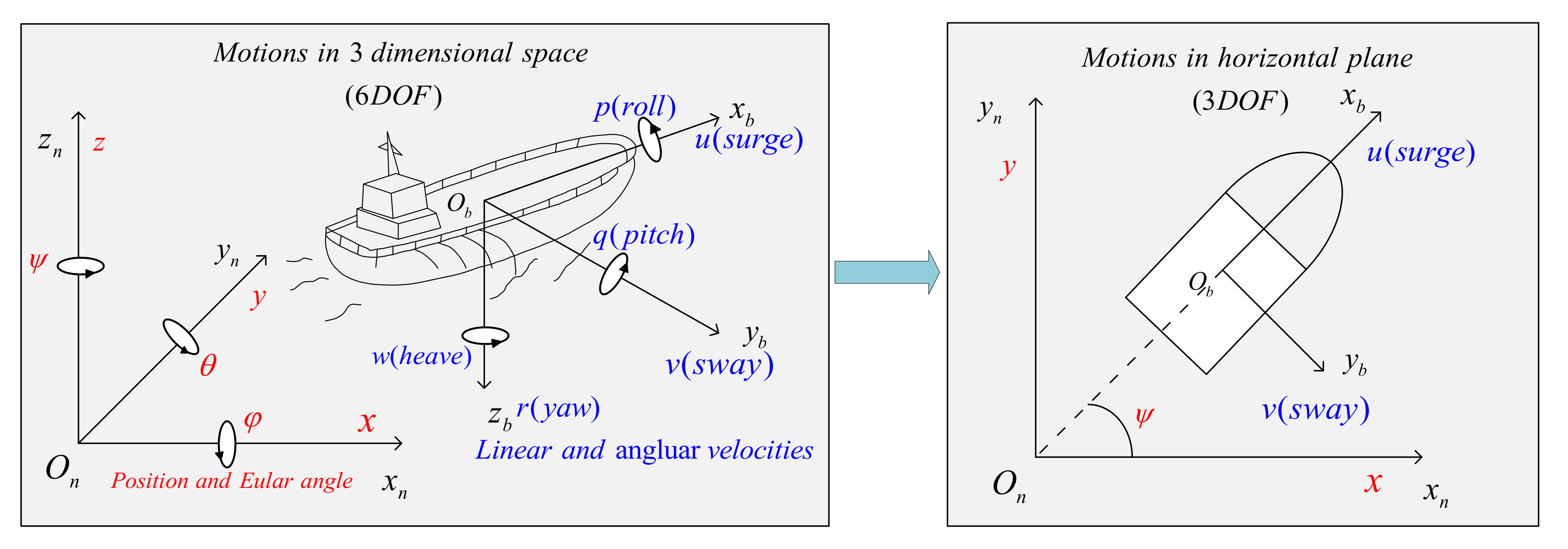
The majority of USVs are typically underactuated and propelled by dual thrusters, with steering being controlled by the differential speed of the dual thrusters. In general, USVs manifest motion along 6 degrees of freedom (DOF). The motions within the horizontal plane are denoted as surge (longitudinal motion), sway (lateral motion), and yaw (rotation about the vertical axis). The remaining three degrees of freedom encompass roll (rotation about the longitudinal axis), pitch (rotation about the transverse axis), and heave (vertical motion), as illustrated in Figure 1.
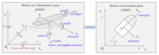
Figure 1.
USV motions in 6 DOF and 3 DOF.
For the control of a USV, the 6 DOF ship model is often simplified into a coupled surge−sway−yaw model, neglecting heave, roll, and pitch motions [33]. Drawing from the content in [34], the state variables and control inputs of the USV control system are typically defined in two coordinate systems: the body-fixed frame and the inertial frame. The body-fixed frame serves as a reference frame fixed to the moving vessel, while the inertial frame can be conceptualized as a global coordinate system, stationary and fixed. The specific definitions are as follows:
where denotes the surge, sway, and yaw rate within the body-fixed coordinate system of the USV; represents the coordinates and attitudes of the USV in the inertial coordinate system, corresponding to the X-axis position, Y-axis position, and yaw angle; and characterizes the three inputs of the USV, corresponding to forward force, lateral force, and steering torque. With reference to the preceding vector model, the kinematic and hydrodynamic models of the USV can be written as follows:
where is the transformation matrix that transforms a variable from the body-fixed coordinate system to the inertial coordinate system; denotes the inertia matrix resulting from the rigid body, while represents the inertia matrix attributed to added mass arising from water resistance; and signifies the Coriolis matrix inherent to USV and is the Coriolis matrix stemming from added mass, both contingent on the operational velocity of the USV. The damping matrix, denoted as D, encompasses both linear and nonlinear damping components. Detailed expressions for these matrices can be found in either Reference [35] or [24].
In accordance with the relationship between the inputs and propellers, the general form of the input vector can be formulated as:
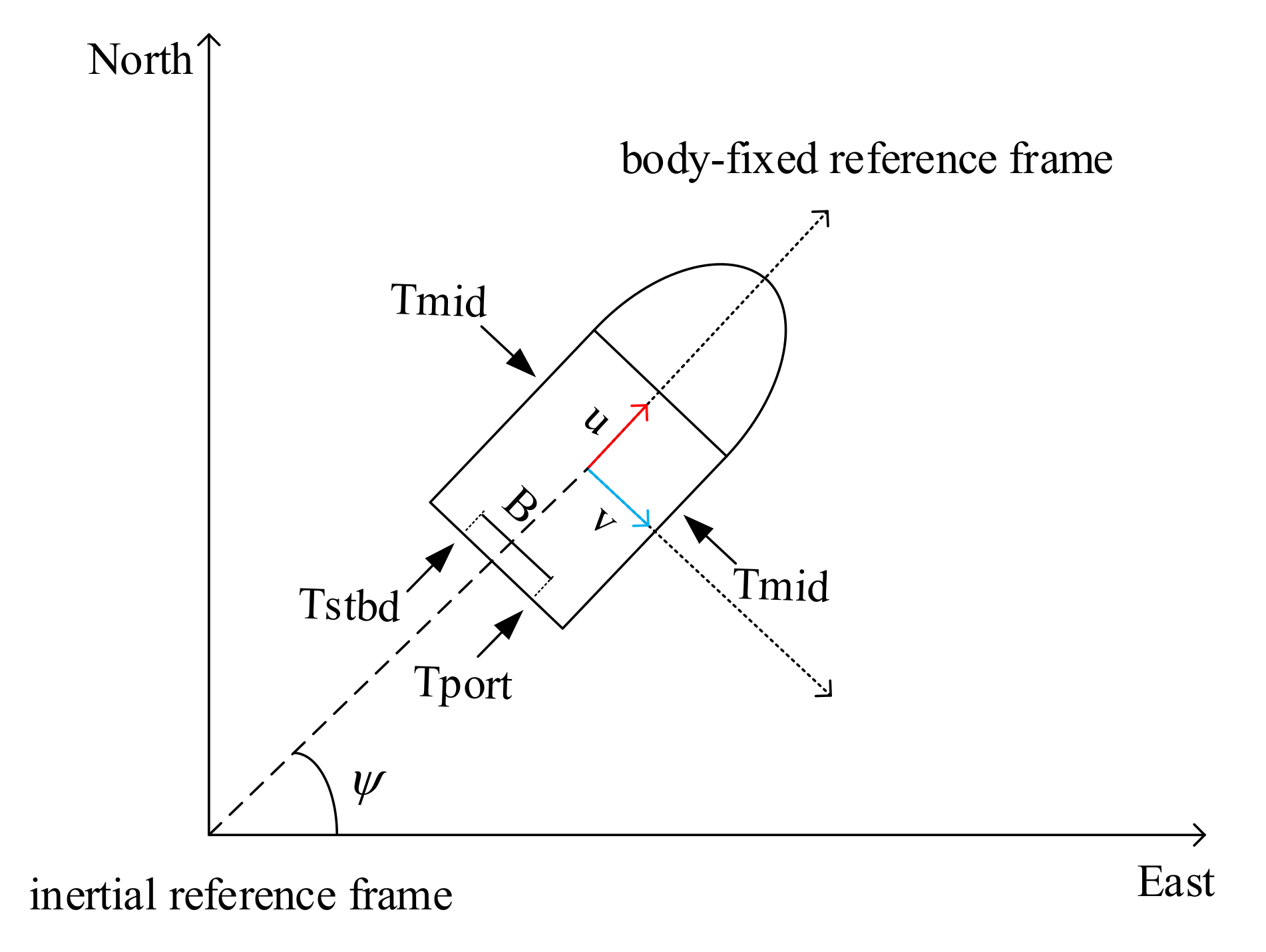
where and represent the magnitudes of forces generated by the rear right and left propellers of the underactuated USV, respectively; B denotes the distance between the two propellers. The lateral thruster generates a force denoted as ; however, this component is absent in underactuated USVs, resulting in . The specific relationship between the thrusters and the USV is visually depicted in Figure 2.
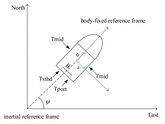
Figure 2.
Force diagram of the USV.
Combining Equations (2) and (3) and selecting the state variable with as the system output, the state space representation of the underactuated USV motion can be expressed as:
Remarkably, the value of for an underactuated USV is set to 0. This arises from the fact that the two propellers at the rear are incapable of independently supplying lateral force for the USV. Consequently, direct control over the sway of the USV is unattainable. Steering torque or interference from external wind and waves may result in sideslip for the USV.
3. Theory and Methodology
MPC originated in the 1970s and was initially applied to the control of chemical processes. MPC primarily comprises three components: model, prediction, and control. The fundamental concept involves predicting future states over several steps and minimizing the disparity with the anticipated future states. This optimization approach is employed to ascertain the optimal control inputs at the present time. Its noteworthy feature is its applicability to multiple-input and multiple-output (MIMO) systems while simultaneously managing multiple constraints. As illustrated in Figure 3, conventional control methods such as PID or backstepping would necessitate designing numerous controllers or control laws based on different control variables of the USV. In contrast, a single MPC controller can address this directly. Given that underactuated USVs inherently involve multiple state variables and constraints, MPC is well-suited for such systems.
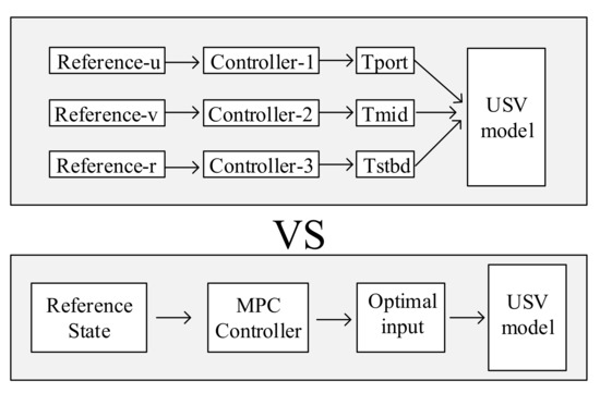
Figure 3.
Advantages of MPC illustration.
The strengths of MPC lie in its ability to handle complex nonlinear systems, multi-objective optimization, and constraints. By predicting future states, MPC provides flexible control strategies and can adaptively adjust to disturbances or changes in the system. As a result, MPC has achieved significant success in various fields such as chemical processes, energy management, robotics, and traffic flow control. However, MPC methods face challenges and limitations, including computational complexity, model errors and uncertainties, and difficulty meeting real-time requirements. The current focuses of researchers are to accelerate solver calculation speed, model identification, and modeling; improve robustness; and expand the application scope of MPC. In conclusion, MPC, as a model-driven optimization control method, has significant practical applications and research value.
MPC methods can be classified into two types: LMPC and NMPC. LMPC involves linearizing the nonlinear model and transforming it into the format of a state-space equation. This process encompasses key steps such as model linearization, discretization, imposing constraints, and formulating the optimization objective function. NMPC, in comparison to LMPC, eliminates the need for model linearization, while the other steps remain similar. For a more comprehensive exploration of the theoretical foundations and derivations of MPC, readers are directed to [36]. The methodology presented in this paper primarily addresses the hydrodynamic model discussed in Section 2, with detailed steps outlined below.
3.1. LMPC
In this subsection, we introduce the specific implementation steps of LMPC, including the linearization and discretization of state space, constraint conditions, and optimization objectives.
3.1.1. Linearization and Discretization of State Space
The essence of LMPC lies in the linearization of the nonlinear model at a specific point. We set the reference state as and the reference input as . Then, performing a first-order Taylor expansion of Equation (5) at the reference point yields the following expression.
Then, the state-space equation can be rewritten as follows:
where, , , and .
Then, it is discretized using the forward Euler method. Its specific expression is .
where , , and . T denotes the sampling period, and represents a 6 × 6 identity matrix.
3.1.2. Constraint Condition
Given the inherent physical limitations of propulsion systems, it becomes necessary to introduce specific constraints on the input. In practical terms, these are transformed into the following representation of inputs:
where represents the predefined control time domain. Within any given control cycle, both the input magnitude ( and ) and the input increment ( and ) of the propeller are subject to boundary constraints.
To more effectively integrate constraints into the control system, a new set of system state variables is introduced here.
Combining Equations (8) and (9) results in a new state-space model expressed as follows:
where , and .
Over the prediction time domains, it is possible to combine all predictive inputs and outputs, leading to the following expression:
where and are the system matrices. is the output sequence over the entire prediction time domain, and denotes the input increment sequence over the entire control time domain. Their specific expressions are as follows:
3.1.3. Optimization Objective
To ensure precise path following and smooth control inputs for USVs, it is essential to formulate an objective function based on the deviation of the system state and the energy consumption of control inputs. Consequently, the objective function for LMPC is defined as follows:
where is L2-norm. Q and R are both weighting matrices, with . In the underactuated state, , while in the fully actuated state, .
After combining Equations (12) and (13) and removing terms unrelated to the control input , the standard quadratic programming (QP) form is as follows:
where , and are column matrices representing the lower and upper bounds of the control input, respectively. The specific composition of matrices
and . ⊗ is Kronecker product.
3.2. NMPC
In contrast to LMPC, NMPC does not require the step of model linearization. It involves discretizing the model, making predictions, and making control decisions based on this discretization. The specific steps include predicting and controlling the state, utilizing the objective function, and employing a nonlinear solver to find the optimal control input. The detailed procedure is outlined below.
3.2.1. Discretization of the State Space
Two commonly utilized methods for discretizing state-space equations are the forward Euler method and the fourth-order Runge–Kutta method. The latter provides higher accuracy in solving differential equations compared with the former but may be slightly slower in terms of computation speed. The forward Euler method has been introduced in Section 3.1.1; here, we present the fourth-order Runge–Kutta method.
For the nonlinear function , given the current state at time k, the solution for the state at time using this method, , can be expressed as follows:
Here, , , , and are intermediate values specifically defined as follows:
where T is the sampling period.
3.2.2. Optimization Objective and Constraints
We designate the prediction horizon of NMPC as and the control horizon as . The task of the nonlinear solver is to find an optimal set of control inputs U that satisfies the predefined minimal objective function. The optimization objective here is slightly different from the objective function in LMPC.
Let k represent the current time, denote the predicted state after i time steps, be the input, and represent the reference state at time i. The optimization objective function is defined as follows:
where is L2-norm, X represents the sequence of state variables across the entire prediction time domain, and U represents the sequence of control inputs throughout the control time domain. The matrix R serves as a smoothing factor for the inputs, aiming to promote a smoother transition between control inputs. and denote the maximum and minimum values, respectively, within the entire input sequence.
3.3. Improved A* Algorithm
The A* algorithm, a classic and widely employed global path planning method, has received considerable attention since its introduction. Researchers have sought to boost its efficiency by implementing measures such as jump point search (JPS) [37] and variable step size search [38]. To achieve smoother paths within the A* algorithm, scholars have explored the use of Bezier curves [39] for trajectory smoothing. In the realm of autonomous driving for unmanned vehicles, the hybrid A* algorithm [40] has been proposed to generate paths that adhere to kinematic constraints. This algorithm takes into account steering angles and velocity to plan smooth paths, proving particularly valuable for tasks like automated parking. Drawing inspiration from the literature in this field, we introduce an improved A* algorithm tailored for USV.
The cost function of the traditional A* algorithm is expressed as
where n is the n-th path point. represents the actual cost from the starting point to the current path point, while represents the heuristic cost from the current point to the endpoint, typically calculated using the Manhattan distance.
The A* algorithm exhibits two primary limitations: first, the planned path tends to be dangerously close to obstacles, and second, the generated path may include straight sections with sudden, sharp angle changes, rendering them unsuitable for direct application in USV. Detailed principles and drawbacks can be found in Reference [41]. In addressing these issues, the following improvement measures are proposed.
- (1)
- To maintain a considerable distance from the edges of obstacles, the obstacle section of the grid map is expanded by N grid cells. The choice of N is dependent on the resolution of the map grid and the size of the USV. As depicted in Figure 4, the black region represents the impassable obstacle area on the map, while the gray region represents an outward extension from the obstacles that, if required, can be traversed. This strategy is implemented to ensure that the path avoids approaching obstacles too closely.
 Figure 4. Obstacle expansion example illustration.
 - (2)
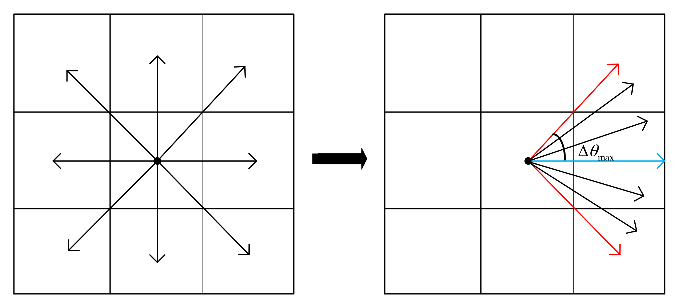
- To ensure the smooth planning of a path, our approach draws inspiration from the hybrid A* algorithm while considering the yaw rate of the USV. Simultaneously, we introduce a fixed step size approach to determine the next path point. Different from the traditional A* algorithm using adjacent grids as the next path point, the proposed approach accelerates the speed of path search.
As illustrated in Figure 5, the left side portrays the original A* search utilizing an 8-neighborhood, whereas the right side shows the modified search area. The blue vector line represents the current yaw angle, and the two red vector lines represent the maximum allowable change in yaw angle between adjacent path points. Discretization takes place within this range, and the black vector lines serve as the search angle, contributing to the creation of a smoother path. The distance between adjacent path points is represented by the parameter .
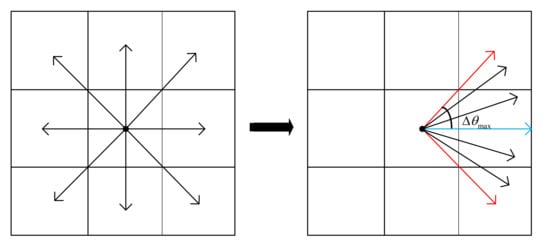
Figure 5.
Enhanced search area conceptual diagram.
In the pursuit of both a smoother path and reduced steering, the improved cost function is formulated as follows:
where denotes the penalty coefficient; represents the angular difference between adjacent path points. We can express as , where and are the yaw angles of the n-th and -th path points, respectively. The range of is , where represents the variable representing the maximum allowable yaw angle difference between neighboring path points. The term is defined as the additional cost incurred when a path point traverses a grid cell. When the cell is white, equals 0. When it is gray, is , and when it is black, is inf.
- (3)
- Generate a path with specified step length intervals and employ third-order B-splines [42] for path optimization. This approach refines the path further to achieve smoothness, enhancing its effectiveness for precise tracking.
4. Simulation Experiment and Analysis
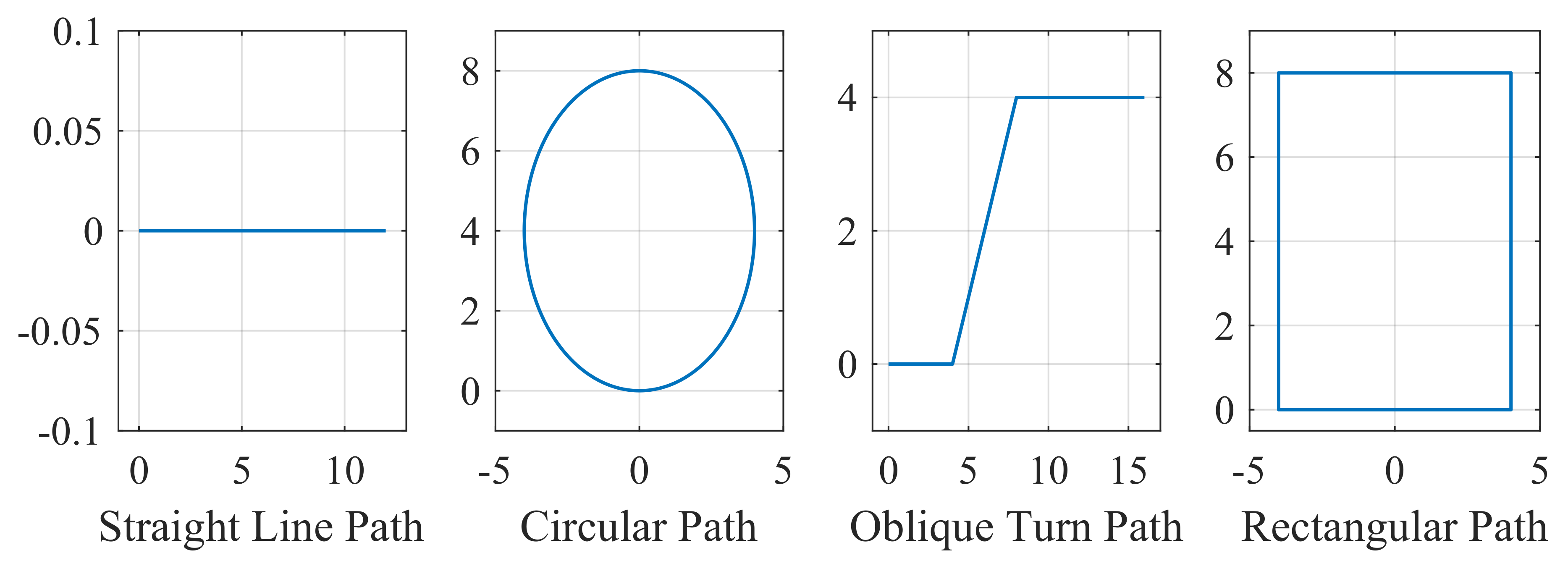
In the MPC simulation, a comprehensive analysis of various articles from the literature and multiple path-following scenarios reveals a significant weakness in the turning capability of underactuated USVs. To tackle this challenge, four sets of simulated paths were designed for underactuated USVs. These include a straight-line path (no turning scenario), a circular path (small-angle turning scenario), an oblique turning path (moderate-angle turning scenario), and a rectangular path (large-angle turning scenario), as depicted in Figure 6.
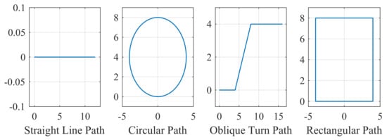
Figure 6.
Four designed paths to track.
The hydrodynamic model data for the simulated USV in this study is obtained from Reference [35]. Table 1 presents detailed parameters related to the USV and hydrodynamics and crucial for Equation (5).

Table 1.
Hydrodynamic parameters.
The definition of reference states in various paths is as follows, where the order of meaning for each variable is defined as .
- (1)
- For the straight-line path, the reference state is defined as .
- (2)
- For the circular path, the reference state is specified as .
- (3)
- For the oblique turning path, the reference state for the straight-line segment remains the same as (1). The reference state for the oblique path segment is defined as .
- (4)
- For the rectangular path, the reference state for the straight-line segment remains unchanged. The right vertical segment is defined as . The remaining horizontal and vertical segments are mostly similar.
In each simulation, the starting time is set at t = 0. T represents the sampling period, which is consistently chosen as 0.1 s. During the simulation process, there exists , where N denotes the number of simulation steps. To evaluate the influence of CPU processors on the MPC solver, all subsequent experiments were carried out on different computers. One utilized an AMD Ryzen 7 5800H CPU (referred to as AMDR7), which is produced by AMD in the United States, considered a standard CPU processor. The other employed a 13th Gen Intel(R) Core(TM) i9-13900KF CPU (referred to as RTM9), which is produced by Intel Corporation in the United States, a higher-end CPU. The simulation based on MATLAB programming language was completed on Matlab R2022a, and the simulation based on C++ programming language was completed on Vscode 1.36 using C++11 standard libraries.
In the following explanations and discussions, unless explicitly specified as a fully actuated USV, the subject is assumed to be an underactuated USV by default.
For subsequent simulation experiments, the default will be to run them on the RTM9 computer, unless specified otherwise for comparative experiments.
4.1. LMPC Simulation
The LMPC is parameterized with the following settings: a prediction horizon of and a control horizon of . The initial states for the USV simulation are specified as . The provided reference inputs are and , with a maximum input limit of and a maximum single-step increment of . The solver employed in this configuration is the classical quadratic programming solver named quadprog.
Upon conducting tests, it was noted that the weight matrices Q and R exhibited variations when tracking each type of path. Despite multiple manual adjustments to these parameters, the tracking performance remained suboptimal. In response, the particle swarm optimization (PSO) algorithm [43] was employed to search for the optimal parameters of the weight matrices. The Q-matrix is utilized to assess the importance of state variables, implying that optimization solutions prioritize certain variables. Simultaneously, the R-matrix constrains the magnitude of input changes. The optimization process in this context concentrates on determining the optimal values for Q.
Given the paper’s emphasis on path following, the evaluation of actual tracking performance depends on specific tracking positions in comparison to the reference path. Consequently, the fitness function for the PSO algorithm is defined as follows:
where is the total number of all path points, and denote the coordinates of the tracking position obtained in the i-th step, and and represent the coordinates of the reference path point. The equation represents the sum of distances between the tracking position and the actual reference position for each step.
4.1.1. Simulation of Underactuated USVs
After extensive simulation, it has been shown that placing a constant Q-matrix may lead to suboptimal tracking performance on paths with varying shapes. Therefore, it is necessary to adjust different parameters according to different paths. Finding the optimal parameters through the PSO algorithm can significantly minimize the impact of parameters on tracking performance. Table 2 presents the optimal weights for the four paths.
Table 2.
Parameters matrices for four paths.
First, let us focus on the straight-line path and the simulation results.
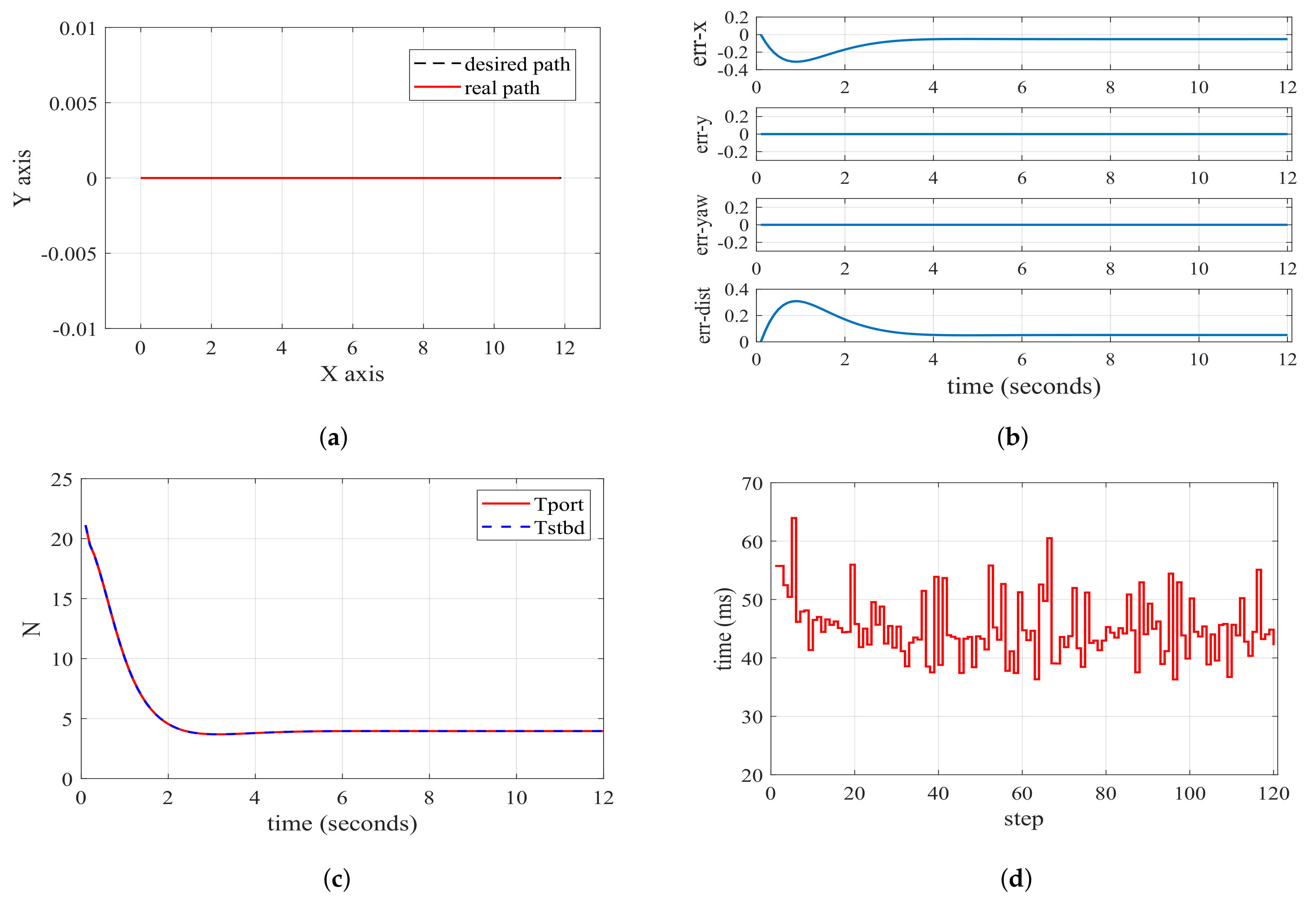
As illustrated in Figure 7b, represents the positional error in the x-direction between the current point and the reference path point. Similarly, denotes the positional error in the y-direction, while is the yaw angle difference. Additionally, corresponds to the Manhattan distance error. In the initial stage, the distance error in the x direction first increases and then decreases toward 0. This phenomenon arises because the initial velocity of the USV is 0, while the reference velocity is 1. Hence, during the initial stage, the actual state of the USV tends to lag behind the reference state. With the thrusters exerting force on the hull, the velocity of the USV gradually increases, eventually aligning with the reference state. It is evident that LMPC achieves fast and accurate tracking of the straight-line path according to Figure 7a. In Figure 7c, both thrusters apply identical forces since the reference path does not require turning and the input changes smoothly. Figure 7d reveals that the solving time is approximately 35 ms per step.
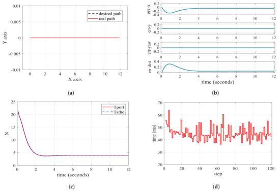
Figure 7.
Diagrams of straight-line path following based on LMPC. (a) path following performance graph; (b) error charts for key performance indicators; (c) actual input for the USV’s Tport and Tstbd; (d) time taken for each step of computation.
Next, we show the simulation results for circular paths. As detailed in Table 2, we have adopted a larger R matrix to minimize input oscillations. This is advantageous when navigating paths with frequent turns, ensuring smoother inputs of thrusters.
Figure 8a,b reveal that the underactuated USV exhibits suboptimal performance in LMPC when navigating circular paths, with a maximum error of approximately 0.3 m. While the basic shape meets requirements, the actual accuracy is relatively low due to position and velocity errors induced by the underactuated USV’s sway during the turning process. The reference position and speed deviate significantly from the current state, particularly concerning the sway, denoted as v. The expected value (reference value) of v is 0, but in practical operation, the underactuated USV’s v is nonzero. The approximate expansion of Equation (6) at the reference point introduces errors, and these errors accumulate as the turning progresses, resulting in unsatisfactory continuous tracking performance. Figure 8c,d represent the two thruster inputs of the USV and the computation time for each round of MPC solver, respectively.
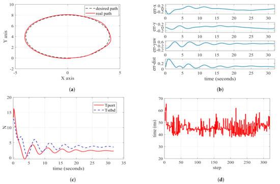
Figure 8.
Diagrams of circular path following based on LMPC. (a) Path following performance graph; (b) error charts for key performance indicators; (c) actual input for USV’s Tport and Tstbd; (d) time taken for each step of computation.
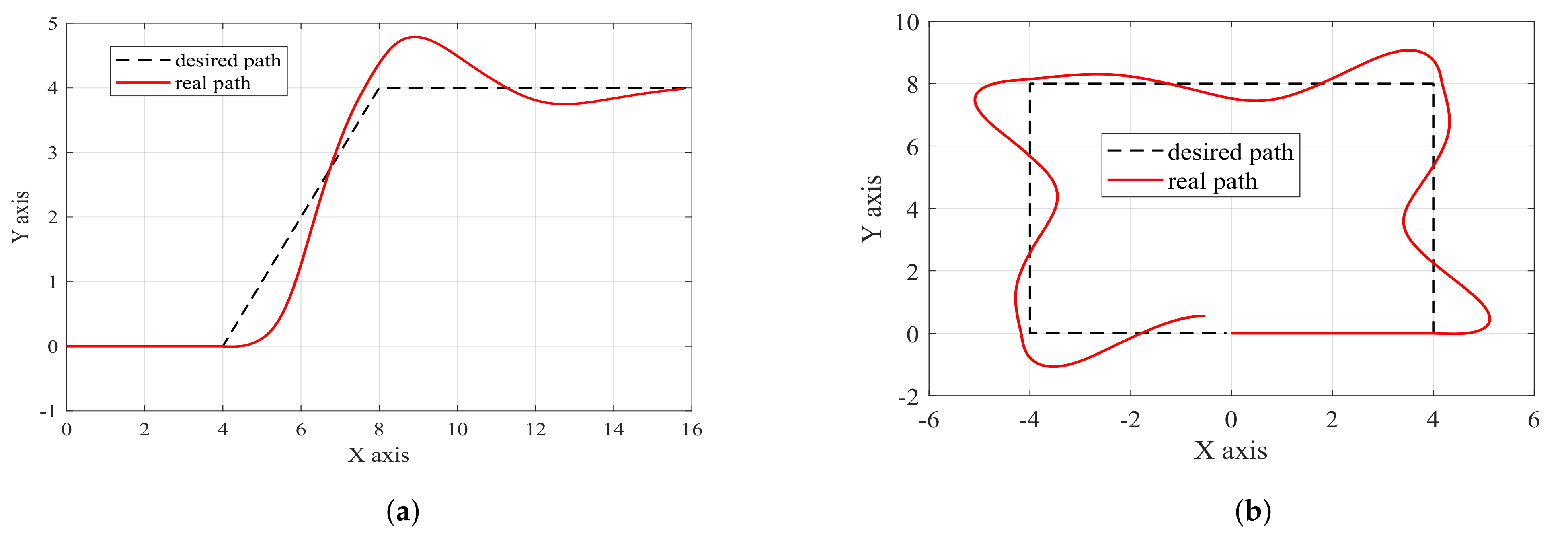
Subsequently, we present the results for the remaining two groups of path following.
From Figure 9, it is apparent that the tracking performances of the oblique turning path and the rectangular path are inferior. The maximum error in the oblique turning path is approximately 1 m in Figure 9a, and the maximum error in the rectangular path is about 1.8 m in Figure 9b. This phenomenon is due mainly to the underactuated USV’s inability to execute instantaneous turns during abrupt and excessive turning angles, resulting in positional and velocity errors. Simultaneously, as the turning angle increases, the disparity between the expected state and the actual state at that moment amplifies. This leads to a larger error when Equation (4) is applied at the reference point, consequently diminishing the effectiveness of steering control for larger angles. To optimize paper space, error diagrams, input diagrams, and computation time diagrams will not be provided.
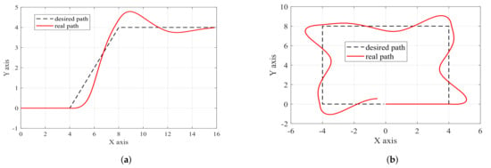
Figure 9.
Path following based on LMPC: two additional paths. (a) Oblique turning path; (b) rectangular path.
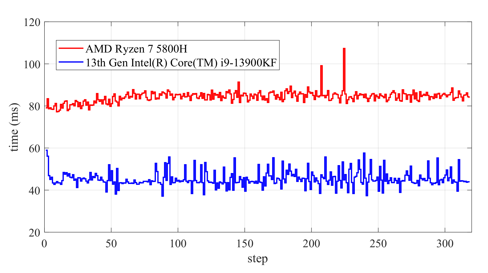
After numerous tests and simulations, it was observed that the time spent in each simulation varies, which is considered a normal occurrence. Figure 10 illustrates the time required to attain a circular path on two different computers. Under RTM9, the average time spent per simulation ranges from approximately 35 to 45 ms, whereas under AMDR7, the average time is approximately 85 to 100 ms, slowing down the solving speed by about twice. It can be seen that the performance of the CPU has a certain impact on the running speed of the program.

Figure 10.
Comparison of time consumption for different CPUs.
In summary, this proves LMPC to be unfit for underactuated USVs for two primary reasons. First, the linearized nonlinear model inherently introduces inaccuracies, and the v of the underactuated USV remains uncontrollable, resulting in a gradual accumulation of errors. As a consequence, the actual control outcomes deviate significantly from the expectations. Second, the optimal weight matrices necessary for different path types vary, and the provided weight matrices Q and R are not universally applicable.
4.1.2. Simulation of Fully Actuated USV
This section is designed to provide stronger support for the earlier viewpoint that LMPC is not fit for controlling underactuated USV. Under the consideration of the infrequent utilization of fully actuated USVs, this section primarily presents simulation results for the path tracking performance of fully actuated USVs based on LMPC, without extensively exploring the topic.
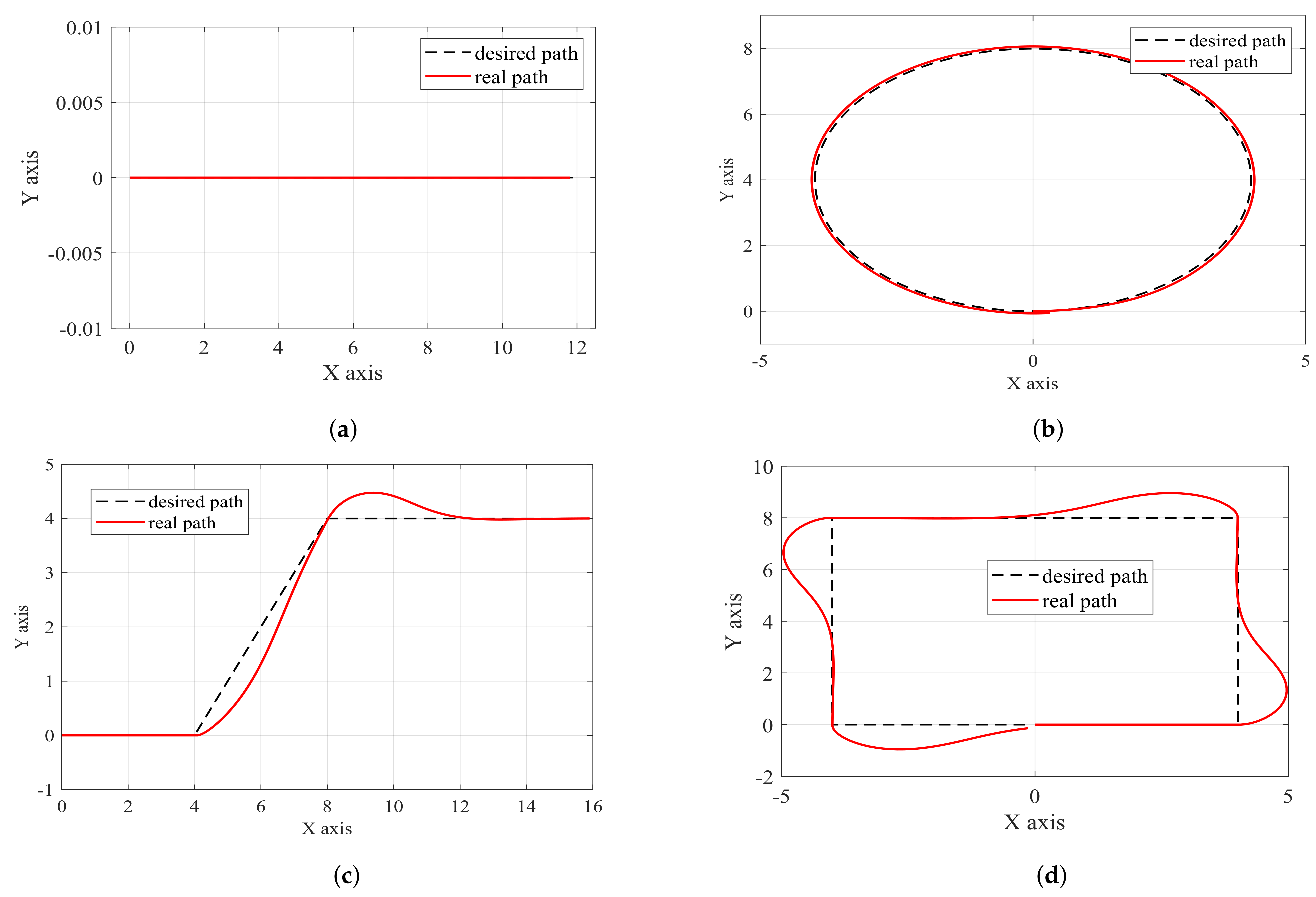
As depicted in Figure 2, a fully actuated USV can generate lateral thrust with a specific input. The uniform use of the basic weight matrix is maintained, with Q = [94, 105, 29, 5, 2, 1] and R = [0.5, 0.5, 0.5]. The other simulation conditions are identical to those in Section 4.1.1, with the addition of an extra control variable. Figure 11 illustrates the specific effect. Figure 11a–d represent the four preset path tracking effect diagrams. The evidence indicates that LMPC exhibits superior control when the USV is fully actuated. While the precision may not reach exceptionally high levels, it represents a significant improvement compared to the underactuated scenario. This observation further supports the idea that LMPC is not fit for the control of underactuated USVs.
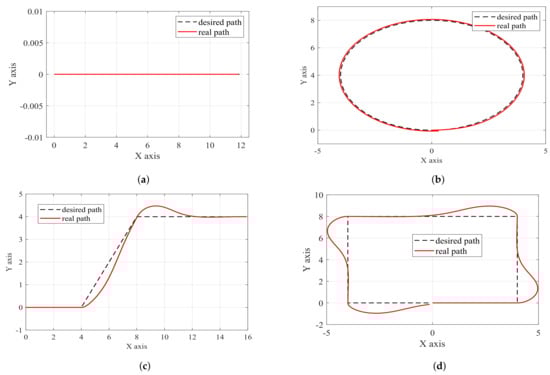
Figure 11.
The path following performance graph of fully actuated USVs. (a) Straight-line path; (b) circular path; (c) oblique turning path; (d) rectangular path.
4.2. NMPC Simulation
Narrowing down our focus to underactuated USVs, it is important to note that NMPC exhibits high precision and can yield effective results for underactuated USVs. Therefore, in our simulations, we exclusively explore scenarios involving underactuated USVs and do not consider fully actuated USVs.
4.2.1. NMPC Based on Fmincon Solver
The fmincon solver serves not only as a nonlinear planner within MATLAB but also as a widely adopted tool among scholars for studying NMPC due to its ability to efficiently address nonlinear programming problems. The simulation parameters include a predicted time domain, = 20, and a controlled time domain, = 19, and NMPC exhibits relatively stable parameter universality. Control weights are set to Q = [30000,30000,1000,0.1,0.1,1000] and R = [0.5,0.5]. The maximum input is 400. The simulation employs the same computer hardware as LMPC.
Given that the straight path is the simplest path, specific simulation results for this case will not be provided here.
In Figure 12, the path following performance of underactuated USVs based on NMPC appears highly satisfactory. Beyond the initial error, subsequent errors gradually converge and diminish, resulting in an overall commendable outcome. In Figure 12b, the specific error representation of Figure 12a illustrates that the tracking error distance stabilizes within 0.1 m. Figure 12c,d represent the two thruster inputs of the USV and the computation time required for each round of the MPC solver, respectively. However, regarding the yaw angle, there is a notable deviation from the expected value. This discrepancy is attributed to the underactuated characteristics of the USV, leading to sideslip. A detailed graphical representation is provided below.
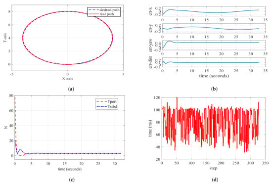
Figure 12.
Diagrams of circular path following based on NMPC. (a) Path following performance graph; (b) error charts for key performance indicators; (c) actual input for USV’s Tport and Tstbd; (d) time taken for each step of computation.
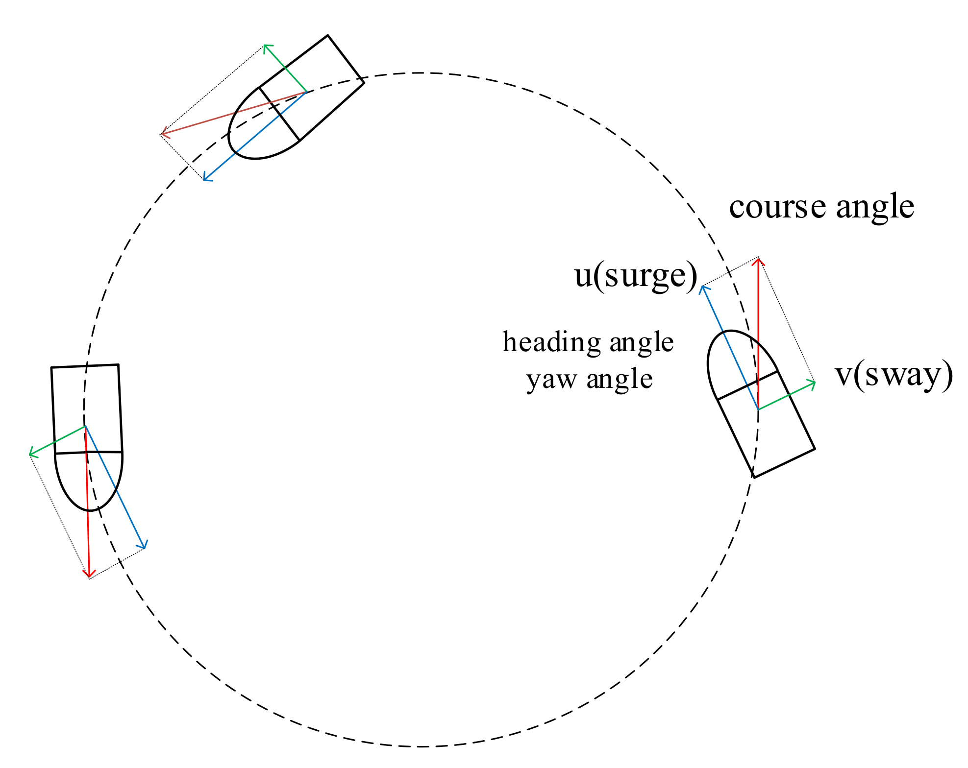
In Figure 13, it is evident that in the body-fixed coordinate system, the yaw angle of the underactuated USV aligns with the velocity u, depicted as a blue vector line in the figure. However, there is a green vector solid line in the velocity v diagram perpendicular to the heading angle, and the sum of these vectors yields the course angle. This aligns with the red vector solid line in the figure, representing the tangent of the circle and the true direction of the USV’s motion. In an ideal state, the USV should not experience sideslip, ensuring that the heading angle, yaw angle, and course angle align. The existence of sideslip velocity v introduces inconsistency between the yaw angle and the true direction of motion. If the USV is fully actuated, then the lateral thruster can eliminate v, allowing only the surge to drive the USV. In such an ideal state, the yaw angle and course angle of the USV coincide. Figure 12c illustrates the input throughout the entire movement, adhering to the predefined maximum range. The solver for each step is time consuming, employing the forward Euler method to solve the differential equation. The average time consumption is approximately 75∼95 ms, indicating a longer processing time compared to LMPC. Here are the path following visualizations for the other two paths.
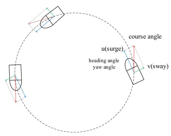
Figure 13.
Motion analysis in the turning process of USV.
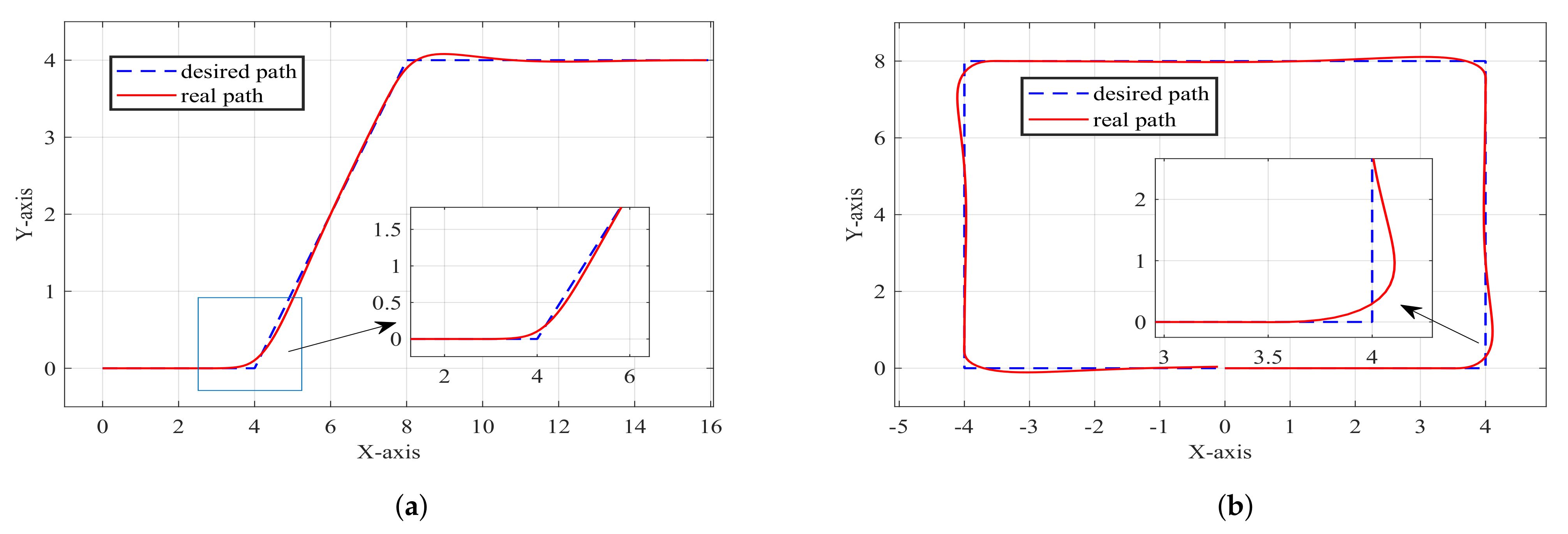
As depicted in Figure 14, NMPC continues to exhibit robust adaptability to underactuated USVs. Figure 14a,b show the tracking effects of oblique and rectangular paths, respectively. Notably, even when confronted with an oblique turning path or a rectangular path, the incurred errors remain minimal. The partially enlarged image provides a closer view, showing the details and the superior tracking performance of NMPC.
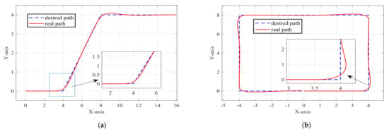
Figure 14.
Path following based on NMPC: two additional paths. (a) Oblique turning path; (b) rectangular path.
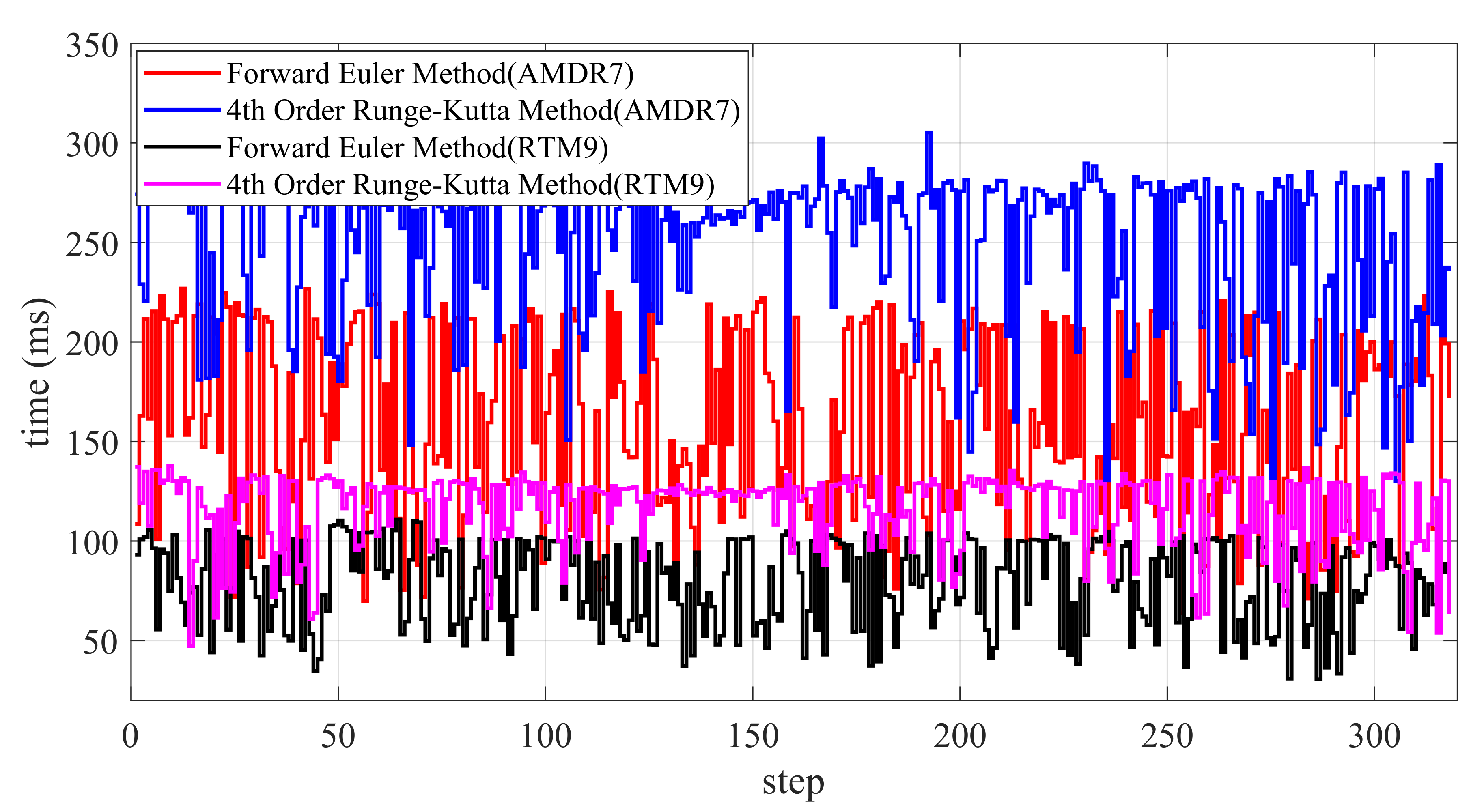
The aforementioned simulation tests were conducted using the RTM9 processor and the forward Euler method. To facilitate a comparative analysis of solution times, the corresponding simulation data for the AMDR7 processor and the fourth-order Runge–Kutta method are presented below. The ultimate path following results across different methods are essentially identical; for brevity, we focus solely on comparing solution times.
Figure 15 presents experimental data obtained from tests conducted on computers equipped with RTM9 and AMDR7 CPUs, respectively. For the RTM9 processor, the average time required for each step using the forward Euler method is 80 ms, while the average time required for the fourth-order Runge–Kutta method is approximately 120 ms. On the contrary, for the AMDR7 processor, the average time for each step using the forward Euler method is 180 ms, while the average time for the fourth-order Runge–Kutta method is approximately 260 ms. Therefore, if precision requirements are not stringent, the forward Euler method proves to be a more favorable choice. Moreover, it is noteworthy that a superior CPU has a certain impact on the realization of real-time NMPC.

Figure 15.
Two different methods and CPUs: computation time comparison ( solver with MATLAB programming language).
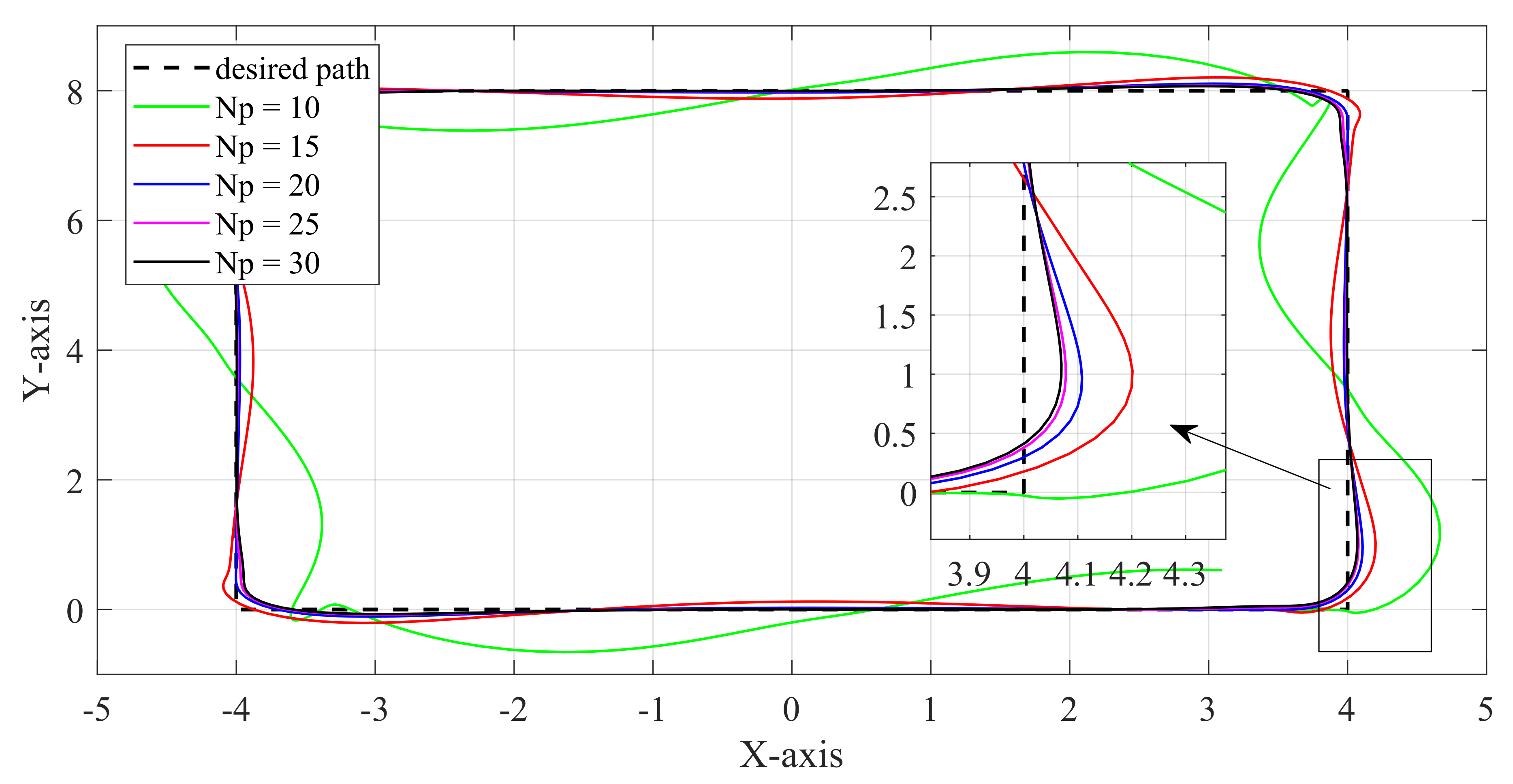
In MPC, the control horizon and the prediction horizon are two parameters that require attention. represents the number of control inputs computed at each time step, but MPC typically uses only the first control input for each step, so has a minimal impact on the control performance. For convenience in programming, is often set to . On the other hand, represents the number of steps forward in the prediction horizon and has a significant impact on the control performance. Specific simulation results for comparison are shown in Figure 16.
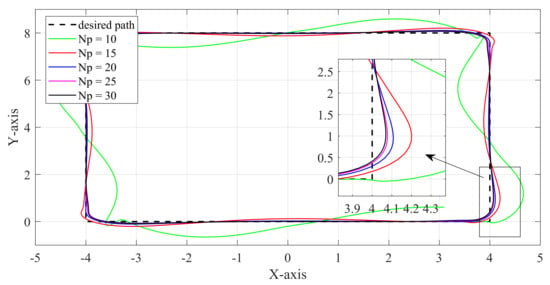
Figure 16.
Tracking results under different parameters .
We designed five sets of comparative experiments for different prediction horizons , with gradually increasing from 10 to 30 with an interval of 5. The results show that the control performance gradually improves as increases. However, when reaches 20, further increasing has diminishing effects on control performance improvement. The average solution time for each step of these 5 experiments is 35 ms, 56 ms, 83 ms, 103 ms, and 113 ms, respectively. It can be observed that as the prediction horizon increases, the computational time required per step also increases. Therefore, finding a balance between control performance and computational efficiency is crucial.
4.2.2. NMPC Based on CasADi Solver
The preceding discussion introduces NMPC based on the fmincon solver, revealing an average solution time of approximately 80 ms per step. This time frame may pose challenges for real-time control applications, where control cycles are typically set at 0.1 s or even shorter, such as 0.05 s or 0.01 s. Although a control cycle of 0.1 s may suffice for non-high-precision control tasks, the time required for the solver to compute the optimal control inputs becomes a crucial factor in determining the adaptability of this algorithm for real-time control. The observed characteristics indicate that the fmincon solver, as described above, may not be well-suited as a real-time solver for NMPC.
Here is an introduction to the CasADi solver [44]. is an open-source software tool designed for general numerical optimization, with a particular emphasis on optimization control, involving differential equations. The performance of this NMPC using the CasADi solver is outstanding, as demonstrated in the following results. With the CasADi solver, the weight matrix is set to Q = [600, 600, 30, 0.1, 0.1, 0.1] and R = [0.05, 0.05]. Next, we focus on its solving efficiency.
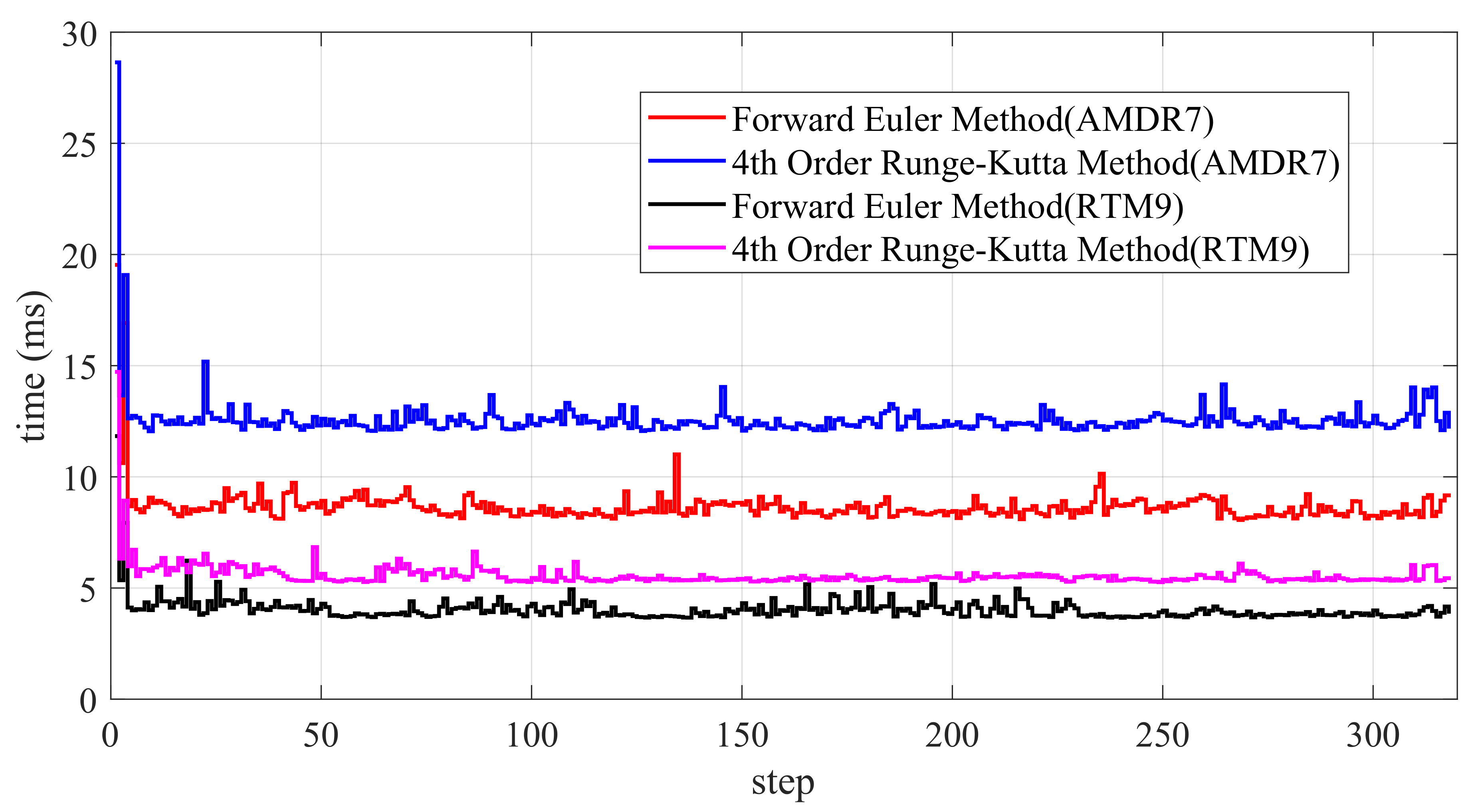
As shown in Figure 17, the CasADi solver surpasses the solver when applied to the same problem. Through extensive testing under the RTM9 CPU, it was observed that the forward Euler method requires approximately 5 ms on average, whereas the fourth-order Runge–Kutta method consumes around 7 ms, resulting in a marginal 2 ms difference. Conversely, under the AMDR7 CPU, the forward Euler method averages about 9 ms, while the fourth-order Runge–Kutta method consumes approximately 13 ms, again exhibiting a 4 ms difference. In comparison to Figure 15, the fmincon solver requires a substantial amount of time to compute the optimal control inputs. On the other hand, the CasADi solver exhibits a shorter and more stable computation time, avoiding significant fluctuations in the solution time.

Figure 17.
Two different methods and CPUs: computation time comparison (CasADi solver with MATLAB programming language).
An interesting observation is that, in the initial stage, the CasADi solver typically exhibits the longest processing time. This phenomenon arises from the fact that, during the initial phase, an arbitrary initial value is assigned to the optimal solution. Consequently, the solver needs to iterate until it reaches the predefined accuracy when solving. Then, we use the values of the optimal control sequence obtained within the preceding control time domains as the initial values for the next solver, thereby accelerating the solver’s computational speed.
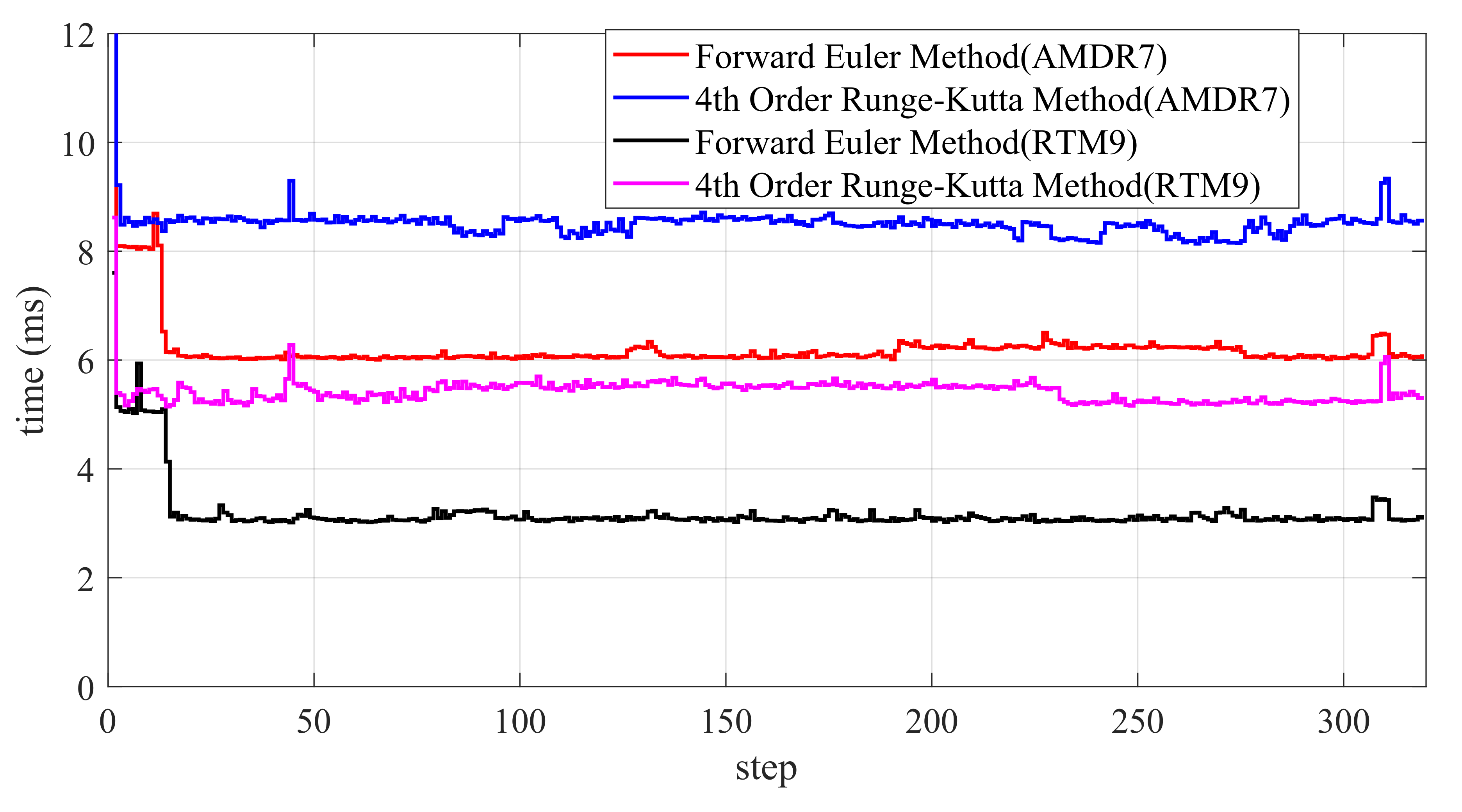
In practical engineering applications, programs recorded in hardware or control programs for host computers are frequently coded using the C++ language, known for its swift execution speed. To align with real-world scenarios, the NMPC algorithm has been implemented in the C++ language, and its runtime performance has been reevaluated. The results are presented in Figure 18.
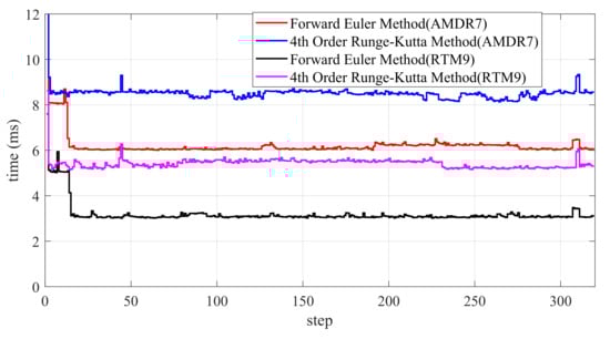
Figure 18.
Two different methods and CPUs: computation time comparison ( solver with C++ programming language).
Figure 18 illustrates that programming in C++ can notably enhance the computational speed of the NMPC solver. Even with a standard AMDR7 processor, both methods can complete the solution within 10 ms. With a high-performance CPU, the solution time using the forward Euler method remains stable at approximately 3 ms, and the more complex fourth-order Runge–Kutta method also stabilizes at 5∼6 ms, demonstrating rapid execution and significant potential for real-time applications.
The following table summarizes the computation time for various methods, CPUs, solvers, and programming languages. The data represent an approximate average derived from multiple tests, as presented in Table 3.
Table 3.
Comparison of computation time across various scenarios: a summary table.
Although our simulation experiments have yielded good results, there are still some potential limitations of NMPC that need to be considered. In particular, there are concerns regarding the computational demands. Our simulations were conducted in a controlled laboratory environment, while the actual operating conditions of USVs are on open water, which may impose certain constraints on the CPU performance and slow down the solution speed. To address this, considering a solving mechanism based on event-triggered approaches may alleviate the computational demands to some extent.
4.3. Actual Path Following Testing Based on NMPC
In Section 3.3, we introduce an improved A* algorithm, and its efficacy will be demonstrated and tested in conjunction with NMPC. The parameters are set as , , and , indicating that the maximum angle difference between adjacent nodes is . The initial and goal positions are set to (8, 8) and (80, 80), respectively, and the initial point’s orientation is set to 0 degrees. After testing, the improved A* algorithm produced 69 path points. The overall count of path points increased to 667 after B-spline optimization.
In the subsequent path following, the calculation approach for the reference state is outlined below.
where represents the reference state of the k-th path point and . Both and are derived from the path points optimized by B-spline.
In Figure 19, the original A* algorithm produces a path that closely adheres to the obstacle, resulting in a steep turn that is impractical for the robot to track. Conversely, the path generated by the improved A* algorithm overcomes these limitations, as denoted by the blue dashed line, presenting a smoothly turning path that adheres to specified turning constraints. The path further undergoes B-spline smoothing, depicted by the dashed red line, which essentially aligns with the blue dashed line, indicating that the unsmoothed path also exhibits good feasibility. The locally enlarged image along the path demonstrates that B-spline smoothing provides additional compensation for occasional lack of smoothness in specific locations.
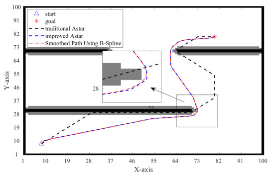
Figure 19.
Original and improved paths of the A* algorithm.
Analyzing Figure 20a, it is evident that the USV controlled by NMPC achieves commendable following performance on the planned path. Simultaneously, examination of the velocity curve presented in Figure 20b reveals that the USV stabilizes at approximately 2 m/s during the intermediate stage. As the USV approaches the goal position, its velocity u gradually decreases. Figure 20c illustrates the input signals, indicating relatively smooth inputs that adhere to the defined constraints. Figure 20d illustrates the solver’s solving time throughout the simulation process, revealing that each round of solving consistently remains below 10 ms. This demonstrates a notably fast computational performance.
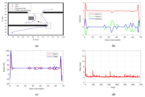
Figure 20.
Diagrams of path following generated by improved A* based on NMPC. (a) Path following performance graph; (b) path following velocity graph; (c) actual input for USV’s Tport and Tstbd; (d) time taken for each step of computation.
5. Conclusions and Discussion
In this paper, the theory and simulation experiments of LMPC and NMPC were thoroughly analyzed and discussed. The following conclusions are drawn from the study.
- (1)
- In the context of underactuated USV control, we conducted a detailed comparative analysis of various paths in this paper. The findings clarify the reasons why LMPC is unfit for underactuated USV control and suggest that NMPC is the better choice.
- (2)
- In addressing real-time concerns, this paper extensively discussed the performance of NMPC under varying solvers, CPUs, and programming languages. Utilizing the CasADi solver with C++ as the programming language, the paper showed that even with a standard CPU, NMPC achieved a solution speed within 10 ms. In conclusion, the study affirms the potential of NMPC for real-time control applications.
- (3)
- For the universality of NMPC, we conducted simulations across a range of paths to support this perspective. Ultimately, the improved A* algorithm was employed to generate paths for testing, demonstrating its efficacy in achieving robust path following.
The path tracking based on NMPC and path planning based on the improved A* algorithm proposed in this study have important practical significance and application value. First, the path tracking method based on NMPC can assist USVs in accurately following predefined paths during mission execution. By performing online optimization of control inputs, the USV can dynamically adjust its heading and speed in order to stay on the desired path and reduce deviations. This is particularly important for applications that require high-precision positioning and navigation, such as ocean mapping and the detection of waterborne targets. Second, the path planning method based on the improved A* algorithm can help USVs find optimal paths in complex environments. By considering obstacles, environmental constraints, and mission objectives, the A* algorithm can generate a safe and efficient path that enables the USV to navigate successfully. This is especially useful for applications that involve operating in congested or hazardous areas, such as harbor patrols and maritime rescues.
In the future, it is hoped that NMPC can become a popular control algorithm for underactuated USVs. However, NMPC relies on the precise mathematical model of an underactuated USV. Therefore, modeling an underactuated USV is an important research work.
Author Contributions
Conceptualization, W.L.; methodology, W.L.; software, W.L.; validation, W.L.; formal analysis, W.L. and X.Z.; investigation, W.L.; data curation, Y.W.; writing—original draft preparation, W.L.; writing—review and editing, X.Z.; visualization, Y.W. and S.X.; supervision, Y.W. and S.X.; project administration, X.Z.; funding acquisition, X.Z. All authors have read and agreed to the published version of the manuscript.
Funding
This work was supported by a project from the National Natural Science Foundation of China under grant number 62073210.
Institutional Review Board Statement
Not applicable.
Informed Consent Statement
Not applicable.
Data Availability Statement
Data is contained within the article.
Conflicts of Interest
Author Songbo Xie was employed by the company Shandong Laigang Yongfeng Steel Corporation. The remaining authors declare that the research was conducted in the absence of any commercial or financial relationships that could be construed as a potential conflict of interest.
References
- Xie, J.; Zhou, R.; Luo, J.; Peng, Y.; Liu, Y.; Xie, S.; Pu, H. Hybrid partition-based patrolling scheme for maritime area patrol with multiple cooperative unmanned surface vehicles. J. Mar. Sci. Eng. 2020, 8, 936. [Google Scholar] [CrossRef]
- Liu, Z.; Zhang, Y.; Yu, X.; Yuan, C. Unmanned surface vehicles: An overview of developments and challenges. Annu. Rev. Control. 2016, 41, 71–93. [Google Scholar] [CrossRef]
- Zhao, Y.; Qi, X.; Ma, Y.; Li, Z.; Malekian, R.; Sotelo, M.A. Path following optimization for an underactuated USV using smoothly-convergent deep reinforcement learning. IEEE Trans. Intell. Transp. Syst. 2020, 22, 6208–6220. [Google Scholar] [CrossRef]
- Woo, J.; Yu, C.; Kim, N. Deep reinforcement learning-based controller for path following of an unmanned surface vehicle. Ocean Eng. 2019, 183, 155–166. [Google Scholar] [CrossRef]
- Karnani, C.; Raza, S.A.; Asif, M.; Ilyas, M. Adaptive Control Algorithm for Trajectory Tracking of Underactuated Unmanned Surface Vehicle (UUSV). J. Robot. 2023, 2023, 4820479. [Google Scholar] [CrossRef]
- Huang, Z.; Liu, X.; Wen, J.; Zhang, G.; Liu, Y. Adaptive navigating control based on the parallel action-network ADHDP method for unmanned surface vessel. Adv. Mater. Sci. Eng. 2019, 2019, 7697143. [Google Scholar] [CrossRef]
- Liao, Y.; Jiang, Q.; Du, T.; Jiang, W. Redefined output model-free adaptive control method and unmanned surface vehicle heading control. IEEE J. Ocean. Eng. 2019, 45, 714–723. [Google Scholar] [CrossRef]
- Wang, R.; Li, D.; Miao, K. Optimized radial basis function neural network based intelligent control algorithm of unmanned surface vehicles. J. Mar. Sci. Eng. 2020, 8, 210. [Google Scholar] [CrossRef]
- Liu, H.; Lin, J.; Yu, G.; Yuan, J. Robust adaptive self-Structuring neural network bounded target tracking control of underactuated surface vessels. Comput. Intell. Neurosci. 2021, 2021, 2010493. [Google Scholar] [CrossRef]
- Elhaki, O.; Shojaei, K. Robust saturated dynamic surface controller design for underactuated fast surface vessels including actuator dynamics. Ocean Eng. 2021, 229, 108987. [Google Scholar] [CrossRef]
- Liu, Z.; Zhang, Y.; Yuan, C.; Luo, J. Adaptive path following control of unmanned surface vehicles considering environmental disturbances and system constraints. IEEE Trans. Syst. Man Cybern. Syst. 2018, 51, 339–353. [Google Scholar] [CrossRef]
- Peng, Z.; Liu, E.; Pan, C.; Wang, H.; Wang, D.; Liu, L. Model-based deep reinforcement learning for data-driven motion control of an under-actuated unmanned surface vehicle: Path following and trajectory tracking. J. Frankl. Inst. 2023, 360, 4399–4426. [Google Scholar] [CrossRef]
- Qu, X.; Jiang, Y.; Zhang, R.; Long, F. A Deep Reinforcement Learning-Based Path-Following Control Scheme for an Uncertain Under-Actuated Autonomous Marine Vehicle. J. Mar. Sci. Eng. 2023, 11, 1762. [Google Scholar] [CrossRef]
- Wang, J.; Wu, Z.; Yan, S.; Tan, M.; Yu, J. Real-time path planning and following of a gliding robotic dolphin within a hierarchical framework. IEEE Trans. Veh. Technol. 2021, 70, 3243–3255. [Google Scholar] [CrossRef]
- Cao, H.; Xu, R.; Zhao, S.; Li, M.; Song, X.; Dai, H. Robust trajectory tracking for fully-input-bounded actuated unmanned surface vessel with stochastic disturbances: An approach by the homogeneous nonlinear extended state observer and dynamic surface control. Ocean Eng. 2022, 243, 110113. [Google Scholar] [CrossRef]
- Yan, Y.; Yu, S.; Gao, X.; Wu, D.; Li, T. Continuous and Periodic Event-Triggered Sliding-Mode Control for Path Following of Underactuated Surface Vehicles. IEEE Trans. Cybern. 2023, 54, 449–461. [Google Scholar] [CrossRef]
- Zhou, W.; Fu, J.; Yan, H.; Du, X.; Wang, Y.; Zhou, H. Event-triggered approximate optimal path-following control for unmanned surface vehicles with state constraints. IEEE Trans. Neural Netw. Learn. Syst. 2021, 34, 104–118. [Google Scholar] [CrossRef]
- Liang, H.; Li, H.; Xu, D. Nonlinear model predictive trajectory tracking control of underactuated marine vehicles: Theory and experiment. IEEE Trans. Ind. Electron. 2020, 68, 4238–4248. [Google Scholar] [CrossRef]
- Fossen, T.I.; Pettersen, K.Y.; Galeazzi, R. Line-of-sight path following for dubins paths with adaptive sideslip compensation of drift forces. IEEE Trans. Control. Syst. Technol. 2014, 23, 820–827. [Google Scholar] [CrossRef]
- Song, L.; Xu, C.; Hao, L.; Yao, J.; Guo, R. Research on PID Parameter Tuning and Optimization Based on SAC-Auto for USV Path Following. J. Mar. Sci. Eng. 2022, 10, 1847. [Google Scholar] [CrossRef]
- Liu, L.; Wang, D.; Peng, Z. ESO-based line-of-sight guidance law for path following of underactuated marine surface vehicles with exact sideslip compensation. IEEE J. Ocean. Eng. 2016, 42, 477–487. [Google Scholar] [CrossRef]
- Taghavifar, H.; Qin, Y.; Hu, C. Adaptive immersion and invariance induced optimal robust control of unmanned surface vessels with structured/unstructured uncertainties. Ocean Eng. 2021, 239, 109792. [Google Scholar] [CrossRef]
- Liu, C.; Li, C.; Li, W. Computationally efficient MPC for path following of underactuated marine vessels using projection neural network. Neural Comput. Appl. 2020, 32, 7455–7464. [Google Scholar] [CrossRef]
- Han, S.; Wang, L.; Wang, Y. A potential field-based trajectory planning and tracking approach for automatic berthing and COLREGs-compliant collision avoidance. Ocean Eng. 2022, 266, 112877. [Google Scholar] [CrossRef]
- Zhou, X.; Wu, Y.; Huang, J. MPC-based path tracking control method for USV. In Proceedings of the 2020 Chinese Automation Congress (CAC), IEEE, Shanghai, China, 6–8 November 2020; pp. 1669–1673. [Google Scholar]
- Dong, Z.; Zhang, Z.; Qi, S.; Zhang, H.; Li, J.; Liu, Y. Autonomous Cooperative Formation Control of Underactuated USVs based on Improved MPC in complex ocean environment. Ocean Eng. 2023, 270, 113633. [Google Scholar] [CrossRef]
- Wang, L.; Chu, X.; Liu, C. Different drive models of USV under the wind and waves disturbances MPC trajectory tracking simulation research. In Proceedings of the 2015 International Conference on Transportation Information and Safety (ICTIS), IEEE, Wuhan, China, 25–28 June 2015; pp. 563–568. [Google Scholar]
- Liu, C.; Hu, Q.; Wang, X.; Yin, J. Event-triggered-based nonlinear model predictive control for trajectory tracking of underactuated ship with multi-obstacle avoidance. Ocean Eng. 2022, 253, 111278. [Google Scholar] [CrossRef]
- Huang, T.; Chen, Z.; Gao, W.; Xue, Z.; Liu, Y. A USV-UAV Cooperative Trajectory Planning Algorithm with Hull Dynamic Constraints. Sensors 2023, 23, 1845. [Google Scholar] [CrossRef] [PubMed]
- Abdelaal, M.; Fränzle, M.; Hahn, A. NMPC-based trajectory tracking and collison avoidance of underactuated vessels with elliptical ship domain. IFAC 2016, 49, 22–27. [Google Scholar]
- Zheng, X.; Wang, J.; Zhang, S.; Zhang, C. Nonlinear Model Predictive Path Following for an Unmanned Surface Vehicle. In Proceedings of the Global Oceans 2020: Singapore–US Gulf Coast, IEEE, Biloxi, MS, USA, 5–30 October 2020; pp. 1–5. [Google Scholar]
- Batkovic, I.; Gupta, A.; Zanon, M.; Falcone, P. Experimental Validation of Safe MPC for Autonomous Driving in Uncertain Environments. arXiv 2023, arXiv:2305.03312. [Google Scholar] [CrossRef]
- Fossen, T.I. Handbook of Marine craft Hydrodynamics and Motion Control; John Wiley & Sons: Hoboken, NJ, USA, 2011. [Google Scholar]
- Fossen, T.I. Marine Control Systems—Guidance, Navigation, and Control of Ships, Rigs and Underwater Vehicles; Marine Cybernetics; Springer: Trondheim, Norway, 2002; ISBN 82 92356 00 2. [Google Scholar]
- Skjetne, R.; Smogeli, Ø.N.; Fossen, T.I. A nonlinear ship manoeuvering model: Identification and adaptive control with experiments for a model ship. MIC J. 2004, 25, 3–27. [Google Scholar] [CrossRef]
- Rawlings, J.; Mayne, D. Postface to model predictive control: Theory and design. Nob. Hill Pub. 2012, 5, 155–158. [Google Scholar]
- Zheng, T.; Xu, Y.; Zheng, D. AGV path planning based on improved A-star algorithm. In Proceedings of the 2019 IEEE 3rd Advanced Information Management, Communicates, Electronic and Automation Control Conference (IMCEC), IEEE, Chongqing, China, 11–13 October 2019; pp. 1534–1538. [Google Scholar]
- Erke, S.; Bin, D.; Yiming, N.; Qi, Z.; Liang, X.; Dawei, Z. An improved A-Star based path planning algorithm for autonomous land vehicles. Int. J. Adv. Robot. Syst. 2020, 17, 1729881420962263. [Google Scholar] [CrossRef]
- Hong-han, Z.; Liming, G.; Tao, C.; Lu, W.; Xun, Z. Global path planning methods of UUV in coastal environment. In Proceedings of the 2016 IEEE International Conference on Mechatronics and Automation, IEEE, Harbin, China, 7–10 August 2016; pp. 1018–1023. [Google Scholar]
- Dolgov, D.; Thrun, S.; Montemerlo, M.; Diebel, J. Practical search techniques in path planning for autonomous driving. Ann. Arbor. 2008, 1001, 18–80. [Google Scholar]
- Pan, H.; Guo, C.; Wang, Z. Research for path planning based on improved astart algorithm. In Proceedings of the 2017 4th International Conference on Information, Cybernetics and Computational Social Systems (ICCSS), IEEE, Dalian, China, 24–26 July 2017; pp. 225–230. [Google Scholar]
- Tang, G.; Tang, C.; Claramunt, C.; Hu, X.; Zhou, P. Geometric A-star algorithm: An improved A-star algorithm for AGV path planning in a port environment. IEEE Access 2021, 9, 59196–59210. [Google Scholar] [CrossRef]
- Bian, L.; Che, X.; Chengyang, L.; Jiageng, D.; Hui, H. Parameter optimization of unmanned surface vessel propulsion motor based on BAS-PSO. Int. J. Adv. Robot. Syst. 2022, 19, 17298814211040688. [Google Scholar] [CrossRef]
- Mehrez, M.W.; Mann, G.K.; Gosine, R.G. Stabilizing NMPC of wheeled mobile robots using open-source real-time software. In Proceedings of the 2013 16th International Conference on Advanced Robotics (ICAR), IEEE, Montevideo, Uruguay, 25–29 November 2013; pp. 1–6. [Google Scholar]


Disclaimer/Publisher’s Note: The statements, opinions and data contained in all publications are solely those of the individual author(s) and contributor(s) and not of MDPI and/or the editor(s). MDPI and/or the editor(s) disclaim responsibility for any injury to people or property resulting from any ideas, methods, instructions or products referred to in the content. |
© 2024 by the authors. Licensee MDPI, Basel, Switzerland. This article is an open access article distributed under the terms and conditions of the Creative Commons Attribution (CC BY) license (https://creativecommons.org/licenses/by/4.0/).