Abstract
The marine environment of the Arctic Ocean has changed rapidly in recent decades. We used reanalysis data and observational data to explore the variations in the upper ocean heat content (OHC) of the Canadian Basin (CB) and the variations in the temperature profiles of the Southern Canadian Basin (SCB). Both the reanalysis data and observational data show increasing trends for the OHC of the CB from 1993 to 2023. Compared to the World Ocean Atlas data (WOA 18/23), the reanalysis data (ORAS5 or GLORYS12V1) significantly underestimated the values of the upper OHC of the Canadian Basin. To explain the OHC differences, the Ice-Tethered Profiler (ITP) observational data were used to analyze the variations in the vertical temperature profiles. We found that the reanalysis data remarkably underestimated the maximum temperatures of the subsurface Pacific warm water and its increasing trend. Based on the short-term prediction results from the Bi-LSTM neural network, we forecasted that the upper OHC will continue to increase in the SCB, mainly due to the warming of the intermediate Atlantic warm water. The research results provide a valuable reference for assessing and improving climate-coupled models.
1. Introduction
The Arctic Ocean is an important component of the Earth’s climate system and is experiencing significant changes in response to global warming. Many studies have pointed out that the loss of Arctic sea ice is largely attributed to atmospheric forcing [1,2]. However, with the intensification of the Atlantic warm water flow into the Arctic [3], the release of ocean heat reduces the formation of sea ice in the winter, and the loss rate is comparable to the losses caused by atmospheric heat forcing [4]. This has been termed the ‘Atlantification’ phenomenon that has occurred in the Eurasian Basin, including the Nansen and Amundsen Basins [4]. It is clear that the heat content of the upper ocean plays an important role in the melting and thawing of sea ice. Far from the above regions, in the Canadian Basin (CB), the freezing time of multi-year sea ice is three months later at the bottom than at the surface, and sea ice starts to melt more than half a month earlier at the bottom than at the surface [5]. Therefore, we aimed to determine whether the upper heat content in the CB is also affected by the changes in the North Atlantic warm water.
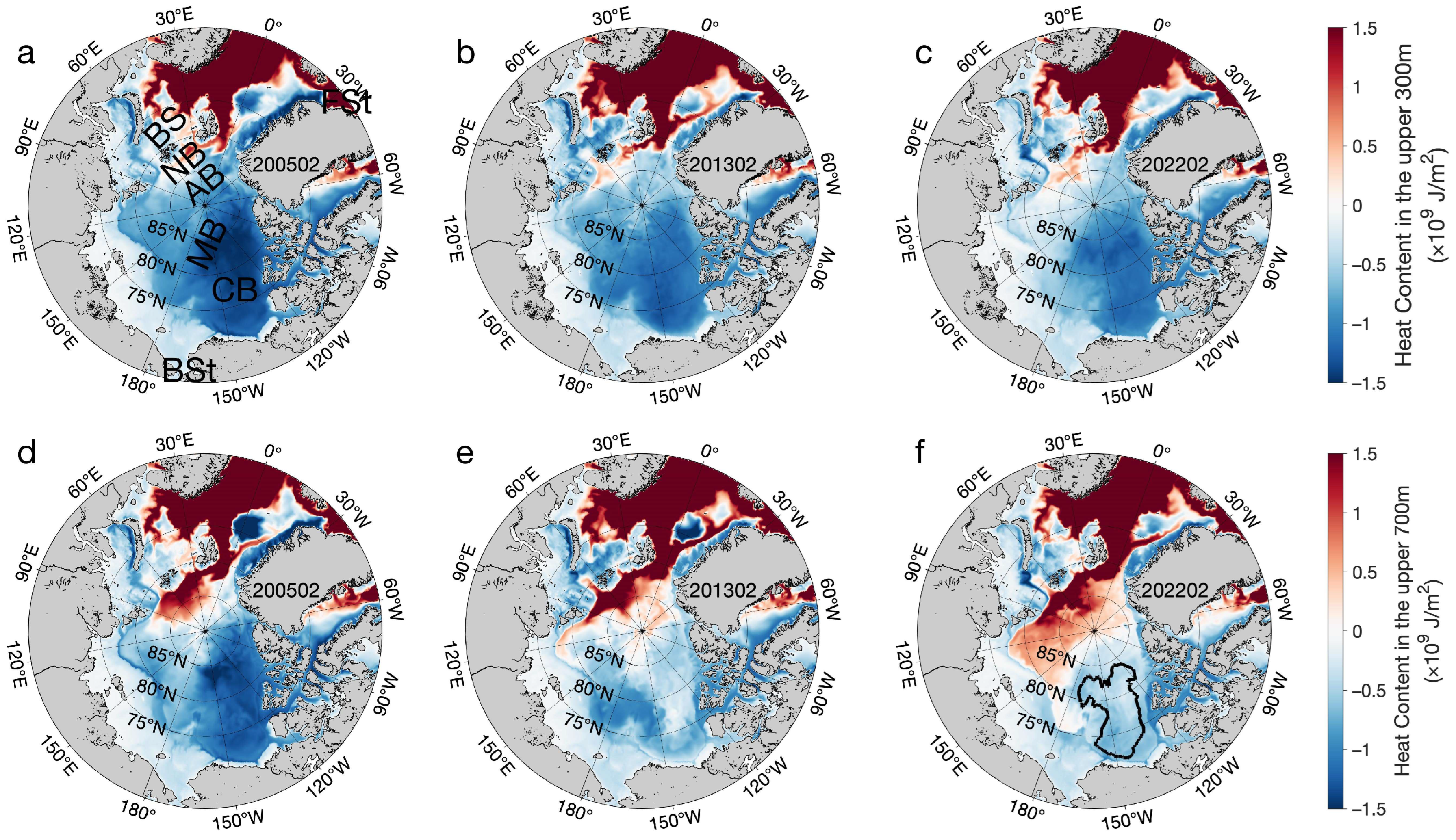
There is a wind-driven and anticyclonic flow field called the Beaufort Gyre around the Canadian Basin. It is one of the Arctic Ocean’s primary circulations and a major freshwater reservoir [6]. The water bodies in the Canadian Basin are complex. The main sources of the upper and middle water masses are the shelf runoff, Arctic Pacific water masses, and mid-Atlantic water in the CB [7]. From top to bottom, the water mass can be divided into surface low-salinity mixed water, subsurface warm water, winter mixed residual water, Pacific summer water, Pacific winter water, and North Atlantic warm water [8]. On the other hand, Arctic sea ice area reaches its maximum in February during the winter and its minimum in September during the summer. Correspondingly, the OHC in the uppermost layer has obvious seasonal variations with minimum values in February and maximum values in September. To eliminate the effect of seasonal fluctuations, we chose the representative February OHC to analyze its overall trend variations. Based on the reanalysis data from ORAS5 (described below), the spatial distribution of the oceanic heat content (OHC) is shown in Figure 1. Compared to the OHC in February of 2005, 2013, and 2022, the OHC in the upper 300 and 700 m increased significantly throughout the upper Arctic Ocean. In the CB, far from the Fram Strait and the Barents Sea, which are the Atlantic inflow entrances, variations in the upper 300 m OHC (300 m OHC) and the upper 700 m OHC (700 m OHC) increase significantly, while the variation in the OHC originating in the Pacific Ocean is not significant. Thus, we wondered whether the increased OHC in the upper layers of the CB is caused by the enhanced Atlantic warm water.
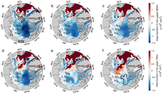
Figure 1.
The ocean heat content in the upper 300 m (a–c) and upper 700 m (d–f) in February of 2005, 2013, and 2022. The data are from ORAS5. The Fram Strait (FSt), Bering Strait (BSt), Barents Sea (BS), Canadian Basin (CB), Nansen Basin (NB), Amundsen Basin (AB), and Makarov Basin (MB) are indicated in (a). In (f), the 3000 m depth isobath in the CB is marked by a black line.
To answer this question, we used open access data, including reanalysis data (ORAS5 and GLORYS12V1) and observational data (WOA and ITPs), to study the variations in the OHC and the vertical temperature profiles in the CB. The remainder of this paper is structured as follows: Section 2 and Section 3 describe the data and methods used, Section 4 outlines the results, and Section 5 presents the conclusions and discussion.
2. Data
2.1. Ice-Tethered Profiler Data
The Ice-Tethered Profiler (ITP) data are available on the following website: http://www.whoi.edu/itp (accessed on 27 January 2024). These data include time, position (longitude and latitude), pressure, temperature, and salinity. Some profiles contain other information, e.g., oxygen, chlorophyll, and velocity components. The open access ITP data are available on three levels. Level 1 includes the raw data. The Level 2 real-time data are averaged in 2 db bins. Salinity is derived from the bin-averaged pressure, temperature, and conductivity. Level 3 data products are derived for each ITP system after its mission has been completed. It is the corrected final data, gridded to a resolution of 1 m.
As of January 2024, a total of 141 ITPs has been deployed. More than 1000 vertical temperature and salinity profiles have been collected from the Arctic Ocean. These profiler data cover the period from 24 August 2004 to 27 January 2024. The spatio-temporal distribution of the trajectories of these ITPs can be seen in Figure 2. The data are mainly concentrated in the Central and Southern CB regions. The number distribution of the ITP profiles in the Canadian Basin and a histogram of the monthly ITP profile numbers in the Southern Canadian Basin (black box) are shown in Figure 3.
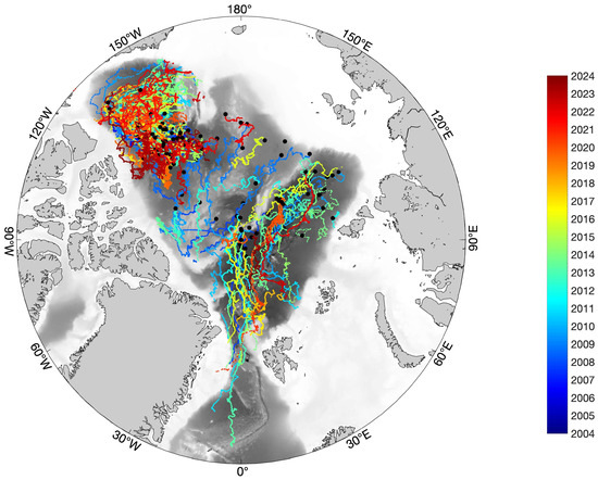
Figure 2.
The spatio-temporal distribution of the ITP trajectories. The solid black dots represent the deployment locations. The color represents the drift date.
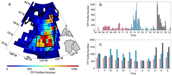
Figure 3.
The number distribution of the ITP profiles in the Canadian Basin from August 2004 to January 2024. (a) The number of ITP profiles within 1° × 1° bins. The black dots indicate the region of bins with ITP profile numbers greater than 500. (b) A histogram of the monthly ITP profile numbers within the southern sector of the Canadian Basin (bounded by thick black lines). (c) A histogram of the monthly ITP profile numbers from August 2004 to December 2012 (pink), from January 2013 to December 2018 (blue), and from January 2019 to December 2023 (gray).
We used Level 3 data and then Level 2 data. We used a total of 125 ITPs, with 114 ITPs on Level 3 and 11 ITPs on Level 2 (Table 1). The number of ITPs without data records is shown in gray. We uniformly averaged these available data (temperature and salinity) every 2 m from the surface, starting from 1 m to a depth of 700 m.

Table 1.
The available Ice-Tethered Profiler data and the variables.
2.2. Ocean Reanalysis Data
Ocean Reanalysis System 5 (ORAS5) combines model data with observations. It provides monthly mean data from global ocean and sea ice reanalysis, including ocean heat content variables for the upper 300 and 700 m. The heat content was calculated by integrating the temperature, seawater density, and specific heat capacity from the surface to depths of 300 and 700 m. Monthly data from 1958 to the present can be downloaded from the Copernicus Climate Data Store at https://cds.climate.copernicus.eu (accessed on 18 January 2024).
2.3. Word Ocean Atlas
The World Ocean Atlas (WOA) is a collection of objectively analyzed and quality-controlled temperature, salinity, and other data based on profile data from the World Ocean Database (WOD). It can be used to verify numerical simulations of the ocean. WOA18 contains the decadal average temperature for the 1995–2004 and 2005–2017 periods. WOA23 contains the ocean temperature over the 1991–2020 period at selected standard depths. The temperature data are shown as monthly values on the 1° grid and as seasonal values on the 1/4° grid. The WOA can be downloaded at https://www.ncei.noaa.gov/products/world-ocean-atlas (accessed on 27 January 2024).
2.4. GLORYS12V1 Data
GLORYS12V1 is a global eddy-resolving physical ocean and sea ice reanalysis tool with a 1/12° horizontal resolution and 50 standard vertical levels, and it is also distributed by CMEMS. It covers the altimetry period from 1993 to the present. GLORYS12V1 assimilates altimeter sea level anomalies, satellite sea surface temperatures, sea ice concentrations, and in situ vertical temperature and salinity profiles. Quality assessments have shown that GLORYS12V1 effectively captures the expected interannual climate variability signals for ocean and sea ice. More details on GLORYS12V1 can be found in the study by Jean-Michel et al. [9]. GLORYS12V1 datasets are available through the Copernicus Marine Environment Monitoring Service (CMEMS; https://marine.copernicus.eu/; accessed on 27 January 2024).
3. Methods
3.1. Ocean Heat Content
OHC is used to quantify the rate of global warming. A high OHC can disrupt marine ecosystems, bleach coral, contribute to extreme weather events such as hurricanes, and affect sea level rise [10]. The ocean heat content anomaly (OHCA) is a comparison of the current OHC with long-term averages. The OHC describes the amount of heat stored in the upper layers of the ocean, as shown in Equation (1):
where is the specific heat capacity, is the density of the seawater, is the temperature of the seawater, and is the freezing temperature. To ensure simplicity and consistency with the heat content from ORAS5, we set . The heat content was obtained using Equation (2):
where or .
Note that the temperature of seawater in the polar region is often below zero. Using zero as the reference temperature results in a negative heat content for seawater. Since this study does not focus on the heat release and absorption involved in the melting and freezing processes of sea ice, but rather on the variation trend in the heat content, we set . For other cases, it is recommended to use the freezing point of seawater to calculate the heat content.
3.2. Bi-Directional LSTM
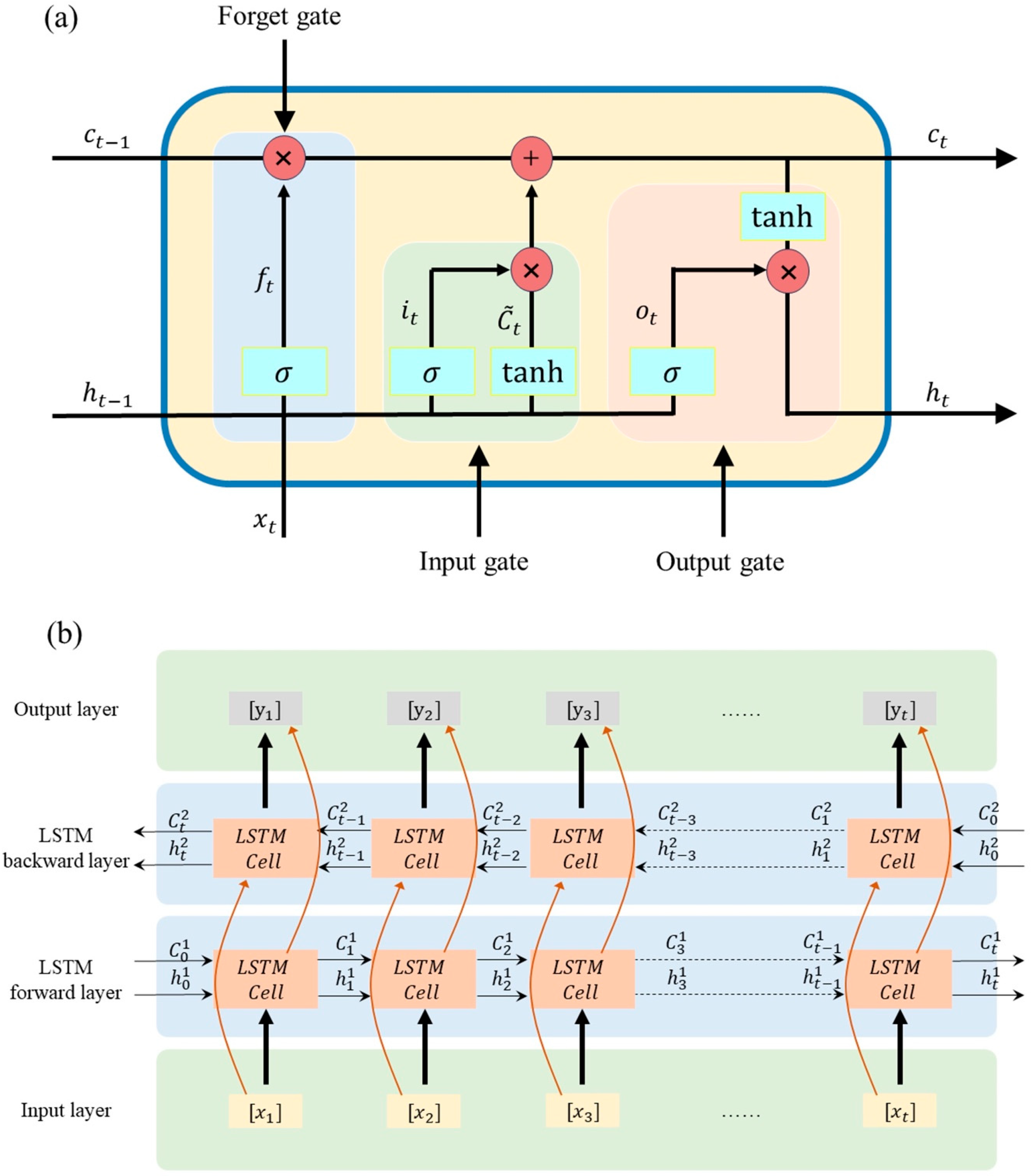
The long short-term memory (LSTM) neural network is a variant of the recurrent neural network (RNN) proposed by Hochreiter and Schmidhuber in 1997 for long time series [11]. Unlike a traditional RNN, the LSTM can effectively solve the gradient vanishing problem in the process of training long time series. The LSTM cell mainly consists of an input gate, a forgetting gate, and an output gate, and the information in the current cell is processed by these three gates to selectively “remember” or “forget” some data points (Figure 4a). The LSTM network and its multiple variants have already demonstrated their ability to accurately predict the sea surface temperature and chlorophyll-a concentrations [12,13], and they have been successfully used for wave prediction [14].
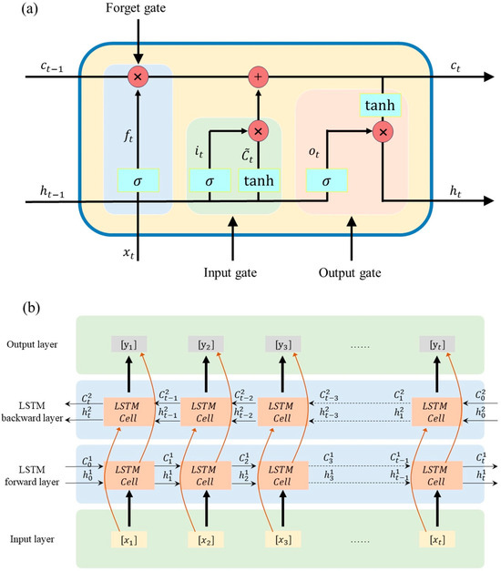
Figure 4.
(a) An internal structure diagram of a long short-term memory (LSTM) cell. (b) The framework of a Bi-LSTM (bi-directional LSTM) prediction network.
Bi-directional LSTM (BiLSTM) contains LSTM cells in two directions: one from the beginning to the end of the sequence (forward direction), and the other from the end to the beginning (reverse direction). This allows the network to capture both past and future information within the sequence data, thereby enhancing the model’s ability to model complex dependencies within the sequence (Figure 4b). The Bi-LSTM can improve the understanding of time series data and make accurate predictions. Jiang et al. [15] successfully used Bi-LSTM and BOA-Argo data to predict and analyze ocean temperature and salinity profiles.
Bi-LSTM has the advantages of using long time series data for training and having a bidirectional structure, allowing it to process both backward and forward sequential data and keep past and future information. Therefore, we chose Bi-LSTM to predict the temperature profile in our study.
Due to the limited frequency of data sampling in this study, we were constrained to using monthly ORAS5 and GLORYS12V1 data for model training and monthly mean ITP data for prediction. Monthly data from ORAS5 and GLORYS12V1 covering the 1993 to 2022 period were used to generate the corresponding training and validation datasets. The data volume ratio of the training dataset to the validation dataset was 4:1. Monthly data from 2022 to 2023 were used as a testing dataset to examine the performance. Due to discontinuities in the ITP observational data, we only used yearly data from 2021 for the testing set to make predictions for the temperature profile. It is possible to improve the model’s predictive performance in the future when high temporal resolution data become available.
4. Results
4.1. The Heat Content in the Upper Canadian Basin Ocean
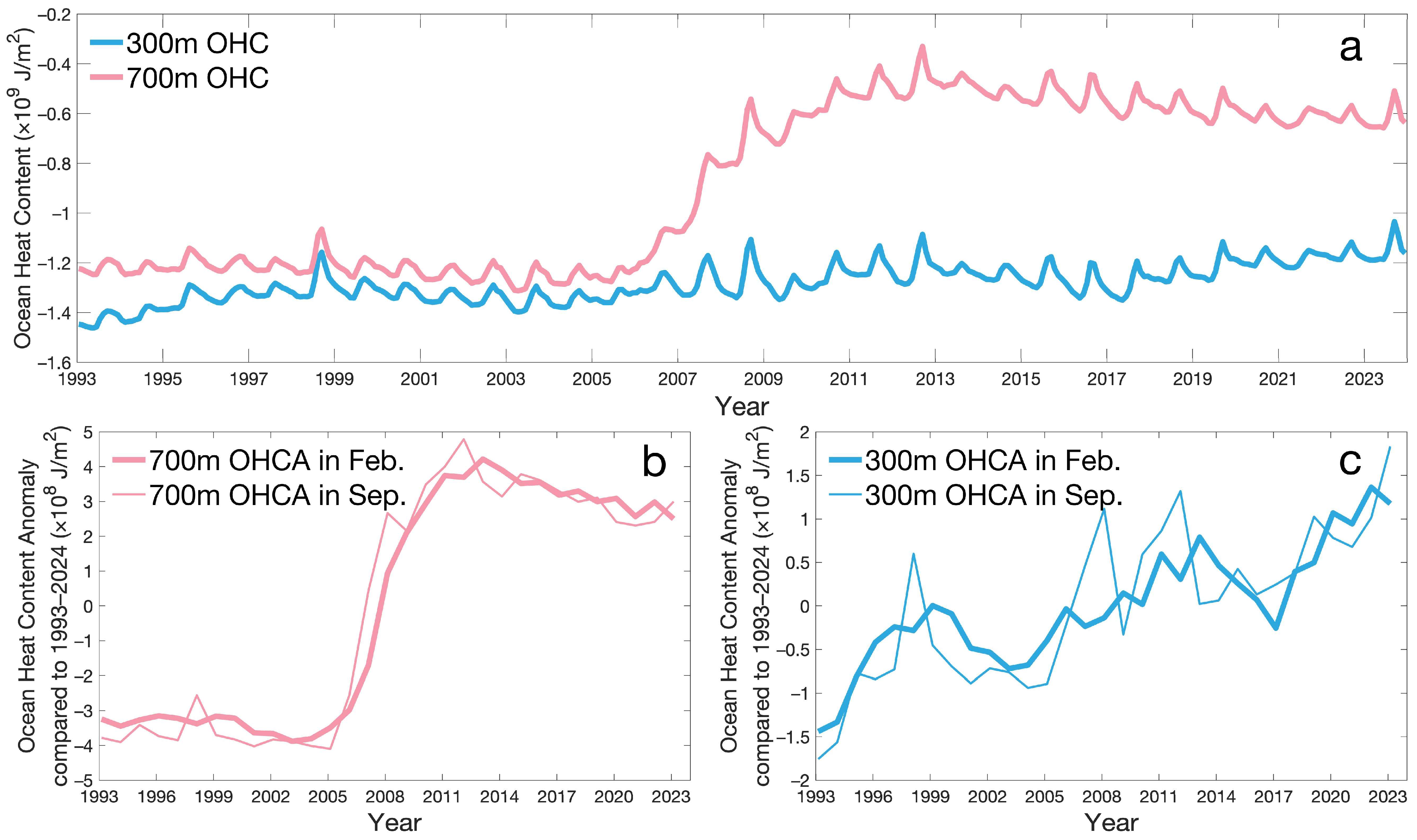
As seen from the ORAS5 data, the spatial distribution of the OHC shows that Atlantic warm water has influenced the Barents Sea and the Nansen Basin in the Pan-Arctic Ocean (Figure 1). When comparing the OHC in February of 2005, 2013, and 2022, it can be seen that the invasion of Atlantic warm water through the Fram Strait has intensified over time. The OHC significantly increased in the Makorov Basin and the CB, which is far away from the Fram Strait. When comparing the 300 m OHC and the 700 m OHC, the changes in the 700 m OHC were more obvious in the CB. The time series of the average 300 m OHC and 700 m OHC over the CB (bounded by the black 3000-isobath line in Figure 1) is shown in Figure 5. There were fluctuating seasonal variations and a rapid change from 2005 to 2013 (Figure 5a). To avoid the seasonal fluctuating effects of the surface OHC, we chose typical months, February and September, to analyze the variations in the upper 300 m OHC anomaly (300 m OHCA) and upper 700 m OHC anomaly (700 m OHCA). The changes in the 700 m OHC were about from 1993 to 2023. The February and September 700 m OHCAs had rapid changes between 2005 and 2013 but had slightly decreasing changes since 2014 (Figure 5b), while the February and September 300 m OHCAs continuously increased from 1993 to 2023. The change in the 300 m OHCA was about from 1993 to 2023 (Figure 5c). As seen in Figure 1, the abrupt increase in the 700 m OHC could be explained by the intensified intermediate Atlantic water in the CB. The variation in the 300 m OHC was continuous and different from that in the 700 m OHC.
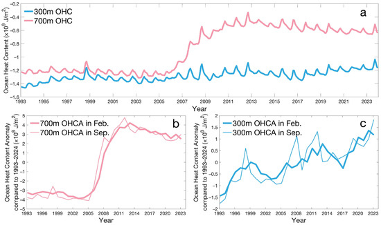
Figure 5.
(a) The variations in the ocean heat content for the upper 300 and 700 m in the Canadian Basin. (b) The variations in the February and September OHCAs for the upper 700 m. (c) The variations in the February and September OHCAs for the upper 300 m.
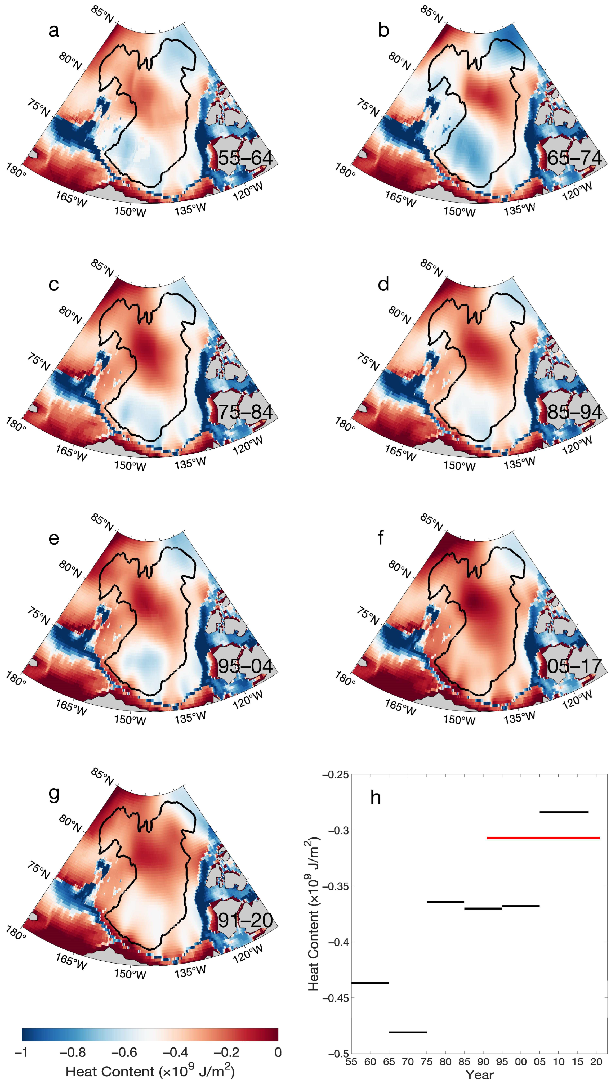
To confirm the above ORAS5 reanalysis results, we used the observational data sets, WOA18 and WOA23, to validate the spatio-temporal variations in the OHC in the CB. WOA18 provides decadal data from 1955 to 2017, and WOA23 provides climatological data covering the period from 1991 to 2020. The spatial 700 m OHC derived using WOA18 from the 1955–1964, 1965–1974, 1975–1984, 1985–1994, 1995–2004, and 2005–2017 periods is shown in Figure 6a–f, and WOA23 data from the 1991–2020 period are shown in Figure 6g. There were two discrepant 700 m OHC cores in the CB. One was located in the Northern CB, and the other was in the Southern CB. They were also located in the region of Beaufort Gyre, which is a wind-driven and anticyclonic flow field across the CB [6]. Although they clearly had different values, the overall spatial 700 m OHC underwent obvious increasing variations (Figure 6a–f). Since we were limited by the observational data, we only had the phased variations in the average 700 m OHC within the CB (Figure 6h). The range of the mean 700 m OHC value in the CB was between and from 1955 to 2020 (Figure 6h). The spatial and temporal variations in the 700 m OHC appeared to grow stepwise. For WOA18, the mean 700 m OHC value in the CB was slightly lower than from 1995 to 2004 (Figure 6h), while for ORAS5, it was about from 1993 to 2006 (Figure 5a). For WOA23, the mean 700 m OHC value in the CB was about from 2005 to 2017 (Figure 6h), while for ORAS5, it was about starting from 2013 (Figure 5a). Although the reanalysis results show the same increasing trend as the observational results, the reanalysis OHC (ORAS5) values were lower than the observational OHC (WOA18/23) values. To explain the OHC differences, it is necessary to analyze the variations in the vertical temperature profiles.
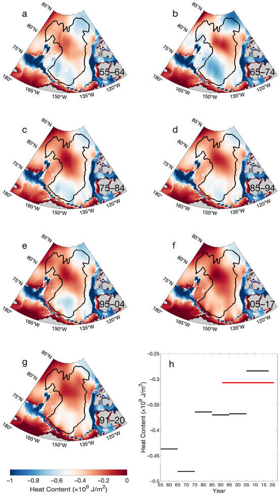
Figure 6.
The spatial plots of the climatological upper 700 m OHC derived using WOA18 from the (a) 1955–1964, (b) 1965–1974, (c) 1975–1984, (d) 1985–1994, (e) 1995–2004, and (f) 2005–2017 periods and using WOA23 from the (g) 1991–2020 period. (h) The phase variations in the average OHC within the CB bounded by the 3000 m isobath lines. The segmented black lines are the spatially averaged OHC values derived from WOA18 (1955–2017), and the thick red line is derived from WOA23 (1991–2020).
4.2. Changes in Temperature Profiles in the Southern Canadian Basin
There was a marked cold core in the 700 m OHC spatial distributions over the Southern CB (Figure 6a–g). It underwent a distinct transition from a cold spot to a warm spot. We also considered the volume of the observational ITP data concentrated in this region (Figure 3). Therefore, we focused on the analysis of the vertical temperature profiles in the Southern Canadian Basin (SCB). Except for the data from ORAS5 and WOA, we additionally used the available observations (ITP) and other reanalysis data (GLORYS12V1) to analyze the vertical temperature profiles.
The quantity distribution of the ITP profiles within the 1° × 1° bins in the CB are shown in Figure 3a. The bins with more than 500 profiles are indicated by the black dots. The ITP data were relatively uniformly concentrated in the southern sector bounded by the thick black lines in the CB. Thus, there were enough data available in the SCB to analyze the changes in the vertical temperature. According to the monthly distribution of ITP profile volumes (Figure 3b), we divided the data into three periods, namely from January 2004 to December 2012, from January 2013 to December 2018, and from January 2004 to March 2023. The data volume from 2014 to 2015 and from 2020 to 2021 were relatively abundant. These three phases had comparable amounts of monthly data and were suitable for climatological comparison (Figure 3c).
The spatio-temporal average temperature profiles derived from the ITP data are shown in Figure 7a. There were two maximum values in every vertical profile. The first one stood for subsurface Pacific warm water (SPWW), and the second one stood for intermediate Atlantic warm water (IAWW). The heat content in the upper ocean was influenced by IAWW and SPWW. The IAWW was warmer than the SPWW and had a larger water body than the SPWW.

Figure 7.
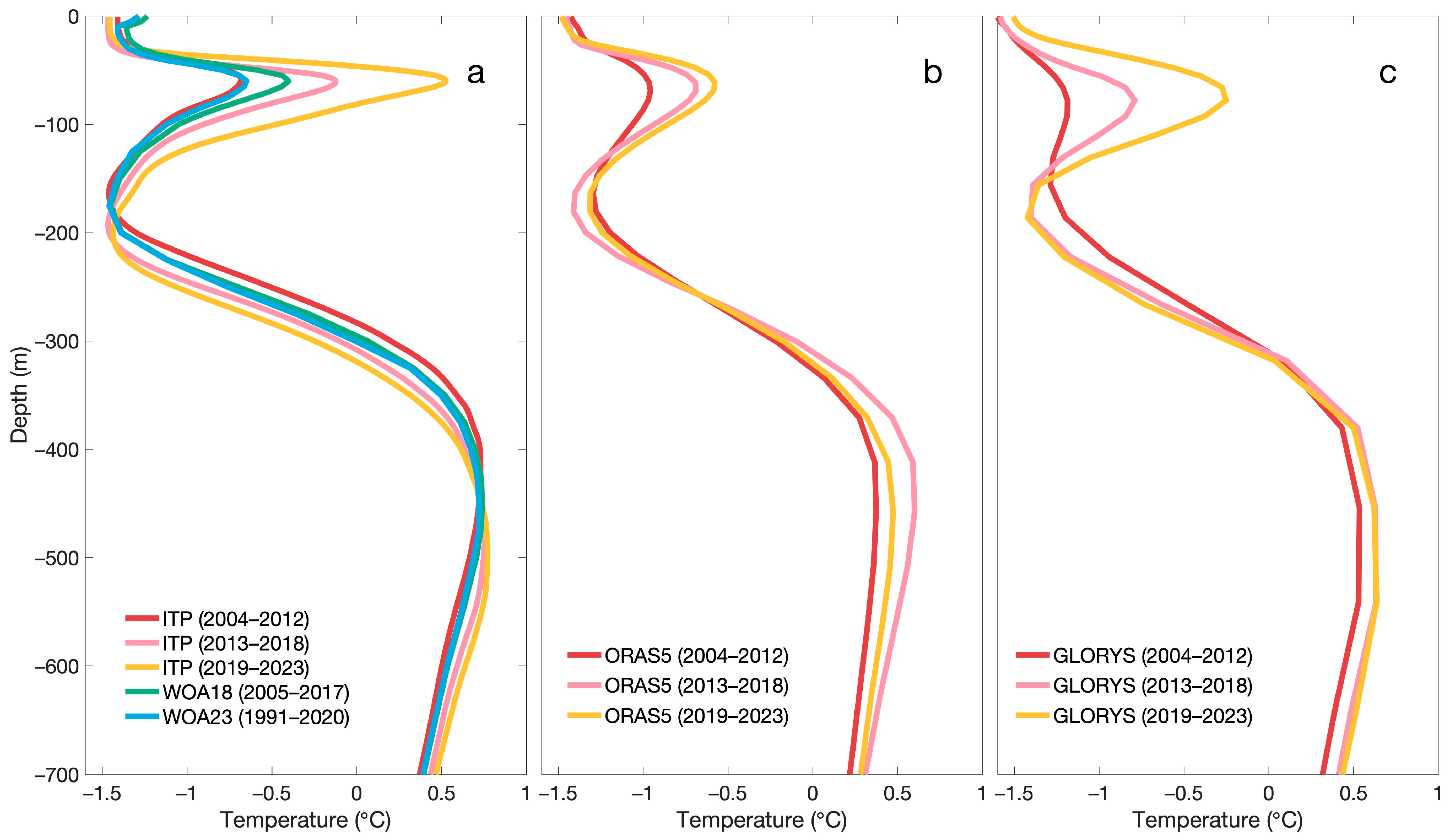
The phased (2004–2012, 2013–2018, and 2019–2023) climatological temperature profiles derived from (a) ITP profiles compared to the average temperature profiles extracted from WOA18 (2005–2017) and WOA23 (1991–2020). (b) ORAS5 and (c) GLORYS12V1.
At the successive stages of the 2004–2012, 2013– 2018, and 2019–2023 periods, the temperature of the subsurface Pacific warm water increased. The maximum values were about −0.7 °C (2004–2012), −0.2 °C (2013–2018), and 0.5 °C (2019–2023), respectively. Compared with the climatological profiles extracted from WOA18 (2005–2017) and WOA23 (1991–2020), these three profiles derived from ITPs were within reasonable range values. The upper profile of the 2005–2017 period from WOA18 lied between the profile of the 2004–2012 ITPs and the profile of the 2013–2018 ITPs. The upper profile of the 1991–2020 period from WOA23 was in agreement with the profile of the 2004–2012 ITPs. The warming of SPWW resulted in an increase in the OHC.
In the intermediate layer, the maximum temperatures of the Atlantic warm water were about 0.73 °C (2004–2012), 0.75 °C (2013–2018), and 0.77 °C (2019–2023). Although the change in maximum values slightly increased, the IAWW contributed to the OHC due to its large water volume. Additionally, the depth of the maximum value of the IAWW deepened. The depths were about 427 m (2004–2012), 479 m (2013–2018), and 497 m (2019–2023), respectively.
The phased climatological temperature profiles derived from ORAS5 and GLORYS12V1 are shown in Figure 7b,c. The results show that they had the same increasing trend as the ITP observations. However, the reanalysis data significantly underestimated the SPWW and IAWW. For example, over the 2019–2023 period (Table 2), the mean maximum value of the SPWW (IAWW) was about 0.53 °C (0.77 °C) for the ITP observations, while the mean maximum values of the SPWW (IAWW) were about −0.58 °C (0.47 °C) for ORAS5 and −0.25 °C (0.64 °C) for GLORYS12V1. The value of the observational data was higher than that of the reanalysis data. The maximum value depths of the IAWW were 457.6 m for ORAS5 and 541 m for GLORYS12V1, but it varied from 427 to 497 m for the ITP observations from 2004 to 2023. ORAS5 and GLORYS12V1 did not capture the deepening characteristic of the maximum value depth of the IAWW.
Table 2.
The mean maximum temperature values of the SPWW and IAWW and their depths derived from ITP, ORAS5, and GLORYS12V1.
4.3. Prediction of the Temperature Profile Using Bi-LSTM Network
Using the reanalysis data (ORAS5 and GLORYS12V1) and the observational data (ITP), the different variations in SPWW and IAWW from 1993 to 2023 were derived. Due to their contributions to the OHC in the SCB, the future trends of SPWW and IAWW are key issues.
We employed the Bi-LSTM neural network to predict variations in the temperature profiles in the SCB. Details of Bi-LSTM are presented in the Section 3. After removing most of the upper 30 m data, the upper 700 m data from ORAS5, GLORYS12V1, and ITP were averaged over the SCB region (the black box in Figure 3a). We first used monthly ORAS5 and GLORYS12V1 data from January 1993 to December 2022 to train the Bi-LSTM network separately, and then profiles from every twelve consecutive months were used to predict the next month’s profiles for a rolling prediction. To verify the effectiveness of the prediction, we used ORAS5 and GLORYS12V1 data from January 2022 to December 2022 for the 2023 rolling prediction. When comparing the 2023 prediction data and the 2023 real ORAS5 data, it was revealed that the root mean square error was 0.039 °C (0.022 °C) and the mean absolute error was 0.021 °C (0.016 °C) in the upper 30 m (50 m) to 700 m temperature profile. When comparing the 2023 prediction data and the 2023 real GLORYS12V1 data, the root mean square error was 0.053 °C (0.035 °C) and the mean absolute error was 0.032 °C (0.026 °C) in the upper 30 m (50 m) to 700 m temperature profile. The test results show that the predicted data agree very well with the ‘real’ data.
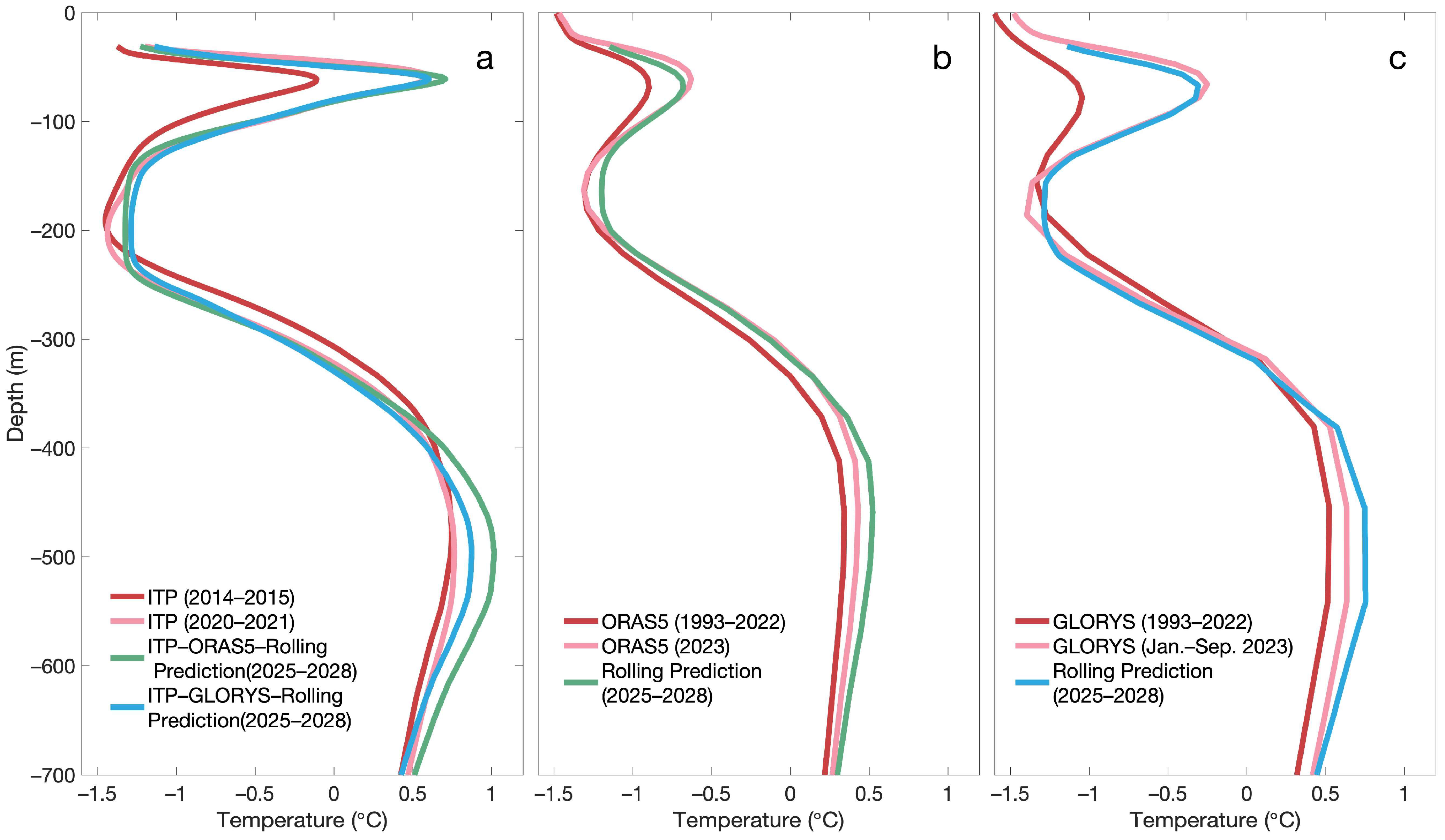
Based on the ORAS5 and GLORYS12V1 training networks mentioned above, four experiments were carried out. Under both training networks, the first two experiments were conducted using the ITP data from January 2021 to December 2021 for the rolling prediction for the January 2022 to December 2028 period. The third experiment was conducted using the ORAS5 training network and the ORAS5 data from October 2022 to September 2023 for the rolling prediction for the October 2023 to December 2028 period. The fourth experiment was conducted using the GLORYS12V1 training network and GLORYS12V1 data from October 2022 to September 2023 for the rolling prediction for the October 2023 to December 2028 period. The rolling prediction profiles are compared with the historical profiles shown in Figure 8. The maximum temperature values and depths of the SPWW and IAWW are presented in Table 3.
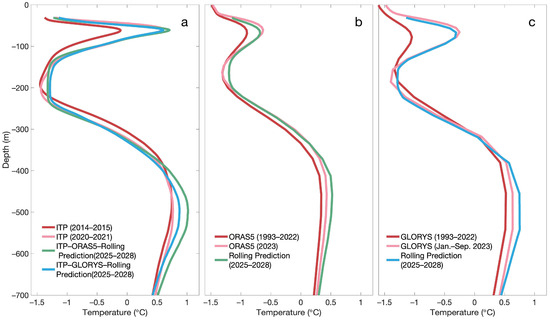
Figure 8.
The rolling prediction of the temperature profiles based on the monthly ORAS5 and GLORYS12V1 training data from January 1993 to December 2022. (a) The comparisons of the ITP profiles averaged from January 2014 to December 2015 and from January 2020 to December 2021, and the rolling prediction profiles averaged from January 2025 to December 2028. The monthly ITP data from January 2021 to December 2021 were used for the prediction. (b) The comparisons of the ORAS5 profiles averaged from January 1993 to December 2022, January 2023 to December 2023 and the rolling prediction profiles from January 2025 to December 2028. The monthly ORAS5 data from January 2022 to December 2022 were used for the prediction. (c) The comparisons of the GLORYS12V1 profiles averaged from January 1993 to December 2022 and from January 2023 to September 2023 and the rolling prediction profiles from January 2025 to December 2028. The monthly GLORYS12V1 data from January 2022 to December 2022 were used for the prediction.
Table 3.
The rolling prediction of the mean maximum temperature values of the SPWW and IAWW and their depths.
Averaged over the forecast period of 2025 to 2028, there is no noticeable change in the SPWW. Changes are mainly seen in the IAWW. In the four rolling prediction experiments, the maximum values of IAWW reach about 1.02 °C (ITP-ORAS5), 0.87 °C (ITP-GLORYS12V1), 0.52 °C (ORAS5), and 0.75 °C (GLORYS12V1), respectively. When averaged over the recent period from 2019 to 2023, the maximum values of the IAWW were about 0.77 °C (ITP), 0.47 °C (ORAS5), and 0.64 °C (GLORYS12V1). The temperature of the IAWW will significantly increase. The depths of the maximum values of SPWW and IAWW are almost not changed. It can be predicted that the OHC in the upper ocean will increase due to the warming of the IAWW.
5. Discussion and Conclusions
The IAWW and SPWW mainly contribute to the upper OHC in the SCB. Based on the reanalysis data (ORAS5 and GLORYS12V1) and observational data (WOA and ITP), the SPWW significantly warmed in the SCB from 1993 to 2023. The temperature increase in the IAWW is smaller than that in the SPWW, but the IAWW has a larger volume and larger temperature value. Small changes in the IAWW will cause significant changes in the OHC. Both the temperature increases in the SPWW and IAWW induced the OHC increase in the Southern CB.
Although the reanalysis data (ORAS5 and GLORYS12V1) capture the temperature’s increasing trend in the SPWW and IAWW, the amplitude was significantly underestimated. In the 2004–2012, 2013–2018, and 2019–2023 periods, the mean maximum value of SPWW (IAWW) for the ORAS5 and the GLORYS12V1 was below that of the ITP observations. In addition, the reanalysis data did not capture the deepening characteristic of the maximum value depth of the IAWW. The bias in the temperature simulation led to a significant underestimation of the OHC in the reanalysis modeling.
Based on the ITP rolling prediction from the Bi-LSTM neural network, the maximum temperature of the IAWW could extend to 1.02 °C from 2025 to 2028. This means that the intrusion of the North Atlantic water into the Arctic Ocean will continue to intensify in the future, and the upper OHC will continue to increase in the SCB. The OHC plays an important role in the freezing and melting of the sea ice. The underestimation of the OHC in the reanalysis data will affect the accuracy of the sea ice simulation. This suggests that there is a potentially large source of error for existing climate models in modeling Arctic sea ice variability, specifically in modeling the heat content of the upper Arctic Ocean well.
Our study focused on the increase in the upper OHC and the variations in the vertical temperature profiles. Importantly, ocean dynamic processes could induce the upward heat transfer from the IAWW and to SPWW. The halocline layer governs the communication between the interior of the Arctic Ocean and the upper ocean and ice cover [16]. In the CB, the enhanced shortwave solar radiation and anticyclonic wind fields result in a significant decrease in the surface salinity [17]. Although the freshening of the upper layer and the strengthening of the halocline hinder the upward heat transfer from the lower warm water, we speculate that the subsurface eddy processes could contribute to the ventilation of the halocline and the upward heat transfer. In the sea ice margins of the Arctic Ocean, eddies are able to “trap” fragmented sea ice. Cyclonic eddies bring relatively warm subsurface waters into the mixing layer, and the sea ice melts more quickly. Surface eddies can accelerate the retreat of the summer sea ice edge by 1–2 km/day [18]. Whether or not ocean processes, such as eddies, are considered can have a significant impact on the bias of sea ice forecasts [19].
Increasing the ocean model resolution may significantly improve the simulation of spatial and temporal variations in the Arctic Ocean sea ice area and volume [20]. As the resolution of the ocean model increases, it is possible to improve the simulation of small- and medium-scale processes, including ocean eddies. The submesoscale processes within eddies would induce the mixing effect across density thermoclines [21] and induce vertical heat transport [22]. This would further improve the modeling of the interactions between the ocean and sea ice. Therefore, improving the resolution of the ocean model should be the main focus of a coupled ocean-ice–atmosphere model. This will be investigated in our future work.
Author Contributions
Conceptualization, Y.L.; funding acquisition, Y.L.; methodology, C.Y. and H.C.; project administration, Y.L.; validation, Y.L.; visualization, Y.L. and C.Y.; writing—original draft, Y.L.; writing—review and editing, X.L. and G.H. All authors have read and agreed to the published version of the manuscript.
Funding
This study was supported by the Natural Science Foundation of China Project (No. 42376004 and 42206005), the Southern Marine Science and Engineering Guangdong Laboratory (Zhuhai) (Grant SML2020SP007), and the National Key Research and Development Program of China (2018YFA0605904).
Institutional Review Board Statement
Not applicable.
Informed Consent Statement
Not applicable.
Data Availability Statement
Data are contained within the article.
Conflicts of Interest
The authors declare no conflicts of interest.
References
- Liu, Z.; Risi, C.; Codron, F.; Jian, Z.; Wei, Z.; He, X.; Poulsen, C.J.; Wang, Y.; Chen, D.; Ma, W.; et al. Atmospheric forcing dominates winter Barents-Kara sea ice variability on interannual to decadal time scales. Cryosphere 2022, 119, e2120770119. [Google Scholar] [CrossRef] [PubMed]
- Topál, D.; Ding, Q. Atmospheric circulation-constrained model sensitivity recalibrates Arctic climate projections. Nat. Clim. Chang. 2023, 13, 710–718. [Google Scholar] [CrossRef]
- Polyakov, I.; Alekseev, G.; Timokhov, L.; Bhatt, U.; Colony, R.; Simmons, H.; Walsh, D.; Walsh, J.; Zakharov, V.F. Variability of the intermediate Atlantic water of the Arctic Ocean over the last 100 years. J. Clim. 2004, 17, 4485–4497. [Google Scholar] [CrossRef]
- Polyakov, I.V.; Pnyushkov, A.V.; Alkire, M.B.; Ashik, I.M.; Alexander, Y.L. Greater role for Atlantic inflows on sea-ice loss in the Eurasian Basin of the Arctic Ocean. Science 2017, 356, 285–291. [Google Scholar] [CrossRef] [PubMed]
- Lin, L.; Lei, R.; Hoppmann, M.; Perovich, D.K.; He, H. Changes in the annual sea ice freeze–thaw cycle in the Arctic Ocean from 2001 to 2018. Cryosphere 2022, 16, 4779–4796. [Google Scholar] [CrossRef]
- Timmermans, M.-L.; Toole, J. The Arctic Ocean’s Beaufort Gyre. Annu. Rev. Mar. Sci. 2023, 15, 223–248. [Google Scholar] [CrossRef] [PubMed]
- Shi, J.; Zhao, J.; Li, S.; Cao, Y.; Qu, P. A double-halocline structure in the Canada Basin of the Arctic Ocean. Acta Oceanol. Sin. 2005, 24, 25. [Google Scholar]
- Toole, J.M.; Timmermans, M.L.; Perovich, D.K.; Krishfield, R.A.; Proshutinsky, A.; Richter-Menge, J.A. Influences of the ocean surface mixed layer and thermohaline stratification on Arctic Sea ice in the central Canada Basin. J. Geophys. Res.-Ocean. 2010, 115, C10018. [Google Scholar] [CrossRef]
- Jean-Michel, L.; Eric, G.; Romain, B.-B.; Gilles, G.; Angélique, M.; Marie, D.; Clément, B.; Mathieu, H.; Olivier, L.G.; Charly, R.; et al. The Copernicus Global 1/12° Oceanic and Sea Ice GLORYS12 Reanalysis. Front. Earth Sci. 2021, 9, 698876. [Google Scholar] [CrossRef]
- Cheng, L.; Abraham, J.; Zhu, J.; Trenberth, K.E.; Fasullo, J.; Boyer, T.; Locarnini, R.; Zhang, B.; Yu, F.; Wan, L. Record-setting ocean warmth continued in 2019. Adv. Atmos. Sci. 2020, 2, 137–142. [Google Scholar] [CrossRef]
- Hochreiter, S.; Schmidhuber, J. Long short-term memory. Neural Comput. 1997, 9, 1735–1780. [Google Scholar] [CrossRef] [PubMed]
- Ahmed, M.; Mumtaz, R.; Anwar, Z.; Shaukat, A.; Arif, O.; Shafait, F. A multi–step approach for optically active and inactive water quality parameter estimation using deep learning and remote sensing. Water 2022, 14, 2112. [Google Scholar] [CrossRef]
- Jia, X.; Ji, Q.; Han, L.; Liu, Y.; Han, G.; Lin, X. Prediction of Sea Surface Temperature in the East China Sea Based on LSTM Neural Network. Remote Sens. 2022, 14, 3300. [Google Scholar] [CrossRef]
- Luo, Q.-R.; Xu, H.; Bai, L.-H. Prediction of significant wave height in hurricane area of the Atlantic Ocean using the Bi-LSTM with attention model. Ocean Eng. 2022, 266, 112747. [Google Scholar] [CrossRef]
- Jiang, F.; Ma, J.; Wang, B.; Shen, F.; Yuan, L. Ocean observation data prediction for Argo data quality control using deep bidirectional LSTM network. Secur. Commun. Netw. 2021, 2021, 5665386. [Google Scholar] [CrossRef]
- Polyakov, I.V.; Pnyushkov, A.V.; Carmack, E.C. Stability of the arctic halocline: A new indicator of arctic climate change. Environ. Res. Lett. 2018, 13, 125008. [Google Scholar] [CrossRef]
- Dong, J.; Jin, M.; Liu, Y.; Dong, C. Interannual variability of surface salinity and Ekman pumping in the Canada Basin during summertime of 2003–2017. J. Geophys. Res.-Ocean. 2021, 126, e2021JC017176. [Google Scholar] [CrossRef]
- Johannessen, J.; Johannessen, O.; Svendsen, E.; Shuchman, R.; Manley, T.; Campbell, W.; Josberger, E.; Sandven, S.; Gascard, J.; Olaussen, T. Mesoscale eddies in the Fram Strait marginal ice zone during the 1983 and 1984 Marginal Ice Zone Experiments. J. Geophys. Res.-Ocean. 1987, 92, 6754–6772. [Google Scholar] [CrossRef]
- Manucharyan, G.E.; Thompson, A. Submesoscale sea ice-ocean interactions in marginal ice zones. J. Geophys. Res.-Ocean. 2017, 122, 9455–9475. [Google Scholar] [CrossRef]
- Docquier, D.; Grist, J.P.; Roberts, M.J.; Roberts, C.D.; Semmler, T.; Ponsoni, L.; Massonnet, F.; Sidorenko, D.; Sein, D.V.; Iovino, D. Impact of model resolution on Arctic sea ice and North Atlantic Ocean heat transport. Clim. Dynam. 2019, 53, 4989–5017. [Google Scholar] [CrossRef]
- Sun, W.; Dong, C. Isopycnal and diapycnal mixing parameterization schemes for submesoscale processes induced by mesoscale eddies. Deep-Sea Res. II 2022, 202, 105139. [Google Scholar] [CrossRef]
- Wang, Q.; Dong, C.; Dong, J.; Zhang, H.; Yang, J. Submesoscale processes-induced vertical heat transport modulated by oceanic mesoscale eddies. Deep-Sea Res. II 2022, 202, 105138. [Google Scholar] [CrossRef]


Disclaimer/Publisher’s Note: The statements, opinions and data contained in all publications are solely those of the individual author(s) and contributor(s) and not of MDPI and/or the editor(s). MDPI and/or the editor(s) disclaim responsibility for any injury to people or property resulting from any ideas, methods, instructions or products referred to in the content. |
© 2024 by the authors. Licensee MDPI, Basel, Switzerland. This article is an open access article distributed under the terms and conditions of the Creative Commons Attribution (CC BY) license (https://creativecommons.org/licenses/by/4.0/).