Four Storm Surge Cases on the Coast of São Paulo, Brazil: Weather Analyses and High-Resolution Forecasts

Abstract

The coast of São Paulo, Brazil, is exposed to storm surges that can cause damage and floods. These storm surges are produced by slowly traveling cyclone–anticyclone systems. The motivation behind this work was the need to evaluate high-resolution forecasts of the mean sea-level pressure and 10 m winds, which are the major drivers of the wave model. This work is part of the activity in devising an early warning system for São Paulo coastal storm surges. For the evaluation, four case studies that had a major impact on the coast of São Paulo in 2020 were selected. Because storm surges that reach the coast may cause coastal flooding, precipitation forecasts were also evaluated. The mesoscale Eta model produces forecasts with a 5 km resolution for up to an 84 h lead time. The model was set up in a region that covers part of southeast and south Brazil. The ERA5 reanalysis was used to describe the large-scale synoptic conditions and to evaluate the weather forecasts. The cases showed a region in common between 35° S, 40° S and 35° W, 45° W where the low-pressure center deepened rapidly on the day before the highest waves reached the coast of São Paulo, with a mostly eastward, rather than northeastward, displacement of the associated surface cyclone and minimal or no tilt with height. The winds on the coast were the strongest on the day before the surge reached the coast of São Paulo, and then the winds weakened on the day of the maximum wave height. The pattern of the mean sea-level pressure and 10 m wind in the 36 h, 60 h, and 84 h forecasts agreed with the ERA5 reanalysis, but the pressure was slightly underestimated. In contrast, the winds along the coast were slightly overestimated. The 24 h accumulated precipitation pattern was also captured by the forecast, but was overestimated, especially at high precipitation rates. The 36 h forecasts showed the smallest error, but the growth in the error for longer lead times was small, which made the 84 h forecasts useful for driving wave models and other local applications, such as an early warning system.

1. Introduction

The coast of São Paulo is located between the latitudes of 23°15′ S and 25°15′ S, and is a typical subtropical region. The region encompasses sixteen cities and several economic activities, such as offshore oil and gas production, the Santos Port Complex, tourism, and industries. It also has conservation areas for the remains of the native forest, Mata Atlantica. The total population of the coastal area exceeds 2.2 million [1].

Southerly extratropical cyclones and anticyclones travel toward this region, and they either divert eastward, decelerate their motion, or stall. These phenomena are often responsible for causing storm surges that can reach the coast of São Paulo. The permanent anticyclone over the Southern Atlantic Ocean can affect the progression of these transient systems, which affects the intensity and duration of storm surges. The atmospheric conditions that lead to the extreme wave events generated by extratropical cyclones in the southwestern portion of the South Atlantic Ocean have been studied by Gramcianinov et al. [2]. These authors showed that extreme waves can occur in three regions of extratropical cyclones: behind the cold front, along the warm front, and ahead of the cold front. The authors pointed out that the anticyclone position relative to the cyclone center plays an important role in extreme waves. An increase in the horizontal pressure gradient causes stronger wind speeds, producing higher waves.

Based on a long-term record database of severe and extreme storm surge events (1928–2021), the authors of [3,4] showed that storm surges and tidal surges that reach the coast of São Paulo have become more frequent and stronger in intensity and magnitude in the present century. These surges have caused severe coastal erosion and coastal flooding that has resulted in serious damage to the coastal infrastructure and disruptions to all livelihoods.

Sondermann et al. [5] identified the atmospheric patterns that are favorable for storm surges on the coast of São Paulo. These patterns are primarily based on the sea-level pressure and the intensity and direction of 10 m winds. The authors used data from the ERA5 reanalysis for May from 1981 to 2010. The results indicated the occurrence of three atmospheric patterns. Pattern 1 was the least frequent and was characterized by a coastal low-pressure center and southwesterly winds parallel to the coast. Pattern 2 featured a wide wind fetch created by a high-pressure center south of the South Atlantic Ocean and a low-pressure center to the north, resulting in intense winds that transported moisture to the coast, causing increased rainfall along the coast of Santos. Pattern 3 was marked by southwesterly winds originating from continental high pressure and oceanic troughs. This atmospheric configuration led to intense winds along the coastline, resulting in high waves and tides caused by bad weather.

Future changes in the frequency and intensity of these storm surges will raise the risk of disasters. According to Sondermann et al. [6], based on the Eta regional model’s downscaling of the Brazilian Earth System Model’s (BESM’s) [7] projections for RCP4.5 and RCP8.5 greenhouse gas scenarios, the storm surge events characterized by pattern 1 are expected to become more intense. However, these events will continue to be the least frequent in the future. For pattern 2, both RCP scenarios indicated a decrease in the number of events, but with increased precipitation along the coastline. The combination of heavy rain and strong winds may lead to a higher risk associated with storm surge events. Pattern 3 presented no change in the storm surge frequencies in the future, but the winds tended to be weaker. Chou et al. [8] analyzed the surface pressure on the São Paulo coast and found a trend towards weakening of low-pressure systems in the future climate. Armani et al. [9] calculated the projections of extreme precipitation indices for the São Paulo state. They concluded that, while the precipitation was projected to decrease in most parts of the state, along the coastal region, the total annual precipitation was projected to increase in the near future.

A web-based platform has been devised for the monitoring and early warning of storm surge events impacting the coast of São Paulo [10]. This platform was preceded by two important storm surge early warning systems. The first was developed for the city of Santos [11,12], which is the most populous city on the coast of São Paulo and is historically very susceptible to impacts resulting from extreme meteorological and oceanographic events. The second was developed for the Santos metropolitan region [13], which includes the city of Santos and eight other coastal cities.

The platform SARIC (in Portuguese, the acronym stands for early warning system of storm surges and coastal flooding) contains 4-day forecasts that include the significant wave height, peak wave period, and mean wave direction, as well as the sea level for several points near the coast of São Paulo. These are products from nested grids, implemented using Delft3D-FLOW [14] and Delft3D-WAVE [15], with a spatial resolution of between 500 m and 5 km. As boundary conditions, the set of hydrodynamic models uses the astronomical tides obtained from the global tide model TOPEX/POSEIDON Global Inverse Solution (TPXO 7.2) [16] and the temperature, salinity, sea level, and current data from the Global Ocean Sea Physical Analysis and Forecast service [17], provided by the Copernicus Marine Service (CMS). The set of wave models uses the spectral results from the CMS global wave model [18]. The atmospheric high-resolution Eta model drives both the hydrodynamic and wave model [19,20] forecasts, which are driven by the GFS model forecasts. The daily forecasts and the early warning system are applied to every beach on the coast of São Paulo. All numerical model forecasts contain errors; in a nested system, the Eta model’s forecast errors can propagate into the ocean-wave modeling systems. When devising the forecast system, the following questions were posed: How well does the atmospheric modeling system forecast the mean sea-level pressure and the 10 m winds? Is the skill of these forecasts useful for driving the wave models on the coast of São Paulo? For which forecast lead time are the forecasts more skillful?

Therefore, the objective of this work was to evaluate the skill of the Eta-GFS modeling system in forecasting the mean sea-level pressure and 10 m winds, which are the major drivers of the wave model. The Eta atmospheric model and the Delft3D wave model are part of a storm surge and coastal flood monitoring system under development. In addition, the large-scale meteorological conditions of four major cases that occurred in 2020 are described. Since the storm surges that reach the coast are accompanied by coastal flooding, precipitation forecasts were also evaluated.

This article is organized as follows: the choice of the cases and a description of the Eta model are provided in Section 2; a description of the atmospheric large-scale conditions during the peaks of the storm surge events and an evaluation of the forecasts of these events are given in Section 3 (Results); and the Discussion and Conclusions make up Section 4 and Section 5, respectively.

2. Materials and Methods

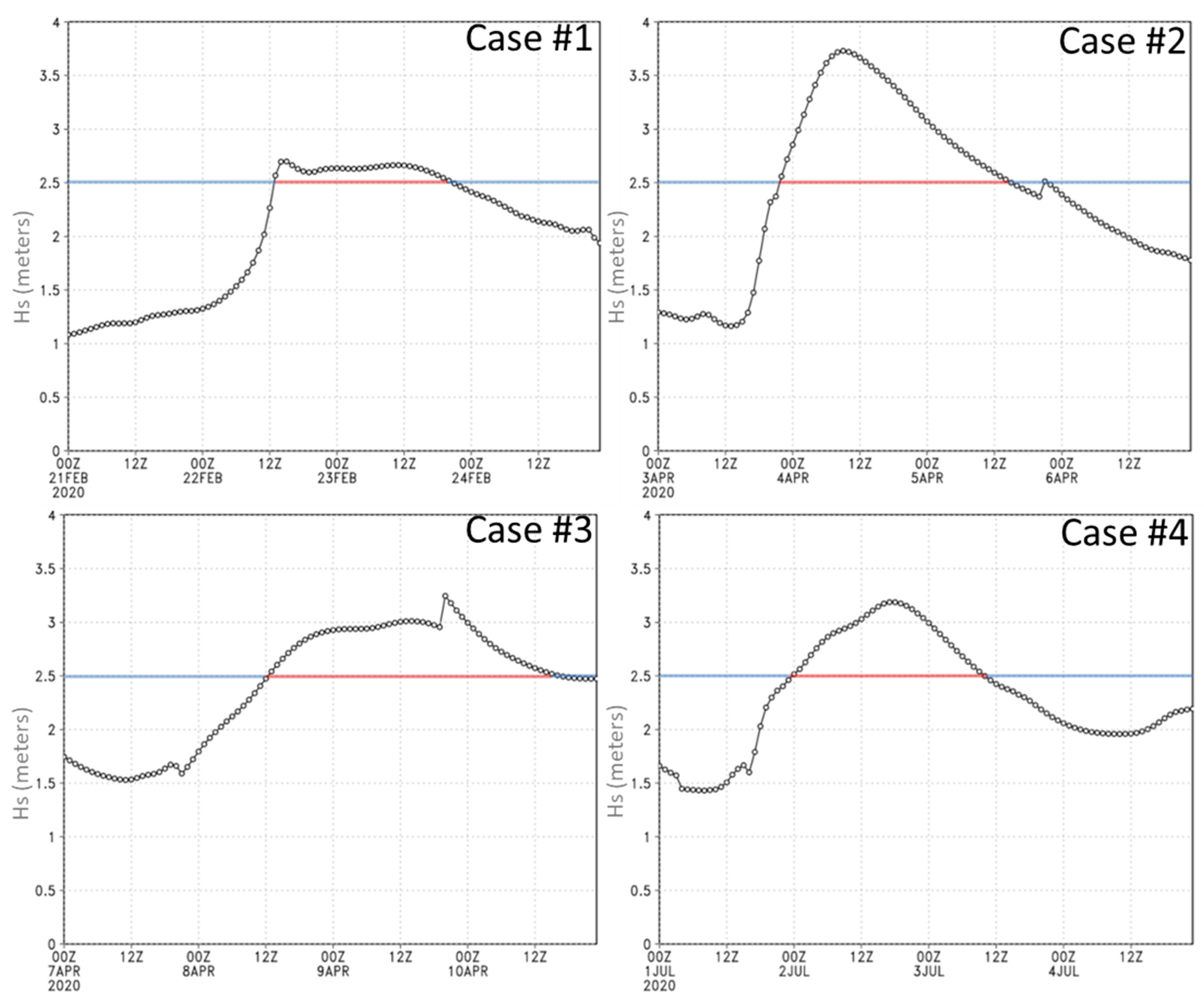
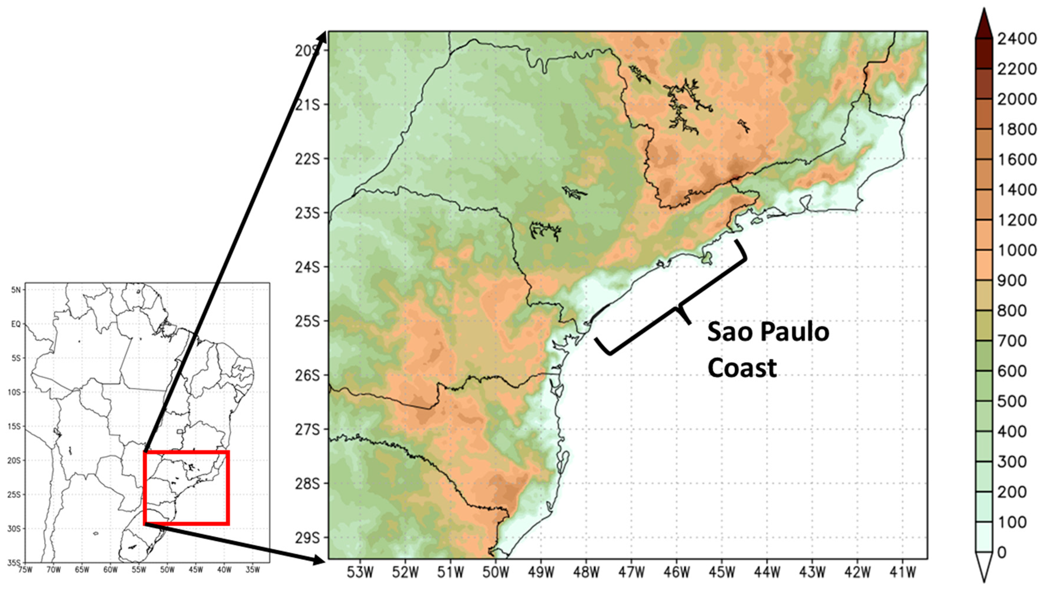
2.1. The Storm Surge Cases

Four case studies of storm surges (

Table 1. Description of the four cases in this study. The bold dates indicate the dates on which the highest waves were registered.

Case #	Peak Date of the Event	Type of Storm Surge Event
1	22 and 23 February 2020	Storm tide + rough sea
2	4 and 5 April 2020	Storm tide + rough sea
3	8 and 9 April 2020	Storm tide + rough sea
4	2 and 3 July 2020	Rough sea

) were selected from the database of storm surge events for the São Paulo coast [4], as those cases caused major impacts on the coast in 2020. The impacts on the beaches along the entire coastline were documented. According to the authors of [3], three types of storm surge events, from severe to extreme, reach the São Paulo coast, causing different kinds of impacts as follows:

• Severe events (very rough sea): These are characterized by strong to extremely strong waves. The primary impact is coastal and beach erosion, with only localized coastal flooding.
• Severe events (storm tide): These events are characterized by a combination of storm surges and high tides [21]; the worst scenario occurs when a strong storm surge coincides with the spring tide peak, resulting in higher storm tides. The primary impact is coastal flooding along the seafront, with less beach erosion.
• Extreme events (storm tide + rough sea): These events occur when both types of severe events occur simultaneously. They cause significant coastal erosion and major coastal flooding along both the seafront and estuarine/lagoonal shorelines, especially when associated with heavy rainfall.

In summary, “severe” events are characterized by either strong waves or high sea levels, causing either erosion or flooding. In contrast, “extreme” events involve both strong waves and high sea levels, leading to both significant erosion and major flooding.

The significant wave height (Hs) time series was taken from a point located just offshore of the city of Santos (24.13° S, 45.68° W), which is approximately halfway along the coast of São Paulo. The Hs from the ERA5 [22] dataset for the different cases is shown in Figure 1. The Brazilian Navy adopts a threshold of 2.5 m for the storm wave height in the open sea.

In terms of hydrodynamic patterns, the mean amplitudes of the sea level, particularly measured in the Santos Port Channel, are 1.17 m and 0.26 m in the spring and neap tides, respectively; passages of cold fronts are frequent in this region, mainly in the winter season, and they produce variations in the sea level that can exceed 0.8 m [11,12].

In case #1, during the spring tide, the wave heights started to rise fast after 09Z, 22 February 2020, from about 1.5 m to just over 2.5 m at 12Z. This height was nearly constant for about 24 h and started to decrease slowly after 00Z, 24 February 2020. The waves were just over 2.5 m for about 30 h. The impacts of this case on the coast of São Paulo were mainly associated with coastal flooding on the beaches and some stretches of the coastline at the beginning of the afternoon on 23 February.

In case #2, at neap tide, the wave heights climbed fast after 14Z, 3 April 2020, from about 1.5 m to a peak of over 3.5 m at 09Z, 4 April 2020. The peak did not last long, and a couple of hours later the wave heights started to slowly decrease after 00Z, 4 April 2020. At 00Z, 6 April 2020, the waves were about 2 m high. The waves were higher than 2.5 m for about 38 h. The impacts of this event along the São Paulo coast included severe coastal erosion and flooding, causing substantial damage to the coastal infrastructure and private properties, as well as disruptions to several types of services.

Case #3 followed immediately after case #2, after a break of about 2.5 days and during a spring tide. In this case, the wave heights slowly increased from 1.5 m on 12Z, 7 April 2020, and only exceeded 2.5 m after 24 h at 12Z, 8 April 2020. They then reached just over 3.0 m after 30 h at 18Z, 9 April 2020. These waves were higher than 2.5 m for about 48 h. Although this event was as intense as case #2, its impacts on the São Paulo coast were greatly magnified, as the beaches were more vulnerable due to the strong erosion suffered during the previous event, causing even more destruction on the shore and greater coastal area flooding.

In case #4, at neap tide, the wave heights slowly climbed after 12Z, 1 July 2020, from about 1.5 m to a peak of over 3.0 m at 18Z, 2 April 2020. This peak did not last long, and soon the wave heights decreased to 2.0 m at 00Z, 4 July 2020. The waves were higher than 2.5 m for about 34 h. This event was marked by wind gusts and very strong waves, which disrupted the Port of Santos by causing the sinking of small boats in some areas, falling trees, and the destruction of urban structures and private properties on the seafront, but only on beaches with a high or very high risk of erosion.

2.2. Eta Model Setup

A wave model provides a forecast of storm surges and the sea state in general. Forecasts of atmospheric conditions—in particular, winds and the mean sea-level pressure—are needed as inputs to drive the wave model. In this work, high-resolution weather forecasts for the coast of São Paulo were produced using the Eta model [19,20]. The Eta is a grid-point mesoscale model whose major characteristic is the vertical η-coordinate (35), which names the model and is defined as follows:

$$\eta =\left(\frac{p-p_T}{p_s-p_T}\right)\left[\frac{p_{ref}\left(z_s\right)-p_T}{p_{ref}\left(0\right)-p_T}\right]$$

(1)

where p is the pressure; the subscripts T and S refer to the model’s top and surface, respectively; subscript ref refers to a reference atmosphere; and z_s is the model topography height.

This vertical coordinate feature is suitable for application in regions with a complex topography, where the coordinate surfaces remain approximately horizontal, even over areas of sloping terrain, as opposed to the terrain-following vertical coordinate feature adopted by most atmospheric models. The approximately horizontal surfaces of the vertical η-coordinate feature reduce the errors in the calculation of the horizontal pressure gradient force. The Eta model solves the equations in a finite-volume and E-grid discretization, with conservation in the transformation between kinetic and potential energy. It uses a two-level time scheme. The model equations, the grid system, the discretization, and other model details can be found in the work by Mesinger et al. [19] and Gomes et al. [20]. The non-hydrostatic processes are included through a switch [23]. The model has a full physics representation. The convective parametrization is solved using the Betts–Miller–Janjic scheme [24,25], and the cloud microphysics are solved using the Ferrier scheme [26]. The longwave radiation [27] and shortwave radiation [28] schemes are used separately to solve the atmospheric radiative transfer. The land biosphere–atmosphere interactions are solved using the NOAH land surface scheme [29]. Turbulent kinetic energy is a prognostic variable obtained from the Mellor–Yamada level 2.5 scheme [30]. In the surface layer, over the continent, the variables follow Monin–Obukhov theory and use Paulson stability functions [31]; over the ocean, a viscous sublayer is added [25], and the roughness length follows [32].

The model was set as non-hydrostatic for a 5 km resolution in the domain of about 10 degrees in latitude and 13 degrees in longitude, which covered the Sao Paulo coast, as shown in Figure 2. The model had 50 vertical layers, and the model top was set to 25 hPa. The initial and lateral boundary conditions used the NCEP global forecasting system [33] for a 25 km resolution. The Eta model forecasts updated the lateral boundaries every 6 h. The evaluated forecast lead times were up to 84 h.

3. Results

The large-scale atmospheric conditions of these four cases were based on the ERA5 reanalysis data. The Eta model forecasts the local conditions. These forecasts were evaluated against the ERA5 reanalysis and observations.

3.1. Observations

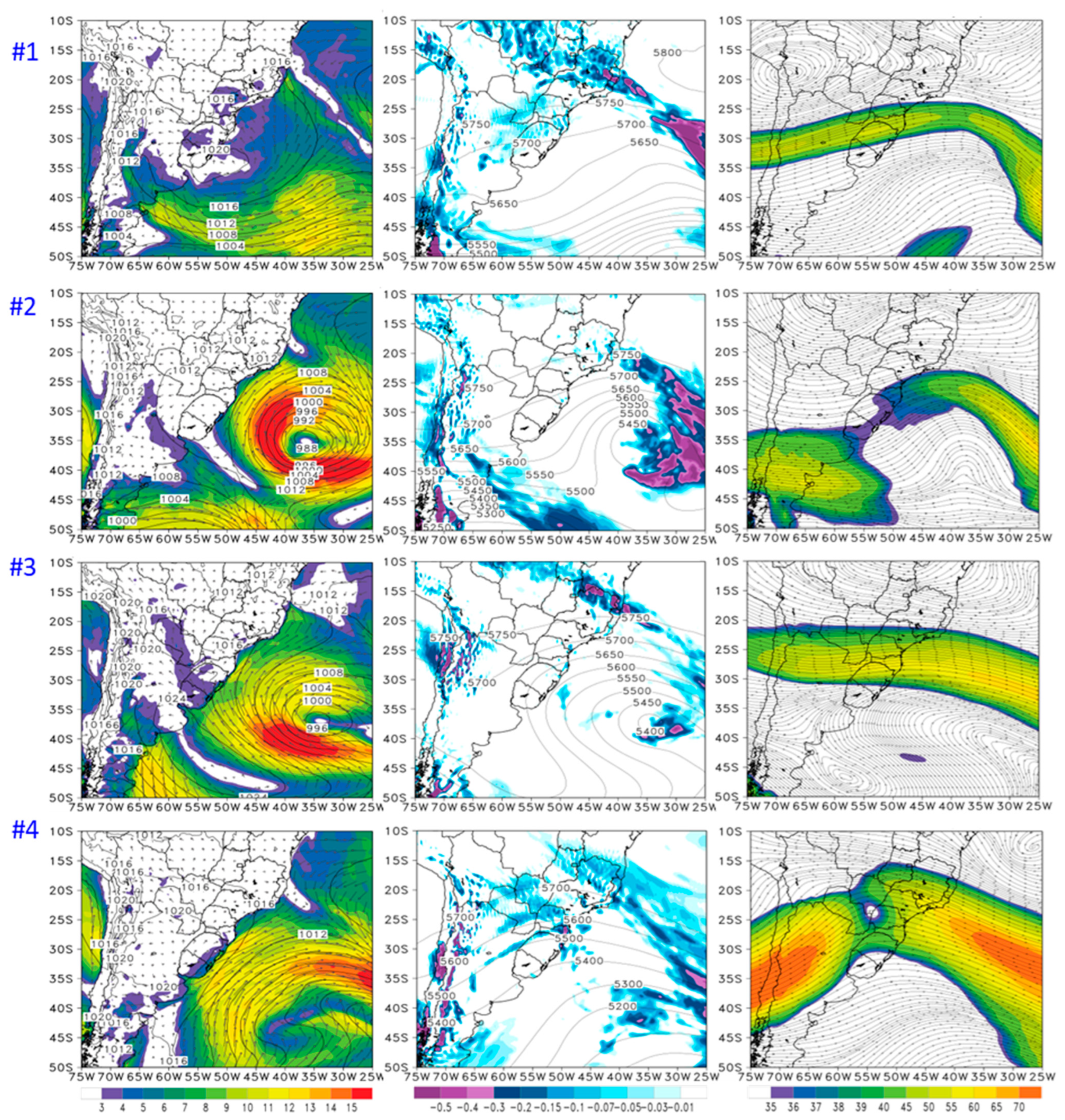
Large-Scale Meteorological Conditions

The synoptic conditions of the selected case studies, based on the mean sea-level pressure (MSLP), 10 m winds, a 500 hPa geopotential height, a 500 hPa upward motion, and 200 hPa winds, are shown in Figure 3.

On 21 February 2020, a low-pressure center was located at about 45° S, 45° W, off the coast of Argentina. Case #1 started on 22 February 2020 (Figure 3), when the wave heights increased quickly and reached their peak of over 2.5 m. The low pressure started to weaken and displace eastward, and then the strongest winds from the western part of the low-pressure area reached the coast of São Paulo, causing damage to the coast. The wave height peaked on 23 February, when the large-scale pattern featured a high-pressure area centered at about 35° S, 50° W, blowing out winds anticyclonically. The winds weakened and reached São Paulo perpendicular to the coast. As a result of the rapid wave run-up associated with the high tide, the beaches were flooded by the sea, catching the crowds. The wind convergence zone extended from the coastal area at about 17° S, which indicates the position of a cold front (middle column in Figure 3). At mid-levels, the strongest upward air motions confirmed the position of the cold front. The axis of the mid-level trough was just to the north of the coast of São Paulo. At the upper levels, the jet stream acquired a cyclonic curvature just off the coast of São Paulo. The large-scale meteorological pattern was of type III according to the Sondermann et al. [5] classification.

Case #2 started on 4 April 2020, when a deep, low-pressure center occurred off the coast of Sao Paulo, centered at about 35° S, 35° W. This low pressure was located at about the same position as on the previous day, when waves started to pile high, and peaked at up to 3.7 m on 4 April 2020. As a result of these strong waves and storm tides, the beaches suffered erosion, and there was coastal flooding all along the coast of São Paulo. This case was a combined event of a storm surge and a tidal surge. However, as it occurred during the lockdown due to the COVID-19 pandemic, the damage mainly occurred to urban infrastructures. The strongest winds blew around the western and southern parts of this low pressure. As the low pressure slowly displaced eastward, those strong winds on the western part of the low-pressure area reached the coast of São Paulo, with southwesterlies along the coast. The wind convergence zone extended from the coastal area at 17° S in the NW–SE direction, where upward motion was maximized at the mid-levels, which indicated the position of a cold front on the coast. At the upper levels, the jet stream showed a cyclonic curvature. On the day of the wave height peaks, the extratropical system was in a mature phase, with the cyclone phase in the troposphere. The large-scale meteorological pattern was of type II according to the Sondermann et al. [5] classification.

Case #3 started on 7 April 2020, when a low-pressure center formed at about 42° S, 43° W, leading to a new event two days after case #2, when waves peaked near the coast again. During the slow eastward displacement of the low pressure, the stronger winds on the western part of the low-pressure area reached the São Paulo coast on 8 April 2020, on the day that the waves started to pile up. Southwesterly winds blew along the coast of São Paulo. The cold front on the day of the wave height peaks was positioned at around 17° S near the coast, as indicated by the mid-level upward motion. This extratropical system was also in the mature phase, but shallower than in the previous case, as the vertical alignment of the cyclone was clearly seen at lower and mid-levels, but at upper levels, the jet stream showed only a weak cyclonic curvature. The impacts on the São Paulo coast were more intense than in case #2, mainly because the beaches were fragile due to the strong erosion caused by the previous event. The large-scale meteorological pattern was of type II according to the Sondermann et al. [5] classification.

In case #4, on 1 July 2020, the low pressure displaced rather fast in a southeastward direction and reached the ocean, where the low pressure deepened substantially in an explosive-cyclogenesis-like pattern, the wave heights increased fast, and strong southwesterly winds reached the coast of São Paulo. On 02 July, a broad area of southwesterlies helped to pile up the waves to reach their greatest heights, although the winds had weakened along the coast. This storm showed some similarity to the previous two cases in April, but this was a winter case, and the low pressure formed over the continent. The winds were the strongest in the northern and southern parts of this low-pressure center. The associated cold front was positioned at about 20° S, as indicated by the lower-level wind reversal from northerly to southwesterly winds and the mid-level upward motion. In addition, the upper-level jet stream had higher speeds, and the cyclonic axis showed some westward tilt with height. The large-scale meteorological pattern was of type II according to the Sondermann et al. [5] classification, because the cyclonic intensification occurred over the ocean.

Among the cases studied, case #1 was the most distinguishable. The coast was under the effects of an anticyclone, with weak winds reaching perpendicular to the coast, the smallest significant wave height, and the largest amounts of precipitation.

3.2. Forecasts

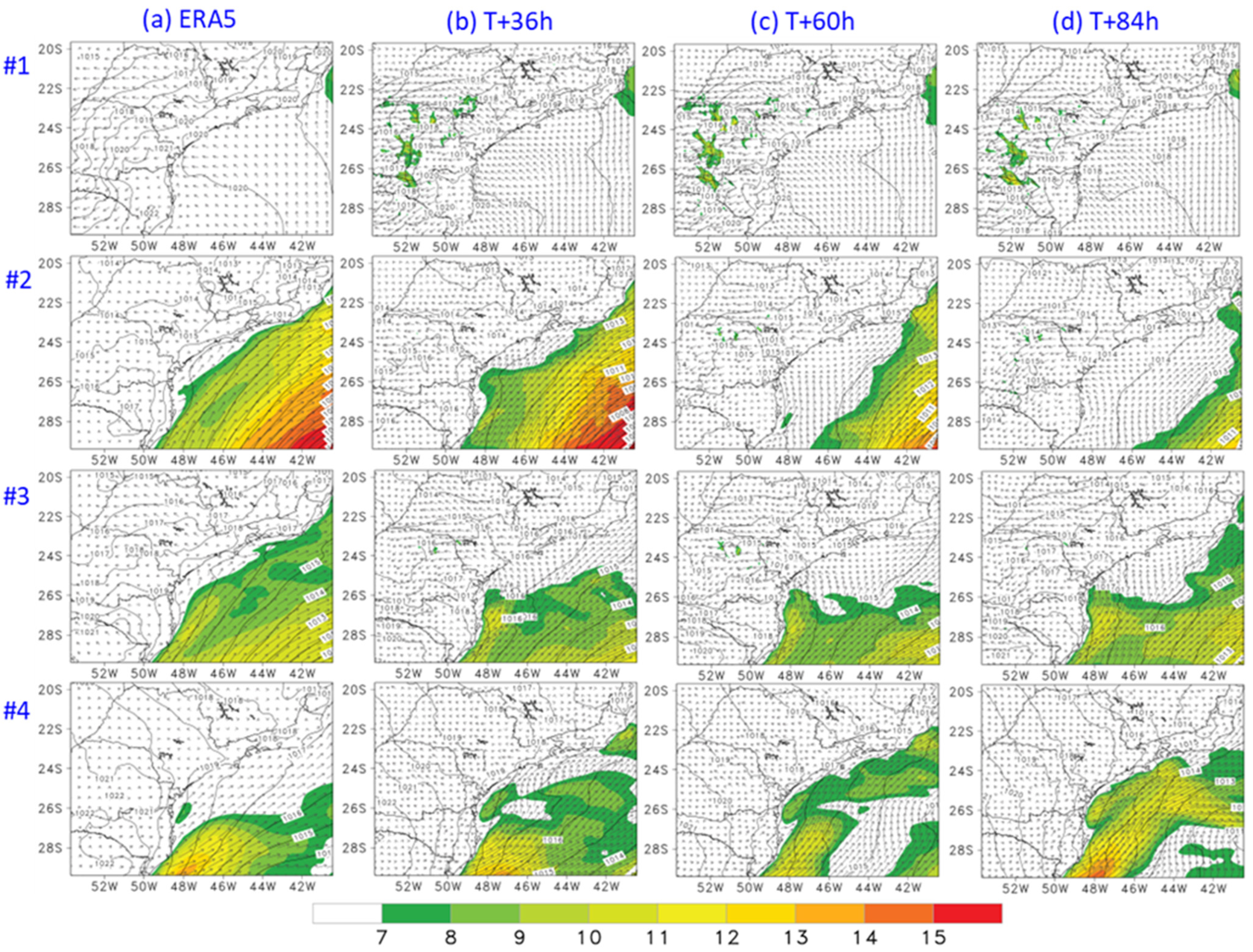
3.2.1. MSLP and 10 m Wind Mesoscale Patterns

Figure 4 shows the MSLPs and the 10-m winds of the four case studies.

In case #1, the flow was perpendicular to the coast and from the ocean toward the land for the 36 h, 60 h, and 84 h forecasts. For the forecast lead times of 36 h and 60 h, the Eta MSLP forecasts reproduced the ERA5 MSLP pattern. However, for the 84-h forecast, the Eta MSLP was lower than the ERA5 MSLP by about 2 hPa. In general, over the ocean, the pressure contours were forecast to be further apart than in the observations, which indicates that the horizontal pressure gradients were slightly weaker in the forecasts.

In case #2, the 36 h forecasts showed the wind blowing correctly from the southwesterly direction and strong wind speeds, similar to the observations. However, for lead times of 60 h and 84 h, the forecasts did not show the southwesterly winds along the coast of São Paulo, and over the ocean, the winds were weaker than in ERA5. Although a pressure value of about 1014 hPa was captured by the forecasts along the coast, away from the coast over the ocean, the forecasts showed fewer pressure contours, which indicates weaker horizontal pressure gradients, and therefore, weaker winds. In this case, the longer the lead time, the weaker the winds over the ocean.

In case #3, the stronger winds were restricted to the southern part of the ocean area of the model domain, whereas ERA5 showed stronger winds over all the ocean areas. Near the coast, the forecast winds generally entered the continent in a southeasterly direction; however, the observations showed the winds blowing strongly and southwesterly. In this case, the Eta MSLP was lower than the ERA5 MSLP by about 2 hPa along the coast of São Paulo.

In case #4, the winds were correctly forecast in the southwesterly direction along the coast of São Paulo, but were too strong, particularly at 84 h. The forecast MSLP was weaker than ERA5, but as the forecast approached the initial conditions, such as the 36 h forecasts, the MSLP was closer to the ERA5 value.

In summary, the 36 h forecast lead time was more accurate than the 60 h and 84 h forecast lead times. Nevertheless, the 84 h forecasts did show patterns that were useful as guidance for the event. The Eta MSLP and its horizontal gradients were generally lower and weaker than the ERA5 reanalysis.

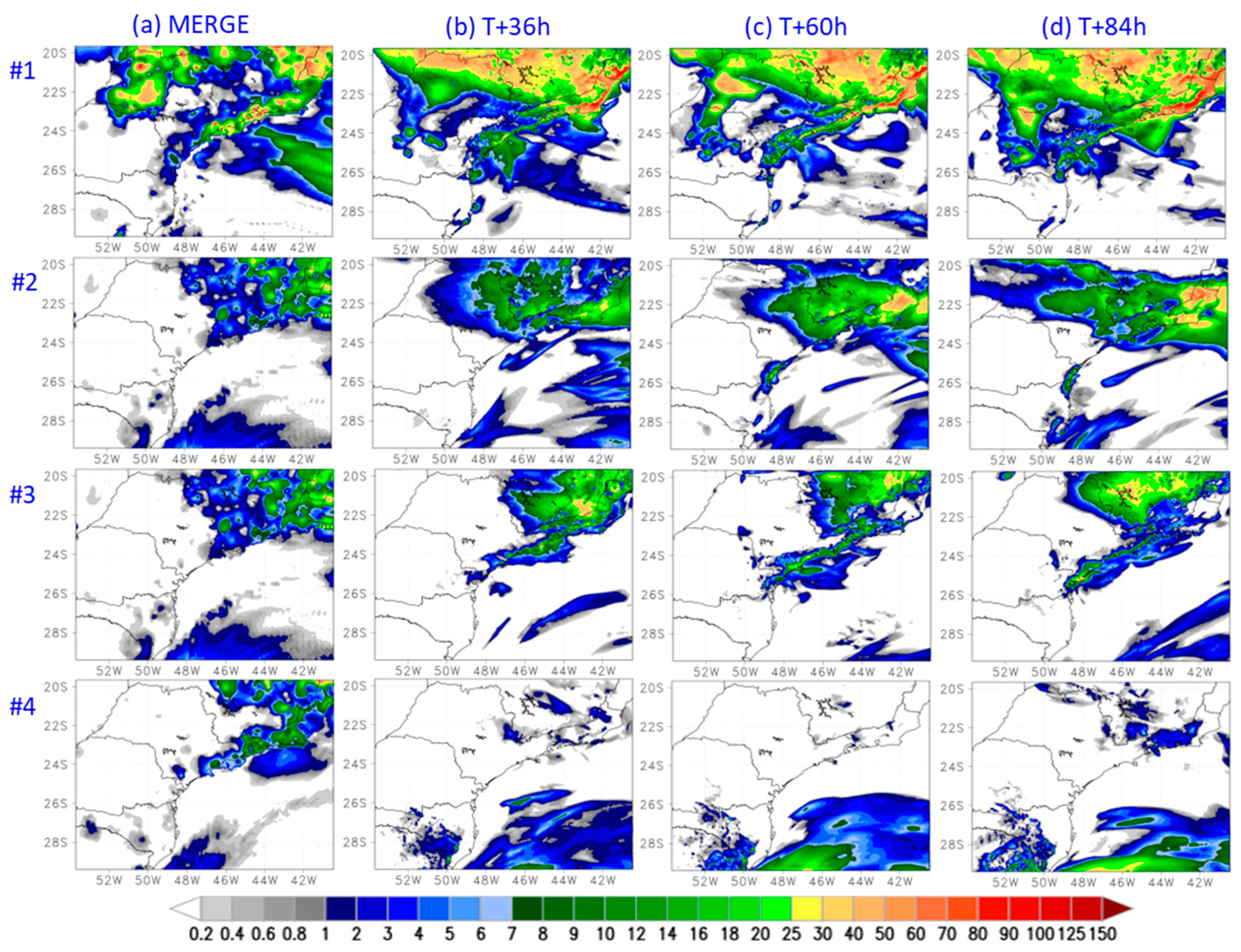
3.2.2. Precipitation Patterns

The storm surge cases were all related to frontal system passages. Here, we assessed the forecast of the precipitation pattern. The precipitation observations used here as a reference were from the daily MERGE dataset [34] produced by the National Institute for Space Research. This dataset resulted from the combination of surface stations and satellite precipitation estimates.

These cases did not exhibit heavy precipitation rates. The forecasts captured the general precipitation patterns (Figure 5).

In case #1, most of the precipitation was observed to the north of the coast of São Paulo, and a small amount was observed along the coast. The forecasts captured this precipitation event, but overestimated the amounts and the area covered by precipitation. In particular, the Eta model produced precipitation forecasts along the coast of São Paulo.

In case #2, the precipitation observed to the north of São Paulo was overestimated by the 60 h and 84 h forecasts. At 36 h, the amounts and the precipitation locations were captured more correctly by the forecasts, but still with some overestimation. In case #3, the precipitation pattern was reasonably forecast, but overestimated, especially along the coast of São Paulo. In case #4, the precipitation band located only in the northern part of the coast was missed by the forecasts at all the lead times. Over the ocean, the forecasts displaced the weather system eastward too fast, leaving just some drizzle around the coast.

In general, the precipitation was well forecast by the system’s Eta-GFS models, but with some overestimation in the total amounts. The driver model provided the displacement speed of the patterns, and the nested high-resolution model provided the details of the pattern.

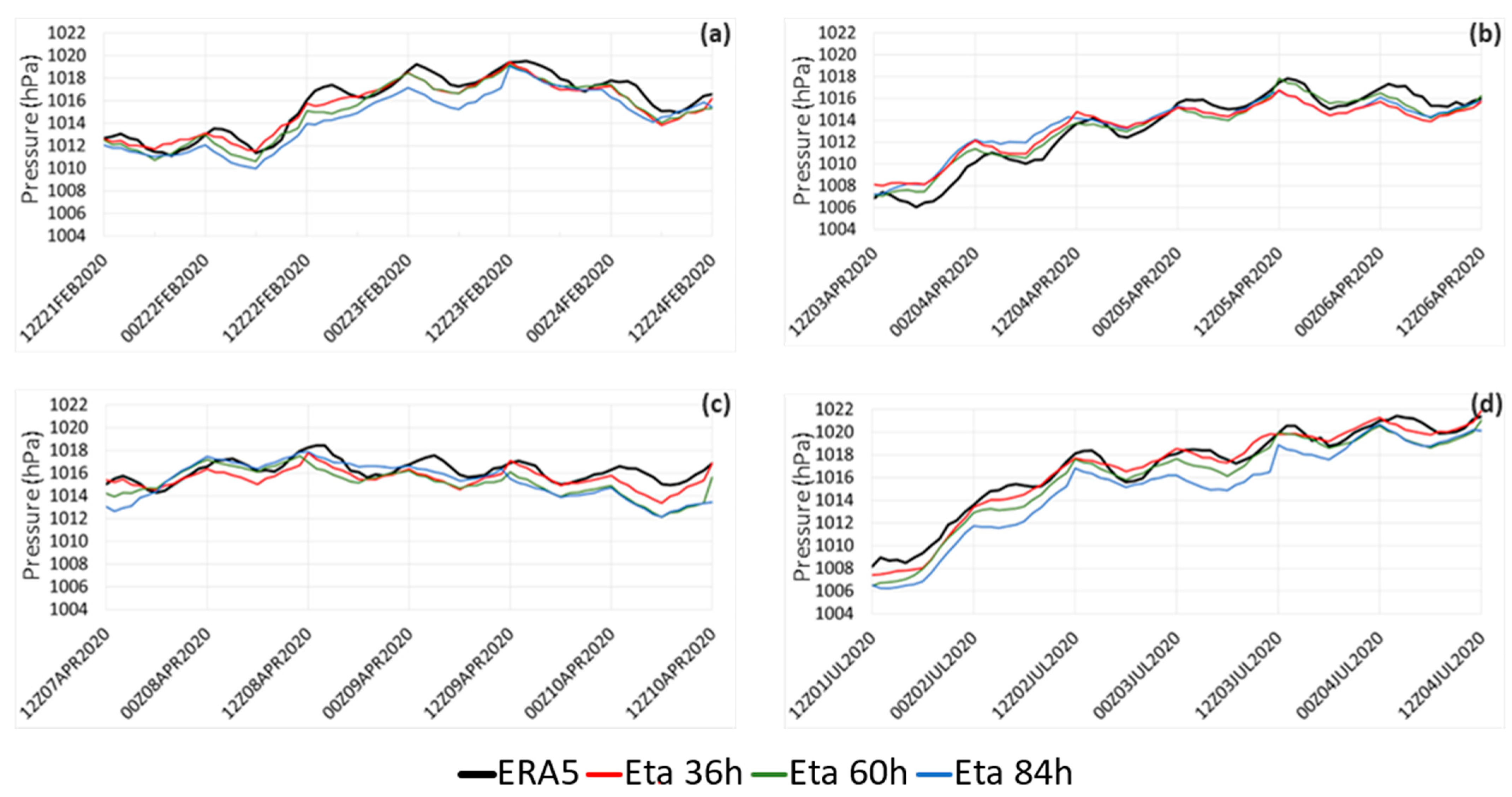
3.3. Offshore Time Series

The time series was taken from a grid box offshore near Santos, at 24° S, 46° W, which is about halfway along the coast. The time series was constructed from the hourly 24 h period that ended in the following forecast lead times: 36 h, 60 h, and 84 h. This assessment should show forecast skill in reproducing the diurnal cycle of the atmospheric pressure and 10 m winds at different forecast lead times during these four storm surge cases.

The forecasts captured the pressure trends in each case period (Figure 6). Except for case #3, all the other cases showed a positive trend, that is, the mean sea-level pressure increasing through the period. This pressure increase was because, when the highest waves reached the coast, the conditions of the western part of the low-pressure system prevailed along the coast of São Paulo. Case #3 showed an almost steady pressure and a slight decrease at the end of the event, which was also captured by the forecasts. The diurnal variability in the mean sea-level pressure was produced by daily radiative heating, which is important near the tropics. The semidiurnal variability followed the tidal cycle, which occurred at 12 h intervals. The diurnal and semidiurnal variations in the pressure were also reproduced; however, the forecasts of these pressure peaks and dips occurred about 2 h in advance of those in ERA5. While the 84 h forecasts tended to underestimate the MSLP, the 36 h forecast curves were generally closer to ERA5. The 84 h and 60 h forecast patterns were very similar.

Figure 7 shows the hourly 10 m winds for the four case studies. In case #1, the 10 m winds strengthened abruptly on 22 February, from 2 m/s at 10Z to 12 m/s at 12Z, and from then on, the winds weakened gradually until 12Z on 23 February. Therefore, during the period of maximum wave heights, the winds along the coast of São Paulo weakened. The wind speed variations during the event were captured by the forecast at different lead times, but the 36 h forecasts were closer to the ERA5 wind speeds. For case #2, the forecasts at the 36 h, 60 h, and 84 h lead times showed larger differences among them. The 36 h forecasts captured the observed variability in the wind speeds closely, while the 84 h forecasts departed largely, particularly around 06Z, 5 February. In case #3, despite the prolonged high wave heights, the wind did not show any peaks, remaining at about 6 m/s during the entire event. The forecasts approximated the observations during the high wave heights.

In general, the observed hourly wind variations during the storm surge events on the coast of São Paulo were followed closely by the forecasts at different lead times. The strong winds on the day immediately prior to a storm and the weakened winds during the storm surges were reproduced by these forecasts.

3.4. Forecast Skill

In order to obtain a quantitative measure of the forecast errors, some evaluation metrics were calculated. These were the mean error (ME) or bias, the root mean squared error (RMSE), and the linear temporal correlation between the forecasts and the validating ERA5 data from the time series (Figure 7). These metrics were applied to the MSLP and 10 m winds, while a categorical evaluation was applied to the precipitation forecasts.

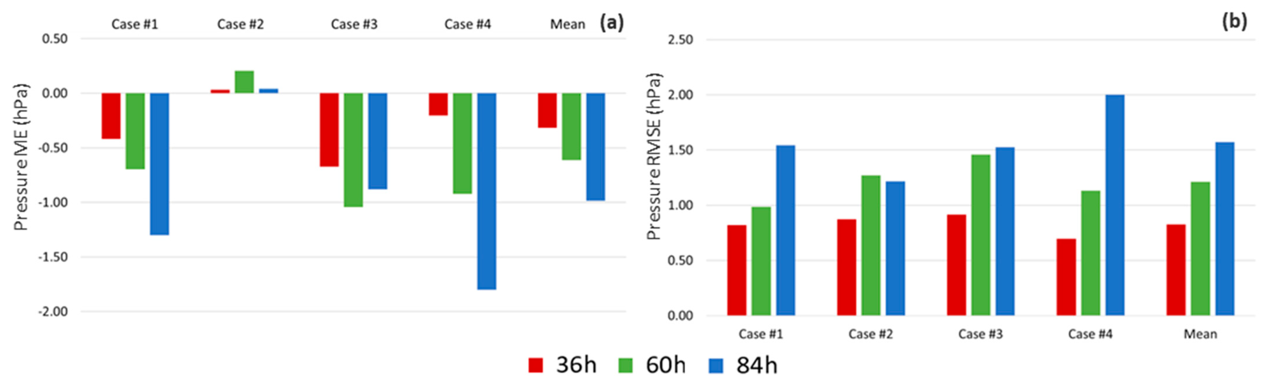
3.4.1. MSLP Evaluation

All cases, except for case #2, showed a systematic underestimate of MSLP (Figure 8). The mean errors in MSLP in the 84 h forecasts were not always the largest, although on average, the mean errors grew from the 36 h toward the 84 h MSLP forecasts. On average, the errors did not exceed |–2.0| hPa. The mean errors for the 36 h forecasts may contain some of the errors of the analyses, since the 36 h forecasts were closer to the initial conditions.

A larger MSLP RMSE was found for the 84 h forecasts of cases #1 and #4, and clearly, the smallest MSLP RMSE was found for the 36 h forecasts in all cases. On average, the RMSE grew steadily from the 36 h to the 84 h forecasts, but these were all below 2.0 hPa.

3.4.2. The 10-m Wind Speed Evaluation

Unlike the MSLP, the mean errors of the wind speeds (Figure 9) were all positive. There were negative and positive errors that compensated for each other during the evaluated three-day period of each event, but, on average, the remaining errors of the 10 m winds were positive, especially for the 60 h forecasts, which was highlighted in the mean for all cases.

The 10 m wind RMSE was the largest for case #4. In this case, the forecast did not capture the short transition from strong to weak winds in the 60 h and 84 h forecasts. On average, the 10 m wind RMSE grew from the 36 h to the 84 h forecasts.

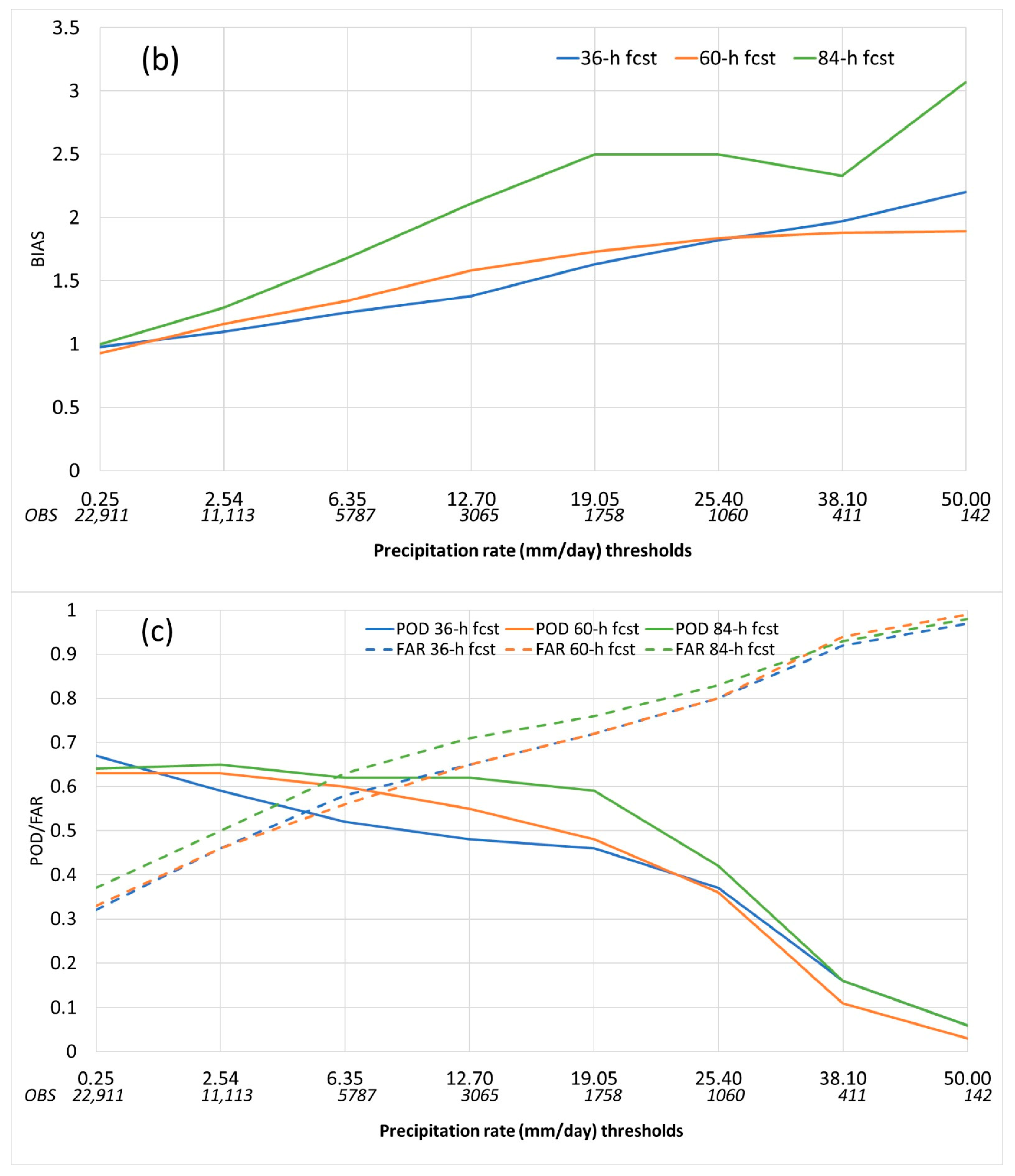
3.4.3. Precipitation Evaluation

The evaluation of the precipitation forecasts was based on a multi-category method, in which each category was an event, and in this case, it was a precipitation rate threshold. A contingency table was produced for each category. Simple scores were applied: the threat score (TS), or critical success index; the bias (BIAS); the probability of detection (POD); and the false alarm rate (FAR), which are defined as follows [35]:

$$TS=\frac{H}{F+O-H}$$

(2)

$$BIAS=\frac{F}{O}$$

(3)

$$POD=\frac{H}{O}$$

(4)

$$FAR=\frac{F-H}{F}$$

(5)

where F is the number of forecast events, H is the number of forecast hit events, and O is the number of observed events in a perfect forecast: TS = 1, BIAS = 1, POD = 1, and FAR = 0.

Eight precipitation thresholds were assessed. The threshold > 0.25 mm/day was used to assess the forecast ability and distinguish between the rain and no-rain events; the thresholds 2.54 and 6.35 targeted the light precipitation rates; the thresholds between 12.7 and 25.4 targeted moderate precipitation rates; and the thresholds 38.1 and 50.0 targeted the heavy and very heavy precipitation rates. The number of observations indicated the uncertainty of the score for each category.

For the four cases, the 24 h accumulated precipitation rates at the forecast lead times of 36 h, 60 h, and 84 h were assessed on the days of maximum wave height (Figure 5).

In terms of distinguishing between rain and no-rain events, the 36 h forecasts had the highest TS (Figure 10a). For the light and moderate precipitation thresholds, the 60 h forecasts scored the highest, and for heavy and very heavy precipitation rates, the 36 h forecasts showed the highest scores again. Although the 84 h forecasts showed similar scores to the other forecast lead times and would indicate useful forecasts, they showed the largest BIAS for most thresholds, which penalized the threat score. The BIAS score showed that for rain/no-rain events, all forecast lead times performed the best (Figure 10b). At all the other thresholds, the forecasts showed biases larger than 1 that increased with increasing thresholds, which indicates that the forecasts overestimated the precipitation.

Due to having the largest BIAS, the 84 h forecasts showed the largest probability of detection scores at all thresholds. On the other hand, the 36 h forecasts, which showed the smallest BIAS, also showed the smallest POD at weak precipitation thresholds. The large biases at all the forecast thresholds also caused a large number of false alarms. The FAR score started low, at around 0.3, for all the forecast lead times of the rain/no-rain events. However, as the precipitation rate thresholds increased, the FAR also increased. The rain/no-rain category had the best performance, with a BIAS and TS of approximately 1 and 0.5, respectively. The performance of this version improved over the 5 km Eta model for southeast Brazil, applied by Calado et al. [36], which underestimated the precipitation, especially at heavy rates. In the study by Calado et al. [36], the Eta model was driven by the CFSR reanalysis, whereas, here, the driver was the GFS forecasts.

4. Discussion

The four selected case studies of storm surges on the coast of São Paulo were produced from low-pressure systems centered around the latitudes 35° S–40° S and 45° W–35° W on the previous day of each coastal storm. This area is east of the preferential cyclogenesis area found by Reboita [37]. The cyclone–anticyclone wave system generally travels over the southeastern part of South America in a northeastward or eastward trajectory. Slowly traveling systems may leave the western part of the cyclone or the eastern part of the anticyclone to blow strong and persistent southerly or southeasterly winds along the coast of South Brazil. These strong winds in an extended area build up waves and result in a storm surge over the open sea that propagates toward the coast of São Paulo.

The cyclonic vortex of case #1 originated farther south, in the area of surface cyclogenesis identified over South America [38]. Some cases had a quasi-explosive-cyclone-like development [39], as the pressure at the low center decreased significantly in 24 h. The cyclonic vortices associated with the low-pressure systems displaced mainly eastward, letting the stronger winds of the western part of the cyclone reach the coast of São Paulo. The storm surge reached the coast on the following day, when the coastal winds had weakened. In these cases, the cyclonic systems had no or minimal westward tilt with height.

The forecasts for these cases started 1.5, 2.5, or 3.5 days before the day that the storm surges reached the coast of São Paulo; therefore, these were 36 h, 60 h, and 84 h forecast lead times. In general, the mean sea-level pressure pattern was well captured by the forecasts; the wind was stronger and closer to the observations for a shorter lead time, but the wind pattern was still reasonably forecast at 84 h. Part of the errors may have been due to the weather systems being slightly ahead or delayed, which was partly due to the GFS forecasts that drove the Eta forecasts through the lateral boundaries.

The model overestimated the 24 h accumulated precipitation, especially in the 84 h forecasts. The BIAS score confirmed the overestimate in the model domain, especially at higher precipitation thresholds, causing a high FAR. The rain/no-rain event was the best-forecast precipitation rate threshold, according to the higher TS, a BIAS closer to 1, and a higher POD. However, at higher precipitation rate thresholds, the TS and POD decreased, and the FAR increased. Overestimating the precipitation forecasts can result in excessive alertness. To reduce this overestimation, the parameters and thresholds of model precipitation production and cloud parameterization schemes should be tuned in the next phase. On the other hand, for an early warning system, precipitation overestimation is an error more acceptable than an underestimation, when dangerous events may be missed.

At a point on the coast, the MSLP increased steadily during the three days of each case, showing the prevailing conditions of the western part of the eastward-propagating cyclone. Hourly forecasts at the point underestimated the MSLP, which was an error that was also noted in most of the model domain. Strong winds generated storm surges, but when the highest waves reached the coast of São Paulo, the local winds became weaker as the pressure increased. The strengthening and weakening of the winds on the coast of São Paulo were reasonably reproduced by the hourly forecasts. The slight underestimation of the mean sea-level pressure, especially around the low-pressure center, increased the horizontal pressure gradient, which increased the wind speed.

The skill for different forecast lead times was strongly dependent on the initial conditions. The scarcity of in situ observations led to initial conditions produced mostly by satellites. The evaluation of high-resolution forecasts also required in situ data. Except for precipitation, this evaluation mostly used the reanalysis from ERA5, despite the much coarser resolution compared to the model forecasts. The Eta model forecasts overestimated the 10 m winds; however, these errors may be smaller as ERA5 tends to underestimate the wind speed in comparison to measurement from in situ data over the ocean around this area [40]. The higher spatial resolution may be suitable to forecast stronger winds in the area. Due to the lack of in situ measurements of significant wave height, the ERA5 wave was used, and this dataset corresponded reasonably well to the news of storm surges at the times of the events.

5. Conclusions

As part of the development of a monitoring and early warning system for storm surges hitting the coast of São Paulo, Brazil, four events of storm surges in 2020 were selected for case studies. The large-scale meteorological features of these cases were analyzed using the ERA5 reanalysis. The Eta model with a 5 km resolution was set up over a domain that covered all of the São Paulo coast to produce short-range forecasts of up to 84 h.

The studied cases indicated a preferential region for forming a low-pressure center over the ocean, at between 35° S–40° S and 35° W–45° W. The deepening of the low pressure was quasi-explosive-cyclone-like. These low pressures did not displace much northward, but rather showed mainly eastward displacements. The region is prone to a low-pressure deepening within about 24 h. At this preferential geographic position, the western half of the low-pressure area blew southeasterly winds at a large extension, producing storm surges in the open sea that reached the São Paulo coast on the following day. By the time the storm surges reached the coast of São Paulo, the local winds were no longer strong. The cold fronts associated with the extratropical cyclones were far away to the north, at about 17° S.

The Eta model forecasts of the mean sea-level pressure showed agreement with the reanalysis, but generally with small underestimates and weaker horizontal gradients. The winds tended to be weaker over the ocean, but near the coast, the wind strength was overestimated on average.

In general, the 36 h forecasts scored best, and the forecast error increased toward the end of the forecasts. The 36 h forecasts were closer to the model’s initial conditions. Forecast error growth is common in weather forecasts, which range from 1 day to about 10 days. These error growths are inherent in model simplifications, discretization, and the equations’ non-linearity. The model’s representation of physics processes, such as turbulent mixing and precipitation production, should be revised to improve the precipitation and wind forecasts. Despite the error growth, the 84 h forecasts were still considered useful for an early warning system or to drive ocean dynamics models for wave forecasting. The use of 84 h forecasts may provide a reasonable outlook on the risks of coming events and enough preparation time to take action and reduce their impacts. However, based on the level of uncertainty in the weather forecasts analyzed in this work, stakeholders should use forecasts with caution. They may deploy resources to mitigate the impacts of the storm surge, but should keep monitoring the forecast updates.

References

1. IBGE. Censo Demográfico 2022; Instituto Brasileiro de Geografia e Estatística (IBGE): Rio de Janeiro, Brazil, 2022. [Google Scholar]
2. Gramcianinov, C.B.; Campos, R.M.; de Camargo, R.; Hodges, K.I.; Guedes Soares, C.; da Silva Dias, P.L. Analysis of Atlantic Extratropical Storm Tracks Characteristics in 41 Years of ERA5 and CFSR/CFSv2 Databases. Ocean. Eng. 2020, 216, 108111. [Google Scholar] [CrossRef]
3. Souza, C.R.d.G.; Souza, A.P.; Harari, J. Long Term Analysis of Meteorological-Oceanographic Extreme Events for the Baixada Santista Region. In Climate Change in Santos Brazil: Projections, Impacts and Adaptation Options; Springer International Publishing: Cham, Switzerland, 2019; pp. 97–134. [Google Scholar]
4. Souza, C.R.G.; Silva, P.L.; Silva, V.D.M. Histórico de Eventos Meteorológicos-Oceanográficos Intensos/Extremos Na Costa de São Paulo (Brasil): 1928–2021. In Proceedings of the XIX Congresso Latino-Americano de Ciências Marinhas—COLACMAR: Panamá City, Panama, 19–23 September 2022; p. 245. [Google Scholar]
5. Sondermann, M.; Chou, S.C.; Souza, C.R.d.G.; Rodrigues, J.; Caprace, J.D. Atmospheric Patterns Favourable to Storm Surge Events on the Coast of São Paulo State, Brazil. Nat. Hazards 2023, 117, 93–111. [Google Scholar] [CrossRef]
6. Sondermann, M.; Chou, S.C.; Tavares, P.; Lyra, A.; Marengo, J.A.; Souza, C.R.d.G. Projections of Changes in Atmospheric Conditions Leading to Storm Surges along the Coast of Santos, Brazil. Climate 2023, 11, 176. [Google Scholar] [CrossRef]
7. Nobre, P.; Siqueira, L.S.P.; de Almeida, R.A.F.; Malagutti, M.; Giarolla, E.; Castelão, G.P.; Bottino, M.J.; Kubota, P.; Figueroa, S.N.; Costa, M.C.; et al. Climate Simulation and Change in the Brazilian Climate Model. J. Clim. 2013, 26, 6716–6732. [Google Scholar] [CrossRef]
8. Chou, S.-C.; Marengo, J.A.; Silva, A.J.; Lyra, A.A.; Tavares, P.; Souza, C.R.G.; Harari, J.; Nunes, L.H.; Greco, R.; Hosokawa, E.K.; et al. Projections of Climate Change in the Coastal Area of Santos. In Climate Change in Santos Brazil: Projections, Impacts and Adaptation Options; Springer International Publishing: Cham, Switzerland, 2019; pp. 59–73. [Google Scholar]
9. Armani, G.; Beserra de Lima, N.G.; Pelizzon Garcia, M.F.; de Lima Carvalho, J. Regional Climate Projections for the State of São Paulo, Brazil, in the 2020–2050 Period. Derbyana 2022, 43, e773. [Google Scholar] [CrossRef]
10. Ruiz, M.S.; Ribeiro, R.B.; Sampaio, A.F.P.; Harari, J.; Chou, S.C.; Chagas, D.J.; Ferreira, R.S.; Marinho, C.; Oliveira, F.; Souza, C.R.G. Previsão Operacional de Ressacas e Inundações Costeiras No Litoral de São Paulo. In Proceedings of the XV Simpósio sobre Ondas, Marés, Engenharia Oceânica e Oceanografia por Satélite, Cabo Frio, Brazil, 27–30 November 2023. [Google Scholar]
11. Ruiz, M.S.; Harari, J.; Ribeiro, R.B.; Sampaio, A.F.P. Numerical Modelling of Storm Tides in the Estuarine System of Santos, São Vicente and Bertioga (SP, Brazil). Reg. Stud. Mar. Sci. 2021, 44, 101791. [Google Scholar] [CrossRef]
12. Ribeiro, R.B.; Sampaio, A.F.P.; Ruiz, M.S.; Leitão, J.C.; Leitão, P.C. First Approach of a Storm Surge Early Warning System for Santos Region. In Climate Change in Santos Brazil: Projections, Impacts and Adaptation Options; Springer International Publishing: Cham, Switzerland, 2019; pp. 135–157. [Google Scholar]
13. Ribeiro, R.B.; Ruiz, M.S.; Sampaio, A.F.P.; Oliveira, F.R.; Santos, A.J.; Borges, J.dM.; Pires, C.P. IARA-BS|Implantação Do Sistema de Alerta Para Ressacas e Alagamentos Na Baixada Santista. In Proceedings of the XXIV Encontro Nacional dos Comitês de Bacias Hidrográficas, Foz do Iguaçu, Brazil, 22–26 December 2022. [Google Scholar]
14. Deltares. Delft3D-FLOW. Simulation of Multi-Dimensional Hydrodynamic Flows and Transport Phenomena, Including Sediments; Deltares: Delft, The Netherlands, 2023. [Google Scholar]
15. Deltares. Delft3D-WAVE. Simulation of Short-Crested Waves with SWAN; Delft Hydraulics: Delft, The Netherlands, 2023. [Google Scholar]
16. Egbert, G.D.; Erofeeva, S.Y. Efficient Inverse Modeling of Barotropic Ocean Tides. J. Atmos. Ocean Technol. 2002, 19, 183–204. [Google Scholar] [CrossRef]
17. Chune, S.L.; Nouel, F.; Fernandez, E.; Derval, C.; Tressol, M. Global Ocean Sea Physical Analysis and Forecasting Products. Product User Manual. Issue 1.5. Copernicus Marine Environment Monitoring Service, 2020. Available online: https://catalogue.marine.copernicus.eu/documents/PUM/CMEMS-GLO-PUM-001-024.pdf (accessed on 24 April 2024).
18. Lin, L.; Demirbilek, Z.; Mase, H.; Yamada, F.; Zheng, J. CMS-Wave: A Nearshore Spectral Wave Processes Model for Coastal Inlets and Navigation Projects; US Army Corps of Engineers Engineer Research and Development Center. Technical Report 8–13, USA, 2008. Available online: https://www.researchgate.net/publication/235088278_CMS-Wave_A_Nearshore_Spectral_Wave_Processes_Model_for_Coastal_Inlets_and_Navigation_Projects (accessed on 24 April 2024).
19. Mesinger, F.; Chou, S.C.; Gomes, J.L.; Jovic, D.; Bastos, P.; Bustamante, J.F.; Lazic, L.; Lyra, A.A.; Morelli, S.; Ristic, I.; et al. An Upgraded Version of the Eta Model. Meteorol. Atmos. Phys. 2012, 116, 63–79. [Google Scholar] [CrossRef]
20. Gomes, J.L.; Chou, S.C.; Mesinger, F.; Lyra, A.A.; Rodrigues, D.C.; Rodriguez, D.A.; Campos, D.A.; Chagas, D.J.; Medeiros, G.S.; Pilotto, I.; et al. Manual Modelo Eta-versão 1.4.2. INPE. São José dos Campos, SP, Brazil, 2023; ISBN 978-65-89159-08-7. Available online: http://urlib.net/8JMKD3MGP3W34T/48G6PU5 (accessed on 24 April 2024).
21. Neumann, B.; Vafeidis, A.T.; Zimmermann, J.; Nicholls, R.J. Future Coastal Population Growth and Exposure to Sea-Level Rise and Coastal Flooding—A Global Assessment. PLoS ONE 2015, 10, e0118571. [Google Scholar] [CrossRef]
22. Hersbach, H.; Bell, B.; Berrisford, P.; Hirahara, S.; Horányi, A.; Muñoz-Sabater, J.; Nicolas, J.; Peubey, C.; Radu, R.; Schepers, D.; et al. The ERA5 Global Reanalysis. Q. J. R. Meteorol. Soc. 2020, 146, 1999–2049. [Google Scholar] [CrossRef]
23. Janjic, Z.I.; Gerrity, J.P.; Nickovic, S. An Alternative Approach to Nonhydrostatic Modeling. Mon. Weather Rev. 2001, 129, 1164–1178. [Google Scholar] [CrossRef]
24. Betts, A.K.; Miller, M.J. A New Convective Adjustment Scheme. Part II: Single Column Tests Using GATE Wave, BOMEX, ATEX and Arctic Air-mass Data Sets. Q. J. R. Meteorol. Soc. 1986, 112, 693–709. [Google Scholar] [CrossRef]
25. Janjić, Z.I. The Step-Mountain Eta Coordinate Model: Further Developments of the Convection, Viscous Sublayer, and Turbulence Closure Schemes. Mon. Weather Rev. 1994, 122, 927–945. [Google Scholar] [CrossRef]
26. Ferrier, B.S.; Jin, Y.; Lin, Y.; Black, T.; Rogers, E.; Dimego, G. Implementation of a New Grid-Scale Cloud and Precipitation Scheme in the NCEP Eta Model. In Proceedings of the 15th Conference on Numerical Weather Prediction; American Meteorological Society: San Antonio, TX, USA, 2022; pp. 280–283. [Google Scholar]
27. Fels, S.B.; Schwarzkopf, M.D. The Simplified Exchange Approximation: A New Method for Radiative Transfer Calculations. J. Atmos. Sci. 1975, 32, 1475–1488. [Google Scholar] [CrossRef]
28. Lacis, A.A.; Hansen, J. A Parameterization for the Absorption of Solar Radiation in the Earth’s Atmosphere. J. Atmos. Sci. 1974, 31, 118–133. [Google Scholar] [CrossRef]
29. Ek, M.B.; Mitchell, K.E.; Lin, Y.; Rogers, E.; Grunmann, P.; Koren, V.; Gayno, G.; Tarpley, J.D. Implementation of Noah Land Surface Model Advances in the National Centers for Environmental Prediction Operational Mesoscale Eta Model. J. Geophys. Res. Atmos. 2003, 108, 2002JD003296. [Google Scholar] [CrossRef]
30. Mellor, G.L.; Yamada, T. A Hierarchy of Turbulence Closure Models for Planetary Boundary Layers. J. Atmos. Sci. 1974, 31, 1791–1806. [Google Scholar] [CrossRef]
31. Paulson, C.A. The Mathematical Representation of Wind Speed and Temperature Profiles in the Unstable Atmospheric Surface Layer. J. Appl. Meteorol. 1970, 9, 857–861. [Google Scholar] [CrossRef]
32. Charnock, H. Wind Stress on a Water Surface. Q. J. R. Meteorol. Soc. 1955, 81, 639–640. [Google Scholar] [CrossRef]
33. National Centers for Environmental Prediction/National Weather Service/NOAA/U.S. Department of Commerce. 2015, Updated Daily. NCEP GFS 0.25 Degree Global Forecast Grids Historical Archive. Research Data Archive at the National Center for Atmospheric Research, Computational and Information Systems Laboratory. Available online: https://rda.ucar.edu/datasets/ds084.1/(accessed on 1 May 2024).
34. Rozante, J.R.; Moreira, D.S.; de Goncalves, L.G.G.; Vila, D.A. Combining TRMM and Surface Observations of Precipitation: Technique and Validation over South America. Weather Forecast. 2010, 25, 885–894. [Google Scholar] [CrossRef]
35. Wilks, D.S. Statistical Methods in Atmospheric Science, 2nd ed.; Academic Press: Cambridge, MA, USA, 2006. [Google Scholar]
36. Calado, R.N.; Dereczynski, C.P.; Chou, S.C.; Sueiro, G.; Oliveira Moura, J.D.d.; da Silva Santos, V.R. Avaliação Do Desempenho Das Simulações Por Conjunto Do Modelo Eta-5 km Para o Caso de Chuva Intensa Na Bacia Do Rio Paraíba Do Sul Em Janeiro de 2000. Rev. Bras. Meteorol. 2018, 33, 83–96. [Google Scholar] [CrossRef]
37. Reboita, M. Ciclones Extratropicais Sobre o Atlântico Sul: Simulação Climática e Experimentos de Sensibilidade. Ph.D. Thesis, University of São Paulo, São Paulo, Brazil, 2008. [Google Scholar]
38. Gan, M.A.; Rao, V.B. Surface Cyclogenesis over South America. Mon. Weather Rev. 1991, 119, 1293–1302. [Google Scholar] [CrossRef]
39. Sanders, F.; Gyakum, J.R. Synoptic-Dynamic Climatology of the “Bomb”. Mon. Weather Rev. 1980, 108, 1589–1606. [Google Scholar] [CrossRef]
40. Cardoso, A.A. Ciclones Subtropicais e Ventos em Superfície no Sudoeste do Oceano Atlântico Sul: Climatologia e Extremos. Ph.D. Thesis, University of São Paulo, São Paulo, Brazil, 2019. [Google Scholar]
Figure 1. Time series of the significant wave heights of the four storm cases that affected the São Paulo coast in 2020. The series is taken for 24.13° S, 45.68° W. The horizontal blue lines indicate the wave height threshold of 2.5 m. The horizontal red lines highlight the periods of the storm surge events when the wave height exceeded 2.5 m.
Jmse 12 00771 g001
Figure 2. Eta model topography (meters) with a 5 km resolution for the area highlighted in red. The curly bracket in black indicates the São Paulo coastal limits.
Jmse 12 00771 g002
Figure 3. The mean sea-level pressure (hPa) and 10 m winds (m/s) (left column); a 500 hPa upward motion (color-shaded) and 500 hPa geopotential height (contours) (Pa/s and meters) (middle column); and 200 hPa streamlines and jet stream (shaded for speed > 35 m/s) (m/s) (right column) on 23 February (case #1, 1st row), 4 April (case #2, 2nd row), 9 April (case #3, 3rd row), and 2 July 2020 (case #4, 4th row), from ERA5. These are the dates around which the maximum significant wave height was observed.
Jmse 12 00771 g003
Figure 4. The mean sea-level pressure (contours every 1 hPa) and 10 m winds (vectors, shading for speeds > 7 m/s). The columns refer to (a) the ERA5 reanalysis and the forecasts at (b) 36 h, (c) 60 h, and (d) 84 h; the rows refer to cases #1 (1st row), #2 (2nd row), #3 (3rd row), and #4 (4th row).
Jmse 12 00771 g004
Figure 5. The 24 h precipitation accumulation (mm/day) at 12Z on the following dates: 23 February (case #1, 1st row), 4 April (case #2, 2nd row), 9 April (case #3, 3rd row), and 2 July 2020. The columns refer to (a) the reanalysis and the forecasts at (b) 36 h, (c) 60 h, and (d) 84 h.
Jmse 12 00771 g005
Figure 6. Time series of the mean sea-level pressure (hPa) taken at 24° S, 46° W for cases #1 (a), #2 (b), #3 (c), and #4 (d), from ERA5 (black curve) and the Eta model forecasts for the following lead times: 12–36 h (red curve), 37–60 h (green curve), and 61–84 h (blue curve).
Jmse 12 00771 g006
Figure 7. Time series of the 10-m wind speed (m/s), taken at 24° S, 46° W for cases #1 (a), #2 (b), #3 (c), and #4 (d), from ERA5 (black curve) and the Eta model forecasts for the following lead times: 12–36 h (red curve), 37–60 h (green curve), and 61–84 h (blue curve).
Jmse 12 00771 g007
Figure 8. The mean error (ME, hPa) (a) and root mean squared error (RMSE, hPa) (b) of the MSLP forecasts at 36 h, 60 h, and 84 h at a grid box over the ocean halfway along the coast of São Paulo.
Jmse 12 00771 g008
Figure 9. The mean error (ME, m/s) (a) and root mean squared error (RMSE, m/s) (b) of the 10 m wind speed forecasts at 36 h, 60 h, and 84 h at a grid box over the ocean halfway along the coast of São Paulo.
Jmse 12 00771 g009
Figure 10. The precipitation threat score (TS) (a), BIAS (b), POD (solid lines) and FAR (dashed lines) (c) for the 36-h, 60-h, and 84-h forecasts. These scores are non-dimensional. The numbers below the x-axis refer to the number of observed events in each precipitation rate threshold.
Jmse 12 00771 g010aJmse 12 00771 g010b