Article

Machine Learning-Based Anomaly Detection on Seawater Temperature Data with Oversampling

1
Vessel Operation & Observation Team, Korea Institute of Ocean Science and Technology, Geoje 53201, Republic of Korea
2
Department of Computer Science & Engineering, Chungnam National University, Daejeon 34134, Republic of Korea
3
Department of Data Science, Ewha Womans University, Seoul 03760, Republic of Korea
*
Authors to whom correspondence should be addressed.
J. Mar. Sci. Eng. 2024, 12(5), 807; https://doi.org/10.3390/jmse12050807
Submission received: 2 April 2024 / Revised: 3 May 2024 / Accepted: 9 May 2024 / Published: 12 May 2024

Abstract

:
This study deals with a method for anomaly detection in seawater temperature data using machine learning methods with oversampling techniques. Data were acquired from 2017 to 2023 using a Conductivity–Temperature–Depth (CTD) system in the Pacific Ocean, Indian Ocean, and Sea of Korea. The seawater temperature data consist of 1414 profiles including 1218 normal and 196 abnormal profiles. This dataset has an imbalance problem in which the amount of abnormal data is insufficient compared to that of normal data. Therefore, we generated abnormal data with oversampling techniques using duplication, uniform random variable, Synthetic Minority Oversampling Technique (SMOTE), and autoencoder (AE) techniques for the balance of data class, and trained Interquartile Range (IQR)-based, one-class support vector machine (OCSVM), and Multi-Layer Perceptron (MLP) models with a balanced dataset for anomaly detection. In the experimental results, the F1 score of the MLP showed the best performance at 0.882 in the combination of learning data, consisting of 30% of the minor data generated by SMOTE. This result is a 71.4%-point improvement over the F1 score of the IQR-based model, which is the baseline of this study, and is 1.3%-point better than the best-performing model among the models without oversampling data.

1. Introduction

Climate change causes a fundamental restructuring of ecosystems and affects human societies and economies. Among the several factors that induce climate change, oceans play an important role in global climate dynamics [1]. Oceans absorb 93% of the heat accumulated in the atmosphere and ocean warming affects most ecosystems [2]. Accurate ocean physical data observations are required to understand the changes in physical properties due to climate change or changes in the marine environment due to natural variability. Ocean physics observations are used for ocean-related climate variability, multilevel climate change, initialization of a coupled climate model of the ocean and atmosphere, and development of ocean analysis or forecasting systems [2].
Representative instruments for observing ocean physics data include the conductivity–temperature–depth (CTD) system, Underway CTD (UCTD), Argo, and mooring buoys [3,4,5,6,7]. Abnormal data may be observed in marine observation equipment due to aging of the equipment, mechanical defects, user errors, and unpredictable problems. It is also observed in rapid changes in the environment corresponding to environmental issues such as hydrothermal diffusion and the inflow of ocean currents [8,9]. Abnormal observational data have negative impacts on marine system modeling and positive impacts on the scientific discovery of environmental and climate change; thus, it is very important to detect anomalies in observational data.
Anomaly detection techniques have been used in a wide range of fields for decades to identify, extract, detect, and remove anomalous components from data. Anomaly detection refers to “the problem of finding patterns in data that do not match expected behavior” [10]. Anomalies can be classified according to the pattern type: global anomalies (point anomalies), contextual anomalies (conditional anomalies), and collective anomalies (group anomalies). Alternatively, they can be classified into local and global anomalies according to the comparison range, and vector anomalies and graph anomalies according to the input data type [11,12,13,14]. Anomalies can be identified using an anomaly detection technique, and the data can be purified by removing the contaminating effect on the dataset.
Anomaly detection methods were performed arbitrarily and passively in the past; however, in modern times, they are performed consistently and automatically using principled and systematic techniques derived from the entire domain of computer science and statistics. Anomaly detection has traditionally been performed using statistical techniques. Statistical anomaly detection techniques detect anomalies in a dataset by assuming that errors or defects are separable from normal data [15,16,17]. Recently, with the advancement in computer system hardware performance, anomaly detection studies have been conducted using data-driven machine learning methods [10,12,13,14]. The machine learning-based anomaly detection method can be performed using a dataset that contains normal and abnormal data with labels or by learning a machine learning model using only the normal dataset. In general, a large amount of training data is required for machine learning-based abnormal data detection methods. However, if the training data are insufficient or the model is trained using excessively high model complexity, the model is likely to be overfitted. Therefore, it is necessary to secure as much training data as possible in terms of modeling; however, there are limitations in securing data for reasons such as cost and inability to reproduce the acquisition environment. To overcome the limitations on the limited resources of these datasets, various studies have been conducted, including techniques to apply weights to a minority class [18,19].
In this study, oversampling-based anomaly detection methods were proposed to overcome the weaknesses caused by the lack of learning data that frequently occurs in existing machine learning-based anomaly detection studies. Oversampling is a technique that creates additional minority class data such that the amount of minority class data is similar to that of the majority class data when the amount of data per class is imbalanced in a dataset [20]. Anomaly detection in seawater temperature data was performed by applying oversampling techniques to seawater temperature data from the CTD system observation data obtained using the research vessel Isabu operated by the Korea Institute of Ocean Science and Technology in the international waters of the Pacific Ocean, the Indian Ocean, and the Sea of the Republic of Korea from 2017 to 2023. The CTD observation system is one of the main instruments for acquiring marine physics data such as pressure, water temperature, and conductivity, which are required for marine science research.
In the CTD seawater temperature observation data, which are vertical profiles by seawater layer, the information of interest was minority anomaly data, which were augmented and used through oversampling to learn the CTD anomaly detection models. As oversampling methods, simple duplication, addition of uniform random variables, Synthetic Minority Oversampling Technique (SMOTE), and autoencoder (AE) techniques have been applied [21,22]. As anomaly detection models, interquartile range (IQR)-based anomaly detection model, one-class support vector machine (OCSVM), and multi-layer perceptron (MLP) models have been used [23,24,25]. The precision, recall, F1 score, and Area Under the Receiver Operating Characteristic Curve (AUROC) were compared as performance evaluation indicators to determine the appropriate ratio of oversampling data and optimal combination of anomaly detection models [26]. CTD observations have been conducted in waters around the world for decades. Actual field observation work that is being carried out is labor-intensive. For this reason, we started the study of data-driven anomaly detection using CTD datasets and machine learning models for automation of observation sites. We hope that the results of this study can be applied to all real sea observation sites. The ultimate goal of this study is to create a universal machine learning model for detecting anomalies in CTD systems. Therefore, the time of acquisition of the observation data, sea area, location, regional characteristics, and relationships were not considered.

2. Related Work

2.1. CTD Error Detection

Studies related to errors in early CTD systems were conducted to minimize the errors that occurred during sensor measurements. Horne and Toole [27] and Gregg and Hess [28] found discrepancies in temperature and conductivity measurements owing to the physical separation of the thermistor and conductive cells and the discrepancy in the response time of the two sensors. Through numerical analysis and experiments, Larson and Pedersen [29] revealed that measuring the temperature of flowing water using thermistors can cause errors because of the heating of the sensor itself owing to viscous effects. Lueck and Picklo [30] developed a method for predicting and correcting the thermal mass effect error, which depends on the speed of passing through a conductivity cell to significantly reduce the salinity error. Ullman and Hebert [31] presented evidence of speed-dependent salinity errors due to thermistor viscosity heating errors when measuring UCTD, and suggested ways to optimize the conductive thermal mass correction required to accurately calculate salinity. Garau et al. [32] proposed a methodology to find correction parameter values that minimize the area between the temperature and salinity curves given by two CTD profiles to correct thermal delay errors in the data, in which CTD sensors without pumps are installed on the glider. Similar to the aforementioned studies, studies related to errors in early CTD were conducted using methods for finding and correcting the causes of errors occurring in the sensor itself.

2.2. Statistics-Based Anomaly Detection

In statistical-based anomaly detection analysis, anomaly data are defined as “an observation considered to be partially or completely out of line with the probability distribution of most data” [15,33,34]. Statistical techniques fit a model to the given data, determine whether new data follow the model through statistical inference, and classify data that are unlikely to have been generated from the model as abnormal based on test statistics. Statistical-based anomaly detection can be divided into (i) parametric, (ii) nonparametric, and (iii) information theory-based methods [35,36,37,38,39].
The parametric technique is based on the null hypothesis, assuming that the data to be tested are generated from the estimated distribution of normal values [40]. The statistics used for the hypothesis test can be considered as abnormal scores [10]. Parametric techniques can be further divided into normal-, regression-, and mixed-model-based methods according to the type of distribution [41,42]. The normal model base assumes that the data are generated from the normal model and uses a Maximum Likelihood Estimator [35]. The distance between each data point and the estimated average value became an abnormal score, and the boundary of the abnormal score was used to determine whether the score was an anomaly. Various methods have been proposed for determining the definition and boundaries of distance, such as the Grubbs’ test, Student’s t-test, Hotelling’s test, and Chi-square test. The regression model basis was applied to the time-series data, and after fitting the regression model of the data, the abnormal score was obtained as the residual between the test data and the regression model. Methods based on regression models include robust regression and Autoregressive Integrated Moving Average models [41,43]. A mixed model base was used by mixing the distribution to be applied to the data. There are methods of applying different distributions to normal and abnormal values and methods of applying mixed distributions only to normal values.
Nonparametric techniques do not assume that the data follow a particular model [44]. Nonparametric techniques have the advantage of being easy to approach realistically because the assumption that data follow a specific distribution is often not established in practice. The observed values of data often use signs or ranks rather than the actual values of random variables. In other words, it is often used when data are more meaningful than observation figures such as signs or ranks. Nonparametric techniques include histogram-and kernel function-based methods. After generating a histogram from the learning data, the histogram-based method determines whether the test observation is normal if it is included in a meaningful section of the histogram; otherwise, it determines that it is abnormal. An abnormal score is calculated based on the frequency of the interval, including the observed value. If the data are multivariate, an anomaly score is obtained from the histogram of each variable and summed to obtain the total anomaly score. Kernel density estimation is a method for estimating a continuous probability density function based on a kernel function and data under the assumption that the data do not follow a specific distribution. Parzen window density estimation is a representative technique [45]. Unlike the Gaussian density estimation method, the kernel density estimation method does not require the average and variance of the data, and the most significant difference is that it determines an appropriate distribution through the given data. De et al. [46] used a histogram-based technique to describe and analyze oceanic magnetic anomaly data. Wei et al. [47] developed a self-adapting vessel traffic behavior recognition algorithm based on multi-attribute trajectory characteristics using Parzen window density estimation.
Information theory-based anomaly detection techniques analyze the amount of information in data using measures such as entropy and relative entropy [48]. Entropy is a term originally used in classical thermodynamics. Entropy is a function of the temperature and refers to the probability that a given amount of heat can be converted into equivalent work. In general, entropy refers to uncertainty. In information theory, the concept of information entropy was introduced to express the possibility of obtaining information by applying the concept of entropy. The central idea of information theory is that unlikely events are more informative than frequently occurring events. Information entropy is a criterion used to classify whether the obtained information is meaningful. Chen et al. [49] used information entropy to extract useful information from the residuals of a predictive model to detect fault conditions in wind turbines. Tang et al. [46] described the minimum differential signal acquired by a pair of magnetic sensors to detect changes in magnetic noise patterns that can detect or locate objects, such as surface ships and submarines. A magnetic anomaly target was detected using an entropy detector. Scully et al. [50] utilized AIS data and information entropy to cluster vessel traffic characteristics.

2.3. Machine Learning-Based Anomaly Detection

Recently, anomaly detection tasks have been performed based on machine learning methods in a wide range of fields. Anomaly detection techniques that use machine learning can be divided into supervised and unsupervised techniques [51]. Research on unsupervised anomaly detection techniques has been actively conducted using various approaches. In the early days of the study, distribution-based anomaly detection techniques [40,52], depth-based anomaly detection techniques [53], and clustering-based anomaly detection techniques [51] have been mainly studied, but recent research trends largely utilize distance- and density-based anomaly detection techniques [54].
Supervised anomaly detection methods require a labeled training set containing both normal and abnormal samples to construct a predictive model. Theoretically, supervised methods have access to more information and provide better detection rates than semi-supervised and unsupervised methods. However, owing to technical problems, supervised anomaly detection methods may not be as accurate as expected. A representative problem is overfitting, owing to the lack of datasets for the machine learning model. In addition, obtaining correct labels for the dataset is challenging, and the training dataset usually contains noise that increases the false alarm rate. Common supervised anomaly detection algorithms include supervised neural networks, support vector machines (SVM), k-nearest neighbors, Bayesian networks, and decision trees [55].
In recent years, along with the explosive interest in artificial intelligence technology, machine learning-based anomaly detection techniques are being studied in various approaches [56,57,58,59,60]. Various industries are studying by applying anomaly detection techniques [61,62,63,64,65,66,67,68,69,70]. In marine engineering, several studies have been conducted to detect anomalies related to ship path movements. Soleimani et al. [71] showed that it is possible to detect a ship moving in an abnormal path using the difference between the actual movement path of the ship recorded by the AIS [72] and the optimal path generated by the A* algorithm [73,74]. Rong et al. [75] simplified a ship’s trajectory using the Douglas and Peucker algorithm [76], extracted turning points, and grouped them using Density-Based Spatial Clustering of Applications with Noise algorithm [77]. Wang et al. [78] presented a new method combining wavelet neural networks and threshold values and combining the two detection strategies to detect anomalies in ocean fixed-point observation time series.

2.4. Class Imbalanced Problem of Anomaly Detection

Class imbalanced data, in which the number of data points per dataset class is imbalanced, can influence that the model may be biased towards predicting the majority class, leading to decreased performance on the minority class [79]. To overcome this problem, undersampling and oversampling techniques have been studied [80]. Undersampling removes majority class samples to balance the data obtained from each class. This method can reduce the training cost of the predictive model; however, the distribution of the majority class may be corrupted, or important data of the majority class can be removed from the dataset. Undersampling methods include random sampling, Tomek links, easy ensembles, balanced cascades, one-sided selection, and MLP-based techniques [81,82,83,84].
In contrast, oversampling generates additional minority class data to generate equal sample frequencies for both classes. Oversampling provides the advantage of properly preserving the distribution of the majority and minority classes but increases the training cost of the predictive model [20]. A typical oversampling technique is the SMOTE technique, which augments minority data. The SMOTE-based method is a key concept in prime number oversampling, a technique for synthesizing new artificial data by interpolating the data of prime numbers instead of duplicating existing data [21]. This technique first uses the k-nearest neighbor algorithm to find the data closest to the data in the minority category and then creates newly synthesized data. In addition, the borderline SMOTE, SMOTEBoost, SMOTE-Tomek, SMOTE-RSB, and adaptive synthetic sampling approach for imbalanced learning (ADASYN) have been developed using the SMOTE technique [85,86,87,88,89,90]. Recently, AE and Generative Adversarial Network (GAN)-based oversampling methods implemented based on natural networks have been studied [91,92].

3. Methodology

3.1. CTD System

The target system of this study was a CTD system, which is a marine instrument that can acquire essential physical data of the ocean for ocean science research, such as conductivity, water temperature, and pressure. In addition, various data, such as dissolved oxygen, pH, turbidity, fluorescence, oil, photosynthetically active radiation, nitrate, and altitude, can be acquired by attaching sensors to the CTD system. CTD systems are used in almost all ocean research vessels owing to their data accuracy, sampling speed, and ease of use. As shown in Figure 1, the CTD system schematic consists of an underwater unit, deck unit, water sampler, winch, winch cable, and operating PC. In this study, a 911plus CTD system was used [93]. The SBE 911plus CTD system can measure sensor data at 24 Hz using eight sensors up to a depth of 10,500 m in marine and freshwater environments. The main housing consists of a communication circuit, pressure sensor, and electronic circuit that collects data. The measurement range of temperature and conductivity is −5 °C to 35 °C and 0 to 7 S/m, the accuracy is ±0.001 °C and ±0.0003 S/m, and the resolution is 0.0002 °C and 0.00004 S/m, respectively. The main causes of errors in the CTD system are poor contact with the underwater connector, watertightness failure, disconnection and shorting of the winch cable, defects in the slip ring, physical damage due to collision with the seafloor, penetration of marine life or foreign matter in the sensor, and user errors. Owing to these unpredictable causes of errors, the CTD system stops running or some observation data are erroneous. In our study, when operating the CTD system, the winch speed was set to 60 m/min according to sea conditions after launch, and data were acquired by descending or ascending to the depth section desired by the user. Owing to the long operation time according to the water depth and fast sampling cycle, the number of acquired data samples was very large, making it difficult to process with the current computer system. Therefore, in this study, the acquired CTD raw observation data were averaged at 1 m depth using the bin average module with SBE data processing software (version 7.26.1.8) and used for CTD anomaly detection.

3.2. Dataset

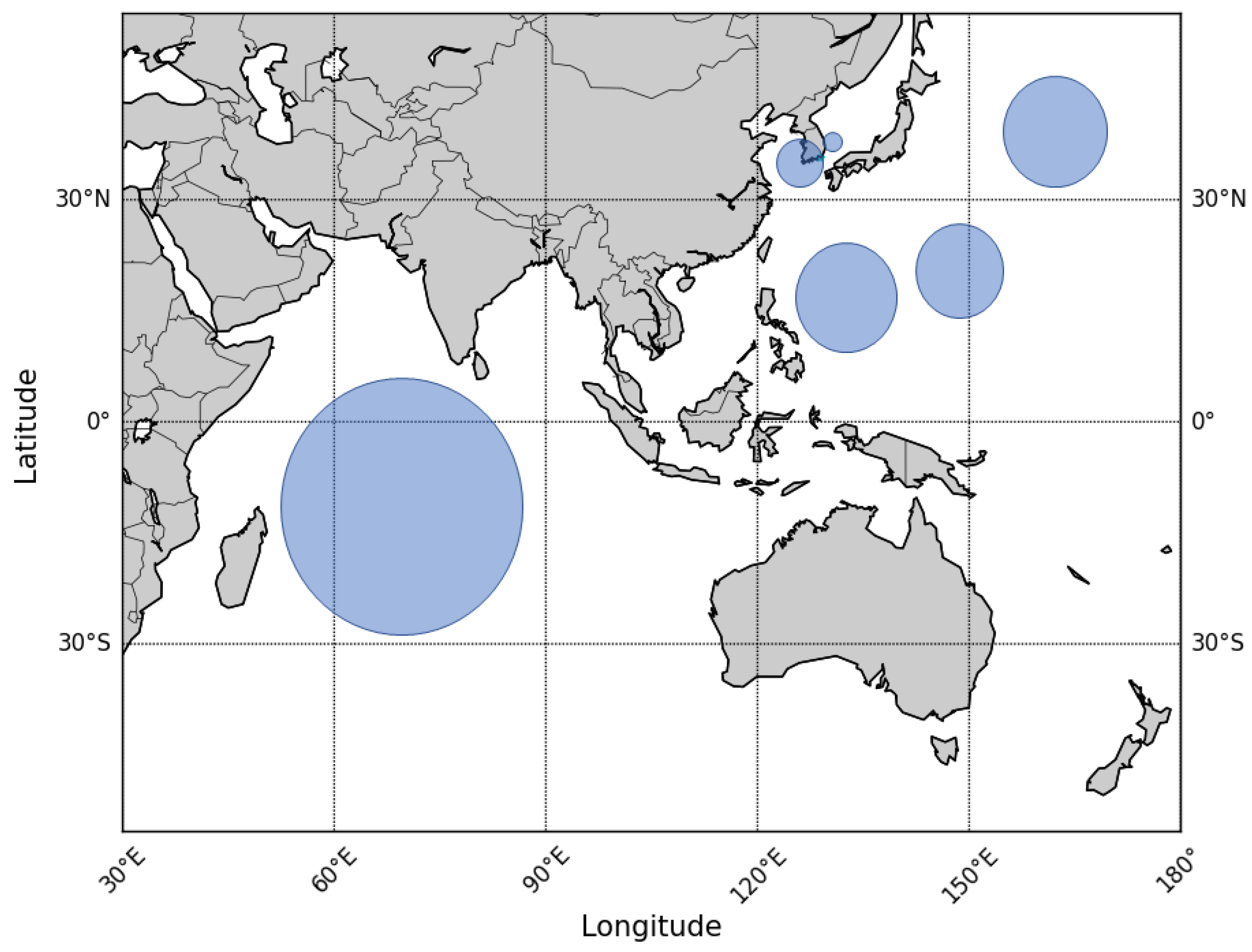
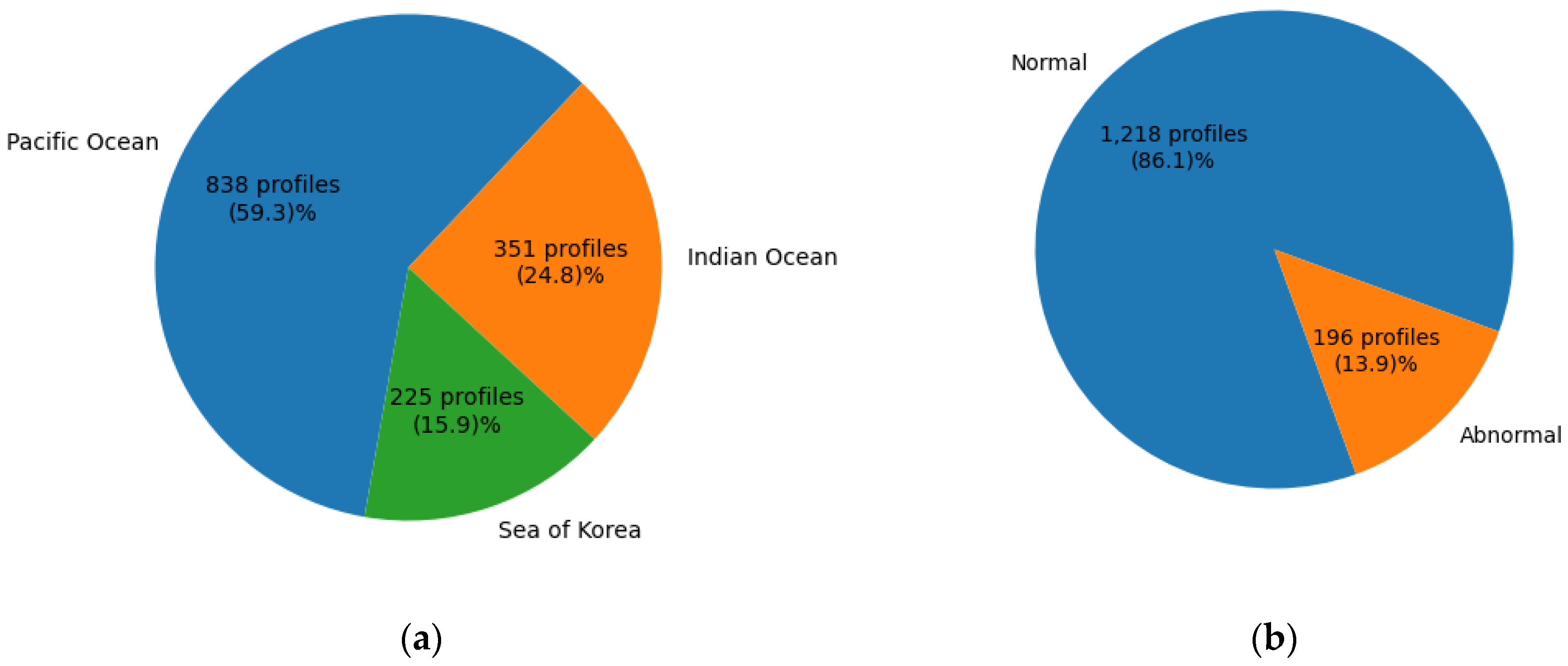
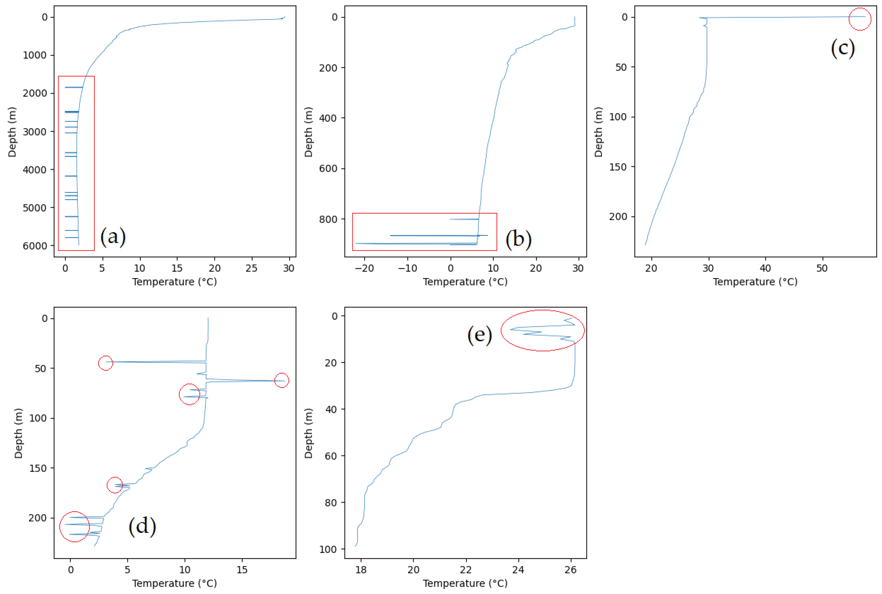
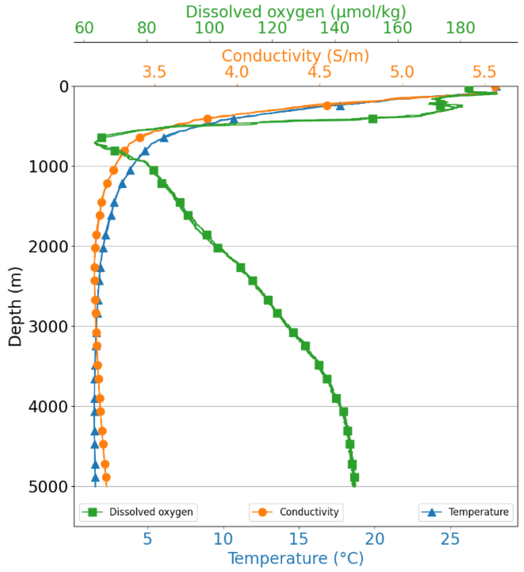
For the machine learning-based anomaly detection study of the CTD system, observational data were created as a dataset. The CTD dataset was acquired through 54 research voyages from June 2017 to April 2023 in the Indian Ocean, Northwest Pacific Ocean, and Korean waters. The location of the CTD data acquisition is shown in Figure 2, where it is marked as areas instead of coordinates, owing to data security issues related to resource exploration. Figure 3 shows the composition ratio of the dataset used in the study by observation area and by normal and abnormal data. The total number of profiles was 1414, consisting of 838 (59.3%) in the Pacific Ocean, 351 (24.8%) in the Indian Ocean, and 225 (15.9%) in the Korean territorial waters. In this study, anomaly detection was performed using only seawater temperature data among the entire CTD dataset. The seawater temperature data create a temperature profile of seawater by seawater layer as part of the CTD dataset. The normal profile and abnormal profile data labeling method involved direct inspection of each individual profile data point by referring to the descriptions in the field notes recorded at the observation site. The criteria for determining normal and abnormal profiles were based on the effective range of the values, the instantaneous rate of change, and empirical knowledge gained from actual field observations. Figure 4 shows the type of anomaly pattern for the CTD seawater temperature profile. Of the total 1414 profiles, 1218 (86.1%) normal and 196 (13.9%) abnormal individual profiles were individually identified and annotated for use as training data in the supervised learning model. Figure 5 shows the obtained CTD observation profile, where the y-axis shows the water depth and the x-axis shows the water temperature, conductivity, and dissolved oxygen.
The CTD acquires data while moving down and up. Therefore, as shown in Figure 5, the observation data were continuously obtained in the upcast and downcast, which is actually one profile, but it looks like two profiles, such as the dissolved oxygen value. When a CTD system is launched, physical damage may occur due to waves and swells on the surface layer. Therefore, instead of raising the CTD sensor parts installed at the bottom of the CTD frame (refer to Figure 1a) to the surface layer, it operates only at the top of the CTD frame at sea level, depending on sea conditions. Therefore, the data acquisition start depth of each profile may be recorded differently depending on the weather conditions at the time of measurement. In addition, the maximum observed depth varied depending on the maximum depth of each sea area and the research purpose.
The dataset structure was created as a three-dimensional arrangement structure with 6000 m (maximum depth) × number of sensor types × acquisition profiles. The dimension of the CTD dataset is 6000 × 8 × 1414. In this study, the dataset structure used is 6000 × 1 × 1414, as only the seawater temperature profile is targeted. The missing values of the section where the actual data did not exist were replaced with a value of zero to represent the unobserved data caused by system failures in the thermocline layer where the seawater temperature changed rapidly. In addition, there are missing sections depending on the purpose of observation and the maximum depth of the sea. Seventy percent of the total dataset was used for CTD anomaly detection model training, and the remaining 30% was used for model testing. Training and testing datasets were used to learn and test the anomaly detection models for the CTD seawater temperature data by dividing the normal and abnormal data into 7:3 ratios.

3.3. Oversampling Methods

Most of the CTD seawater temperature data were normal profiles (1218, 86.1%), and the abnormal profiles (196, 13.9%) with anomalies were a minority. It has imbalanced data problems that can cause performance degradation during machine learning model training. When training a machine learning model with such an imbalanced dataset, it is important to retain the properties of the raw data. The CTD-observed seawater temperature data used in this study have different data acquisition times and locations, so it is necessary to preserve them to learn a machine learning model. Crucially, the number of samples in the dataset is not sufficient compared to the wide range of observed waters. One goal of this study is to minimize type 2 error in statistical hypothesis testing to detect anomalies without omission [94]. In addition, the computational cost may not be considered significant during the initial research stage of model learning. Therefore, we augmented the minority data of the dataset by adopting oversampling methods that can preserve the characteristics of the raw data among the undersampling and oversampling methods that can be applied to the imbalanced data problem.
In this study, the (i) simple duplication, (ii) addition of uniform random variables, (iii) SMOTE, and (iv) AE techniques were used as oversampling methods. The simple duplication method increases the amount of data by simply duplicating the anomalous data, which are already collected from the minority data. The method of adding a uniform random variable involves adding values of 30%, 50%, 75%, and 100% of the uniform random distribution based on the observed value of the majority data to create minority data. The SMOTE method generates data based on the distribution tendency of minority real data. The AE-based oversampling technique generates virtual minority data using reconstruction errors generated during the reconstruction process. In this study, the structure of the AE layer was designed as (6000, 3000, 1000, 1000, and 6000), and minority data were created using the collected minority observation data as input data. In the oversampling process, only 70% of the entire CTD dataset divided into the training dataset was used.

3.4. Anomaly Detection Models

Traditional methods and machine learning-based models that have recently attracted attention have been applied as anomaly detection models. As a traditional method, an IQR-based anomaly detection model was applied, which was adopted as the baseline to evaluate the performance of the anomaly detection methods proposed in this study. The OCSVM and MLP models were applied as machine learning-based anomaly detection models.
The IQR model identifies anomalies statistically [23]. The OCSVM, a method training exclusively on normal data to detect anomalies, was introduced by Schölkopf et al. [95]. Anomalies, which are data points outside the normal range, are identified by establishing a decision boundary. This method is useful when data are not easily divided into groups or when there are few anomalies [96]. The OCSVM methodology is employed for the classification of N-dimensional data sets characterized by a single class, achieved through the delineation of a hyperplane within the data space. Typically, throughout the training phase, a majority dataset is employed. To evaluate the impact of oversampled data on the classification process, we conducted three distinct experimental datasets: one utilizing a solely normal dataset, another with the abnormal dataset, and a third augmented minor dataset by oversampling into the training dataset.
The MLP model is a type of artificial neural network comprising multiple layers of interconnected nodes, structured in a feedforward configuration [97]. Each neuron within the network applies a linear transformation followed by a non-linear activation function to its inputs, enabling the model to capture intricate data patterns. Training of MLPs typically involves backpropagation, where iterative optimization techniques such as gradient descent are utilized to minimize the error between predicted and actual outputs. Due to their capacity to learn complex mappings and flexibility, MLP models are widely employed across various machine learning tasks, including classification, regression, and pattern recognition [98]. The MLP models were created using three models. The first model was designed with 1 hidden layer and 10 hidden units. The second model was designed to have the three hidden layers (10, 15, and 10) of neuronal structures. The third model was designed to have three hidden layers (500, 100, and 10) of neuronal structures. MLP models are designed such that the output value operates as a binary classifier with normal (0) or abnormal (1). For the MLP models and oversampling learning data combination experiments, 20 experiments were conducted for each experimental case to extract the average value of the top 10 model experiments with excellent F1 scores, and the average value was used as an evaluation index for the model.
The training dataset consists of an independent variable, represented by the observed seawater temperature data for each depth, and a dependent variable consisting of a classification value that labels whether or not an anomaly is present. For training and testing the anomaly detection model, 1414 CTD data were divided into 70% (989) model training data and 30% (425) model test data. The training and test data were equal to the ratio of normal-to-abnormal data for the entire dataset. Consistent division into training and test datasets was employed across all experimental cases. The training and test data comprised 852 and 137 normal and 366 and 59 abnormal profiles, respectively. We augmented the training dataset using the proposed oversampling techniques with 366 abnormal profiles included in the training dataset, classified as anomalies.
When modeling the IQR-based anomaly classifier, the entire water depth interval (6000 m) for 989 training data profiles was used, and the lower quartile (Q1: first quartile) and upper quartile (Q3: third quartile) were calculated for each water depth per meter. In the model test experiment, the anomaly detection performance was evaluated up to the maximum observed water depth for 425 test data points. If the seawater temperature data crossed the boundary of Q1 at more than five points, they were classified as anomalies. The OCSVM model was trained using a normal profile, which comprised the majority data, and an abnormal profile, which comprised the minority data, among the measured training data. In addition, when training a model with oversampled data, the minority data were used at 30%, 50%, 75%, and 100% ratios compared to the majority data. The MLP models were trained by applying the actual measured learning data and minority data generated by oversampling at rates of 30%, 50%, 75%, and 100% compared to the majority data. The MLPs were designed to perform binary classification by labeling the anomalous information of the CTD observation profile with binary values, such as normal (0) or abnormal (1), for supervised learning.

4. Experiments and Evaluation

4.1. Performance Metrics

Evaluation of the results is an important process in machine learning procedures. Various approaches can be used, ranging from qualitative assessments based on expertise to quantitative accuracy assessments based on sampling strategies. Because the environmental settings and datasets used in practice are different, no algorithm can satisfy all requirements and cannot be applied to all studies [99]. For example, classification accuracy is limited when evaluating classifiers in applications with class-imbalance problems. Therefore, depending the purpose, the sensitivity (recall), specificity, F1 score, precision, and accuracy can be used as indicators for evaluating the performance of binary classifiers. These evaluation indicators were calculated using true positives, false positives, true negatives, and false negatives, as shown in Equations (1)–(5), based on the confusion matrix in Table 1. Generally, sensitivity, specificity, and the receiver operating curve (ROC) are used together when the number of true and false sets is similar and true negatives can be accurately identified. Sensitivity, precision, and accuracy were combined and used together, and false sets are used for ambiguous cases. Depending on the situation, all evaluation indicators can be used in full.
S e n s i t i v i t y = T P T P + F N
S p e c i f i c i t y = T N T N + F P
P r e c i s i o n = T P T P + F P
A c c u r a c y = T P + T N T P + T N + F P + F N
F 1   s c o r e = 2 × P r e c i s i o n × S e n s i t i v i t y P r e c i s i o n + S e n s i t i v i t y
Sensitivity is the rate of true prediction when entering the true set. Specificity measures the ability of a model to identify true negatives among all actual negatives correctly. Precision is the percentage of correct answers among those predicted by a classifier. The accuracy is calculated using sensitivity and specificity. Also, accuracy represents the classification rate for the entire dataset. Accuracy cannot be used as a performance indicator when the detection of the minority dataset in the classification problem is important. Therefore, performance evaluation indicators must be appropriately determined according to the purpose.
Sensitivity refers to the correct classification rate of positive data among all actual positive data. It tends to increase as the positive prediction rate increases; however, other metrics, such as precision and specificity, may decrease. Therefore, other evaluation indicators are needed to compensate for these limitations. The F1 score is a harmonized average of precision and sensitivity, which evaluates how well the model predicts the positive class in terms of precision and sensitivity. It can be used as a balanced evaluation indicator without any drawbacks to anomaly detection with class imbalanced data.
The ROC plots the relationship between sensitivity and specificity at all possible thresholds for a binary classification model. This describes the performance of a binary classifier system with a change in the classification threshold. In other words, the ROC is a graph representing the ratio of true positives to false negatives when the decision threshold is changed. The AUROC numerically computes the model’s identification performance using the area under curve (AUC) of the ROC, providing quantified evaluation scores on how successfully and accurately the model separated the positive and negative observations. A classifier model with an AUROC value of 0.5 or less is classified as a random classifier, indicating that the classification result is meaningless [26].
The most important performance in the anomaly detection of CTD seawater temperature data with class-imbalanced data problems is to increase sensitivity so that anomalies in the observation data are not missed. However, the disadvantage of largely emphasizing only the sensitivity, which is a performance evaluation index, is that the model can focus only on accurately identifying the positive class, ignoring information related to accuracy. Therefore, it is difficult to accurately evaluate the overall performance of the model, and it is important to consider the performance in various aspects in practical applications. The F1 score is calculated as the value of precision and sensitivity as a performance evaluation index to overcome the aforementioned problems. For this reason, in this study, we adopted the F1 score as the main indicator for evaluating the proposed experimental case based on our problems.

4.2. Experimental Setting

The specifications of the computer system we used in this study consist of CPU: Intel(R) Core(TM) i7-6700K CPU @ 4.00GHz, RAM: 64 GB, GUP: NVIDIA GeForce GTX 1070, SSD: Samsung 850 PRO 1 TB. The programming code was implemented with the Python, and the main libraries used were imblearn.over_sampling.SMOTE. The Dense and Activation modules of tensorflow.keras were used to implement AE oversampling. sklearn.sm.OneClassSVM and sklearn.neural_network.MLPClassifier modules were used for the anomaly detection model. For the performance evaluation of the model, the rock_curve, rock_auc_score, and confusion_matrix of sklearn.metrics were used. In addition, sklearn.preprocessing.MinMaxScaler and sklearn.model_selection.train_test_split modules were used to handle the dataset. Models and functions not mentioned were directly implemented.
The SVM model was implemented with default hyperparameters in the library. The hidden layers (hidden_layer_sizes) of the MLP models were set to MLP-1 (10), MLP-2 (10, 15, 10), and MLP-3 (500, 100, 10). The maximum number of iterations (max_iter) was set to 500. The activity function relu was used for the hidden layers of MLP models. The remaining unmentioned hyperparameters used default values provided by the library.

4.3. Experimental Results

In this study, the F1 score was adopted as the representative indicator to evaluate the anomaly detection model. The results of the seven models with the best F1 score performance among the performance experiments on anomaly detection of CTD seawater temperature observation data are summarized in Table 2, along with the IQR model results adopted by the baseline of this study, and the comparative performance can be confirmed in Figure 6. The results of the entire combination experiment, including these seven models, are presented in the tables and figures in the Appendix. Each model was named in the following order [anomaly detection model-oversampling method-oversampling data ratio]. Here, the oversampling data ratio is the ratio of the primary data, including the oversampling data, to the majority data of the training data set. This experiment used the oversampling data ratio of 30%, 50%, 75%, and 100% compared to the majority data. In the case of the random uniform variable addition method, a random uniform distribution rate was added to the observed value instead of the oversampling data ratio. Additionally, the last character “S” in the model name string is a scale flag. If there is a character S, it is using the scaled dataset.
First, Figure 6a shows the graph of the F1 score values of the IQR model and the top-7 machine learning model. In the result, machine learning-based anomaly detection models outperformed a traditional statistical method IQR. The performance of MLP-2-S-30 (0.882) resulted in a 71.4%-point improvement in the F1 score compared to the IQR model (0.168) as the baseline for performance evaluation in this study. This result shows that our approach is appropriate for anomaly detection of CTD seawater temperature profiles applying machine learning models.
Figure 6b shows a comparison of F1 score values of the top seven machine learning models. As shown in Table 2, the model with the best F1 score among all the experimental results was MLP-2-S-30 (0.882). In addition, the MLP-2-S-30 model improved the F1 score by 1.3%-point compared with MLP-1 (0.869), which was the best model among the experimental results without applying oversampling data. Furthermore, the MLP-2-S-30 experimental case has a lower standard deviation and higher AUROC than the MLP-1 experimental case in Table 2. This result can be one piece of evidence that the performance improvement of the MLP-2-S-30 experimental case is valid. In terms of AUROC, the MLP-2-A-50 experimental case (0.914) and MLP-2-S-50 experimental case (0.914) showed maximum performance. However, we aim to minimize type 2 error in our problem. Therefore, the MLP-2-S-30 experimental case with the highest F1 score value is evaluated as the optimal case. Based on the results of this experiment, the possibility of an anomaly detection method for CTD observation data using a machine learning model was confirmed, and the performance of the CTD anomaly detection machine learning model could be improved through the oversampling of minority data using limited observation data.
Table 3 compares the generalization performance of each CTD anomaly detection model. Rows #1 to #9 are models using plain training data without oversampling data, and rows #10 to #19 are the results of calculating the average value for each model according to the scale and oversampling methods. In terms of the generalization performance evaluation, results that satisfied expectations were not derived. In the case of the MLP-1 model (#4, 0.869), the F1 score showed at least 9.9%-point better performance than the average value of the MLP model (#14, 0.77) with oversampling. The oversampling-based CTD anomaly detection methods proposed in this study did not show superior performance in terms of generalization performance compared with the experimental case (#4) using plain learning data. In addition, in the case of OCSVMs, the maximum value of AUROC performance was 0.504 (refer to Table A1); in most oversampling combination experiments, it was confirmed that the model was not suitable for detecting CTD seawater temperature data anomalies, as it was less than 0.5. In rows #4–#9, #14, and #15, the experimental cases without scale performed better than the experimental cases with scale. Therefore, we concluded in our problem that it is better to utilize the training dataset without scale. In the results of rows #11–#14 of Table 3, the MLP-2 model is evaluated as a model suitable for our problem with the best F1 score performance among all MLP models. In the results of rows #16–#19 of Table 3, it was confirmed that the duplication oversampling technique showed the best F1 score in the overall oversampling technique; however, the standard deviation has increased significantly compared to other techniques. For this reason, we evaluate that SMOTE or AE-based oversampling techniques are appropriate. Based on the generalization performance evaluation, we reached one conclusion that it is appropriate to perform anomaly detection of the CTD seawater temperature profile by applying the MLP-2 model, scale not applied, SMOTE, or AE-based oversampling. Through the results of this study, we confirmed the need for ablation research through a generalization performance comparison of the results of several machine learning models and oversampling data combination experiments.

5. Conclusions

We performed an anomaly detection study on a seawater temperature dataset of CTD observation profiles. The main contribution of this study was to discover a model in which the proposed machine learning model can detect abnormal profiles better than a traditional statistical technique in the seawater temperature dataset. Furthermore, we showed that the anomaly detection performance of machine learning models can be improved by increasing the training dataset with the oversampling technique. Extensive experiments were conducted to show that our proposed approach was available and excellent in performance. In addition, the proposed experimental case was analyzed using performance evaluation indicators suitable for the anomaly detection problem of the seawater temperature dataset. Our research methods and results can be applied to automation studies of ocean observations to acquire of essential marine physical data.
As subsequent studies, we plan to continue to secure CTD observation data for verifying generalization performance by using independent datasets and use various machine learning models, oversampling methods, and dimensionality reduction methods to expand or ablate research, and anomaly detection studies of all available sensor data will be performed. In addition, we plan to expand the real-time anomaly detection research of CTD systems when exploring real sea areas and ultimately conduct a series of studies on the development of unmanned technology for marine research vessel observations.

Author Contributions

Conceptualization, H.K. and D.K.; data curation, H.K.; formal analysis, S.L.; methodology, H.K., D.K. and S.L.; resources, H.K.; software, H.K.; supervision, D.K. and S.L.; validation, H.K.; visualization, H.K.; writing—original draft preparation, H.K.; writing—review and editing, D.K. and S.L. All authors have read and agreed to the published version of the manuscript.

Funding

This research was supported by Korea Institute of Marine Science & Technology Promotion (KIMST) funded by the Ministry of Oceans and Fisheries Korea, grant number 20170411, 20190033, 20210634, 20210696, 20220509, 20220548, and 20220566. This research was also funded by the KIOST projects, grant number PEA0111, BSPE99771-12262-3, and PO01490. This research was also supported by Institute of Information & communications Technology Planning & Evaluation (IITP) grant funded by the Korea government (MSIT) (No.RS-2022-00155857, Artificial Intelligence Convergence Innovation Human Resources Development (Chungnam National University) and No. RS-2022-00155966, Artificial Intelligence Convergence Innovation Human Resources Development (Ewha Womans University)).

Institutional Review Board Statement

Not applicable.

Informed Consent Statement

Not applicable.

Data Availability Statement

The data are not publicly available due to scientific needs.

Acknowledgments

The authors would like to thank Dong-Han Choi, Kiseong Hyeong, Jimin Lee, Dong-Jin Kang, Jung-Hoon Kang, Sok Kuh Kang, Dongsung Kim, Intae Kim, Jonguk Kim, Suk Hyun Kim, Sung Kim, Young-Tak Ko, Jae Hak Lee, Hong Sik Min, Young-Gyu Park, Kongtae Ra, Taekeun Rho, Chang-Woong Shin, Seung-Kyu Son, and Jae-Hun Park for providing us with the raw CTD data. We also thank Dug-Jin Kim, Saehun Baeg, Dong Jin Ham, Sang-Do Heo, Hwimin Jang, Changheon Jeong, Wooyoung Jeong, Daeyeon Kim, Young-June Kim, Gyeong-mok Lee, Gun-Tae Park, and RV Isabu crews for acquiring CTD data on the rolling deck on the oceans.

Conflicts of Interest

The authors declare no conflicts of interest.

Appendix A

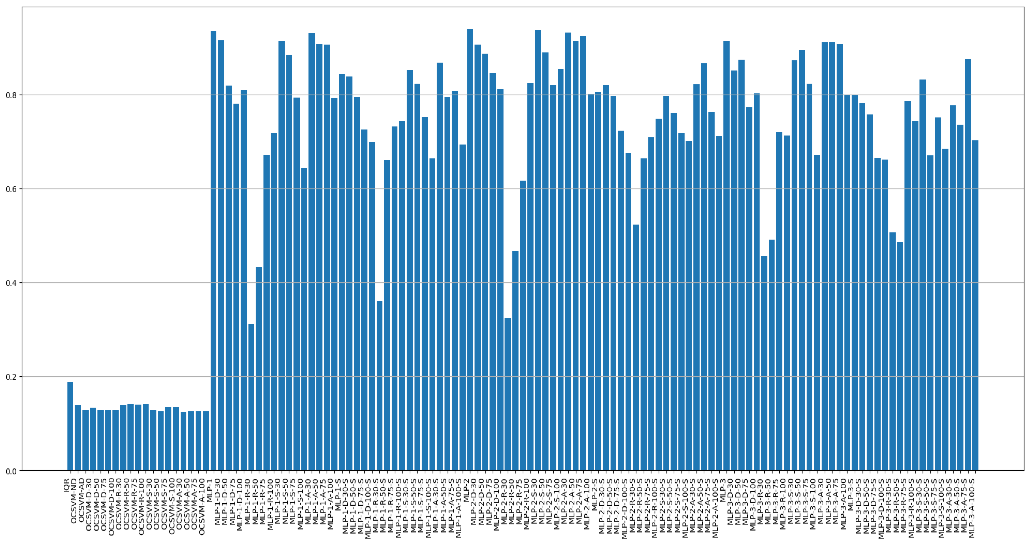
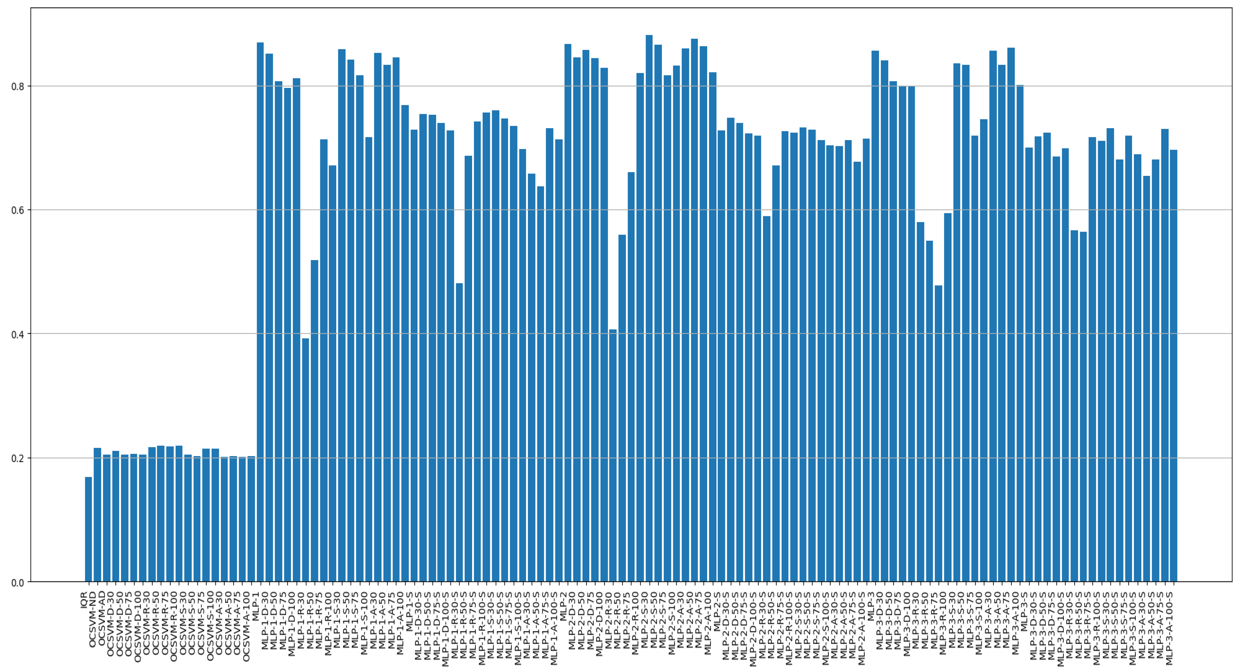
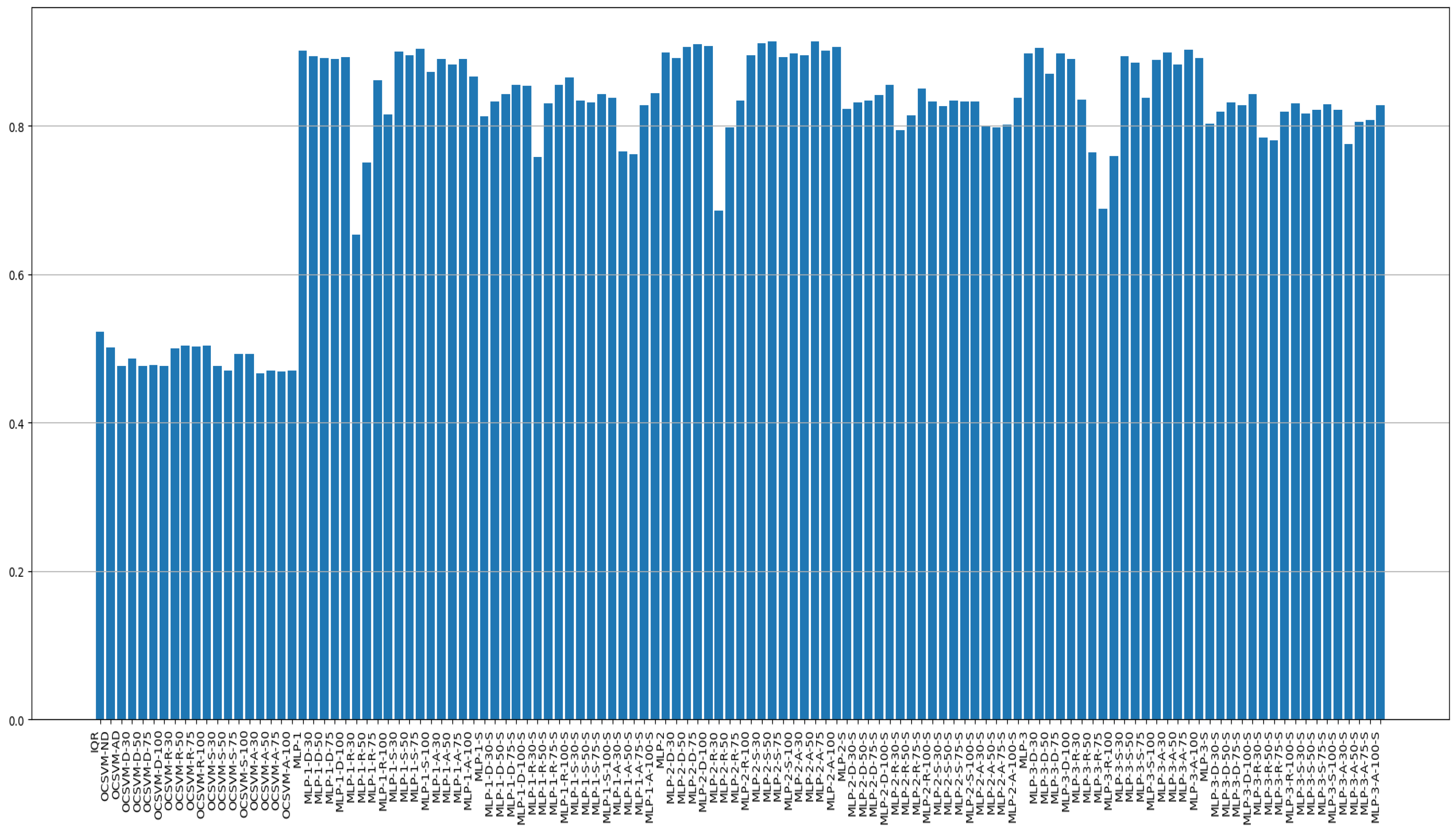
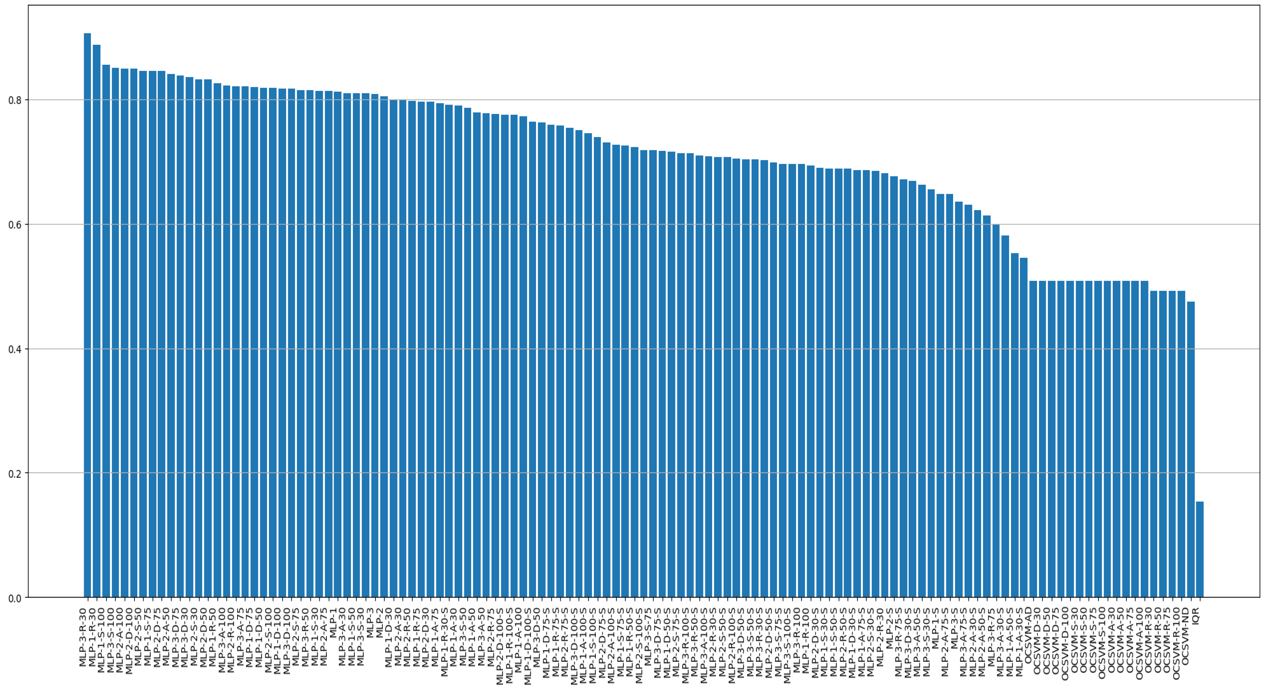
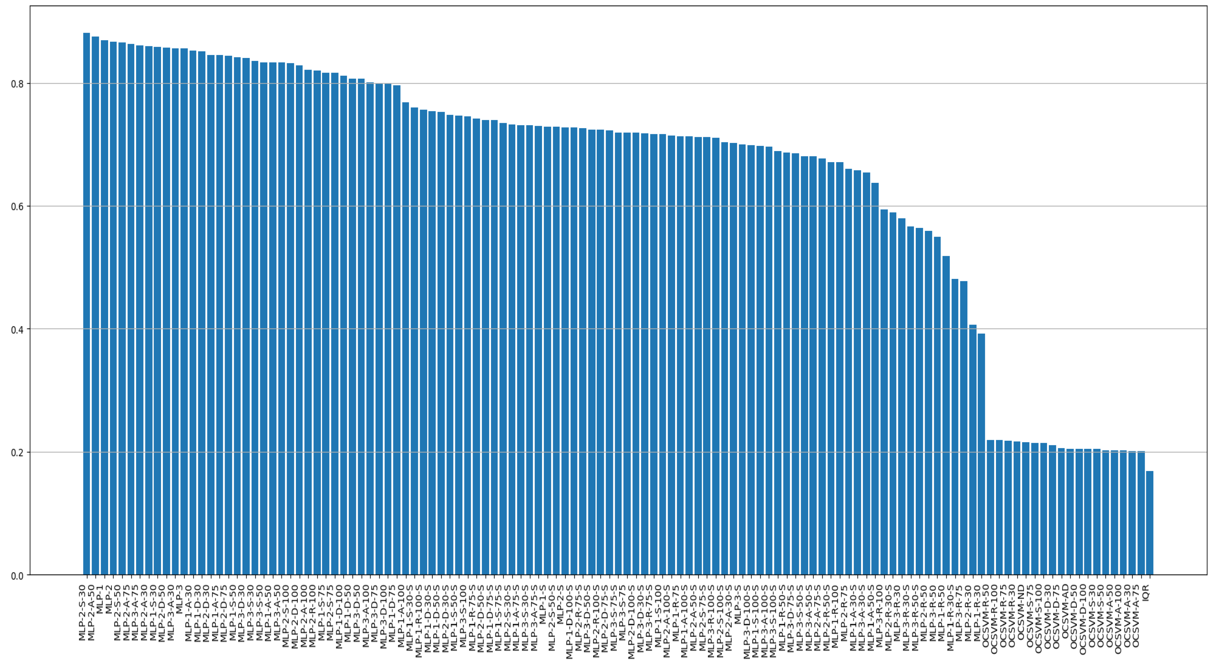
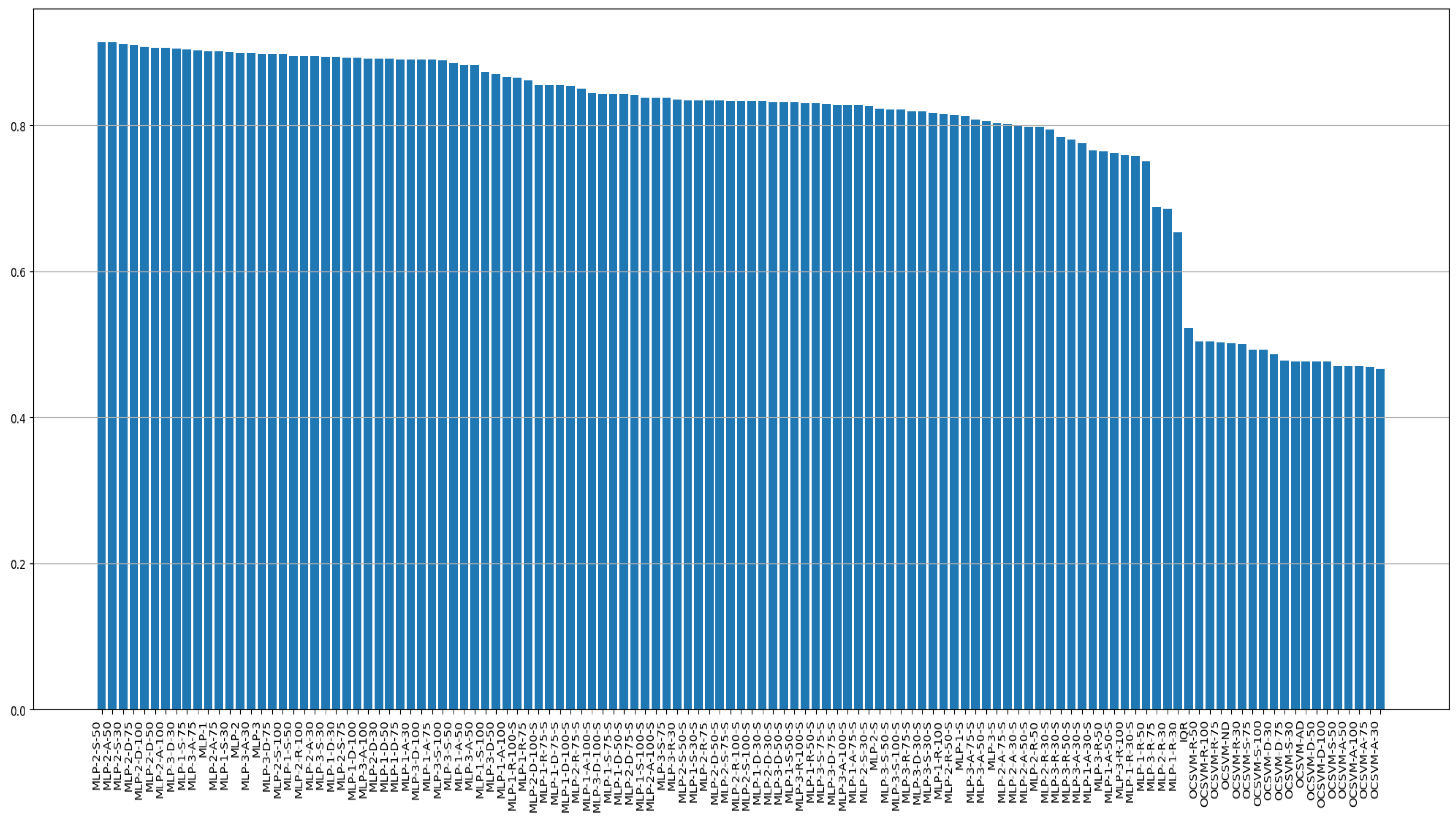
Table A1 shows the overall results of 121 combination experiments on anomaly detection of CTD seawater temperature observation data performed in this study. OCSVM-ND is an experimental result learned using only normal data, and OCSVM-AD is a result learned using only abnormal data. Figure A1, Figure A2, Figure A3 and Figure A4 shows sensitivity, precision, F1 score, and AUROC listed in the order of model names in Table A1, and Figure A5, Figure A6, Figure A7 and Figure A8 shows the indicators of sensitivity, precision, F1 score, and AUROC in order of highest.
Table A1. Performance evaluation of all cases for anomaly detection of the CTD seawater temperature data.
Classification ModelDatasetScore
Model TypeModel NameScale (0–1)Oversampling
(Augmentation)
Sensitivity
(Recall)
PrecisionF1 Score (Std.)AUROC (Std.)
Traditional methodIQRxx0.1530.1880.1680.523
OCSVMOCSVM-ND
(normal data)
xx0.4750.1390.2150.501
OCSVM-AD
(abnormal data)
xx0.5080.1280.2050.476
OCSVM-D-30xDuplication 30%0.5080.1330.2110.486
OCSVM-D-50xDuplication 50%0.5080.1280.2050.476
OCSVM-D-75xDuplication 75%0.5080.1290.2060.478
OCSVM-D-100xDuplication 100%0.5080.1280.2050.476
OCSVM-R-30xUniform random 30%0.4920.1390.2160.5
OCSVM-R-50xUniform random 50%0.4920.1410.2190.504
OCSVM-R-75xUniform random 75%0.4920.140.2180.503
OCSVM-R-100xUniform random 100%0.4920.1410.2190.504
OCSVM-S-30xSMOTE 30%0.5080.1290.2050.477
OCSVM-S-50xSMOTE 50%0.5080.1260.2020.47
OCSVM-S-75xSMOTE 75%0.5080.1350.2140.492
OCSVM-S-100xSMOTE 100%0.5080.1350.2140.492
OCSVM-A-30xAE 30%0.5080.1250.2010.467
OCSVM-A-50xAE 50%0.5080.1260.2020.47
OCSVM-A-75xAE 75%0.5080.1260.2010.469
OCSVM-A-100xAE 100%0.5080.1260.2020.47
MLP-1
hidden layer sizes
(10)
MLP-1xx0.8120.9360.869 (0.021)0.901 (0.015)
MLP-1-D-30xDuplication 30%0.80.9150.852 (0.023)0.894 (0.023)
MLP-1-D-50xDuplication 50%0.8190.8190.807 (0.062)0.891 (0.022)
MLP-1-D-75xDuplication 75%0.820.7810.796 (0.041)0.891 (0.03)
MLP-1-D-100xDuplication 100%0.8170.810.811 (0.035)0.892 (0.014)
MLP-1-R-30xUniform random 30%0.8880.3120.392 (0.172)0.654 (0.145)
MLP-1-R-50xUniform random 50%0.8260.4330.519 (0.197)0.751 (0.116)
MLP-1-R-75xUniform random 75%0.7970.6720.713 (0.081)0.862 (0.052)
MLP-1-R-100xUniform random 100%0.6930.7180.671 (0.115)0.816 (0.073)
MLP-1-S-30xSMOTE 30%0.8140.9140.858 (0.021)0.9 (0.025)
MLP-1-S-50xSMOTE 50%0.810.8850.842 (0.02)0.896 (0.023)
MLP-1-S-75xSMOTE 75%0.8460.7930.816 (0.023)0.904 (0.013)
MLP-1-S-100xSMOTE 100%0.8560.6440.717 (0.147)0.873 (0.071)
MLP-1-A-30xAE 30%0.790.9310.852 (0.032)0.89 (0.032)
MLP-1-A-50xAE 50%0.780.9070.833 (0.047)0.882 (0.036)
MLP-1-A-75xAE 75%0.7930.9070.845 (0.022)0.89 (0.019)
MLP-1-A-100xAE 100%0.7730.7930.769 (0.034)0.867 (0.042)
MLP-1-Sox0.6470.8440.729 (0.029)0.813 (0.025)
MLP-1-D-30-SoDuplication 30%0.6870.8390.754 (0.016)0.832 (0.01)
MLP-1-D-50-SoDuplication 50%0.7150.7950.752 (0.021)0.842 (0.01)
MLP-1-D-75-SoDuplication 75%0.760.7250.739 (0.018)0.856 (0.016)
MLP-1-D-100-SoDuplication 100%0.7650.6980.727 (0.031)0.855 (0.011)
MLP-1-R-30-SoUniform random 30%0.7920.3610.481 (0.103)0.759 (0.07)
MLP-1-R-50-SoUniform random 50%0.7240.660.687 (0.025)0.831 (0.021)
MLP-1-R-75-SoUniform random 75%0.7580.7320.742 (0.024)0.856 (0.022)
MLP-1-R-100-SoUniform random 100%0.7750.7440.756 (0.027)0.865 (0.025)
MLP-1-S-30-SoSMOTE 30%0.6880.8530.76 (0.014)0.834 (0.011)
MLP-1-S-50-SoSMOTE 50%0.6880.8230.747 (0.028)0.832 (0.017)
MLP-1-S-75-SoSMOTE 75%0.7260.7530.735 (0.021)0.843 (0.014)
MLP-1-S-100-SoSMOTE 100%0.7390.6640.697 (0.031)0.838 (0.02)
MLP-1-A-30-SoAE 30%0.5460.8680.658 (0.069)0.765 (0.054)
MLP-1-A-50-SoAE 50%0.5530.7950.637 (0.093)0.761 (0.051)
MLP-1-A-75-SoAE 75%0.6870.8080.731 (0.029)0.827 (0.024)
MLP-1-A-100-SoAE 100%0.7460.6940.713 (0.026)0.845 (0.017)
MLP-2
hidden layer sizes
(10,15,10)
MLP-2xx0.8050.940.867 (0.019)0.899 (0.017)
MLP-2-D-30xDuplication 30%0.7970.9070.845 (0.03)0.891 (0.029)
MLP-2-D-50xDuplication 50%0.8320.8880.857 (0.021)0.907 (0.017)
MLP-2-D-75xDuplication 75%0.8460.8460.845 (0.017)0.91 (0.01)
MLP-2-D-100xDuplication 100%0.8490.8120.828 (0.032)0.908 (0.007)
MLP-2-R-30xUniform random 30%0.6810.3240.406 (0.134)0.686 (0.084)
MLP-2-R-50xUniform random 50%0.7980.4660.559 (0.129)0.798 (0.065)
MLP-2-R-75xUniform random 75%0.7760.6170.661 (0.11)0.834 (0.041)
MLP-2-R-100xUniform random 100%0.8210.8250.82 (0.027)0.896 (0.018)
MLP-2-S-30xSMOTE 30%0.8320.9370.882 (0.013)0.912 (0.013)
MLP-2-S-50xSMOTE 50%0.8460.890.866 (0.011)0.914 (0.015)
MLP-2-S-75xSMOTE 75%0.8150.820.816 (0.031)0.893 (0.028)
MLP-2-S-100xSMOTE 100%0.8190.8530.832 (0.025)0.898 (0.029)
MLP-2-A-30xAE 30%0.80.9320.859 (0.024)0.895 (0.024)
MLP-2-A-50xAE 50%0.8410.9140.875 (0.02)0.914 (0.009)
MLP-2-A-75xAE 75%0.8140.9250.863 (0.019)0.901 (0.023)
MLP-2-A-100xAE 100%0.8490.8010.822 (0.027)0.907 (0.016)
MLP-2-Sox0.6760.8060.728 (0.02)0.823 (0.02)
MLP-2-D-30-SoDuplication 10%0.690.820.747 (0.025)0.832 (0.011)
MLP-2-D-50-SoDuplication 30%0.6980.7980.74 (0.025)0.834 (0.023)
MLP-2-D-75-SoDuplication 50%0.7310.7240.722 (0.036)0.841 (0.015)
MLP-2-D-100-SoDuplication 100%0.7750.6760.719 (0.036)0.856 (0.011)
MLP-2-R-30-SoUniform random 10%0.7070.5240.589 (0.07)0.794 (0.026)
MLP-2-R-50-SoUniform random 30%0.6880.6640.671 (0.051)0.814 (0.024)
MLP-2-R-75-SoUniform random 50%0.7550.7090.726 (0.044)0.851 (0.025)
MLP-2-R-100-SoUniform random 100%0.7050.7490.724 (0.036)0.833 (0.02)
MLP-2-S-30-SoSMOTE 10%0.6850.7970.732 (0.038)0.827 (0.02)
MLP-2-S-50-SoSMOTE 30%0.7070.760.729 (0.037)0.834 (0.017)
MLP-2-S-75-SoSMOTE 50%0.7140.7180.712 (0.034)0.833 (0.006)
MLP-2-S-100-SoSMOTE 100%0.7190.7020.704 (0.031)0.833 (0.012)
MLP-2-A-30-SoAE 10%0.6220.8220.702 (0.063)0.799 (0.034)
MLP-2-A-50-SoAE 30%0.6140.8670.712 (0.052)0.798 (0.038)
MLP-2-A-75-SoAE 50%0.6470.7630.677 (0.036)0.801 (0.033)
MLP-2-A-100-SoAE 100%0.7270.7120.714 (0.04)0.838 (0.015)
MLP-3
hidden layer sizes
(500,100,10)
MLP-3xx0.8090.9150.856 (0.017)0.898 (0.018)
MLP-3-D-30xDuplication 30%0.8360.8520.841 (0.034)0.905 (0.014)
MLP-3-D-50xDuplication 50%0.7630.8740.806 (0.017)0.871 (0.033)
MLP-3-D-75xDuplication 75%0.8390.7740.8 (0.053)0.898 (0.016)
MLP-3-D-100xDuplication 100%0.8170.8020.799 (0.04)0.89 (0.037)
MLP-3-R-30xUniform random 30%0.9070.4570.58 (0.157)0.835 (0.069)
MLP-3-R-50xUniform random 50%0.8150.4910.55 (0.199)0.765 (0.121)
MLP-3-R-75xUniform random 75%0.60.7210.477 (0.235)0.688 (0.153)
MLP-3-R-100xUniform random 100%0.6960.7130.594 (0.262)0.76 (0.157)
MLP-3-S-30xSMOTE 30%0.810.8730.835 (0.028)0.895 (0.027)
MLP-3-S-50xSMOTE 50%0.7870.8950.834 (0.028)0.885 (0.03)
MLP-3-S-75xSMOTE 75%0.7190.8240.719 (0.176)0.838 (0.098)
MLP-3-S-100xSMOTE 100%0.8510.6720.746 (0.049)0.89 (0.008)
MLP-3-A-30xAE 30%0.810.9120.856 (0.019)0.898 (0.021)
MLP-3-A-50xAE 50%0.7780.9120.833 (0.069)0.882 (0.054)
MLP-3-A-75xAE 75%0.8210.9080.861 (0.018)0.903 (0.016)
MLP-3-A-100xAE 100%0.8220.80.801 (0.043)0.892 (0.023)
MLP-3-Sox0.6360.7990.7 (0.047)0.803 (0.031)
MLP-3-D-30-SoDuplication 30%0.670.7820.718 (0.032)0.819 (0.018)
MLP-3-D-50-SoDuplication 50%0.7040.7580.724 (0.029)0.832 (0.015)
MLP-3-D-75-SoDuplication 75%0.7170.6660.686 (0.051)0.828 (0.024)
MLP-3-D-100-SoDuplication 100%0.7510.6620.698 (0.038)0.843 (0.016)
MLP-3-R-30-SoUniform random 30%0.7020.5070.566 (0.108)0.785 (0.068)
MLP-3-R-50-SoUniform random 50%0.710.4860.564 (0.112)0.781 (0.058)
MLP-3-R-75-SoUniform random 75%0.6710.7870.717 (0.032)0.819 (0.03)
MLP-3-R-100-SoUniform random 100%0.7140.7440.711 (0.063)0.831 (0.031)
MLP-3-S-30-SoSMOTE 30%0.6560.8320.731 (0.04)0.816 (0.017)
MLP-3-S-50-SoSMOTE 50%0.7040.6710.681 (0.03)0.822 (0.021)
MLP-3-S-75-SoSMOTE 75%0.6970.7520.719 (0.032)0.829 (0.019)
MLP-3-S-100-SoSMOTE 100%0.6970.6850.689 (0.039)0.822 (0.021)
MLP-3-A-30-SoAE 30%0.5820.7770.654 (0.054)0.776 (0.044)
MLP-3-A-50-SoAE 50%0.6630.7370.681 (0.073)0.805 (0.012)
MLP-3-A-75-SoAE 75%0.630.8760.73 (0.052)0.808 (0.034)
MLP-3-A-100-SoAE 100%0.7090.7020.697 (0.028)0.828 (0.017)
Figure A1. Sensitivity of all experiment cases.
Jmse 12 00807 g0a1
Figure A2. Precision of all experiment cases.
Jmse 12 00807 g0a2
Figure A3. F1 score of all experiment cases.
Jmse 12 00807 g0a3
Figure A4. AUROC of all experiment cases.
Jmse 12 00807 g0a4
Figure A5. All experiment cases sorted by sensitivity.
Jmse 12 00807 g0a5
Figure A6. All experiment cases sorted by precision.
Jmse 12 00807 g0a6
Figure A7. All experiment cases sorted by F1 score.
Jmse 12 00807 g0a7
Figure A8. All experiment cases sorted by AUROC.
Jmse 12 00807 g0a8

References

  1. Pörtner, H.-O.; Karl, D.M.; Boyd, P.W.; Cheung, W.; Lluch-Cota, S.E.; Nojiri, Y.; Schmidt, D.N.; Zavialov, P.O.; Alheit, J.; Aristegui, J. Ocean systems. In Climate Change 2014: Impacts, Adaptation, and Vulnerability. Part A: Global and Sectoral Aspects. Contribution of Working Group II to the Fifth Assessment Report of the Intergovernmental Panel on Climate Change; Cambridge University Press: Cambridge, UK, 2014; pp. 411–484. [Google Scholar]
  2. Riser, S.C.; Freeland, H.J.; Roemmich, D.; Wijffels, S.; Troisi, A.; Belbéoch, M.; Gilbert, D.; Xu, J.; Pouliquen, S.; Thresher, A. Fifteen years of ocean observations with the global Argo array. Nat. Clim. Chang. 2016, 6, 145–153. [Google Scholar] [CrossRef]
  3. Williams, A. CTD (conductivity, temperature, depth) profiler. In Encyclopedia of Ocean Sciences: Measurement Techniques, Sensors and Platforms; Steele, J.H., Thorpe, S.A., Turekian, K.K., Eds.; Elsevier: Boston, MA, USA, 2009; pp. 25–34. [Google Scholar]
  4. Rudnick, D.L.; Klinke, J. The underway conductivity–temperature–depth instrument. J. Atmos. Ocean. Technol. 2007, 24, 1910–1923. [Google Scholar] [CrossRef]
  5. Masunaga, E.; Yamazaki, H. A new tow-yo instrument to observe high-resolution coastal phenomena. J. Marine Syst. 2014, 129, 425–436. [Google Scholar] [CrossRef]
  6. Venkatesan, R.; Ramesh, K.; Muthiah, M.A.; Thirumurugan, K.; Atmanand, M.A. Analysis of drift characteristic in conductivity and temperature sensors used in Moored buoy system. Ocean Eng. 2019, 171, 151–156. [Google Scholar] [CrossRef]
  7. Luo, P.; Song, Y.; Xu, X.; Wang, C.; Zhang, S.; Shu, Y.; Ma, Y.; Shen, C.; Tian, C. Efficient underwater sensor data recovery method for real-time communication subsurface mooring system. J. Mar. Sci. Eng. 2022, 10, 1491. [Google Scholar] [CrossRef]
  8. Martin, W.; Baross, J.; Kelley, D.; Russell, M.J. Hydrothermal vents and the origin of life. Nat. Rev. Microbiol. 2008, 6, 805–814. [Google Scholar] [CrossRef]
  9. Rühs, S.; Schwarzkopf, F.U.; Speich, S.; Biastoch, A. Cold vs. warm water route–sources for the upper limb of the Atlantic Meridional Overturning Circulation revisited in a high-resolution ocean model. Ocean Sci. 2019, 15, 489–512. [Google Scholar] [CrossRef]
  10. Chandola, V.; Banerjee, A.; Kumar, V. Anomaly detection: A survey. ACM Comput. Surv. 2009, 41, 15. [Google Scholar] [CrossRef]
  11. Habeeb, R.A.A.; Nasaruddin, F.; Gani, A.; Hashem, I.A.T.; Ahmed, E.; Imran, M. Real-time big data processing for anomaly detection: A survey. Int. J. Inf. Manag. 2019, 45, 289–307. [Google Scholar] [CrossRef]
  12. Chalapathy, R.; Chawla, S. Deep learning for anomaly detection: A survey. arXiv 2019, arXiv:1901.03407. [Google Scholar] [CrossRef]
  13. Nassif, A.B.; Talib, M.A.; Nasir, Q.; Dakalbab, F.M. Machine learning for anomaly detection: A systematic review. IEEE Access 2021, 9, 78658–78700. [Google Scholar] [CrossRef]
  14. Pang, G.; Shen, C.; Cao, L.; Hengel, A.V.D. Deep learning for anomaly detection: A review. ACM Comput. Surv. 2021, 54, 38. [Google Scholar] [CrossRef]
  15. Hodge, V.; Austin, J. A survey of outlier detection methodologies. Artif. Intell. Rev. 2004, 22, 85–126. [Google Scholar] [CrossRef]
  16. Chandola, V.; Banerjee, A.; Kumar, V. Outlier detection: A survey. ACM Comput. Surv. 2007, 14, 15. Available online: https://www.researchgate.net/publication/242403027 (accessed on 3 May 2024).
  17. Zhang, J. Advancements of outlier detection: A survey. EAI Endorsed Trans. Scalable Inf. Syst. 2013, 13, 1–26. [Google Scholar] [CrossRef]
  18. Qiao, X.; Liu, Y. Adaptive weighted learning for unbalanced multicategory classification. Biometrics 2009, 65, 159–168. [Google Scholar] [CrossRef] [PubMed]
  19. Barua, S.; Islam, M.M.; Yao, X.; Murase, K. MWMOTE—Majority weighted minority oversampling technique for imbalanced data set learning. IEEE Trans. Knowl. Data Eng. 2012, 26, 405–425. [Google Scholar] [CrossRef]
  20. Leevy, J.L.; Khoshgoftaar, T.M.; Bauder, R.A.; Seliya, N. A survey on addressing high-class imbalance in big data. J. Big Data 2018, 5, 42. [Google Scholar] [CrossRef]
  21. Chawla, N.V.; Bowyer, K.W.; Hall, L.O.; Kegelmeyer, W.P. SMOTE: Synthetic minority over-sampling technique. J. Artif. Intell. Res. 2002, 16, 321–357. [Google Scholar] [CrossRef]
  22. Wang, Y.; Yao, H.; Zhao, S. Auto-encoder based dimensionality reduction. Neurocomputing 2016, 184, 232–242. [Google Scholar] [CrossRef]
  23. Walfish, S. A review of statistical outlier methods. Pharm. Technol. 2006, 30, 82–86. Available online: https://www.pharmtech.com/view/review-statistical-outlier-methods (accessed on 3 May 2024).
  24. Chen, Y.; Zhou, X.S.; Huang, T.S. One-class SVM for learning in image retrieval. In Proceedings of the Proceedings 2001 International Conference on Image Processing (Cat. No. 01CH37205), Thessaloniki, Greece, 7–10 October 2001; pp. 34–37. [Google Scholar]
  25. Pal, S.K.; Mitra, S. Multilayer perceptron, fuzzy sets, classification. IEEE Trans. Neural Netw. 1992, 3, 683–697. [Google Scholar] [CrossRef] [PubMed]
  26. Narkhede, S. Understanding auc-roc curve. Towards Data Sci. 2018, 26, 220–227. Available online: https://towardsdatascience.com/understanding-auc-roc-curve-68b2303cc9c5 (accessed on 3 May 2024).
  27. Horne, E.; Toole, J. Sensor response mismatches and lag correction techniques for temperature-salinity profilers. J. Phys. Oceanogr. 1980, 10, 1122–1130. [Google Scholar] [CrossRef]
  28. Gregg, M.C.; Hess, W.C. Dynamic response calibration of Sea-Bird temperature and conductivity probes. J. Atmos. Ocean. Technol. 1985, 2, 304–313. [Google Scholar] [CrossRef]
  29. Larson, N.; Pederson, A. Temperature measurements in flowing water: Viscous heating of sensor tips. In Proceedings of the 1st International Group for Hydraulic Efficiency Measurements (IGHEM) Meeting, Montreal, QC, Canada, 25 June 1996. [Google Scholar]
  30. Lueck, R.G.; Picklo, J.J. Thermal inertia of conductivity cells: Observations with a Sea-Bird cell. J. Atmos. Ocean. Technol. 1990, 7, 756–768. [Google Scholar] [CrossRef]
  31. Ullman, D.S.; Hebert, D. Processing of underway CTD data. J. Atmos. Ocean. Technol. 2014, 31, 984–998. [Google Scholar] [CrossRef]
  32. Garau, B.; Ruiz, S.; Zhang, W.G.; Pascual, A.; Heslop, E.; Kerfoot, J.; Tintoré, J. Thermal lag correction on Slocum CTD glider data. J. Atmos. Ocean. Technol. 2011, 28, 1065–1071. [Google Scholar] [CrossRef]
  33. Anscombe, F.J. Rejection of outliers. Technometrics 1960, 2, 123–146. [Google Scholar] [CrossRef]
  34. Grubbs, F.E. Procedures for detecting outlying observations in samples. Technometrics 1969, 11, 1–21. [Google Scholar] [CrossRef]
  35. Roberts, S.J. Parametric and non-parametric unsupervised cluster analysis. Pattern Recognit. 1997, 30, 261–272. [Google Scholar] [CrossRef]
  36. Altman, D.G.; Bland, J.M. Parametric v non-parametric methods for data analysis. BMJ 2009, 338, a3167. [Google Scholar] [CrossRef] [PubMed]
  37. Eskin, E. Anomaly detection over noisy data using learned probability distributions. In Proceedings of the 17th International Conference Machine Learning (ICML), Stanford, CA, USA, 17–22 July 2000; pp. 255–262. [Google Scholar]
  38. Jaynes, E.T. Information theory and statistical mechanics. Phys. Rev. 1957, 106, 620–630. [Google Scholar] [CrossRef]
  39. Anderson, M.J. A new method for non-parametric multivariate analysis of variance. Austral Ecol. 2001, 26, 32–46. [Google Scholar] [CrossRef]
  40. Barnett, V.; Lewis, T. Outliers in Statistical Data, 3rd ed.; Wiley: New York, NY, USA, 1994. [Google Scholar]
  41. Rousseeuw, P.J.; Leroy, A.M. Robust Regression and Outlier Detection; John Wiley & Sons: Hoboken, NJ, USA, 2005. [Google Scholar]
  42. Smiti, A. A critical overview of outlier detection methods. Comput. Sci. Rev. 2020, 38, 100306. [Google Scholar] [CrossRef]
  43. Zhang, G.P. Time series forecasting using a hybrid ARIMA and neural network model. Neurocomputing 2003, 50, 159–175. [Google Scholar] [CrossRef]
  44. Desforges, M.; Jacob, P.; Cooper, J. Applications of probability density estimation to the detection of abnormal conditions in engineering. Proc. Inst. Mech. Eng. Part C J. Mech. Eng. Sci. 1998, 212, 687–703. [Google Scholar] [CrossRef]
  45. Parzen, E. On estimation of a probability density function and mode. Ann. Math. Stat. 1962, 33, 1065–1076. [Google Scholar] [CrossRef]
  46. De Santis, A.; Pavón-Carrasco, F.J.; Ferraccioli, F.; Catalán, M.; Ishihara, T. Statistical analysis of the oceanic magnetic anomaly data. Phys. Earth Planet. Inter. 2018, 284, 28–35. [Google Scholar] [CrossRef]
  47. Wei, Z.; Xie, X.; Lv, W. Self-adaption vessel traffic behaviour recognition algorithm based on multi-attribute trajectory characteristics. Ocean Eng. 2020, 198, 106995. [Google Scholar] [CrossRef]
  48. Kullback, S. Information Theory and Statistics; Reprint of the second (1968) edition ed.; Dover Publications, Inc.: Mineola, NY, USA, 1997. [Google Scholar]
  49. Chen, J.; Chen, W.; Li, J.; Sun, P. A Generalized Model for Wind Turbine Faulty Condition Detection Using Combination Prediction Approach and Information Entropy. J. Environ. Inform. 2018, 32, 14–24. [Google Scholar] [CrossRef]
  50. Scully, B.M.; Young, D.L.; Ross, J.E. Mining marine vessel AIS data to inform coastal structure management. J. Waterw. Port Coast. Ocean. Eng. 2020, 146, 04019042. [Google Scholar] [CrossRef]
  51. Jain, A.K.; Murty, M.N.; Flynn, P.J. Data clustering: A review. ACM Comput. Surv. 1999, 31, 264–323. [Google Scholar] [CrossRef]
  52. Hawkins, D.M. Identification of Outliers, 1st ed.; Springer: Dordrecht, The Netherlands, 1980. [Google Scholar]
  53. Johnson, T.; Kwok, I.; Ng, R. Fast computation of 2-dimensional depth contours. In Proceedings of the Fourth International Conference on Knowledge Discovery and Data Mining, New York, NY, USA, 27 August 1998; pp. 224–228. [Google Scholar]
  54. Peterson, L.E. K-nearest neighbor. Scholarpedia 2009, 4, 1883. [Google Scholar] [CrossRef]
  55. Ghorbani, W. Theoretical Foundation of Detection. In Network Intrusion Detection and Prevention: Concepts and Techniques; Advances in Information Security; Springer Science: Boston, MA, USA, 2010; Volume 47, pp. 73–114. [Google Scholar]
  56. Blázquez-García, A.; Conde, A.; Mori, U.; Lozano, J.A. A review on outlier/anomaly detection in time series data. ACM Comput. Surv. 2021, 54, 56. [Google Scholar] [CrossRef]
  57. Choi, K.; Yi, J.; Park, C.; Yoon, S. Deep learning for anomaly detection in time-series data: Review, analysis, and guidelines. IEEE Access 2021, 9, 120043–120065. [Google Scholar] [CrossRef]
  58. De Albuquerque Filho, J.E.; Brandão, L.C.; Fernandes, B.J.T.; Maciel, A.M. A review of neural networks for anomaly detection. IEEE Access 2022, 10, 112342–112367. [Google Scholar] [CrossRef]
  59. Xia, X.; Pan, X.; Li, N.; He, X.; Ma, L.; Zhang, X.; Ding, N. GAN-based anomaly detection: A review. Neurocomputing 2022, 493, 497–535. [Google Scholar] [CrossRef]
  60. Yepmo, V.; Smits, G.; Pivert, O. Anomaly explanation: A review. Data Knowl. Eng. 2022, 137, 101946. [Google Scholar] [CrossRef]
  61. Jeffrey, N.; Tan, Q.; Villar, J.R. A review of anomaly detection strategies to detect threats to cyber-physical systems. Electronics 2023, 12, 3283. [Google Scholar] [CrossRef]
  62. Ribeiro, C.V.; Paes, A.; de Oliveira, D. AIS-based maritime anomaly traffic detection: A review. Expert Syst. Appl. 2023, 231, 120561. [Google Scholar] [CrossRef]
  63. Tran, T.M.; Vu, T.N.; Nguyen, T.V.; Nguyen, K. UIT-ADrone: A Novel Drone Dataset for Traffic Anomaly Detection. IEEE J. Sel. Top. Appl. Earth Obs. 2023, 16, 5590–5601. [Google Scholar] [CrossRef]
  64. Kumari, P.; Bedi, A.K.; Saini, M. Multimedia datasets for anomaly detection: A review. Multimed. Tools Appl. 2023, 1–51. [Google Scholar] [CrossRef]
  65. Kharitonov, A.; Nahhas, A.; Pohl, M.; Turowski, K. Comparative analysis of machine learning models for anomaly detection in manufacturing. Procedia Comput. Sci. 2022, 200, 1288–1297. [Google Scholar] [CrossRef]
  66. Fernando, T.; Gammulle, H.; Denman, S.; Sridharan, S.; Fookes, C. Deep learning for medical anomaly detection—A survey. ACM Comput. Surv. 2021, 54, 141. [Google Scholar] [CrossRef]
  67. Fernandes, G.; Rodrigues, J.J.; Carvalho, L.F.; Al-Muhtadi, J.F.; Proença, M.L. A comprehensive survey on network anomaly detection. Telecommun. Syst. 2019, 70, 447–489. [Google Scholar] [CrossRef]
  68. Moustafa, N.; Hu, J.; Slay, J. A holistic review of network anomaly detection systems: A comprehensive survey. J. Netw. Comput. Appl. 2019, 128, 33–55. [Google Scholar] [CrossRef]
  69. Taha, A.; Hadi, A.S. Anomaly detection methods for categorical data: A review. ACM Comput. Surv. 2019, 52, 38. [Google Scholar] [CrossRef]
  70. Riveiro, M.; Pallotta, G.; Vespe, M. Maritime anomaly detection: A review. Wires Data Min. Knowl. 2018, 8, e1266. [Google Scholar] [CrossRef]
  71. Soleimani, B.H.; De Souza, E.N.; Hilliard, C.; Matwin, S. Anomaly detection in maritime data based on geometrical analysis of trajectories. In Proceedings of the 2015 18th International Conference on Information Fusion (Fusion), Washington, DC, USA, 6–9 July 2015; pp. 1100–1105. [Google Scholar]
  72. Carson-Jackson, J. Satellite AIS–developing technology or existing capability? J. Navig. 2012, 65, 303–321. [Google Scholar] [CrossRef]
  73. Hart, P.E.; Nilsson, N.J.; Raphael, B. A formal basis for the heuristic determination of minimum cost paths. IEEE Trans. Syst. Sci. Cybern. 1968, 4, 100–107. [Google Scholar] [CrossRef]
  74. Dreyfus, S.E. An appraisal of some shortest-path algorithms. Oper. Res. 1969, 17, 395–412. [Google Scholar] [CrossRef]
  75. Rong, H.; Teixeira, A.; Soares, C.G. Data mining approach to shipping route characterization and anomaly detection based on AIS data. Ocean Eng. 2020, 198, 106936. [Google Scholar] [CrossRef]
  76. Douglas, D.H.; Peucker, T.K. Algorithms for the reduction of the number of points required to represent a digitized line or its caricature. Cartogr. Int. J. Geogr. Inf. Geovisualization 1973, 10, 112–122. [Google Scholar] [CrossRef]
  77. Ester, M.; Kriegel, H.-P.; Sander, J.; Xu, X. A density-based algorithm for discovering clusters in large spatial databases with noise. In Proceedings of the KDD’96: Proceedings of the Second International Conference on Knowledge Discovery and Data Mining, Portland, OR, USA, 2–4 August 1996; pp. 226–231.
  78. Wang, Y.; Han, L.; Liu, W.; Yang, S.; Gao, Y. Study on wavelet neural network based anomaly detection in ocean observing data series. Ocean Eng. 2019, 186, 106129. [Google Scholar] [CrossRef]
  79. Krawczyk, B. Learning from imbalanced data: Open challenges and future directions. Prog. Artif. Intell. 2016, 5, 221–232. [Google Scholar] [CrossRef]
  80. Mohammed, R.; Rawashdeh, J.; Abdullah, M. Machine learning with oversampling and undersampling techniques: Overview study and experimental results. In Proceedings of the 11th International Conference on Information and Communication Systems (ICICS), Irbid, Jordan, 7–9 April 2020; pp. 243–248. [Google Scholar]
  81. Liu, X.-Y.; Wu, J.; Zhou, Z.-H. Exploratory undersampling for class-imbalance learning. IEEE Trans. Syst. Man Cybern. Part B 2008, 39, 539–550. [Google Scholar] [CrossRef] [PubMed]
  82. Shelke, M.S.; Deshmukh, P.R.; Shandilya, V.K. A review on imbalanced data handling using undersampling and oversampling technique. Int. J. Recent Trends Eng. Res. 2017, 3, 444–449. [Google Scholar] [CrossRef]
  83. Pereira, R.M.; Costa, Y.M.; Silla, C.N., Jr. MLTL: A multi-label approach for the Tomek Link undersampling algorithm. Neurocomputing 2020, 383, 95–105. [Google Scholar] [CrossRef]
  84. Arefeen, M.A.; Nimi, S.T.; Rahman, M.S. Neural network-based undersampling techniques. IEEE Trans. Syst. Man Cybern. Syst. 2020, 52, 1111–1120. [Google Scholar] [CrossRef]
  85. Han, H.; Wang, W.-Y.; Mao, B.-H. Borderline-SMOTE: A new over-sampling method in imbalanced data sets learning. In Proceedings of the International Conference on Intelligent Computing, Hefei, China, 23 August 2005; pp. 878–887. [Google Scholar]
  86. Chawla, N.V.; Lazarevic, A.; Hall, L.O.; Bowyer, K.W. SMOTEBoost: Improving prediction of the minority class in boosting. In Proceedings of the Knowledge Discovery in Databases: PKDD 2003: 7th European Conference on Principles and Practice of Knowledge Discovery in Databases, Cavtat-Dubrovnik, Croatia, 22–26 September 2003; Proceedings 7. pp. 107–119. [Google Scholar]
  87. Batista, G.E.; Prati, R.C.; Monard, M.C. A study of the behavior of several methods for balancing machine learning training data. ACM SIGKDD Explor. Newsl. 2004, 6, 20–29. [Google Scholar] [CrossRef]
  88. Ramentol, E.; Caballero, Y.; Bello, R.; Herrera, F. Smote-rs b*: A hybrid preprocessing approach based on oversampling and undersampling for high imbalanced data-sets using smote and rough sets theory. Knowl. Inf. Syst. 2012, 33, 245–265. [Google Scholar] [CrossRef]
  89. He, H.; Bai, Y.; Garcia, E.A.; Li, S. ADASYN: Adaptive synthetic sampling approach for imbalanced learning. In Proceedings of the 2008 IEEE International Joint Conference on Neural Networks (IEEE World Congress on Computational Intelligence), Hong Kong, 1–8 June 2008; pp. 1322–1328. [Google Scholar]
  90. Brandt, J.; Lanzén, E. A Comparative Review of SMOTE and ADASYN in Imbalanced Data Classification. Bachelor’s Thesis, Uppsala University, Uppsala, Sweden, 2021. [Google Scholar]
  91. Dai, W.; Ng, K.; Severson, K.; Huang, W.; Anderson, F.; Stultz, C. Generative oversampling with a contrastive variational autoencoder. In Proceedings of the 2019 IEEE International Conference on Data Mining (ICDM), Beijing, China, 8 November 2019; pp. 101–109. [Google Scholar]
  92. Jo, W.; Kim, D. OBGAN: Minority oversampling near borderline with generative adversarial networks. Expert Syst. Appl. 2022, 197, 116694. [Google Scholar] [CrossRef]
  93. Scientific, S.-B. User manual SBE 9plus CTD. 2023. Available online: https://www.seabird.com/asset-get.download.jsa?id=54663149001 (accessed on 3 May 2024).
  94. Emmert-Streib, F.; Dehmer, M. Understanding statistical hypothesis testing: The logic of statistical inference. Mach. Learn. Knowl. 2019, 1, 945–962. [Google Scholar] [CrossRef]
  95. Schölkopf, B.; Platt, J.C.; Shawe-Taylor, J.; Smola, A.J.; Williamson, R.C. Estimating the support of a high-dimensional distribution. Neural Comput. 2001, 13, 1443–1471. [Google Scholar] [CrossRef]
  96. Seliya, N.; Abdollah Zadeh, A.; Khoshgoftaar, T.M. A literature review on one-class classification and its potential applications in big data. J. Big Data 2021, 8, 122. [Google Scholar] [CrossRef]
  97. Goodfellow, I.; Bengio, Y.; Courville, A. Deep Learning; MIT Press: Cambridge, MA, USA, 2016. [Google Scholar]
  98. Abiodun, O.I.; Jantan, A.; Omolara, A.E.; Dada, K.V.; Mohamed, N.A.; Arshad, H. State-of-the-art in artificial neural network applications: A survey. Heliyon 2018, 4, e00938. [Google Scholar] [CrossRef]
  99. Lu, D.; Weng, Q. A survey of image classification methods and techniques for improving classification performance. Int. J. Remote Sens. 2007, 28, 823–870. [Google Scholar] [CrossRef]
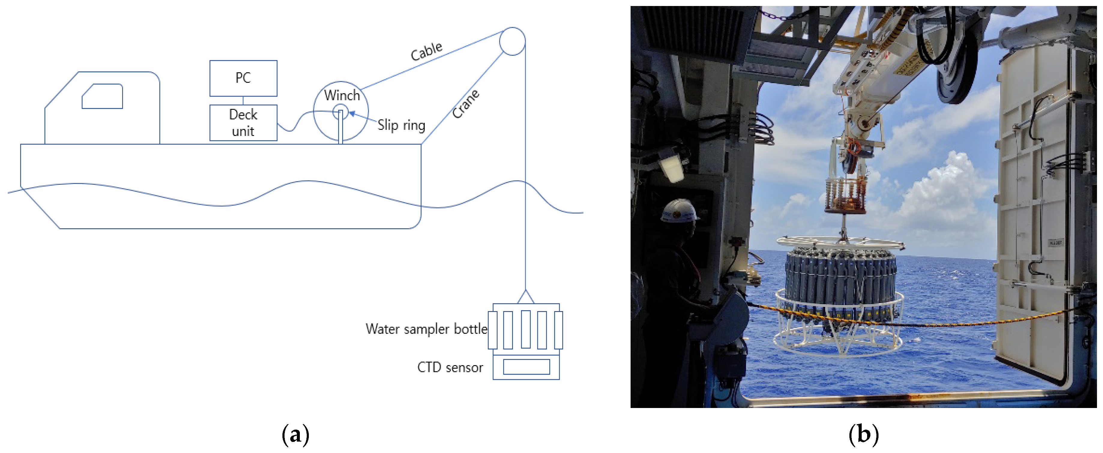
Figure 1. Overview of CTD system on the research vessel Isabu. (a) CTD system diagram; (b) an observation using a CTD system on the Isabu.
Jmse 12 00807 g001
Figure 2. The observation locations by using the CTD system on the research vessel Isabu. The sea area from which the CTD data were obtained is indicated by a blue circle.
Jmse 12 00807 g002
Figure 3. Acquired dataset ratio; (a) the number of data by sampling locations; (b) the number of data by normal/abnormal.
Jmse 12 00807 g003
Figure 4. Types of CTD anomaly patterns in seawater temperature data. (a) The spike in the red box shows missing values. For visualization with missing values, it was shown as zero values. Missing values appear over the entire measurable range. (b) It is an anomaly pattern that exceeds the effective temperature range. The observed seawater temperature in the sea area cannot be below 0 degrees. It mainly appears when an electrical fault occurs in the system. (c) It is an anomaly pattern that exceeds the measured effective measurement range of the temperature sensor. The seawater temperature value that the temperature sensor can measure is up to 35 degrees. It appears mainly in the sea surface section. (d) A pattern of point anomalies in the observed temperature profile; it mainly appears when an electrical fault occurs in the system. (e) It is a collective anomaly pattern of the observed temperature profile. It mainly appears in the mixed layer.
Jmse 12 00807 g004
Figure 5. A profile of CTD data; acquiring date: 22 December 2019; location: N 17.17, E 141.11.
Jmse 12 00807 g005
Figure 6. Comparison graph of performance for anomaly detection experiments in the seawater temperature profiles; (a) The graph shows the F-1 score result of the proposed top 7 experimental cases with the baseline IQR model; our proposed machine learning experimental cases show better F1 score performance than the IQR model. (b) This graph shows the results of the comparison between the seven models with the highest performance F1 score among our proposed models.
Jmse 12 00807 g006
Table 1. Confusion matrix.
Predictive Values
Positive (1)Negative (0)
Actual valuesPositive (1)TP
(True positive)
FN
(False negative)
Negative (0)FP
(False positive)
TN
(True negative)
Table 2. Performance evaluation index values of baseline IQR models and F1 score top 7 proposed experimental cases; in the dataset column, scale represents the normalization of the dataset (range of 0–1). The scale and oversampling columns indicate whether the technique is applied, “x” means that the technique is not applied, and “o” means that the technique is applied. The oversampling column describes the name of the technique applied to the dataset and the ratio of the minority dataset to the majority dataset.
Classification ModelDatasetScore
Model TypeModel NameScale (0–1)Oversampling
(Augmentation)
Sensitivity
(Recall)
PrecisionF1 Score (Std.)AUROC (Std.)
Traditional method
(baseline)
IQRxx0.1530.1880.1680.523
(Hidden layer sizes)
MLP-1: (10)
MLP-2: (10,15,10)
MLP-3: (500,100,10)
MLP-2-S-30xSMOTE 30%0.8320.9370.882 (0.013)0.912 (0.013)
MLP-2-A-50xAE 50%0.8410.9140.875 (0.020)0.914 (0.009)
MLP-1xx0.8120.9360.869 (0.021)0.901 (0.015)
MLP-2xx0.8050.940.867 (0.019)0.899 (0.017)
MLP-2-S-50xSMOTE 50%0.8460.890.866 (0.011)0.914 (0.015)
MLP-2-A-75xAE 75%0.8140.9250.863 (0.019)0.901 (0.023)
MLP-3-A-75xAE 75%0.8210.9080.861 (0.018)0.903 (0.016)
Table 3. Comparison of generalization performance; # is the row number of the table. OCSVM-ND is a model trained using a normal class. OCSVM-ND is a model trained using an abnormal class. “Average” represents the average of all experimental cases. “All cases” means the entire combination of all oversampling technique datasets used in this study.
Classification ModelDatasetScore
#ModelScale (0–1)Oversampling
(Augmentation)
Sensitivity
(Recall)
PrecisionF1 Score (Std.)AUROC (Std.)
1IQRxx0.1530.1880.1680.523
2OCSVM-ND
(normal data)
xx0.4750.1390.2150.501
3OCSVM-AD
(abnormal data)
xx0.5080.1280.2050.476
4MLP-1xx0.8120.9360.869 (0.021)0.901 (0.015)
5MLP-1-Sox0.6470.8440.729 (0.029)0.813 (0.025)
6MLP-2xx0.8050.940.867 (0.019)0.899 (0.017)
7MLP-2-Sox0.6760.8060.728 (0.02)0.823 (0.02)
8MLP-3xx0.8090.9150.856 (0.017)0.898 (0.018)
9MLP-3-Sox0.6360.7990.7 (0.047)0.803 (0.031)
10OCSVM-AveragexAll cases0.5030.1320.209 (0.007)0.484 (0.014)
11MLP-1-Averagex & oAll cases0.7570.760.735 (0.106)0.844 (0.055)
12MLP-2-Averagex & oAll cases0.7550.7740.751 (0.104)0.853 (0.051)
13MLP-3-Averagex & oAll cases0.7380.7530.719 (0.099)0.836 (0.051)
14MLP-ALL-AveragexAll cases0.8050.7890.77 (0.127)0.867 (0.062)
15MLP-ALL-AverageoAll cases0.6950.7350.701 (0.053)0.822 (0.025)
16ALL-D-Averagex & oAll cases of
duplication
0.7330.6980.694 (0.248)0.812 (0.164)
17ALL-R-Averagex & oAll cases of
uniform random
0.7130.5350.562 (0.183)0.756 (0.118)
18ALL-S-Averagex & oAll cases of
SMOTE
0.723 0.698 0.687 (0.203)0.807 (0.135)
19ALL-A-Averagex & oAll cases of
AE
0.694 0.734 0.685 (0.209)0.795 (0.139)
Disclaimer/Publisher’s Note: The statements, opinions and data contained in all publications are solely those of the individual author(s) and contributor(s) and not of MDPI and/or the editor(s). MDPI and/or the editor(s) disclaim responsibility for any injury to people or property resulting from any ideas, methods, instructions or products referred to in the content.