The Role of Different Total Water Level Definitions in Coastal Flood Modelling on a Low-Elevation Dune System

Abstract

The present study investigates different combinations and methods for estimating the extreme Total Water Level (TWL) and its implications for predicting flood extension caused by coastal storms. This study analyses various TWL components and approaches and assesses how different methodologies alter flood predictions, with implications for warning systems and emergency responses. Using different combinations of individual TWL components, flood extension simulations were conducted using a hydrodynamic model in the Volano Beach area (Emilia-Romagna, Italy). A real coastal storm event was used as a reference for comparison. The findings indicate that the selection of individual TWL components and calculation methods significantly impacts flood extension predictions. The approaches, which involve calculating extreme values from a combined time series or the water level time series plus the extreme value of wave setup, yield the most realistic results, excluding the runup component. In comparison, the other combinations overestimate the flood. Incorporating hydromorphological models like XBeach could enhance the accuracy of runup estimations and improve the overall method reliability. Despite limitations such as runup estimation and the use of generic regional parameters, this study underscores the importance of the TWL combination selection in accurately predicting flood extents, emphasising the need for context-specific adaptations in environmental contexts.

1. Introduction

Coastal storms can significantly impact coastal areas, causing shoreline erosion and flooding, damaging infrastructures, and, at worst, even causing human injuries, including death. Coastal hazards generated USD 364 billion in losses in the USA from 1960 to 2014 [1]. With the predictions of the world’s population increase in coastal areas [2], the risk associated with these events also increases, leading to the need to predict and understand the processes that can contribute to coastal flooding. Numerical models can be used to provide crucial information to understand, predict, and, therefore, mitigate the impacts of coastal storms. Their development and availability have increased over the last decades, covering different areas: XBeach [3] and D-Morphology [4] for the analysis of morphodynamic changes, SWAN [5], WWIII [6], and FUNWAVE [7,8,9,10] for wave dynamics, Lisflood-FP [11,12,13], ROMS [14], SCHISM [15], TELEMAC [16], MIKE 21/3 [17], and D-Flow FM [4] for flood propagation. These numerical models can also be valuable tools if used in operational mode in support of early warning systems, providing relevant information for local authorities, such as flood extension or morphological impact, prior to the event. Among them, Lisflood-FP has been widely applied in studies of coastal flood propagation [12,18,19,20,21,22,23,24], as it uses simple shallow water equations to represent the dynamics of the flood event. An example of the usage of this model to simulate possible extreme scenarios was presented by Vousdoukas et al. [19], who simulated the propagation of floods related to low-frequency (100-year return period) events in Europe, showing good accuracy compared to satellite imagery. Similarly, in the EU H2020 ECFAS project (www.ecfas.eu, accessed on 13 June 2024), a flood catalogue for European coastlines was created using Lisflood-FP, which predicted the propagation of coastal floods during extreme events of low and medium frequency, once again showing reliable results when compared with satellite imagery and local flood markers [18]. However, Paprotny et al. [25] show that although pan-European models simulate with adequate accuracy certain parameters, such as storm surge heights, large-scale flood maps have large disparities when compared to local scale maps.

Although numerical modelling provides useful information when using the forecasted conditions as input, they may entail an extended computational time and require an interpretation of the results, which can take a long time and could be crucial in delaying the responders’ decision while the event is taking place. Therefore, the creation of event maps using the same numerical models but covering a wide range of boundary conditions of possible events as input is a solution that is often used [18,26,27]. The generation of a catalogue covering possible events in an area can be used to provide a warning level for a specific event simply by selecting a flood model map from the catalogue. Through pre-established warning levels, the authorities’ response time could be faster since there is no need to wait for numerical model outputs and interpretation.

In order to trigger the different warning levels, thresholds need to be defined according to the predicted intensity of the event. The establishment of thresholds and identification of extreme levels, which can be carried out by employing the Total Water Level (TWL), has been done through different studies with varying objectives. The TWL at the coastal boundary is one of the most important factors that needs to be considered when studying and predicting the flooding of coastal areas. According to the equation developed by Pugh [28] TWL can be defined as follows:

TWL(t) = Z0(t) + T(t) + R(t)

(1)

The TWL is defined by three components: the mean sea level (Z0(t)), the tidal component (T(t)), and the non-tidal residuals (R(t)), which includes wave setup and storm surge, among other phenomena [1]. The inclusion or representation of different components of the non-tidal residual (R) opens the door to multiple combinations using different variables, resulting in varying values of TWL. This variability in the choice of the inputs has been demonstrated in many studies: Vousdoukas et al. [19,29] and Le Gal et al. [18] use the mean sea level, the tide, and the wave setup to establish the TWL for flood extension prediction; Jiménez et al. [30] use wave information for the inundation vulnerability of the Emilia-Romagna region; Del Río et al. [31] used an approach, which, even if it was not focused on coastal flooding, calculated the TWL, including the tide level, wind-induced setup, barometric setup, and wave-associated sea level variation; Rulent et al. [32], Croteau et al. [33], and Caruso and Marani [34] considered the TWL to be the mean sea level, tides, and storm surges, excluding the wave parameters. On several occasions, the wave and atmospheric contribution are not jointly taken into account, not even at a probabilistic level. In recent years, the copula theory has become the standard for joint probability estimations for flooding, with a local application even for the regional area where this study is located [35]. However, one of the limitations of such advanced statistical methods is the availability of simultaneous and long-time series of waves and water levels.

The components used to define the TWL are critical aspects that can significantly change the TWL values. The variations in the TWL due to the components are strongly related to the geographical region and vary according to the oceanographic and meteorological setting (e.g., wave climate, tidal range, and exposure to low-pressure weather systems). Furthermore, the method used to define an Extreme Value (EV) can influence the TWL extreme values and, therefore, the definition of thresholds, which also depends on the frequency of occurrence of the extreme event (return period). When applied to flood modelling, the different approaches used to calculate the TWL and the associated extreme values can have implications that need to be understood. This study analyses the effects of the inclusion of different components to calculate TWLs, the use of different methods to obtain TWL extreme values, and the resulting implications for numerical flood modelling. Based on the extracted extreme values, simulations of flood extension were applied, using Lisflood-FP, to understand how the different TWLs influence the results. The different TWL combinations and methods were tested on an urban coastal area of the Emilia-Romagna coast (Italy) on the Adriatic Sea. The coast of this Italian region has been highly affected by coastal storms [36,37,38,39], and their consequences are particularly significant due to the dense urbanisation, especially in cases where infrastructures are built on top of/or behind low-lying dunes [40].

2. Study Area

This research was conducted at Lido di Volano, situated in the Emilia-Romagna region (Figure 1). The region’s coastline is characterised by dissipative beaches, with slope values around 0.03 [40]. On average, the maximum elevation of the back-shore is 1.45 m above mean sea level (MSL) [40]. The anthropic pressure in the Emilia-Romagna region is high; urbanisation covers 71% of the 130 km of coastline [40], and 43.86% of the coast has dune systems [41]. During modal wave conditions, the region is characterised by waves from the east, but during high-energy events, waves have an ENE direction. Generally, wave heights are below 1.25 m, while significant wave heights can reach 2.5 m during storms, with an event duration usually lower than 24 h [40]. Although strong winds that affect the region are from ENE, the winds that cause the highest surge events are the SE winds (Scirocco), which are usually weaker [38]. The increase in storm surge with these winds is associated with the orientation of the coast and can reach 0.6 m for storms with return periods from 1 to 2 years [42]. The area is characterised by microtidal semidiurnal conditions, with the tidal range reaching 30–40 cm during neap tide and 80–90 cm during mean spring tide [40].

The strong human influence and the low-lying dune systems favour the area being exposed to floods and damages by coastal storms, whose impact is well-known [36,37,38,39]. The stakeholders carry out specific actions to protect the coast from high-energy events in the area, such as creating artificial dunes to protect private properties [40].

Volano village (Figure 2A), which represents the typical coastal beach resort of the Emilia-Romagna region, is characterised by low-lying dunes and high anthropic pressures on the beach area through the construction of permanent installations like beach huts, bars, etc. Also, the beach profile is constantly altered during the summer season when users flatten the beach to arrange as many beach umbrellas as well as deck chairs. Due to the dune characteristics, there is almost no front line of natural protection, leading to a frequent impact on the buildings due to extreme coastal events, including restaurants at the beach and on the backshore. According to historical records, it has been one of the areas of the region most affected by storms in the last 50 years [43].

The extreme event chosen for this study occurred on the 22nd of November 2022 [44] and impacted the Emilia-Romagna region’s natural and urban areas in the northern part of the coast, where the study area is located. The TWL registered by the tide gauge of Porto Garibaldi (Agenzia Prevenzione Ambiente Energia—ARPAE) reached values of 1.48 m above the MSL (Figure 3), the highest recorded values since it was installed in 2009, where 1 m was due to the storm surge [44]. The most important previous event, the Saint Agatha storm (2015), characterised by a TWL of 1.21 m at the same tide gauge, was considered by Perini et al. [37] an event with a return period of 100 years. The event of November 2022 was mainly driven by atmospheric factors combined with spring high tide. Although wave height reached 3 m in front of Volano, higher than the value established by Armaroli et al. [40] for causing inundation and damage to anthropogenic areas (above 2 m), it was smaller compared to the previous Saint Agatha Storm, which led to extensive damage to the region and had a wave height of 4.66 m [36,37].

Furthermore, although the TWL value was significant, the event’s effect in Volano was even greater due to the breach of a dike NE of the city. The flooding of the urban area was not the focus of this study, but this event was selected as a reference event because it had a peak water level higher than the established return period of 100 years. It was used in comparison with synthetic storms, using different possible extreme total water levels.

3. Datasets

3.1. Definition of the Total Water Levels

Different sources were used to collect the data to calculate the TWLs. Water level and wave data were retrieved from a dataset containing a 27-year hourly sea level and wave hindcast (1994–2020) over the Northern Adriatic Sea [45] with a resolution of 0.025° and a RMSE between 7.9 to 15 cm for the water level and 18 to 34 cm for the waves, which was produced using the SHYFEM [46] and WAVEWATCH III [6] models forced with the wind data from the European Centre for Medium-Range Weather Forecasts (EWCMWF) reanalysis version 5 as input. The tide information was obtained from the pyTides2 Python library (https://pypi.org/project/pytides2/, accessed on 13 June 2024). The MSL was referred to the Italian national datum of Genova 1942. The residual was calculated by subtracting the predicted tidal elevation from the offshore water level time series, and the nearshore components were computed using the Stockdon et al. [47] equation using the wave time series. The dynamic runup component was calculated by subtracting the wave setup value from the wave runup value obtained by the Stockdon et al. equation [47].

3.2. Inundation Modelling

Three main inputs that were used in the setting up of the flood model to estimate the flood extension were topographic data, Land Cover/Land Use (LC/LU) and water level information. The topographic data used was a 5 m resolution Digital Terrain Model (DTM) from 2018, available from the GeoPortale of the Emilia-Romagna Region (Figure 2B). The Land Use/Land Cover of the coastal zone (2018 version) was provided by the European Environment Agency [48,49] as a part of the Copernicus Land Monitoring Service. It classifies the different land areas according to their characteristics, attributing one of seventy-one available classes. The land-use classes can be converted into bed friction classes by applying Chow [50] and Papaioannou et al.’s. [51] work, where the area’s land cover classes were associated with a specific Manning coefficient (0.013 s m^−1/3 for urban and transport infrastructures areas; 0.1 s m^−1/3 for Coniferous and Broadleaved forest; 0.04 s m^−1/3 for grassland; 0.03 s m^−1/3 for permanent crops). There were two main inputs for the water level information: the TWL obtained by the analysis of extreme values or the TWL from the November 2022 Volano event. The November 2022 event data was obtained from the Porto Garibaldi tide gauge located on the coastline of the Ferrara province (Figure 1). The wave information data of this event was retrieved from the offshore position 44.669° N 12.470° E using the Copernicus Marine Environment Monitoring Services (CMEMS) regional wave forecast [52] (the hindcast data was not available at the time when the work was performed).

4. Methodology

The following sections present the different terminology used in this study, the selected components for the determination of the TWL, the methods used for the determination of the extreme values of each component or time series, the possible combinations using the different components’ extreme values, and an explanation of the process used for the determination of representative values for each possible combination. Furthermore, the application of the numerical model to simulate extreme events, both realistic and synthetic, is described.

4.1. Definitions

For a better understanding and clarity of the current study, some term definitions are necessary.

• Component: the representative value of one or more components of the total water level. The components can be either static or dynamic according to their nature. They can also be divided into three categories according to the method used to calculate the extreme value;
• Static Component: a component whose variability in time is limited and whose physical behaviour can be represented by a static (fixed) value;
• Dynamic Component: a component whose value cannot be represented correctly by attributing a fixed value. The only component in this category is the dynamic runup.

An extreme value can be obtained directly from an analysis of the time series (see Section 4.2.1) or calculated indirectly by applying the extreme values referent to other variables of an equation. Hence, it was necessary to distinguish the methods used to obtain the extreme value. Three categories were defined according to the method used to obtain the extreme value of the component: (i) Base, (ii) Univariate, and (iii) Estimated (

Table 1. Type and description of the components used to calculate the extreme values of total water level.

Component	Base	Univariate	Estimated
MSL	Local (0 m)	-	-
Tide	MHW: Mean High Water
	MHWS: Mean High Water Springs	-	-
	HAT: Maximum Astronomical Tide
Residual	-	Time series (water level—tide time series)	-
Setup	-	Stockdon et al. [47] time series	Stockdon et al. [47] Single value
Dynamic Runup	-	Stockdon et al. [47] Runup-Setup, time series	Stockdon et al. [47] Runup-Setup, Single value
Water level	-	Time series (Residual + Tide)	-
TWL static	-	Time series (water level + setup)	-
TWL dynamic	-	Time series (water level + setup + dynamic Runup)	-

). The Base category contains the components considered immutable in the case of an extreme event and, therefore, are fixed (i.e., the MSL and tidal components). The Univariate category refers to the values directly obtained by applying the extreme analysis of a specific component to the time series. This category can be applied to all the components besides the base type components (MSL and Tide). The Estimated variable refers to the indirect method used to calculate the extreme value, which means using the extreme value from a dataset (e.g., wave time series) to calculate the extreme value of a component (e.g., setup or dynamic runup). This can only be applied to the nearshore components, the only components for which the extreme values can be obtained by using the extreme wave height values on the Stockdon et al. [47] equation, which requires two extra variables: the peak wave period and the beach slope. The offshore peak period (Tp) was calculated using an empirical solution developed by Duo et al. [53] for the Emilia-Romagna coastline during extreme events employing the offshore significant wave height (Hs) obtained by long-term measurements at the Cesenatico buoy:

Tp(s) = 1.32 × Hs(m) + 3.86

(2)

The applied beach slope was 0.03, which Armaroli et al. [40] defined as the mean value for the Emilia-Romagna region.

4.2. Extreme Event Analysis

4.2.1. Extreme Value Analysis

Extreme event regularity can define an extreme event [54], meaning that if an event has a certain extreme value, it will correspond to a certain return period. A wide range of return periods were selected to identify the TWL values of extreme events corresponding to different frequencies: 1, 2, 5, 10, 20, 30, 50, 100, 300, and 500 years.

The extreme values for the selected return periods were calculated using the Python library pyextremes (https://georgebv.github.io/pyextremes/quickstart/, accessed on 13 June 2024). A Peak-over-Threshold (POT) analysis was used to discriminate between extreme events. This method uses two variables that need to be defined: threshold and independence criteria (i.e., the period that separates two different storms). A range of values was selected for these two variables: the percentiles 0.97, 0.98, 0.99, 0.995, and 0.99 for the threshold and 12, 24, 48, and 72 h for the independence criteria. The different range of values was applied to assemble all the general possible configurations in order to identify extreme events. Afterwards, they were filtered according to certain characteristics with the aim of obtaining only one configuration. The filtering process was divided into two phases:

• Number of extreme events per year. Based on the literature and local studies, the area of Emilia-Romagna is affected by 2 to 6 storms per year. If the results of the combinations of variables for the EVA did not fit this range, it was not considered for the final analysis;
• Statistical values of Pearson r PP and QQ. The pyextremes package provided statistical values of extreme events analyses, in which Pearson r PP and QQ are included. If the statistics’ values were considered statistically representative (>0.97), the extreme value was included in the analysis of TWL.

4.2.2. Total Water Level Combinations

The extreme values obtained from the EVA were used in three ways to obtain the TWL extreme value: (i) aggregation of each individual extreme value of the component; (ii) direct use of the extreme value obtained by the EVA of a combined time series (which aggregates all the components time series), via the method based on Sanuy et al. [55]; (iii) aggregation of the extreme value of individual components and an extreme value of a combined time series (water level).

The four variables included in all the TWL-tested combinations were the MSL, tide levels, residual and wave setup. The value attributed to the MSL is 0, and the tide varies between the Mean High Water (MHW), High Mean Water Springs (MHWS), and the Highest Astronomical Tide (HAT) or the usage of the complete tidal time series. The residual and the wave setup are included as extreme values or a part of the combined time series (i.e., total water level time series).

All the combinations have two versions, with (dynamic combination) and without (static combination) the dynamic runup. The dynamic runup is either calculated separately and added to the final values or is part of a combined total water level time series. Depending on the variables included in the TWL calculation and the final extreme values method, an acronym is attributed to the combination. The resulting eight combinations and the acronyms used for each one are specified in

Table 2. Definition of the different TWL combinations. The straight brackets represent the extreme values from a combined time series. If not in the brackets, the extreme value is from the component’s time series.

TWL Acronyms	Used Component
dCUE	MSL (base) + Tide (Highs) + Residual + Estimated nearshore components (setup and dynamic runup)
dCUU	MSL (base) + Tide (Highs) + Residual + Univariated nearshore components (setup and dynamic runup)
dTU	TWL dynamic [MSL (base) + Tide (Highs) + Residual + Univariated nearshore components (setup and dynamic runup)] Based on Sanuy et al. [55]
dWUU	Water Level [MSL (base) + Tide (Highs) + Residual] + Univariated nearshore components (setup and dynamic runup)
sCUE	MSL (base) + Tide (Highs) + Residual + Estimated Setup
sCUU	MSL (base) + Tide (Highs) + Residual + Univariated Setup
sTU	TWL static[ MSL (base) + Tide (Highs) + Residual + Univariated setup] Based on Sanuy et al. [55]
sWUU	Water Level [ MSL (base) + Tide (Highs) + Residual] + Univariated Setup

.

4.2.3. Selection of Representative Values

To represent the different intensities of the events, the return periods were divided into three distinct categories of frequency: (i) high [return period: 1–20 yrs], (ii) medium [30–50 yrs], (iii) and low-frequency scenarios [100–500 yrs]. This means that the high-frequency events correspond to the most common ones, while the low-frequency events correspond to the most intense and unusual events. Since a high amount of return periods are available, selecting a single value can increase the uncertainty of the method. Hence, the Monte Carlo approach was applied, choosing three values for each variable related to the respective frequency (nine in total) while considering the predefined MSL and tidal levels. Afterwards, those values were combined in all possible ways. The Monte Carlo simulation was used to select the final extreme values of the TWL, which wound up corresponding to a low, medium, and high value for each frequency. Note that the combined TWL time series process (TU) will only be feasible one time via the Monte Carlo method after the final extreme values of the combination thus far have been calculated.

4.3. Flood Model Configuration

Lisflood-FP [11] is a hydrodynamic model dedicated to simulating the propagation of a flood using a variety of numerical schemes to solve 2D shallow water equations. The model uses high-resolution raster Digital Elevation Models, and it has been used in different fields of hydraulic modelling [13]. As input data, the Lisflood-FP model needs a 2D grid with the topographic information, the values of friction and infiltration, and the boundary points with the water level information. The area represented in red in Figure 2A defines the numerical domain, and the data retrieved from the Emilia-Romagna Region DTM (Figure 2B) was used (See Section 3.2). In the case of terrain friction, a grid with the same dimension as the DTM was created, incorporating friction values for each cell. The boundary points where the water level time series was implemented were located at a height of 0.25 m with a spacing of 1 m. For infiltration, the value for low-density residential areas (6.44 × 10⁻⁶ m/s) was used [56]. The numerical floodplain solver applied was the “acceleration” one, considering previous good performances in coastal areas and its computational efficiency, as proved in previous works [12,18,57,58,59,60]. The increase in the computational efficiency of the floodplain solver acceleration solution is obtained through a simplification of the shallow-water equations by disregarding the convective acceleration terms.

Two different types of events were simulated: synthetic events considering several TWL component combinations and using the real event of November 2022 (Figure 3), using the TWL extracted from Porto Garibaldi’s tide gauge (Figure 1). The real event was also simulated considering the runup effect using wave time series from CMEMS, Stockdon et al. [47], peak period [53] equations, and the representative beach slope for Emilia-Romagna beaches.

Synthetic storms (Figure 4) were modelled using a triangular time series. The triangular-shaped time series method has been used in previous works [18,61] despite the limitations noticed by Duo et al. [53] regarding the accuracy of the representation when compared to realistic cases. The initial (0 h) and the end (6 h) values of the TWL time series used corresponded to the value of the mean tide (0.31 m), calculated from the tide time series from the pyTides2 python library (Section 3.1). The peak, in the middle of the event following a symmetric triangle (3 h), corresponds to the TWL value extracted from the extreme value analysis (Figure 4). The time step for the TWL data used as an input for Lisflood-FP was 30 min.

The simulations applied in this work used as boundary conditions were (i) the two TWL time series of the real storm (one including the runup and the other excluding it), and (ii) the 24 synthetic storm scenarios (eight for each frequency scenario). This analysis compared the flood extension between synthetic and real event scenarios. The last ones were used as a reference to see which TWL combination was preferable when predicting a storm with a high impact on the coast.

5. Results

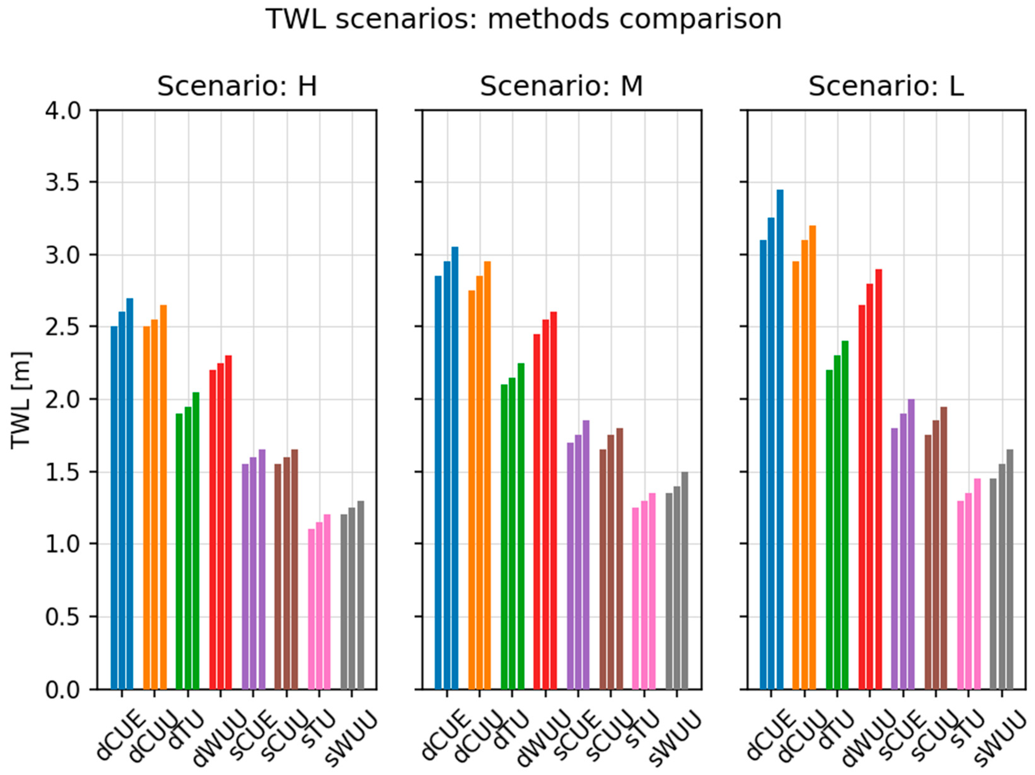
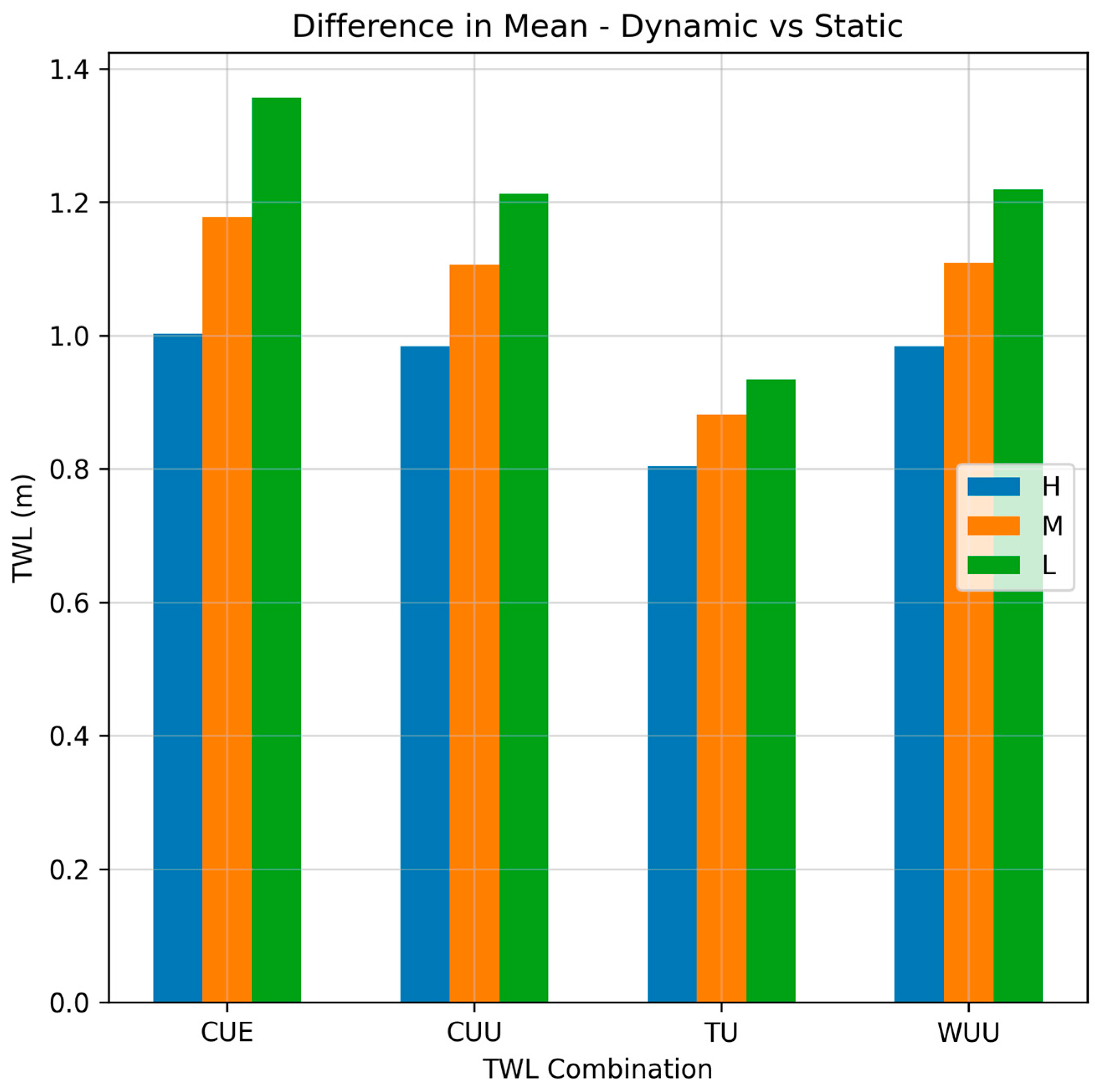
5.1. Nearshore Total Water Levels

Seventy-two representative TWL extreme values were extracted from the extreme value analysis of the TWL combinations (See Section 4.2) (Figure 5) and divided into three different categories (24 each) based on the frequency scenarios (High, Medium, and Low) and then three representative values of each combination. The direct comparison between scenarios demonstrates that the magnitude pattern for each combination is similar, but the dimensions vary: the lowest to highest results remain the same between the three scenarios. The combinations that show the highest and lowest values of the TWL in every scenario were the dCUE and sTU (Figure 5), which consider the MSL, the tide, the residual, and the estimated nearshore components extreme values separately, and the extreme value of a time series that combines the MSL, the tide, the residual and the univariate setup, respectively (Table 2). The highest representative values of the dCUE and sTU (which correspond to a low-frequency event) were 3.55 m and 1.45 m, respectively, which corresponded to a difference of more than 2 m of the TWL. On the other hand, the lowest values (high-frequency event) were 2.5 m for the dCUE and 1.1 m for the sTU.

In each scenario, the contrast between the static and dynamic versions of the combinations was noticeable (Figure 6). The highest difference between the versions (dynamic and static) corresponded to the CUE combinations, with a 1.36 m difference in the low-frequency scenario, while the lowest corresponds to the TU in the high-frequency scenario, where the difference was 0.8 m. Also noticeable was the increase in the difference with the decrease in the frequency of events; the high-frequency events showed the lowest difference between static and dynamic, and the low-frequency events showed the highest difference for each combination.

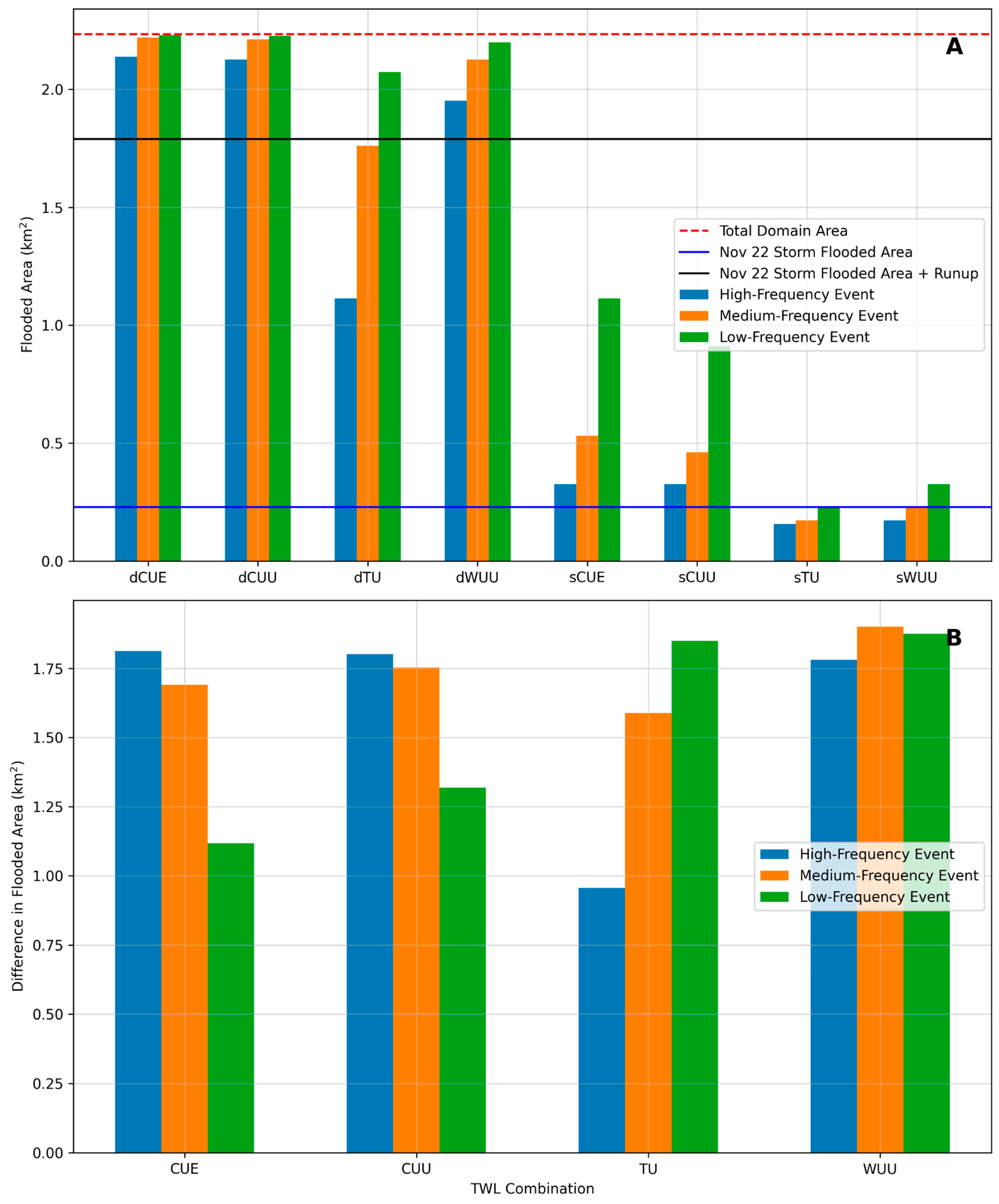
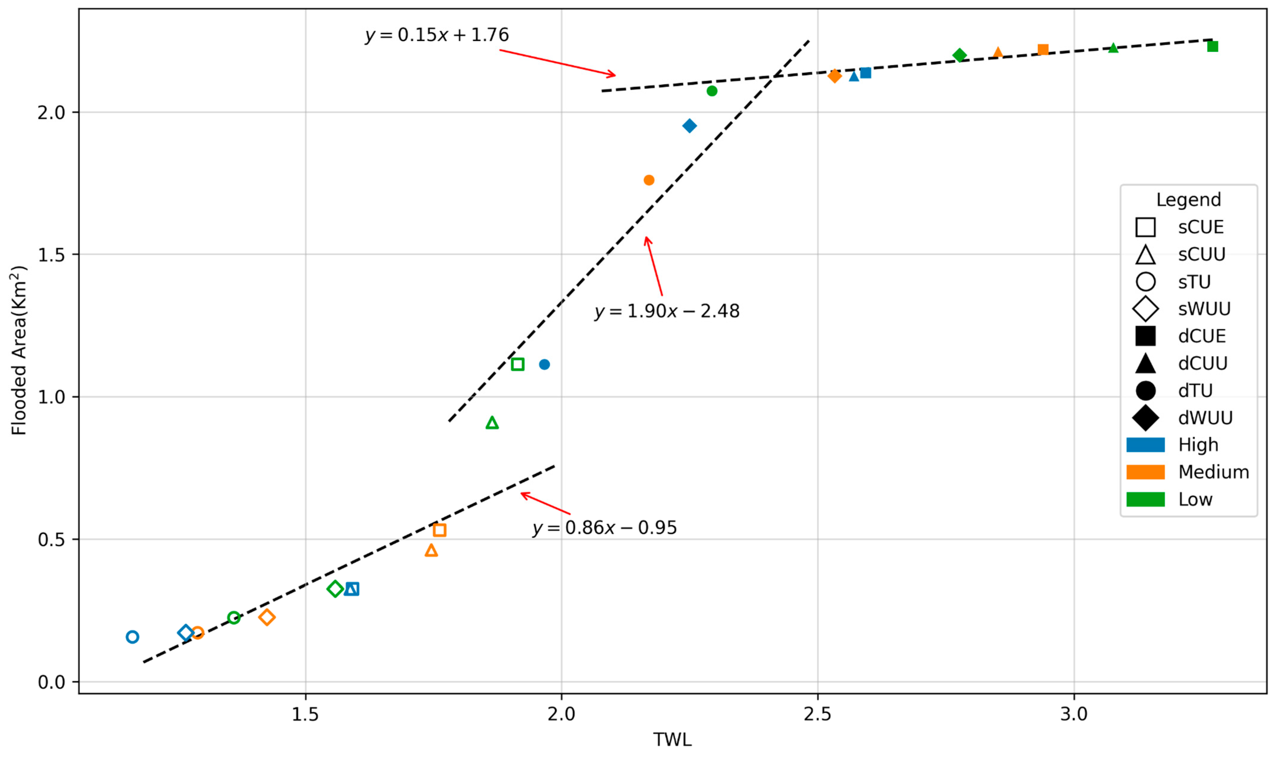
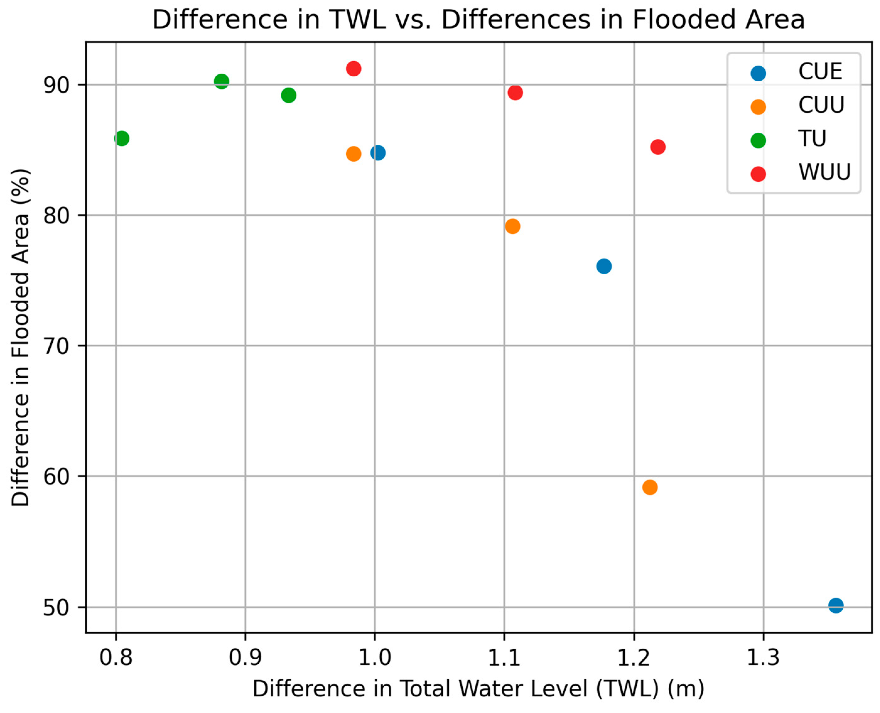
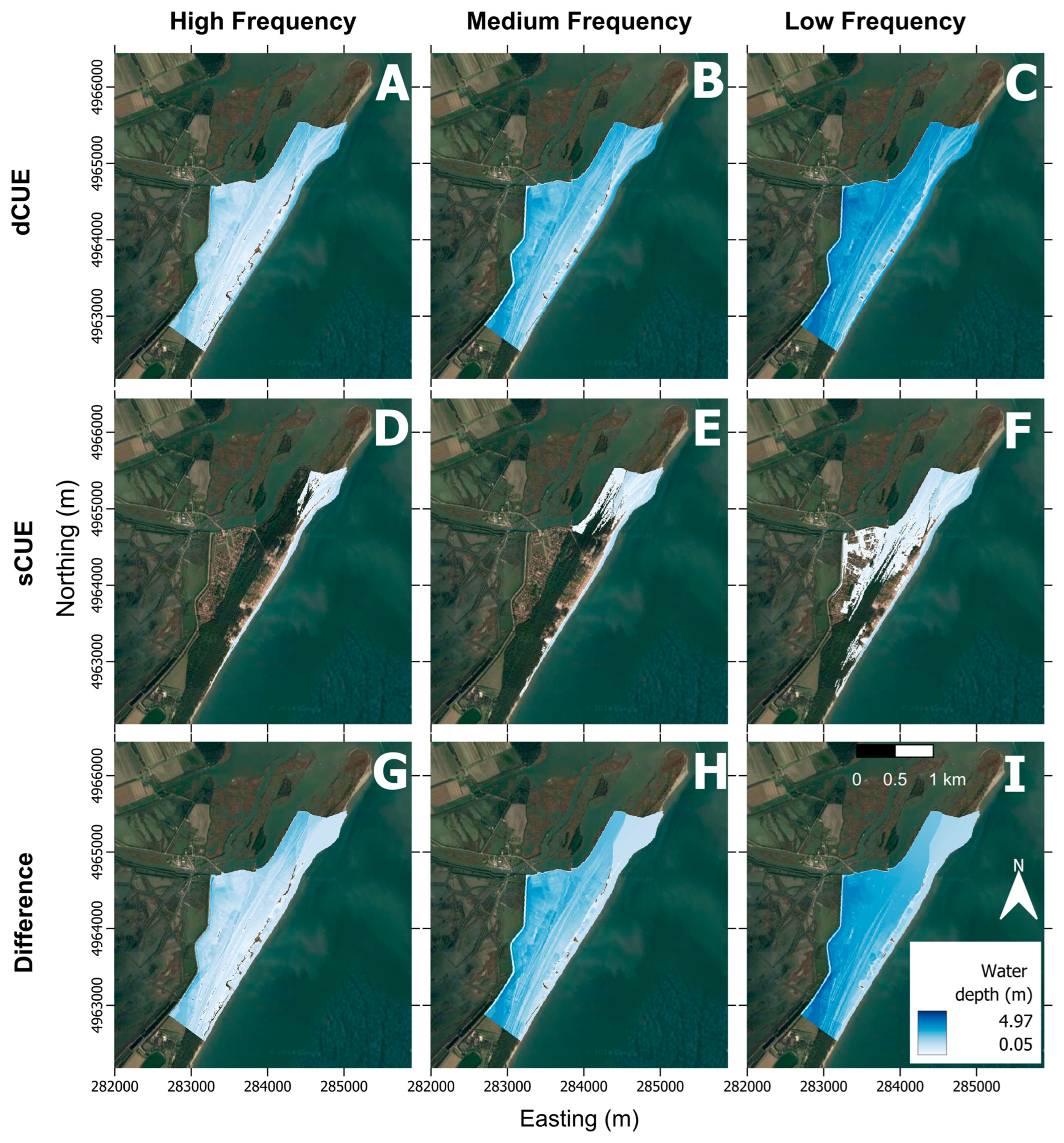
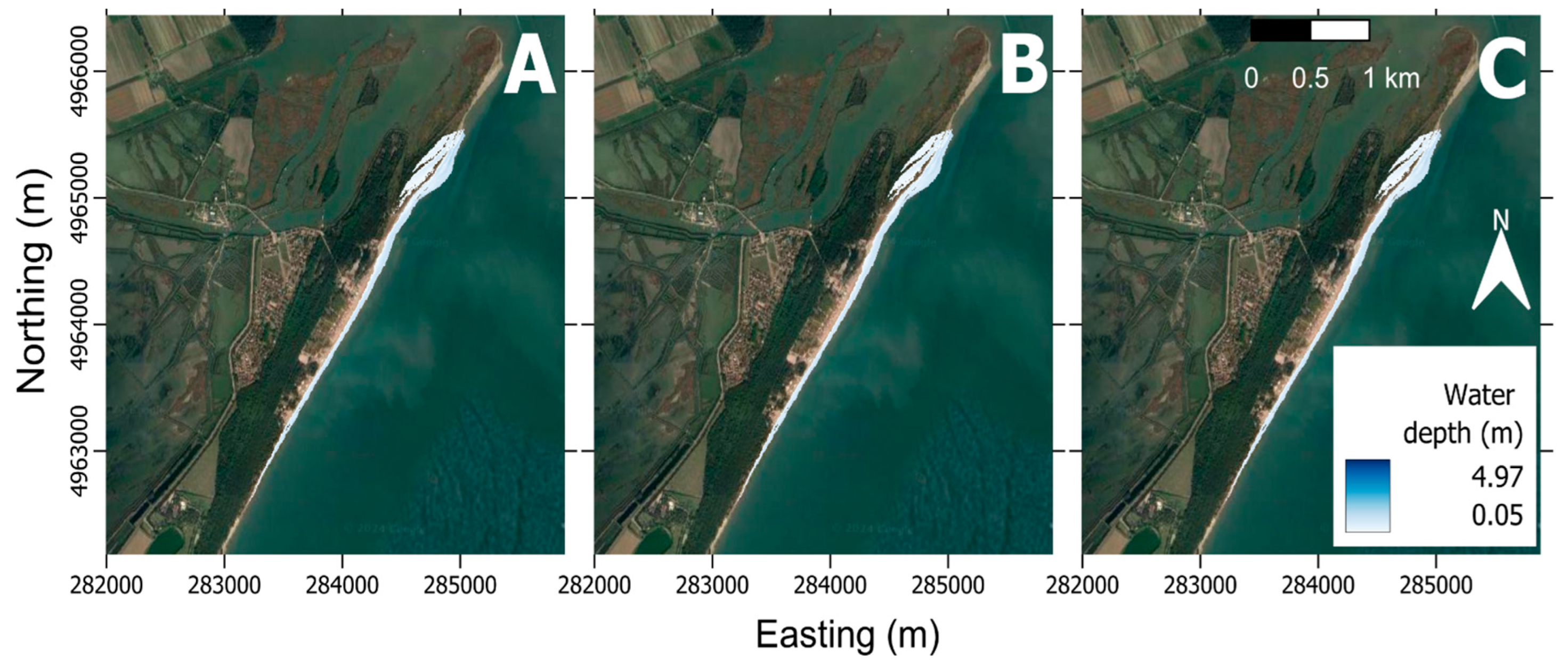
5.2. Flood Extension Analysis

In taking into account the synthetic storms calculated with different combinations of TWL components and the real event, flooded areas were generated using the Lisflood-FP model (26 in total). Figure 7A demonstrates that various TWL combinations in different intensity events either reach or are close to reaching the maximum area of the numerical domain. In fact, that condition was achieved only in the dynamic versions of the combination, and it was achieved independently from the intensity of the event for the dCUE combination. While the static versions of the combinations reached a much lower flooded area, the highest flooded area of the static combinations (low-frequency sCUE) reached the lowest values of the flooded area (high-frequency dTU). The difference between dynamic and static versions of the combinations is better demonstrated in Figure 7B, which illustrates the direct comparison between the versions and their respective frequencies, with the lowest difference of flooded area corresponding to the high-frequency TU combination (0.96 km²) and the highest to the medium-frequency WUU (1.90 km²).

In Figure 8, the relation between the TWL and the flooded area is represented and three different stages of the relation between the flooded area and the total water level can be observed. The first (using low TWL values, corresponding exclusively to the static combinations) showed a low impact on the flooded area. The second one, after a certain point, demonstrated the increase in velocity of the flooded area (a low increase in TWL has a greater impact than the first stage). The third and final stage of TWL–flood relation (represented only by the dynamic combinations) started out slower with the limitation of the total area of the numerical domain.

Figure 9 visualises the impact of the difference in the TWL between static and dynamic versions and the percentage difference in flooded areas for each method. The TU and WUU showed higher differences in flooded areas between the static and dynamic versions, constantly increasing from 80% to 90% of flooded areas when increasing with the TWL. However, the CUE and CUU combinations showed a reduction in the impact of a greater TWL. In fact, the highest value of difference in the TWL corresponded to the lowest percentage, reinforcing the limitation shown in Figure 8. Nevertheless, the difference in the flooded area impacted was at least 50% when comparing the static and dynamic versions.

As previously mentioned, the TWL combination that resulted in the highest TWL values was the dCUE (Figure 7A), which considered the dynamic runup; the flood extension covered the entire village of Volano for all scenarios, as can be observed in Figure 10A–C, where the whole numerical domain was flooded. The flood extension was considerably reduced for the same TWL component combination (Figure 10D–F) when the dynamic runup was not considered (sCUE), although Volano was still highly impacted by the flood in the low-frequency event (Figure 10F). Figure 10G–I makes it possible to visualise that even in the cells that were flooded by both combinations, the static and dynamic CUE, have a big difference in water depth. This can also be due to the limitation of the numerical domain, which does not allow the exit of the accumulated water and, therefore, impacts the water depth of the cells.

As described in Section 2, the event of November 2022 was used as a reference to analyse which combination better represents the flooding process in the Emilia-Romagna area. When analysing this storm, taking the runup into account, the dynamic combination’s synthetic storms overestimated the flooded area apart from the high and medium-frequencies of the dTU method, the last one being the closest to the simulation of the event with dynamic runup (Figure 7A). However, a high correspondence was found between the flooded area of November 2022 without the runup, the sTU low-frequency, and the sWUU medium-frequency event. The same maximum flooded area, 0.23 km² for the three cases, was observed when simulating the real event and the two combinations mentioned (Figure 11).

6. Discussion

The results from the extreme value analysis showed that including the dynamic runup, in both univariate and estimated forms, significantly impacted the TWL of the extreme events, increasing, in some cases, the TWL by about 1.36 m when compared to the static version of the combination (Figure 5 and Figure 6). This difference also influenced the flood areas where the difference between the static and dynamic versions could reach 1.9 km² (Figure 7B), and range from not impacting the city area to flooding it completely. The relation between the TWL and the flooded area (Figure 8) behaved in three different ways, with a low influence of the TWL and flooded extension up to a certain level, but after a threshold, the small increase in the TWL affected greater impacts. This confirms the finding of Lyddon et al. [24], who, using Lisflood-FP, concluded that after a flooded threshold, differences of a few centimetres could cause an increase in the flooded area and, consequently, greater damage. The third stage of the TWL–flood relation developed more slowly because it was limited by the total area of the domain. This demonstrated a high degree of impact on the results, and we can see that the results of the dynamic models were limited by this domain area. The WUU method, independently of the frequency, showed an almost constant increase in the flood area from static to dynamic (see Figure 7B). This occurred because the inclusion of the extreme dynamic runup had an impact of >80% (Figure 9) on the TWL, transforming the flooding of the beach and forest area into a complete flood according to the numerical domain in the case of the WUU. In a separate case, the TU showed different increases in the different flooded areas between versions during the increased intensity of the event (Figure 7B), with increases of >80% (Figure 9), similar to the WUU; however, it impacted almost the total numerical domain during only the most intense event. The CUE and CUU presented a linear decrease between events due to the fact that the static versions of medium and low-frequency events were already impacting a high amount of area of the numerical domain. Therefore, when including the dynamic runup, the flood extended to the total numerical area, flooding every grid cell. In contrast, the increase in the TWL did not translate into an increase in the extension of the flooded area due to the numerical area limitation. Figure 9 demonstrates this decreasing percentage of flooded areas with the increase in the TWL. Nevertheless, the impact of the dynamic runup was visible when comparing the static and dynamic versions (Figure 7A and Figure 8), allowing the storm to reach an inundation regime [62] in various frequencies and combinations. The impact of the dynamic runup and its importance are well known, and their exclusion can create an underestimation of hazard and occurrence [63]. In many cases, authors often avoid runup considerations [18,19,31,34,64], maybe due to the lack of data regarding the waves and nearshore area or to uncertainties in the results, as has been observed in this work in the modifications from the static to dynamic. In previous works, such as that by Le Gal et al. [18], where a flood catalogue was developed using extreme values of the TWL, or that by Voudouskas et al. [19], which simulated an extreme TWL for 100 yr return period scenarios; only wave setup was included among the nearshore values. Similarly, the current definition of the scenarios of nearshore TWLs adopted by the Emilia-Romagna Region for prevention and response management only includes the wave setup, thus excluding the dynamic runup (the dynamic component).

Not only are the differences between static and dynamic versions of the combinations relevant, but the difference between methods of calculating the TWL extreme values is also significant. Even if the dynamic runup is not included in the combinations of accumulating the different components (sCUE and sCUU), their extreme values create a flood that would impact the city of Volano for the lower-frequency occurrences (Figure 10). The analysis of the flood extension was made considering the storm of November 2022 as a reference for the simulation of a synthetic storm. As shown in Figure 7A and Figure 10, the dynamic combinations will create a value that would impact the whole area of Volano, even in high-frequency events. The only exception to this is the dTU combination. Serafin and Ruggiero [65] developed a model of simulation of the TWL that uses a similar combination to dTU, which demonstrated a higher value for the extreme event return periods in comparison with the observational data from the tide gauges, resulting in 5% more dunes to be overtopped during a 100-year event, this higher value may be due to a better temporal convergence of the model in comparison with the in situ methods. Including dynamic runup in the TWL as an individual value and not in a common time series creates an overestimation of the final extreme value of TWL and, consequently, an overestimation of the flooding area. In the case of the individual extreme value combinations (CUU and CUE), a low-frequency event would flood the city and partially impact the Lido di Volano, even without the dynamic runup component (Figure 10). According to the authorities of the Emilia-Romagna region, the values for high, medium, and low-frequency events are 1.5, 1.8, and 2.5 m, respectively. The November 2022 event was a record value (1.48 m, excluding nearshore components) compared to the previous event of February 2015 (Saint Agatha Storm) of about 1.2 m (excluding nearshore components). According to the authorities, they would not be considered high-frequency events. However, the wave impact heavily damaged the coast during the 2015 event [36,37]. Comparing the authorities’ values for the Emilia-Romagna extreme events and the values obtained in this work (Figure 5), it is possible to identify that the authorities calculate the components’ individual EVs and sum them up to a final extreme value without the dynamic runup (static), which corresponds to the combination of the sCUU or sCUE. As Figure 5 shows, the values of the sCUU and sCUE for the high and medium frequencies approximately corresponded to the values estimated by the authorities, but for low-frequency events, the authorities’ values are even higher, which may suggest differences in the dataset. While those two combinations are closer to the authorities’ combinations, the dataset obtained from the tide gauge from Porto Garibaldi approximates the sTU and sWUU. This is explained by the fact that the tide gauge registers the tide, residual components, and a non-fully developed setup component (because of the position of the tide gauge) [66]; thus, the comparison between the measured TWL from the tide gauge of Porto Garibaldi and the sTU and sWUU levels is meaningful. The good correspondence of the application of EVA on the time series without the runup with flood extension of previous events was also demonstrated by Le Gal et al. [18], which had a similar approach to the sTU combination, although with different datasets, and showed good correspondence when using Lisflood-FP to simulate previous events. The present study shows a need to improve the current combination used by the authorities. It is also important to consider that the values and the analysis of the results are limited to this geographic region. Hence, it is advisable to adapt the method according to the environmental context. Each region presents a different beach slope and, consequently, different wave component values, as demonstrated by Serafin et al. [67], where the TWL varies between the northern and the southern part of the eastern coast of the United States of America and, even more significantly, between the eastern and the western coasts. Here, a generic beach slope of the region was used, but the final results would be more accurate using in situ data, if available.

The simulation closest to the real case is the sTU defined by a low-frequency event or the sWUU for the case of a medium-frequency event (Figure 11). It is important to note that, in this case, the wave parameters did not greatly impact the event compared to the main driving forces of this work, the atmospheric forces, even though the values reached by the waves surpassed the values for wave impact on the Emilia-Romagna coast as defined by Armaroli et al. [40]. However, when included in the real event simulation, a limitation was observed in the simulation of the dynamic runup. When the dynamic runup was included in the storm simulation, the full area of Volano was impacted, with the closest combination to that simulation being the medium-frequency dTU. This further suggests a limitation of the calculation of nearshore components and limits the comparison done in this work because it reduces the reliability of the dynamic combinations.

A better calculation of runup could also be developed and implemented in future works. The usage of new empirical formulas that show better results than Stockdon et al. [47] could result in a better prediction of runup [68]. Furthermore, empirical methods are less detailed when compared to numerical modelling [69], leading to a higher uncertainty in the results. This uncertainty overestimation of the runup might be overcome using hydrodynamic models that consider the beach’s morphological changes to simulate the wave impact on the beach. The output obtained through this model could be used as input for the Lisflood-FP, which would simulate the flood propagation as carried out in the RISC-KIT project [20]. XBeach could also overcome a crucial limitation in this work, the morphological evolution during a storm. During a coastal storm, the beach morphology may cause changes in the flooding behaviour [70], and, as demonstrated in previous studies [20,26,71], XBeach can simulate these changes without losing hydrological information. Another application of XBeach to the impact of the TWL in coastal areas is demonstrated by Zornoza-Aguado et al. [72], where a hybrid methodology is proposed by combining statistical and numerical tools, using XBeach to output the setup and infragravity wave information added to the MSL, non-tidal residual, and tidal information. This method of calculating the TWL and EWS showed good results and could prevent the errors demonstrated in this study.

In the current study, the MSL was kept constant (0 m), but an additional contribution by sea level rise (SLR) should be considered in future studies. This is reinforced by Croteau et al. [33], which showed considerable impact on the difference in flooded areas caused by extreme events, with different scenarios of sea level rise using a TWL without the wave components (MSL/SLR + tide + surge). This is an important aspect to consider for areas like the regional coastline of Emilia-Romagna, where relative SLR is considerable at some locations due to groundwater and gas extraction [73]. A proper choice of extreme TWL parameters would be essential if these were to be used for the design of Nature-Based Solutions (i.e., NBS) as done by Montblanc et al. [74] as well as the design of protection structures and solutions.

7. Conclusions

This study discussed the methodology used to estimate the extreme Total Water Level for flood modelling, focusing on how different components and approaches change the final outcome and the predictions of the flood extension. In the relevant research performed recently, different components and methods to calculate the TWL have been applied according to the specific aims of the studies. However, when applied in numerical flood modelling, the different approaches strongly affect the model’s output, modifying the flood extension or the flood depth. This could lead to changes in warning levels and the authorities’ response to the event, which, if underestimated, could jeopardise the safety of these areas.

This work used different individual component combinations to build TWL scenarios for flood modelling. Subsequently, several flood extension simulations were evaluated using a hydrodynamic model in the study case of Volano (Emilia-Romagna, Italy) to determine which combination approximates a realistic scenario. A real impactful coastal storm was considered as a reference for the comparison.

This study demonstrated that the individual components chosen to calculate the TWL and the method used to define it could highly influence flood extension predictions. The method inspired by the “response approach”, which means calculating the extreme value from a combined time series, provided the best results with the sWUU combination (water level time series extreme values + wave setup extreme values) without considering the dynamic runup component. When the dynamic runup component was included in the work, it mostly provided unrealistic results. Hence, the dynamic runup should be estimated with caution and the utmost thoroughness.

Incorporating a hydromorphological model such as XBeach could increase method accuracy when calculating the runup factor and better predict the morphological changes during the events. This approach, which has already been used in previous works, could allow the authorities to implement operational modelling [38] or design flood mitigation strategies like a new set of dukes or controlled flooding compartments.

Although this study presents limitations on the calculation of the TWL, such as the estimation of the runup using empirical equations or the use of a generic regional beach slope, it shows that the combination of the TWL can highly influence the attribution of the EV in the investigated area. However, it is important to consider that the approach strongly depends on the oceanographic and morphological context, and consequent adaptations must be made.

References

1. Harley, M. Coastal Storm Definition. In Coastal Storms; Coco, G., Ciavola, P., Eds.; John Wiley & Sons, Ltd.: Chichester, UK, 2017; pp. 1–21. [Google Scholar]
2. Reimann, L.; Vafeidis, A.T.; Honsel, L.E. Population Development as a Driver of Coastal Risk: Current Trends and Future Pathways. Camb. Prism. Coast. Futures 2023, 1, e14. [Google Scholar] [CrossRef]
3. Roelvink, D.; Reniers, A.; van Dongeren, A.; van Thiel de Vries, J.; McCall, R.; Lescinski, J. Modelling Storm Impacts on Beaches, Dunes and Barrier Islands. Coast. Eng. 2009, 56, 1133–1152. [Google Scholar] [CrossRef]
4. Deltares. Delft3D Flexible Mesh Suite 1D/2D/3D Modelling Suite for Integral Water Solutions; Deltares: Delft, The Netherlands, 2023. [Google Scholar]
5. Booij, N.; Ris, R.C.; Holthuijsen, L.H. A Third-Generation Wave Model for Coastal Regions 1. Model Description and Validation. J. Geophys. Res. Ocean. 1999, 104, 7649–7666. [Google Scholar] [CrossRef]
6. Tolman, H.L.; Balasubramaniyan, B.; Burroughs, L.D.; Chalikov, D.V.; Chao, Y.Y.; Chen, H.S.; Gerald, V.M. Development and Implementation of Wind-Generated Ocean Surface Wave Models at NCEP. Weather. Forecast. 2001, 17, 311–333. [Google Scholar] [CrossRef]
7. Kir, J.T.; Wei, G.; Chen, Q.; Kennedy, A.B.; Dalrymple, R.A. FUNWAVE 1.0 Fully Nonlinear Boussinesq Wave Mode. Documentation and User’s Manual. 1998. Available online: https://repository.tudelft.nl/islandora/object/uuid:d79bba08-8d35-47e2-b901-881c86985ce4/datastream/OBJ/download (accessed on 9 June 2024).
8. Shi, F.; Kirby, J.T.; Harris, J.C.; Geiman, J.D.; Grilli, S.T. A High-Order Adaptive Time-Stepping TVD Solver for Boussinesq Modeling of Breaking Waves and Coastal Inundation. Ocean Model. 2012, 43–44, 36–51. [Google Scholar] [CrossRef]
9. Liu, W.; Ning, Y.; Shi, F.; Sun, Z. A 2DH Fully Dispersive and Weakly Nonlinear Boussinesq-Type Model Based on a Finite-Volume and Finite-Difference TVD-Type Scheme. Ocean Model. 2020, 147, 101559. [Google Scholar] [CrossRef]
10. Ning, Y.; Liu, W.; Zhao, X.; Zhang, Y.; Sun, Z. Study of Irregular Wave Run-up over Fringing Reefs Based on a Shock-Capturing Boussinesq Model. Appl. Ocean. Res. 2019, 84, 216–224. [Google Scholar] [CrossRef]
11. Bates, P.D.; De Roo, A.P.J. A Simple Raster-Based Model for Flood Inundation Simulation. J. Hydrol. 2000, 236, 54–77. [Google Scholar] [CrossRef]
12. Bates, P.D.; Dawson, R.J.; Hall, J.W.; Horritt, M.S.; Nicholls, R.J.; Wicks, J.; Ali Mohamed Hassan, M.A. Simplified Two-Dimensional Numerical Modelling of Coastal Flooding and Example Applications. Coast. Eng. 2005, 52, 793–810. [Google Scholar] [CrossRef]
13. Sharifian, M.K.; Kesserwani, G.; Chowdhury, A.A.; Neal, J.; Bates, P. LISFLOOD-FP 8.1: New GPU-Accelerated Solvers for Faster Fluvial/Pluvial Flood Simulations. Geosci. Model. Dev. 2023, 16, 2391–2413. [Google Scholar] [CrossRef]
14. Warner, J.C.; Defne, Z.; Haas, K.; Arango, H.G. A Wetting and Drying Scheme for ROMS. Comput. Geosci. 2013, 58, 54–61. [Google Scholar] [CrossRef]
15. Zhang, Y.J.; Ye, F.; Stanev, E.V.; Grashorn, S. Seamless Cross-Scale Modeling with SCHISM. Ocean Model. 2016, 102, 64–81. [Google Scholar] [CrossRef]
16. Galland, J.-C.; Goutal, N.; Hervouet, J.-M. TELEMAC: A New Numerical Model for Solving Shallow Water Equations. Adv. Water Resour. 1991, 14, 138–148. [Google Scholar] [CrossRef]
17. DHI MIKE 21 Flow Model & MIKE 21 Flood Screening Tool. Hydrodynamic Module Scientific Documentation; 2022. Available online: https://manuals.mikepoweredbydhi.help/2017/Coast_and_Sea/M21HDFST_Scientific_Doc.pdf (accessed on 13 June 2024).
18. Le Gal, M.; Fernández-Montblanc, T.; Duo, E.; Montes Perez, J.; Cabrita, P.; Souto Ceccon, P.; Gastal, V.; Ciavola, P.; Armaroli, C. A New European Coastal Flood Database for Low–Medium Intensity Events. Nat. Hazards Earth Syst. Sci. 2023, 23, 3585–3602. [Google Scholar] [CrossRef]
19. Vousdoukas, M.I.; Voukouvalas, E.; Mentaschi, L.; Dottori, F.; Giardino, A.; Bouziotas, D.; Bianchi, A.; Salamon, P.; Feyen, L. Developments in Large-Scale Coastal Flood Hazard Mapping. Nat. Hazards Earth Syst. Sci. 2016, 16, 1841–1853. [Google Scholar] [CrossRef]
20. Armaroli, C.; Duo, E.; Viavattene, C. From Hazard to Consequences: Evaluation of Direct and Indirect Impacts of Flooding Along the Emilia-Romagna Coastline, Italy. Front. Earth Sci. 2019, 7, 1–20. [Google Scholar] [CrossRef]
21. Smith, R.A.E.; Bates, P.D.; Hayes, C. Evaluation of a Coastal Flood Inundation Model Using Hard and Soft Data. Environ. Model. Softw. 2012, 30, 35–46. [Google Scholar] [CrossRef]
22. Carneiro-Barros, J.E.; Plomaritis, T.A.; Fazeres-Ferradosa, T.; Rosa-Santos, P.; Taveira-Pinto, F. Coastal Flood Mapping with Two Approaches Based on Observations at Furadouro, Northern Portugal. Remote Sens. 2023, 15, 5215. [Google Scholar] [CrossRef]
23. Purvis, M.J.; Bates, P.D.; Hayes, C.M. A Probabilistic Methodology to Estimate Future Coastal Flood Risk Due to Sea Level Rise. Coast. Eng. 2008, 55, 1062–1073. [Google Scholar] [CrossRef]
24. Lyddon, C.E.; Brown, J.M.; Leonardi, N.; Plater, A.J. Sensitivity of Flood Hazard and Damage to Modelling Approaches. J. Mar. Sci. Eng. 2020, 8, 724. [Google Scholar] [CrossRef]
25. Paprotny, D.; Morales-Nápoles, O.; Vousdoukas, M.I.; Jonkman, S.N.; Nikulin, G. Accuracy of Pan-European Coastal Flood Mapping. J. Flood Risk Manag. 2019, 12, e12459. [Google Scholar] [CrossRef]
26. Plomaritis, T.A.; Costas, S.; Ferreira, Ó. Use of a Bayesian Network for Coastal Hazards, Impact and Disaster Risk Reduction Assessment at a Coastal Barrier (Ria Formosa, Portugal). Coast. Eng. 2018, 134, 134–147. [Google Scholar] [CrossRef]
27. Poelhekke, L.; Jäger, W.S.; van Dongeren, A.; Plomaritis, T.A.; McCall, R.; Ferreira, Ó. Predicting Coastal Hazards for Sandy Coasts with a Bayesian Network. Coast. Eng. 2016, 118, 21–34. [Google Scholar] [CrossRef]
28. Pugh, D. Tides, Surges, and Mean Sea-Level; J. Wiley and Sons: Hoboken, NJ, USA, 1987; ISBN 047191505X. [Google Scholar]
29. Vousdoukas, M.I.; Mentaschi, L.; Voukouvalas, E.; Verlaan, M.; Jevrejeva, S.; Jackson, L.P.; Feyen, L. Global Probabilistic Projections of Extreme Sea Levels Show Intensification of Coastal Flood Hazard. Nat. Commun. 2018, 9, 2360. [Google Scholar] [CrossRef]
30. Jiménez, J.; Ciavola, P.; Balouin, Y.; Armaroli, C.; Bosom, E.; Gervais, M. Geomorphic Coastal Vulnerability to Storms in Microtidal Fetch-Limited Environments: Application to NW Mediterranean & N Adriatic Seas. J. Coast. Res. 2009, 56, 1641–1645. [Google Scholar]
31. Del Río, L.; Plomaritis, T.A.; Benavente, J.; Valladares, M.; Ribera, P. Establishing Storm Thresholds for the Spanish Gulf of Cádiz Coast. Geomorphology 2012, 143–144, 13–23. [Google Scholar] [CrossRef]
32. Rulent, J.; Calafat, F.M.; Banks, C.J.; Bricheno, L.M.; Gommenginger, C.; Green, J.A.M.; Haigh, I.D.; Lewis, H.; Martin, A.C.H. Comparing Water Level Estimation in Coastal and Shelf Seas From Satellite Altimetry and Numerical Models. Front. Mar. Sci. 2020, 7, 549467. [Google Scholar] [CrossRef]
33. Croteau, R.; Pacheco, A.; Ferreira, Ó. Flood Vulnerability under Sea Level Rise for a Coastal Community Located in a Backbarrier Environment, Portugal. J. Coast. Conserv. 2023, 27, 28. [Google Scholar] [CrossRef]
34. Caruso, M.F.; Marani, M. Extreme-Coastal-Water-Level Estimation and Projection: A Comparison of Statistical Methods. Nat. Hazards Earth Syst. Sci. 2022, 22, 1109–1128. [Google Scholar] [CrossRef]
35. Masina, M.; Lamberti, A.; Archetti, R. Coastal Flooding: A Copula Based Approach for Estimating the Joint Probability of Water Levels and Waves. Coast. Eng. 2015, 97, 37–52. [Google Scholar] [CrossRef]
36. Perini, L.; Calabrese, L.; Lorito, S.; Luciani, P. Costal Flood Risk in Emilia-Romagna (Italy): The Sea Storm of February 2015. In Proceedings of the Coastal and Maritime Mediterranean Conference, Edition 3, Ferrara, Italy, 25–27 November 2015; pp. 225–230. [Google Scholar]
37. Perini, L.; Calabrese, L.; Lorito, S.; Luciani, P. Il Rischio Da Mareggiata in Emilia-Romagna: L’evento Del 5–6 Febbraio 2015. Il Geol. Vol. 2015, 53, 8–17. [Google Scholar]
38. Harley, M.D.; Valentini, A.; Armaroli, C.; Perini, L.; Calabrese, L.; Ciavola, P. Can an Early-Warning System Help Minimize the Impacts of Coastal Storms? A Case Study of the 2012 Halloween Storm, Northern Italy. Nat. Hazards Earth Syst. Sci. 2016, 16, 209–222. [Google Scholar] [CrossRef]
39. Duo, E.; Chris Trembanis, A.; Dohner, S.; Grottoli, E.; Ciavola, P. Local-Scale Post-Event Assessments with GPS and UAV-Based Quick-Response Surveys: A Pilot Case from the Emilia-Romagna (Italy) Coast. Nat. Hazards Earth Syst. Sci. 2018, 18, 2969–2989. [Google Scholar] [CrossRef]
40. Armaroli, C.; Ciavola, P.; Perini, L.; Calabrese, L.; Lorito, S.; Valentini, A.; Masina, M. Critical Storm Thresholds for Significant Morphological Changes and Damage along the Emilia-Romagna Coastline, Italy. Geomorphology 2012, 143–144, 34–51. [Google Scholar] [CrossRef]
41. Perini, L.; Calabrese, L.; Lelli, J.; Fabbri, S.; Ciavola, P. Le Dune Costiere al 2019—Stato e Analisi Evolutive Periodo 2004–2019; Regione Emilia-Romagna: Bologna, Italy, 2023; Available online: https://ambiente.regione.emilia-romagna.it/it/geologia/pubblicazioni/poster/le-dune-costiere-al-2019-stato-e-analisi-evolutive-periodo-2004-2019-2023 (accessed on 13 June 2024).
42. Masina, M.; Ciavola, P. Analisi Dei Livelli Marini Estremi e Delle Acque Alte Lungo Il Litorale Ravennate. Studi Costieri 2011, 18, 84–98. [Google Scholar]
43. Perini, L.; Calabrese, L.; Deserti, M.; Valentini, A.; Ciavola, P.; Armaroli, C. Le Mareggiate e Gli Impatti Sulla Costa in Emilia-Romagna 1946–2010; Arpa Emilia-Romagna: Bologna, Italy, 2011; ISBN 88-87854-27-5. [Google Scholar]
44. Mel, R.A.; Coraci, E.; Morucci, S.; Crosato, F.; Cornello, M.; Casaioli, M.; Mariani, S.; Carniello, L.; Papa, A.; Bonometto, A.; et al. Insights on the Extreme Storm Surge Event of the 22 November 2022 in the Venice Lagoon. J. Mar. Sci. Eng. 2023, 11, 1750. [Google Scholar] [CrossRef]
45. Ferrarin, C.; Bajo, M.; Barbariol, F.; Benetazzo, A. Sea Level and Wave Hindcast for the Northern Adriatic Sea, 2024 [Data Set]. Available online: https://doi.org/10.5281/zenodo.10683078 (accessed on 13 June 2024).
46. Umgiesser, G.; Canu, D.M.; Cucco, A.; Solidoro, C. A Finite Element Model for the Venice Lagoon. Development, Set up, Calibration and Validation. J. Mar. Syst. 2004, 51, 123–145. [Google Scholar] [CrossRef]
47. Stockdon, H.F.; Holman, R.A.; Howd, P.A.; Sallenger, A.H. Empirical Parameterization of Setup, Swash, and Runup. Coast. Eng. 2006, 53, 573–588. [Google Scholar] [CrossRef]
48. Innerbichler, F.; Kreisel, A.; Gruber, C. Nomenclature and Mapping Guideline—Coastal Zones Land Cover/Land Use 2012 and 2018 and Land Cover/Land Use Change 2012–2018. 2021. Available online: https://land.copernicus.eu/en/technical-library/coastal-zones-nomenclature-and-mapping-guideline/@@download/file (accessed on 9 June 2024).
49. European Environment Agency Coastal Zones Land Cover/Land Use 2018 (Vector), Europe, 6-Yearly, Feb. 2021. 2020. Available online: https://doi.org/10.2909/205e2db2-4e35-4b1b-bf84-271c4a82248c (accessed on 13 June 2024).
50. Chow, V.T. Open Channel Hydraulics; McGraw-Hill: New York, NY, USA, 1959. [Google Scholar]
51. Papaioannou, G.; Efstratiadis, A.; Vasiliades, L.; Loukas, A.; Papalexiou, S.M.; Koukouvinos, A.; Tsoukalas, I.; Kossieris, P. An Operational Method for Flood Directive Implementation in Ungauged Urban Areas. Hydrology 2018, 5, 24. [Google Scholar] [CrossRef]
52. Korres, G.; Oikonomou, C.; Denaxa, D.; Sotiropoulou, M. Mediterranean Sea Waves Analysis and Forecast (Copernicus Marine Service MED-Waves, MEDWAΜ4 System) (Version 1), Copernic. Mar. Serv., 2023 [Data Set]. Available online: https://doi.org/10.25423/CMCC/MEDSEA_ANALYSISFORECAST_WAV_006_017_MEDWAM4 (accessed on 13 June 2024).
53. Duo, E.; Sanuy, M.; Jiménez, J.A.; Ciavola, P. How Good Are Symmetric Triangular Synthetic Storms to Represent Real Events for Coastal Hazard Modelling. Coast. Eng. 2020, 159, 103728. [Google Scholar] [CrossRef]
54. Beniston, M.; Stephenson, D.B. Extreme Climatic Events and Their Evolution under Changing Climatic Conditions. Glob. Planet. Change 2004, 44, 1–9. [Google Scholar] [CrossRef]
55. Sanuy, M.; Jiménez, J.A.; Ortego, M.I.; Toimil, A. Differences in Assigning Probabilities to Coastal Inundation Hazard Estimators: Event versus Response Approaches. J. Flood Risk Manag. 2020, 13, e12557. [Google Scholar] [CrossRef]
56. Bergeson, C.B.; Martin, K.L.; Doll, B.; Cutts, B.B. Soil Infiltration Rates Are Underestimated by Models in an Urban Watershed in Central North Carolina, USA. J. Environ. Manag. 2022, 313, 115004. [Google Scholar] [CrossRef]
57. Bates, P.D.; Horritt, M.S.; Fewtrell, T.J. A Simple Inertial Formulation of the Shallow Water Equations for Efficient Two-Dimensional Flood Inundation Modelling. J. Hydrol. 2010, 387, 33–45. [Google Scholar] [CrossRef]
58. Neal, J.; Villanueva, I.; Wright, N.; Willis, T.; Fewtrell, T.; Bates, P. How Much Physical Complexity Is Needed to Model Flood Inundation? Hydrol. Process. 2012, 26, 2264–2282. [Google Scholar] [CrossRef]
59. Shaw, J.; Kesserwani, G.; Neal, J.; Bates, P.; Sharifian, M.K. LISFLOOD-FP 8.0: The New Discontinuous Galerkin Shallow-Water Solver for Multi-Core CPUs and GPUs. Geosci. Model. Dev. 2021, 14, 3577–3602. [Google Scholar] [CrossRef]
60. Le Gal, M.; Fernández-Montblanc, T.; Montes Perez, J.; Duo, E.; Souto Ceccon, P.; Ciavola, P.; Armaroli, C. Influence of Model Configuration for Coastal Flooding across Europe. Coast. Eng. 2024, 192, 104541. [Google Scholar] [CrossRef]
61. Sanuy, M.; Duo, E.; Jäger, W.S.; Ciavola, P.; Jiménez, J.A. Linking Source with Consequences of Coastal Storm Impacts for Climate Change and Risk Reduction Scenarios for Mediterranean Sandy Beaches. Nat. Hazards Earth Syst. Sci. 2018, 18, 1825–1847. [Google Scholar] [CrossRef]
62. Sallenger, A.H. Storm Impact Scale for Barrier Islands. J. Coast. Res. 2000, 16, 890–895. [Google Scholar]
63. Stockdon, H.F.; Long, J.W.; Palmsten, M.L.; Van der Westhuysen, A.; Doran, K.S.; Snell, R.J. Operational Forecasts of Wave-Driven Water Levels and Coastal Hazards for US Gulf and Atlantic Coasts. Commun. Earth Environ. 2023, 4, 169. [Google Scholar] [CrossRef]
64. Haigh, I.D.; Wijeratne, E.; Macpherson, L.R.; Mason, M.S. Estimating Present Day Extreme Total Water Level Exceedance Probabilities around the Coastline of Australia; Antarctic Climate and Ecosystems Cooperative Research Centre: Hobart, Australia, 2012; ISBN 978-0-9871939-2-6. [Google Scholar]
65. Serafin, K.A.; Ruggiero, P. Simulating Extreme Total Water Levels Using a Time-Dependent, Extreme Value Approach. J. Geophys. Res. Ocean. 2014, 119, 6305–6329. [Google Scholar] [CrossRef]
66. Duo, E.; Fabbri, S.; Grottoli, E.; Ciavola, P. Uncertainty of Drone-Derived DEMs and Significance of Detected Morphodynamics in Artificially Scraped Dunes. Remote Sens. 2021, 13, 1823. [Google Scholar] [CrossRef]
67. Serafin, K.A.; Ruggiero, P.; Stockdon, H.F. The Relative Contribution of Waves, Tides, and Nontidal Residuals to Extreme Total Water Levels on U.S. West Coast Sandy Beaches. Geophys. Res. Lett. 2017, 44, 1839–1847. [Google Scholar] [CrossRef]
68. van Ormondt, M.; Roelvink, D.; van Dongeren, A. A Model-Derived Empirical Formulation for Wave Run-up on Naturally Sloping Beaches. J. Mar. Sci. Eng. 2021, 9, 1185. [Google Scholar] [CrossRef]
69. Jafarzadegan, K.; Moradkhani, H.; Pappenberger, F.; Moftakhari, H.; Bates, P.; Abbaszadeh, P.; Marsooli, R.; Ferreira, C.; Cloke, H.L.; Ogden, F.; et al. Recent Advances and New Frontiers in Riverine and Coastal Flood Modeling. Rev. Geophys. 2023, 61, e2022RG000788. [Google Scholar] [CrossRef]
70. Cueto, J.E.; Otero Díaz, L.J.; Ospino-Ortiz, S.R.; Torres-Freyermuth, A. The Role of Morphodynamics in Predicting Coastal Flooding from Storms on a Dissipative Beach with Sea Level Rise Conditions. Nat. Hazards Earth Syst. Sci. 2022, 22, 713–728. [Google Scholar] [CrossRef]
71. Ferreira, Ó.; Plomaritis, T.A.; Costas, S. Effectiveness Assessment of Risk Reduction Measures at Coastal Areas Using a Decision Support System: Findings from Emma Storm. Sci. Total Environ. 2019, 657, 124–135. [Google Scholar] [CrossRef]
72. Zornoza-Aguado, M.; Pérez-Díaz, B.; Cagigal, L.; Castanedo, S.; Méndez, F.J. An Efficient Metamodel to Downscale Total Water Level in Open Beaches. Estuar. Coast. Shelf Sci. 2024, 299, 108705. [Google Scholar] [CrossRef]
73. Taramelli, A.; Di Matteo, L.; Ciavola, P.; Guadagnano, F.; Tolomei, C. Temporal Evolution of Patterns and Processes Related to Subsidence of the Coastal Area Surrounding the Bevano River Mouth (Northern Adriatic)—Italy. Ocean Coast. Manag. 2015, 108, 74–88. [Google Scholar] [CrossRef]
74. Fernández-Montblanc, T.; Duo, E.; Ciavola, P. Dune Reconstruction and Revegetation as a Potential Measure to Decrease Coastal Erosion and Flooding under Extreme Storm Conditions. Ocean Coast. Manag. 2020, 188, 105075. [Google Scholar] [CrossRef]
Figure 1. The location of the case study is on the Emilia-Romagna coast. The triangle represents Porto Garibaldi’s tide gauge, and the circle represents the point where the wave data was extracted from the Copernicus Marine Environment Monitoring Services (CMEMS). Geographical coordinates are in the WGS84/UTM zone 33N system (EPSG:32633).
Jmse 12 01003 g001
Figure 2. Area of study, Lido di Volano. In (A), the domain extension for the numerical exercise is presented (red line). In (B), the digital elevation model of the selected area is used as a limit for the dike along Volano. Geographical coordinates are in the WGS84/UTM zone 33N system (EPSG:32633).
Jmse 12 01003 g002
Figure 3. (a) Time series of the total water level during the extreme event of November 2022 and (b) the significant wave height during the event. The TWL information was obtained from the tide gauge located at Porto Garibaldi (ARPAE) and the wave data from the CMEMS at a point close to Volano.
Jmse 12 01003 g003
Figure 4. An example of a triangular-shaped storm used in this work. The start and end values (0.31 m) correspond to the mean value of the tide time series obtained from pyTides2.
Jmse 12 01003 g004
Figure 5. Comparison of the representative extreme values obtained for each combination and each possible scenario. High, medium, and low are from left to right. Each colour represents a combination: blue—dCUE; orange—dCUU; green—dTU; red—dWUU; purple—sCUE; brown—sCUU, pink—sTU; grey—sWUU.
Jmse 12 01003 g005
Figure 6. Difference between mean extreme TWL values of each combination’s static and dynamic version.
Jmse 12 01003 g006
Figure 7. (A) The total area flooded obtained from the numerical simulations for each combination and scenario. It is possible to visualise a big difference between the static and dynamic combinations. (B) The difference in the flooded area obtained from the numerical simulations comparing the static and dynamic versions of each combination and scenario.
Jmse 12 01003 g007
Figure 8. Relationship between the TWL and the Flooded Area. Empty symbols—static combinations; full symbols—dynamic combinations; colours—frequency of events.
Jmse 12 01003 g008
Figure 9. Relationship between the difference in the TWL and the percentage of difference in the Flooded Area. Colours correspond to the difference in combination (dynamic–static).
Jmse 12 01003 g009
Figure 10. Simulations of synthetic storms using the combination result with the highest value (CUE). The first column (A,D) corresponds to the high frequency, the second (B,E) to the medium frequency, and the third column (C,F) to the low frequency. The dynamic versions correspond to (AC); the static versions correspond to (DF). The figures (GI) represent the difference in water depth in the cells between the static and dynamic options. Geographical coordinates are in the WGS84/UTM zone 33N system (EPSG:32633).
Jmse 12 01003 g010
Figure 11. Comparison of max extension of November 2022 storm (A) with the combinations sTU low-frequency (B) and sWUU medium-frequency (C). Geographical coordinates are in the WGS84/UTM zone 33N system (EPSG:32633).
Jmse 12 01003 g011