Article

Robust Prescribed-Time ESO-Based Practical Predefined-Time SMC for Benthic AUV Trajectory-Tracking Control with Uncertainties and Environment Disturbance

Science and Technology on Underwater Vehicle Laboratory, Harbin Engineering University, Harbin 150001, China
*
Author to whom correspondence should be addressed.
J. Mar. Sci. Eng. 2024, 12(6), 1014; https://doi.org/10.3390/jmse12061014
Submission received: 23 May 2024 / Revised: 13 June 2024 / Accepted: 16 June 2024 / Published: 18 June 2024
(This article belongs to the Section Ocean Engineering)

Abstract

:
The aim of this study is to address the trajectory-tracking control problem of benthic autonomous underwater vehicles (AUVs) subjected to model uncertainties and extra disturbance. In order to estimate lumped uncertainties and reconstruction speed information, this paper designs a robust prescribed-time extended state observer (RPTESO), and its prescribed time can be directly designed as an explicit parameter, without relying on the initial state of the system and complex parameter settings. In addition, an adaptive law is designed to improve the robustness of RPTSEO and reduce overshoot on the premise of ensuring convergence speed. Then, a non-singular robust practical predefined-time sliding mode control (RPPSMC) considering the hydrodynamic characteristics of AUV is designed, and the predefined time can be directly set by an explicit parameter. The RPPSMC is designed based on the lumped uncertainties estimated using RPTESO, so as to improve the control accuracy of the controller in a complex environment. Theoretical analysis and simulations demonstrated the effectiveness and superiority of the proposed method.

1. Introduction

In recent years, AUVs have been widely used in the field of marine science with their unmanned and intelligent advantages. As an indispensable key technology of AUVs, trajectory-tracking control has become a research hotspot at present [1,2]. However, in the process of the trajectory-tracking control of the AUV, the model uncertainty of the AUV and various complex external disturbances pose significant challenges to the design of the controller [3,4]. Therefore, determining whether the designed controller can more accurately estimate and compensate for the influence of model uncertainty and complex interference is crucial for improving the control effect. To achieve this goal, many scholars use disturbance observers to estimate it, and implement the estimation results into the designed controller for compensation [5]. When an AUV is moving underwater, the position and speed information are provided via inertial navigation and a Doppler velocimeter, as it cannot receive GPS signals. However, when the attitude of the AUV changes dramatically due to extra disturbance, or the distance from the seabed is too high to exceed the effective measurement range of DVL, the position and velocity information output via inertial navigation will have a certain deviation [6,7], which is very unfavorable for trajectory-tracking control. Therefore, it is necessary to reconstruct velocity information and observe the disturbance information of the AUV system. In this context, extended state observers (ESOs) have been proposed by some scholars to estimate lumped uncertainties of a system by considering model uncertainties and external disturbance as a whole [8,9]. In many tasks, ESO is used to estimate various required state variables of the AUV as a supplement to related sensors, or directly as a data source for key information.
Regarding the control method of the AUV, fast control is more meaningful for the requirements of navigation safety. Some scholars first constructed linear and nonlinear ESO and proved that they have the characteristics of gradual convergence in theory. However, their shortcomings included peaking phenomenon and long convergence time [10,11]. Furthermore, finite-time ESOs have been studied [12,13]. However, it is difficult to prove the convergence time because the initial conditions may not be available. To avoid the limitation of the initial conditions of the system, scholars have studied fixed-time theory [14,15]. However, the upper limit of the convergence time is related to complex parameter selection. Simultaneously, whether it is finite-time or fixed-time ESO, the set time parameter is only a conservative upper limit, and this upper limit cannot be set at will according to the requirements. It needs to be set on the premise of stability proof, and the final upper limit of convergence time is determined by polynomials containing more parameters. This cannot satisfy some trajectory-tracking tasks of the AUV, which has strict requirements for convergence time [16]. Therefore, scholars have further proposed the prescribed-time theory, in which the predicted convergence time directly appears as an independent parameter in the designed control algorithm and is set at will according to the task needs [17]. Some scholars studied the state observer with prescribed time and improved the convergence speed on the premise of ensuring observation accuracy. They proposed a new prescribed-time observer for a linear system, but only proved the stability of the system within the prescribed time and did not analyze the stability of the system state after the prescribed time [18]. Additionally, a distributed prescribed-time observer for a feedback nonlinear system was designed, and its observation error was bounded [19]. It should be noted that the aforementioned observers only observe the state, which is not sufficient for an AUV. To solve this problem, a prescribed-time ESO (PTESO) is proposed to estimate the state and disturbance simultaneously [20]. However, the process of adjusting the parameters is very complicated, which is not conducive to engineering applications. In order to simplify the parameter design process, ref. [21] proposed the PTESO with an adaptive law based on prescribed performance function (PPF) for estimating the state of the USV. However, if the state vector of the AUV breaks through the boundary of the PPF, the control system may collapse. Presently, there are few reports on the application of the PTESO to AUVs. Therefore, the ability to study the PTESO without complex parameter selection to observe unknown disturbances and velocity information is of great significance.
In the trajectory-tracking control of AUVs, the significance of the observer is to estimate unknown disturbances and some state quantities, and input them into the trajectory-tracking controller to improve the control accuracy. Among the many studies on trajectory-tracking control methods for AUVs, SMC has been widely studied because of its advantages of finite-time convergence, robustness, and insensitivity to uncertainties caused by externally bounded disturbances and parameter changes [22,23]. To make the controller converge quickly, scholars continue to improve the SMC method through combining the finite-time [24], fixed-time [25] and prescribed-time [26] theories. The disadvantages of fixed-time and finite-time theory are the same as above. Additionally, it is not appropriate to design a SMC based on prescribed-time theory because it does not consider the dynamic and kinematic characteristics of AUVs [27].
Considering the abovementioned reasons, a new type of control theory called the predefined-time theory was proposed [27]. As an explicit parameter, the settling time is the reciprocal of the gain, and the actual convergence time is not much earlier than the set time, which can be used more widely. Researchers have combined SMC technology with predefined-time theory for different control objects. An explicit parameter was designed for a higher-order integral system to ensure that the system converges at a time which can be chosen advanced [28]. A SMC which is predefined-time stable was proposed to improve the robustness of the robot arm [29]. However, because the sign function is used in common controller designs, the classic chattering problem appears, which affects the actual control effect [30]. Simultaneously, according to our investigation, research on the predefined-time SMC method for AUV is rarely mentioned. Therefore, it is important to continue studying a predefined-time SMC method which can alleviate chattering.
In summary, this study aims to address the trajectory-tracking problem of AUV recovery with model uncertainty and external interference. First, based on the prescribed-time theory, we designed an ESO to observe the velocity and external disturbance, and designed an adaptive law to enhance the robustness of the observer. The observation results were used to compensate for the designed predefined-time SMC trajectory-tracking controller to further improve the robustness under a complex environment. Theoretical stability proofs under the Lyapunov function were provided. Finally, the proposed scheme was compared with several existing schemes using a numerical simulation. The results show that the proposed trajectory-tracking controller exhibits a good performance.
The main contributions of this study focus on the following three aspects:
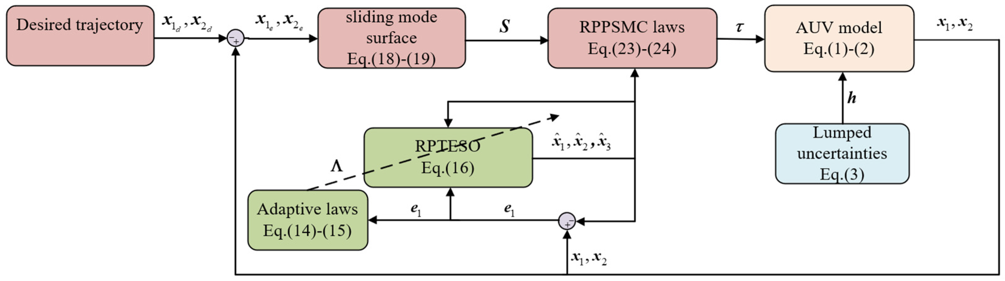
  • A new RPTESO was proposed to observe the AUV states and lumped disturbances, and its conservative upper bound of convergence time can be directly designed as only one explicit parameter, regardless of the initial state. An adaptive law was proposed to effectively enhance the robustness of the observer.
  • Considering the dynamic and kinematic characteristics of AUV, a new RPPSMC method was proposed. Additionally, it was proven that the sliding mode surface and the RPPSMC is predefined-time stable. A new control scheme with strong robustness was designed in combination with RPTESO.
  • Compared with some existing AUV trajectory-tracking control systems such as those that are based on finite-time and fixed-time theories, the proposed control scheme does not require a complicated parameter adjustment process and can flexibly adjust the convergence time of the system according to the actual requirements.
The remainder of this paper is organized as follows. In Section 2, some prior knowledge required in this study is introduced, and the AUV numerical model is provided along with the control target. In Section 3, an RPTESO and an RPPSMC are proposed. In Section 4, the stability of the control system is analyzed. In Section 5, numerical simulations and comparative experiments are presented to verify the effectiveness and superiority of the proposed method. The final section summarizes the study.
Notations 1.
In brief,  λ min ( )  is the minimum eigenvalue of the matrix  ( ) . λ max ( )  is the maximum eigenvalue of matrix  ( ) . I n n × n  denotes the nth order identity matrix.  x α x α s i g n ( x )  with  α > 0  and  x . s i g n ( x )  is a signum function.

2. Preliminaries and Problem Formulation

2.1. AUV Mathematical Model

In this section, the hydrodynamic model of a benthic AUV is analyzed [31]. The coordinate system, as shown in Figure 1, is the earth-fixed coordinate system ( E x E y E z E ) and body-fixed coordinate system ( O x B y B z B ). η = x , y , z , ϕ , θ , ψ T denotes the position and attitude in E x E y E z E , v = u , v , w , p , q , r T denotes the velocities in O x B y B z B . Based on the abovementioned definitions, the kinematic and kinetic equations can be expressed as follows:
η ˙ = J η v ,
M v ˙ + C v v + D v v + g η = τ + τ E ,
In Equation (2), M = M ¯ + M ˜ , C v = C ¯ v + C ˜ v , D v = D ¯ v + D ˜ v and g η = g ¯ η + g ˜ η . M ¯ , C ¯ v , D ¯ v and g ¯ η are nominal parametric terms, whereas M ˜ , C ˜ v , D ˜ v and g ˜ η are uncertain terms. τ E is the external disturbance. f is the lumped uncertainty which is defined as f = M ˜ v ˙ C ˜ v v D ˜ v v g ˜ η + τ E . Equation (2) can be rewritten as follows:
M ¯ v ˙ + C ¯ v v + D ¯ v v + g ¯ η = τ + f ,
More details of Equations (1) and (2) can be referred in [31].
Remark 1.
In the common AUV at present, the recovery moment in the roll is large, and it is difficult to make it change greatly in the marine environment, so this paper ignores the roll motion. The vectors related to AUV state contain other five degrees of freedom.

2.2. Preliminaries

Lemma 1
([20]). For system  x ˙ = f ( x , t ) , if the origin of the system is globally uniformly asymptotically stable and there exists a bounded function  T : m + 0  satisfying  x ( t , x 0 ) = 0  when  t T ( x 0 ) , if the constant  T  can be prescribed, the system can converge in prescribed time  T .
Lemma 2
([32]). For system  x ˙ = f ( x , t ) , there exists a Lyapunov function  V ( x ) : n + U 0  satisfying  V ( 0 ) = 0  and  V ( x ) > 0 ( x 0 ) . If the derivative of  V ( x )  satisfies
V ˙ π T C ϒ ( V 1   1 ϒ 2 + V 1   1 + ϒ 2 ) + Γ ,
where  T C  is the predefined time.  0 < ϒ < 1 , 0 Γ <  are the constants. The system is called predefined-time stable.
Lemma 3
([33]). For any  c > 0  and  x i 0 ,
i = 1 N x i c ( i = 1 N x i ) c , 0 < c 1 N 1 c ( i = 1 N x i ) c , c > 1 ,
Lemma 4
([29]). For any  c > 0 , if positive numbers  x 1  and  x 2  satisfy  x 1 > 2 x 2  there exists
x 1 c x 2 c ( x 1   x 2   ) c , c > 1 ( 2 c 1 ) ( x 1   x 2   ) c , 0 < c < 1 .

2.3. Control Objective

Considering the AUV numerical model, an RPTESO is proposed, which makes the observation tracking error dynamics satisfy the prescribed-time stability expressed under model uncertainty and external unknown disturbance. Additionally, we propose an RPPSMC based on RPTESO whose tracking error can provide coverage to zero within a predefined time.

3. Main Results

To realize fast tracking of the desired trajectory of the AUV under model perturbation and environmental disturbance, the main results of this study were divided into two parts. First, an RPTESO was designed, and then an RPPSMC was designed based on the observed state variables. The control framework is illustrated in Figure 2.

3.1. Design of RPTESO

Equation (3) suggests that the lumped uncertainty f will affect the accuracy of the AUV trajectory-tracking control and it cannot be accurately measured. Therefore, a new RPTESO was designed to observe f , and an adaptive law was designed to enhance the robustness of RPTESO.
Assumption 1.
The control input of AUV and its time derivative are bounded.
Assumption 2.
The lumped uncertainty  f  satisfies  f f max ,  f max  is a positive constant.
Remark 2.
The control input of AUV is mainly provided by two parts, the environmental disturbance and actuator. Because the energy of the marine environment is limited and the energy output of the AUV actuator is also limited, the control input of the AUV is bounded. The unknown lumped uncertainty  f  includes two parts: model uncertainty and external disturbance. The model term is related to the velocity, because the  v  and  v ˙  are bounded, so the model uncertainty is bounded. Hence, Assumption 1 and 2 are reasonable. In the common AUV at present, the recovery moment in the roll is large, and it is difficult to make it change greatly in the marine environment, so this paper ignores the roll motion.
To facilitate the following theoretical derivation, we define x 1 = η and x 2 = η ˙ , and the AUV numerical models Equations (1)–(3) can be rewritten as
x ˙ 1 = x 2 x ˙ 2 = N ( x 1 , x 2 ) + J ( x 1 ) M ¯ 1 τ + Δ ,
where
N ( x 1 , x 2 ) = J ˙ ( x 1 ) J 1 x 2 + J ( x 1 ) M ¯ 1 ( C ¯ x 2 x 2 + D ¯ x 2 x 2 + g ¯ x 1 ) ,
Δ = J ( x 1 ) M ¯ 1 τ E ,
where unknown f = N ( x 1 , x 2 ) + Δ . We define x 3 = f ; then, model Equation (7) can be rewritten as
x ˙ 1 = x 2 x ˙ 2 = x 3 + J ( x 1 ) M ¯ 1 τ x ˙ 3 = f ˙ ,
To ensure the high convergence performance of ESO, we designed a monotonically increasing function
Ξ ( t ) = csc 2 ( π 2 π t 2 t f ) ,
where t is the system time. t f denotes the desired convergence time prescribed by the designer. Ξ ( t ) satisfies Ξ ( 0 ) = 1 and Ξ ( t f ) = + .
x ^ i ( i = 1 , 2 , 3 ) is defined as the estimation value of x i ( i = 1 , 2 , 3 ) . Then, the estimation error is defined as e 1 = x 1 x ^ 1 , e 2 = x 2 x ^ 2 , and e 3 = x 3 x ^ 3 . The structure of PTESO for the system Equation (10) can be constructed as
x ^ ˙ 1 = x ^ 2 + l Ξ ( t ) g 1 e 1 + ( 1 l ) k 1 Κ 1 3 e 1 2 3 x ^ ˙ 2 = x ^ 3 + J ( x 1 ) M ¯ 1 τ + l Ξ 2 ( t ) g 2 e 1 + ( 1 l ) k 2 Κ 2 3 e 1 1 3 x ^ ˙ 3 = l Ξ 3 ( t ) g 3 e 1 + ( 1 l ) k 3 Κ e 1 0 ,
where Κ is a Lipschitz constant satisfying Κ > f max , k 1 = 3.34 k 3   1 3 , k 2 = 5.3 k 3   2 3 [34]. g i ( i = 1 , 2 , 3 ) are the positive coefficient. l is the time switch function defined as
l = 1 , t 0 , t f 0 , t t f , + ,
In the prescribed-time interval t 0 , t f , the observer is guaranteed to converge using the function Ξ ( t ) . Then, the PTESO can maintain the error at the origin in t t f , +  [34].
However, the marine environment is complex and changeable. To improve the robustness of PTESO, an adaptive law Λ = diag Λ 1 Λ 5 is proposed based on e 1 . First, Λ can be regarded as a gain coefficient. Λ should be designed as a positive term that always increases, so as to ensure an effective convergence coefficient, and at the same time, A should not be too large, otherwise it may lead to excessive overshoot and ultimately affect the observer estimation effect. Λ  is defined as
Λ ˙ = ϖ e ,
ϖ e = e 1 Θ sat ( Θ e 1 ) ,
where Θ is a positive gain coefficient. Subsequently, Equation (12) can be revised to obtain RPTESO, which is designed as
x ^ ˙ 1 = x ^ 2 + l ( Λ Ξ ( t ) g 1 e 1 + Λ 1 Λ ˙ e 1 ) + ( 1 l ) k 1 Κ 1 3 e 1 2 3 ) x ^ ˙ 2 = x ^ 3 + J ( x 1 ) M ¯ 1 τ + l Λ 2 Ξ 2 ( t ) g 2 e 1 + ( 1 l ) k 2 Κ 2 3 e 1 1 3 x ^ ˙ 3 = l Λ 3 Ξ 3 ( t ) g 3 e 1 + ( 1 l ) k 3 Κ e 1 0 ,

3.2. Design of a Predefined-Time Sliding Mode Control

In some AUV trajectory-tracking control projects, the tracking error must converge to the near-zero domain as soon as possible. Therefore, an RPPSMC is proposed based on the RPTESO proposed in Section 3.1, which enables the AUV to track the expected trajectory within an artificially predefined time under model uncertainties and environmental disturbances.
To track the desired trajectory of the AUV, we define the tracking error x 1   e = x 1   e 1 , x 1   e 2 , , x 1   e n as
x 1   e = x 1 x 1   d ,
where x 1   d is the desired value of x 1 , and we design the predefined-time sliding mode surface s as
s = x ˙ 1 e i + Ψ ( x 1   e i ) ,
Ψ ( x 1   e i ) = π T 1 μ 1 ( ( 1 2 ) 1 μ 1 2 x 1   e i 1 μ 1 + n μ 1 2 ( 1 2 ) 1 + μ 1 2 x 1   e i 1 + μ 1 ) + x 1   e i i = 1 , 2 , , n ,
The time derivative of Ψ ( x 1   e ) is defined as Ψ ˙ ( x 1   e , x ˙ 1 e ) , satisfying
Ψ ˙ ( x 1   e , x ˙ 1 e ) = π x ˙ 1 e 2 T 1 μ 1 ( ( 1 μ 1 2 ) x 1   e μ 1 2 + n μ 1 2 ( 1 2 + μ 1 4 ) x 1   e μ 1 2 ) + x ˙ 1 e ,
where T 1 is the predefined time and μ 1 > 0 is a positive constant.
Theorem 1.
For a positive constant  ϑ . If  s 2 ϑ , the  s  is predefined-time stable.
Proof of Theorem 1.
When s 2 ϑ , we chose the Lyapunov function as
V = 1 2 x 1   e T x 1   e ,
Then, taking the time derivative of Equation (21) and invoking Lemma 3, we obtain
V ˙ = x 1   e T ( s Ψ ( x 1   e ) ) = x 1   e T s x 1   e T π T 1 μ 1 ( ( 1 2 ) 1 μ 1 2 x 1   e i 1 μ 1 + n μ 1 2 ( 1 2 ) 1 + μ 1 2 x 1   e i 1 + μ 1 ) x 1   e T x 1   e x 1   e T π T 1 μ 1 ( ( 1 2 ) 1 μ 1 2 x 1   e i 1 μ 1 + n μ 1 2 ( 1 2 ) 1 + μ 1 2 x 1   e i 1 + μ 1 ) x 1   e T x 1   e + x 1   e T x 1   e + 1 4 s T s π T 1 μ 1 ( V 1   1 μ 1 2 + V 1   1 + μ 1 2 ) + 1 4 ϑ ,
By applying Equation (22) and Lemma 2, the tracking error η e converges to the sliding-mode surface within the bounds of a predefined time T 1 .
Based on the predefined-time sliding mode surface Equation (18), RPPSMC can be designed as follows
τ = M J 1 ( x ^ 3 Ψ ˙ + Π + x ¨ 1 d ) ,
Π = π T 2 μ 2 ( ( 1 2 ) 1 μ 2 2 sig 1 μ 2 ( s ) + n μ 2 2 ( 1 2 ) 1 + μ 2 2 sig 1 + μ 2 ( s ) ) 1 2 s ,
where T 2 is the predefined time and μ 2 > 0 is a positive constant. □

4. Stability Analysis

Theorem 2.
For system Equation (10) with the designed RPTESO Equation (16), the state of the estimation error model can converge in  t 0 , t f  and it can maintain at the origin in  t t f , + .
Proof of Theorem 2.
In t 0 , t f . According to Equations (12)–(16), the estimation dynamic error is obtained as
e ˙ 1 = e 2 l Λ Ξ g 1 e 1 l Λ 1 Λ ˙ e 1 ( 1 l ) k 1 Κ 1 3 e 1 2 3 e ˙ 2 = e 3 l Λ 2 Ξ 2 g 2 e 1 ( 1 l ) k 2 Κ 2 3 e 1 1 3 e ˙ 3 = f ˙ l Λ 3 Ξ 3 g 3 e 1 ( 1 l ) k 1 Κ e 1 0 ,
For the convenience of subsequent calculations, we define the alternative errors as e ^ 1 = Λ e 1 , e ^ 2 = e 2 , and  e ^ 3 = Λ 1 e 3 . Because Λ is clearly bounded, then e i = 0 is satisfied when e ^ i = 0 for i = 1 , 2 , 3 . Therefore, Equation (25) can be rewritten as
e ^ ˙ 1 = Λ e ^ 2 Ξ Λ g 1 e ^ 1 e ^ ˙ 2 = Λ e ^ 3 Ξ 2 Λ g 2 e ^ 1 e ^ ˙ 3 = Λ 1 f ˙ Λ 1 Λ ˙ e ^ 3 Ξ 3 Λ g 3 e ^ 1 ,
To simplify the calculation, Equation (26) can be further rewritten as
Φ ˙ = Λ A Φ Λ Β C D Φ + Ρ ,
where Φ = e ^ 1 , e ^ 2 , e ^ 3 , A = 0 1 0 0 0 1 0 0 0 , Β = diag Ξ , Ξ 2 , Ξ 3 , C = g 1 , g 2 , g 3 T D = 1 , 0 , 0 , Ρ = 0 , 0 , Λ 1 f ˙ Λ 1 Λ ˙ e ^ 3 .
Then, introducing the state transformation
Φ ˜ = Β ˜ Φ ,
where Β ˜ = diag g ˜ 2 Ξ 3 , g ˜ Ξ 2 , Ξ , g ˜ is any constant; thus, Because Ξ is a monotonically increasing function, it satisfies lim t t f Β ˜ = + . Then, taking the time derivative of Equation (28) yields
Φ ˜ ˙ = Β ˜ ˙ Φ + Β ˜ Φ ˙ = Ξ ˙ Ξ 1 Q Φ ˜ + Λ Β ˜ ( A Β C D ) Β ˜ 1 Φ ˜ + Β ˜ Ρ ,
where Q = diag 3 , 2 , 1 . Moreover, Β ˜ A Β ˜ 1 = g ˜ Ξ A and Β ˜ Β C D Β ˜ 1 = g ˜ Ξ C ˜ D , where C ˜ = g 1 g ˜ , g 2 g ˜ 2 , g 2 g ˜ 3 T . Thus, it satisfies
Φ ˜ ˙ = Ξ ˙ Ξ 1 Q Φ ˜ + Ξ Λ g ˜ ( A C ˜ D ) Φ ˜ + Β ˜ Ρ ,
We define a Lyapunov function as
V Φ ˜ = Φ ˜ T Γ Φ ˜ ,
where Γ is a positive definite symmetric matrix defined as Γ = Γ 1 Γ 2 Γ 3 Γ 4 Γ 5 Γ 6 Γ 7 Γ 8 Γ 9 .
Then, taking the time derivative of Equation (31) yields
V ˙ Φ ˜ = Φ ˜ ˙ T Γ Φ ˜ + Φ ˜ T Γ Φ ˜ ˙ = Ξ ˙ Ξ 1 Φ ˜ T Q T Γ Φ ˜ + Ξ ˙ Ξ 1 Φ ˜ T Γ Q Φ ˜ + Ξ Λ g ˜ Φ ˜ T ( A C ˜ D ) T Γ + Γ ( A C ˜ D ) Φ ˜ + P Φ ˜ T Γ Φ ˜ + Φ ˜ T Γ Φ ˜ P ,
Because Γ is a positive definite symmetric matrix, and matrices Γ , A , C ˜ , and D satisfying the linear matrix inequalities in [19] yields
( A C ˜ D ) T Γ + Γ ( A C ˜ D ) A + A T γ I n ε 1 I n Γ Q + Q Γ ε 2 I n ,
where γ can be any constant and ε 1 and ε 2 are the positive constants.
Substituting Equation (33) into Equation (32) yields
V ˙ Φ ˜ Ξ ˙ Ξ 1 Φ ˜ T Q T Γ Φ ˜ + Ξ ˙ Ξ 1 Φ ˜ T Γ Q Φ ˜ + Ξ Λ g ˜ ( A + A T γ I n ) Φ ˜ 2 + P Φ ˜ T Γ Φ ˜ + Φ ˜ T Γ Φ ˜ P ,
Additionally, we assume Λ ( 0 ) 1 , then Λ 1 . Using Young’s inequality yields
P Φ ˜ T Γ Φ ˜ + Φ ˜ T Γ Φ ˜ P Λ 1 Ξ f ˙ 2 Γ 3 , 2 Γ 5 , 2 Γ 6 Φ ˜ + Ξ Λ 1 Λ ˙ Γ max Φ ˜ 2 Ξ Γ max f max Φ ˜ + Ξ Λ 1 Λ ˙ Γ max Φ ˜ 2 σ Ξ Φ ˜ 2 + Ξ ( Γ max f max ) 2 4 σ + Ξ Λ 1 Λ ˙ Γ max Φ ˜ 2 ,
where Γ max = 2 Γ 3 , 2 Γ 5 , 2 Γ 6 denotes a bounded number. Because Λ is bounded, we can easily obtain Λ 1 Λ ˙ δ , which is a positive constant. Then, we obtain
P Φ ˜ T Γ Φ ˜ + Φ ˜ T Γ Φ ˜ P σ Ξ Φ ˜ 2 + Ξ ( Γ max f max ) 2 4 σ + Ξ δ Γ max Φ ˜ 2 .
Combining Equations (34)–(36), we further obtained
V ˙ Φ ˜ Ξ ˙ Ξ 1 ε 2 Φ ˜ 2 + Ξ Λ g ˜ ( A + A T γ I n ) Φ ˜ 2 + σ Ξ Φ ˜ 2 + Ξ ( Γ max f max ) 2 4 σ + Ξ δ Γ max Φ ˜ 2 .
Then, we define ζ = Ξ ˙ Ξ 3 ε 2 + Λ g ˜ ( 2 A γ ) Ξ 1 + σ Ξ 1 + δ Γ max Ξ 1 ; Equation (37) can be rewritten as
V ˙ Φ ˜ ζ Ξ 2 Φ ˜ 2 + Ξ ( Γ max f max ) 2 4 σ .
To ensure the convergence of Φ ˜ , it needs to satisfy ζ < 0 first. Hence, we choose γ 2 A + 1 and g ˜ ( Ξ ˙ Ξ 3 ) max ε 2 + σ Ξ 1 + δ Γ max Ξ 1 + ι . Owing to the functional characteristics of Ξ , it is easy to obtain ζ < ι . Therefore, g ˜ ( Ξ ˙ Ξ 3 ) max ε 2 + ι .
Then, Equation (38) is rewritten as
V ˙ Φ ˜ ι Ξ 2 Φ ˜ 2 + Ξ ( Γ max f max ) 2 4 σ ,
Equation (40) can be obtained by integrating Equation (39)
V Φ ˜ exp ι t 0 t Ξ 2 ( m ) d m V Φ ˜ ( t 0 ) + ( Γ max f max ) 2 4 σ t 0 t exp ι t 0 t Ξ 2 ( s ) ds Ξ 2 ( m ) d m exp ι t 0 t Ξ 2 ( m ) d m V Φ ˜ ( t 0 ) + ( Γ max f max ) 2 4 σ t 0 t exp ι t 0 t Ξ 2 ( s ) ds + t 0 m Ξ 2 ( s ) ds Ξ 2 ( m ) d m .
In Equation (40), we can obtain a further analysis that satisfies that the following inequality holds
( Γ max f max ) 2 4 σ t 0 t exp ι t 0 t Ξ 2 ( s ) ds + t 0 m Ξ 2 ( s ) ds Ξ 2 ( m ) d m = ( Γ max f max ) 2 4 σ exp ι t 0 t Ξ 2 ( s ) ds t 0 t exp ι t 0 m Ξ 2 ( s ) ds d ( t 0 m Ξ 2 ( s ) ds ) = ( Γ max f max ) 2 4 σ ι exp ι t 0 t Ξ 2 ( s ) ds exp ι t 0 m Ξ 2 ( s ) ds   t 0 t = ( Γ max f max ) 2 4 σ ι exp ι t 0 t Ξ 2 ( s ) ds ( exp ι t 0 t Ξ 2 ( s ) ds 1 ) = ( Γ max f max ) 2 4 σ ι ( 1 exp ι t 0 t Ξ 2 ( s ) ds ) ( Γ max f max ) 2 4 σ ι .
Thus, we obtain
V Φ ˜ exp ι t 0 t Ξ 2 ( m ) d m V Φ ˜ ( t 0 ) + ( Γ max f max ) 2 4 σ ι .
It can prove that V Φ ˜ ( t ) and Φ ˜ ( t ) are bounded in t 0 , t f . Furthermore,
Φ ( t ) 2 = Β ˜ 1 Φ ˜ 2 Β ˜ 1 2 Φ ˜ 2 .
According to Rayleigh’s inequalities [35], Equation (43) is rearranged as
λ min ( Γ ) Φ ˜ 2 V Φ ˜ λ max ( Γ ) Φ ˜ 2 .
Substituting Equation (44) into Equation (43) yields
Φ ( t ) 2 Β ˜ 1 2 λ min ( Γ ) ( exp ι t 0 t Ξ 2 ( m ) d m V Φ ˜ ( t 0 ) + ( Γ max f max ) 2 4 σ ι ) ,
Β ˜ satisfies Β ˜ ( 0 ) 1 = 1 and lim t t f Β ˜ ( t ) 1 = 0 . Meanwhile, in Equation (45), exp ι t 0 t Ξ 2 ( m ) d m V Φ ˜ ( t 0 ) + ( Γ max f max ) 2 4 σ ι is bounded. Thus, lim t t f Φ ( t ) = 0 is equivalent to lim t t f e i = 0 ( i = 1 , 2 , 3 ) , which implies that the estimated errors can converge in t f .
Next, considering the situation in t t f , + and the estimation dynamic error for RPTESO, Equation (25) can be rewritten as
e ˙ 1 = e 2 k 1 Κ 1 3 e 1 2 3 e ˙ 2 = e 3 k 2 Κ 2 3 e 1 1 3 e ˙ 3 = f ˙ k 3 Κ e 1 0 .
According to [34], for p 2 n 1 = 5 , if there exists a positive κ and a set of gain parameters k i ( i = 1 , 2 , 3 ) , a Lyapunov function V ϒ must exist and satisfy
V ˙ ϒ κ V ϒ   p 1 p .
The Lyapunov function is chosen as
V ϒ = j = 1 2 α j ϒ j ( θ j , θ j + 1 ) + α 3 1 p θ 3 p ,
where arbitrary α i > 0 ( i = 1 , 2 , 3 ) , r i = 4 i ( i = 1 , 2 , 3 ) , and θ 1 = e 1 K , θ 2 = e 2 k 1 K , θ 3 = e 3 k 2 K . From the abovementioned discussion and lim t t f e i = 0 ( i = 1 , 2 , 3 ) , it is easy to determine whether the V ϒ satisfies lim t t f V ϒ = 0 . According to (Cruz-Zavala and Moreno, 2018), if k 3 > K > f max , k 1 = 3.34 k 3   1 3 , and k 2 = 5.3 k 3   2 3 , then V ˙ ϒ satisfies V ˙ ϒ κ V ϒ   p 1 p 0 , which means that V ϒ holds V ϒ = 0 in t t f , + . In means that e i = 0 was maintained for the remainder of the period. According to Lemma 1, the RPTESO is prescribed-time stable. This completes the Proof of Theorem 2. □
Theorem 3.
For the AUV system Equation (7), if RPPSMC Equations (23) and (24) and RPTESO Equation (16) with suitable parameters are applied, converges to the near-zero domain within a predefined time  T 2 .
Proof of Theorem 3.
We define a Lyapunov function as
V s = 1 2 s T s .
Considering Assumption 2 and the AUV system in Equation (10), the time derivative of V s can be described as
V ˙ s = s T ( x ¨ 1 e + Ψ ˙ ( x 1   e , x ˙ 1 e ) ) = s T ( x ¨ 1 x ¨ 1 d + Ψ ˙ ) = s T ( x 3 + J ( x 1 ) M ¯ 1 τ x ¨ 1 d + Ψ ˙ ) = s T ( x 3 + ( x ^ 3 Ψ ˙ + Π + x ¨ 1 d ) x ¨ 1 d + Ψ ˙ ) = s T ( e 3 + Π ) .
Substituting Equations (23) and (24) into Equation (50), we can obtain
V ˙ s = s T Π + s T e 3 π T 2 μ 2 ( ( 1 2 ) 1 μ 2 2 s T sig 1 μ 2 ( s ) + n μ 1 2 ( 1 2 ) 1 + μ 2 2 s T sig 1 + μ 2 ( s ) ) 1 2 s T s + 1 2 ( s 2 + e 3 2 ) = π T 2 μ 2 ( ( 1 2 ) 1 μ 2 2 s T sig 1 μ 2 ( s ) + n μ 1 2 ( 1 2 ) 1 + μ 2 2 s T sig 1 + μ 2 ( s ) ) + 1 2 e 3 2 .
By applying Lemmas 3 and 4, we obtain the following:
s T s 1 μ 2 = i = 1 n s i 2 μ 2 ( i = 1 n s i 2 ) 1 + μ 2 2 = 2 1 μ 2 2 V s   1 μ 2 2 ,
s T s 1 + μ 2 = i = 1 n s i 2 + μ 2 n μ 1 2 ( i = 1 n s i 2 ) 1 + μ 2 2 = n μ 1 2 2 1 + μ 2 2 V s   1 + μ 2 2 .
Substituting Equations (52) and (53) into Equation (51) yields
V ˙ s π T 2 μ 2 ( ( 1 2 ) 1 μ 2 2 2 1 μ 2 2 V s   1 μ 2 2 + n μ 2 2 ( 1 2 ) 1 + μ 2 2 n μ 1 2 2 1 + μ 2 2 V s   1 + μ 2 2 ) + 1 2 e 3 2 = π T 2 μ 2 ( V s   1 μ 2 2 + V s   1 + μ 2 2 ) + 1 2 e 3 2 .
By applying Equation (54) and Lemma 2, the s can converge under the bounds T 2 . Theorem 3 is proved. □

5. Simulation Verification

In this section, two parts of comparative simulation experiments are described to demonstrate the effectiveness and superiority of the proposed RPPSMC and RPTESO. In the first step, RPTESO is compared with the fixed-time ESO to prove its superiority. In the second step, RPPSMC is compared with fixed-time SMC to prove that RPPSMC has better control performance. The XH-3000 benthic AUV used in the simulation was designed and manufactured by the Harbin Engineering University, and its model parameters were proposed in our previous research [36]. The simulation experiment was performed using MATLAB, and the simulation step was 0.001 s.

5.1. Comparative Verification with Fixed-Time ESO

The reference trajectory η d is described as
x d = 10 cos ( 0.1 t ) y d = 10 sin ( 0.1 t ) z d = 3 0.1 t θ d = 0 ψ d = 0.1 t + 0.5 π .
The external disturbances are set as
τ E = 15 sin ( 0.2 t ) + 5 9 sin ( 0.3 t ) + 4 10 sin ( 0.1 t ) 7 5 sin ( 0.2 t ) + 4 6 sin ( 0.1 t ) 4 .
The initial position states of the AUV were set as η 0 = [ 12 , 3 , 1 , π / 4 , 0 ] , and the velocity states were set as η ˙ 0 = [ 0 , 0 , 0 , 0 , 0 ] . The initial states of the RPTESO were set to x ^ 1 = η 0 , x ^ 2 = η ˙ 0 , and x ^ 3 = [ 0 , 0 , 0 , 0 , 0 ] . The first simulation experiment was conducted for two cases, t f = 0.3 s and t f = 0.5 s , to prove that the proposed method can flexibly accelerate the convergence speed. Next, for a fairer comparison, a fixed-time ESO was adopted for the comparison experiment, as described in Equation (57)
x ^ ˙ 1 = x ^ 2 + m 1 e 1 α 1 + n 1 e 1 β 1 x ^ ˙ 2 = x ^ 3 + J ( x 1 ) M ¯ 1 τ + m 2 e 1 α 2 + n 2 e 1 β 2 x ^ ˙ 3 = m 3 e 1 α 3 + n 3 e 1 β 3 .
The controller adopted a fixed-time SMC [37]. The details of the comparison method are as follows:
τ = ξ ( s ) ( α 4 s i g ( s ) ε 5 + β 4 s i g ( s ) λ 4 ) k 5 + x ¨ 1 d z 3 + ϒ ˙ s = x ˙ 1 e + ϒ ϒ = ξ ( x 1 e ) ( α 4 s i g ( x 1 e ) ε 4 + β 4 s i g ( x 1 e ) λ 4 ) k 5 ε 4 = 1 2 p 4 + 1 2 q 4 + ( 1 2 q 4 1 2 p 4 ) sgn ( x 1 e 1 ) λ 4 = 1 2 k 4 + 1 2 q 4 + ( 1 2 q 4 1 2 k 4 ) sgn ( x 1 e 1 ) ξ ( x 1 e ) = a 4 + ( 1 a 4 ) exp ( b 4 x ¯ 1 ) c 4 ε 5 = 1 2 p 5 + 1 2 q 5 + ( 1 2 q 5 1 2 p 5 ) sgn ( s 1 ) λ 5 = 1 2 k 5 + 1 2 q 5 + ( 1 2 q 5 1 2 k 5 ) sgn ( s 1 ) ξ ( s ) = a 5 + ( 1 a 5 ) exp ( b 5 s ¯ ) c 5 .
Because the comparison method was different from the model parameters adopted in this study, the parameters were readjusted to obtain improved simulation results before a comparison was made to ensure the fairness of the comparison experiment. The initial states of the fixed-time ESO were the same as those of RPTESO. The parameters of the RPTESO, fixed-time ESO, and fixed-time SMC are listed in Table 1.
A trajectory-tracking simulation experiment was conducted without disturbance to verify the effectiveness of the controller in [37]. As shown in Figure 3, the controller ensures that the AUV converges to the desired trajectory. Figure 4, Figure 5 and Figure 6 represent the estimation error results for the system states using different observers. It can be observed from Figure 4, Figure 5 and Figure 6 that all three controllers can cause the observation error to converge to the near-zero domain in a short time. Compared with the fixed-time ESO, the RPTESO has a smaller observation peak and faster convergence speed. This is because the fixed-time ESO only can obtain a relatively optimal result by adjusting the other parameters of the observer.
The convergence time of the RPTESO can be designed as an explicit parameter, and the upper bound of the observer convergence time can be set by the value of t f . The partial enlargement of Figure 4, Figure 5 and Figure 6 proves that the actual convergence time of the RPTESO is very close to the values t f = 0.3 s and t f = 0.5 s . To further quantify the observer performance of lumped uncertainties, the values of the integral absolute error (IAE) and integral time-weighted absolute error (ITAE) of e 3 are listed in Table 2. As observed from Table 2, IAE and IATE with t f = 0.3 are smaller than the observer with t f = 0.5 . This is because smaller t f leads to a faster convergence speed. However, this is due to the lag of lumped uncertainty observer estimation, which leads to a large overshoot peak in the initial stage of observation, which shows that t f = 0.5 is only reduced in e 31 , and even greatly improved in the other four degrees of freedom which shows that RPTESO has a worse transient performance. However, in the results of ITAE, the average sum of ITAE of RPTESO is smaller than that of the fixed-time ESO, which shows that RPPESO has better global steady-state performance and a higher overall estimation accuracy. Therefore, as a whole, it can be concluded that the designed RPTESO has a better state estimation performance.
In order to illustrate the control performance of the designed adaptive law, the RPTESO with t f = 0.5 and the nonadaptive ESO are compared in further simulation experiments. Figure 7 shows the curve of the observation error e 3 over time. Because the initial error and the value of Ξ ( t ) were small, the observation performances of the two methods were almost the same. With increasing time, the adaptive law can be rapidly increased to improve the convergence speed. In Figure 8, when time approaches t f , because the value of Ξ ( t ) is already large, the value of the adaptive law increases slowly to avoid overshoot, whereas the nonadaptive ESO can converge to zero more quickly because of the use of a large fixed-value coefficient, but there is an obvious overshoot. Therefore, the adaptive law designed in this study improves the robustness of the observer.

5.2. Comparative Verification with Fixed-Time SMC

To verify the control performance of the RPPSMC, two RPPSMCs with different and fixed-time SMC were compared. Simultaneously, to further illustrate the advantages of the ESO in dealing with lumped uncertainties, additional simulation experiments were performed without compensation from the ESO. The change rate of the AUV’s external disturbance can be improved as follows:
τ E = 15 sin ( 0.6 t ) + 5 9 sin ( 0.9 t ) + 4 10 sin ( 0.3 t ) 7 5 sin ( 0.6 t ) + 4 6 sin ( 0.3 t ) 4 ,
The parameters of the reference trajectory, initial AUV state, and fixed-time SMC are the same as those in Section 5.1. The parameters of the two RPPSMC methods proposed in this study are listed in Table 3.
Figure 9 shows the trajectory-tracking results for the desired trajectory. It shows that all four methods successfully completed the effective tracking of the desired trajectory even under a worse environment. The local enlarged figure shows that the two RPPSMCs proposed in this study can converge to the desired trajectory faster than the two fixed-time SMCs. This means that the RPPSMC has a better control performance.
The position and attitude tracking errors in Figure 10 further confirm similar conclusions in Figure 9. IAE and IAME in Table 4 show that the RPPSMC-1 has a better tracking performance and steady-state performance than the fixed-time SMC. However, some results of the IAE and IATE of the RPPSMC-2 are bigger than the fixed-time SMC. This is because the predefined-time T of RPPSMC-2 is set as larger, leading to a longer actual rising time, so the value of T cannot be set too large.
It can be observed from Figure 9, Figure 10 and Figure 11 that the controller without ESO compensation has a slower convergence speed and lower accuracy when tracking the trajectory. Even in the later stages of control, when the other three methods ensured a stable tracking state, oscillations still occurred. This is because the controller can only calculate the corresponding control input according to the current state error but cannot reduce the adverse effects of lumped uncertainties. When a disturbance affects the state of the AUV, the controller cannot respond in time. Therefore, it cannot stably fit the expected trajectory at all times. This implies that it is necessary to design an ESO to observe lumped uncertainties. The control inputs for the four methods are shown in Figure 12. As shown in the figure, all the control inputs were bounded and within the power range provided by the AUV. Compared with the initial control input of the fixed-time SMC, the input of the RPPSMC is larger, and a smaller predefined time T leads to a larger initial control input because it is necessary to ensure a faster convergence speed. This also explains why the velocity-tracking error of the RPPSMC in Figure 11 has a larger peak. Although the control input changes sharply in the initial stage, it decreases rapidly and tends to stabilize after the tracking error converges to a small value, which not only ensures convergence speed but also enables the AUV to enter a relatively stable state as soon as possible. Particularly, the two different RPPSMCs in Figure 9, Figure 10 and Figure 11 show something in common: (1) the system converges within a set predefined time T ; and (2) when a shorter predefined time T was set, the system converged faster, and the convergence time varied with the given predefined time T . Compared with the unknown convergence time of the fixed-time SMC, the RPPSMC can set the upper bound of the convergence time more flexibly by adjusting the explicit parameter T .

6. Conclusions

In this study, a predefined-time SMC based on a prescribed-time ESO is proposed for an AUV trajectory-tracking control. First, to reduce the adverse effects of lumped uncertainties on the trajectory-tracking control, an RPTESO is designed, and the upper bound of the observation convergence time can be directly designed as an explicit parameter instead of relying on the initial conditions or various parameter adjustments. To improve the robustness of the ESO, an adaptive law is designed to ensure that the observer has a fast convergence speed and can avoid an excessive overshoot. Second, considering the requirements of the AUV’s hydrodynamic design and rapid convergence of the trajectory-tracking deviation, an RPPSMC is designed, and the upper bound of the total convergence time T can also be directly set as an explicit parameter. A stability theory analysis proved that the sliding surface and controller meet the predefined-time convergence characteristics. Finally, the effectiveness and superiority of the proposed algorithm are verified through simulation experiments.

Author Contributions

Conceptualization, Y.X.; methodology, Y.X.; software, Y.X. and Z.Z.; validation, Y.X.; writing—original draft preparation, Y.X.; writing—review and editing, Z.Z. and L.W. All authors have read and agreed to the published version of the manuscript.

Funding

This work is supported by the National Natural Science Foundation of China (51939003).

Institutional Review Board Statement

Not applicable.

Informed Consent Statement

Not applicable.

Data Availability Statement

The original contributions presented in the study are included in the article, further inquiries can be directed to the corresponding authors.

Conflicts of Interest

The authors declare no conflict of interest.

References

  1. Zhang, Z.; Xu, Y.; Wan, L.; Chen, G.; Cao, Y. Rotation matrix-based finite-time trajectory tracking control of AUV with output constraints and input quantization. Ocean. Eng. 2024, 293, 116570. [Google Scholar] [CrossRef]
  2. Chen, G.F.; Wan, L.; Jiang, C.M.; Zhang, Y.; Liu, Y.; Zhang, Z.; Xu, Y. Dynamic event-triggered observer-based control for autonomous underwater vehicles in the Trans-Atlantic Geotraverse hydrothermal field using rotation matrices. Ocean. Eng. 2023, 281, 114961. [Google Scholar] [CrossRef]
  3. Li, J.; Du, J.L.; Sun, Y.Q.; Lewis, F.L. Robust adaptive trajectory tracking control of underactuated autonomous underwater vehicles with prescribed performance. Int. J. Robust Nonlinear Control 2019, 29, 4629–4643. [Google Scholar] [CrossRef]
  4. Li, D.L.; Du, L. AUV Trajectory Tracking Models and Control Strategies: A Review. J. Mar. Sci. Eng. 2021, 9, 1020. [Google Scholar] [CrossRef]
  5. Yan, Z.P.; Zhang, C.; Tian, W.D.; Cai, S.; Zhao, L. Distributed observer-based formation trajectory tracking method of leader-following multi-AUV system. Ocean. Eng. 2022, 260, 112019. [Google Scholar] [CrossRef]
  6. Klein, I.; Gutnik, Y.; Lipman, Y. Estimating DVL Velocity in Complete Beam Measurement Outage Scenarios. IEEE Sens. J. 2022, 22, 20730–20737. [Google Scholar] [CrossRef]
  7. Jia, K.K.; Xu, W.J.; Ma, L. Correction of velocity estimation bias caused by phase-shift beamforming in acoustic Doppler velocity logs. IET Radar Sonar Navig. 2024. [Google Scholar] [CrossRef]
  8. Hou, C.; Li, X.G.; Wang, H.B.; Zhai, P.; Lu, H. Fuzzy linear extended states observer-based iteration learning fault-tolerant control for autonomous underwater vehicle trajectory-tracking system. IET Control Theory Appl. 2023, 17, 270–283. [Google Scholar] [CrossRef]
  9. Huang, F.; Xu, J.; Yin, L.A.; Wu, D.; Cui, Y.; Yan, Z.; Chen, T. A general motion control architecture for an autonomous underwater vehicle with actuator faults and unknown disturbances through deep reinforcement learning. Ocean. Eng. 2022, 263, 112424. [Google Scholar] [CrossRef]
  10. Yang, Y.; Tan, J.; Yue, D.; Xie, X.; Yue, W. Observer-Based Containment Control for a Class of Nonlinear Multiagent Systems with Uncertainties. IEEE Trans. Syst. Man Cybern. Syst. 2018, 51, 588–600. [Google Scholar] [CrossRef]
  11. Liu, P.; Xue, W.; Chen, S.; Huang, Y.; Sun, Z. An integrated solution to ACMM problem of spacecraft with inertia uncertainty. Int. J. Robust Nonlinear Control 2018, 28, 5575–5589. [Google Scholar] [CrossRef]
  12. Liu, X.; Qiu, L.; Wu, W.J.; Ma, J.; Wang, D.; Peng, Z.; Fang, Y. Finite-time ESO-based cascade-free FCS-MPC for NNPC converter. Int. J. Electr. Power Energy Syst. 2023, 148, 108939. [Google Scholar] [CrossRef]
  13. Gao, C.Y.; Dai, J.; Li, J.; Li, J.X. Finite-Time Convergence ESO-Based Nonsingular Fast Terminal Sliding Mode Control for PMSM with Unknown Parameters and Time-Varying Load. Math. Probl. Eng. 2022, 2022, 9080445. [Google Scholar] [CrossRef]
  14. Cui, L.; Jin, N.; Chang, S.P.; Zuo, Z.; Zhao, Z. Fixed-time ESO based fixed-time integral terminal sliding mode controller design for a missile. ISA Trans. 2022, 125, 237–251. [Google Scholar] [CrossRef] [PubMed]
  15. Yang, J.Y.; Li, Z.C.; Yan, H.C.; Zhang, H. Adaptive fixed-time control for nonlinear systems subject to mismatched uncertainties and external disturbance: An ESO-based strategy. Int. J. Robust Nonlinear Control 2024, 34, 3499–3515. [Google Scholar] [CrossRef]
  16. Yang, X.F.; Zhu, X.N.; Liu, W.; Ye, H.; Xue, W.; Yan, C.; Xu, W. A Hybrid Autonomous Recovery Scheme for AUV Based Dubins Path and Non-Singular Terminal Sliding Mode Control Method. IEEE Access 2022, 10, 61265–61276. [Google Scholar] [CrossRef]
  17. Zhang, L.L.; Liu, X.L.; Hua, C.C. Prescribed-Time Control for Stochastic High-Order Nonlinear Systems with Parameter Uncertainty. IEEE Trans. Circuits Syst. II-Express Briefs 2023, 70, 4083–4087. [Google Scholar] [CrossRef]
  18. Ye, H.; Song, Y. Prescribed-time Control for Linear Systems in Canonical Form Via Nonlinear Feedback. IEEE Trans. Syst. Man Cybern. Syst. 2022, 53, 1126–1135. [Google Scholar] [CrossRef]
  19. Chang, L.; Han, Q.L.; Ge, X.; Zhang, C.; Zhang, X. On Designing Distributed Prescribed Finite-Time Observers for Strict-Feedback Nonlinear Systems. IEEE Trans. Cybern. 2019, 51, 4695–4706. [Google Scholar] [CrossRef]
  20. Cui, L.; Jin, N. Prescribed-time ESO-based prescribed-time control and its application to partial IGC design. Nonlinear Dyn. 2021, 106, 491–508. [Google Scholar] [CrossRef]
  21. Zhao, J.; Cai, C.; Liu, Y. Barrier Lyapunov Function-based adaptive prescribed-time extended state observers design for unmanned surface vehicles subject to unknown disturbances. Ocean. Eng. 2023, 270, 113671–113676. [Google Scholar] [CrossRef]
  22. Zhang, W.; Wu, W.H.; Li, Z.X.; Du, X.; Yan, Z. Three-Dimensional Trajectory Tracking of AUV Based on Nonsingular Terminal Sliding Mode and Active Disturbance Rejection Decoupling Control. J. Mar. Sci. Eng. 2023, 11, 959. [Google Scholar] [CrossRef]
  23. Hu, Y.H.; Song, Z.K.; Zhang, H.C. Adaptive sliding mode control with pre-specified performance settings for AUV’s trajectory tracking. Ocean. Eng. 2023, 287, 115882. [Google Scholar] [CrossRef]
  24. Van, M.; Ge, S.S.; Ceglarek, D. Global finite-time cooperative control for multiple manipulators using integral sliding mode control. Asian J. Control 2022, 24, 2862–2876. [Google Scholar] [CrossRef]
  25. Moulay, E.; Léchappé, V.; Bernuau, E.; Plestan, F. Robust Fixed-Time Stability: Application to Sliding-Mode Control. IEEE Trans. Autom. Control 2022, 67, 1061–1066. [Google Scholar] [CrossRef]
  26. Zhou, Y.J.; Liu, J.Y.; Jiang, G.P.; Li, C. Consensus of multi-agent systems via prescribed-time sliding mode control method. Trans. Inst. Meas. Control 2022, 44, 2369–2377. [Google Scholar] [CrossRef]
  27. Sánchez-Torres, J.D.; Sanchez, E.N.; Loukianov, A.G. Predefined-time stability of dynamical systems with sliding modes. In Proceedings of the American Control Conference (ACC), Chicago, IL, USA, 1–3 July 2015. [Google Scholar]
  28. Becerra, H.M.; Vazquez, C.R.; Arechavaleta, G.; Delfin, J. Predefined-Time Convergence Control for High-Order Integrator Systems Using Time Base Generators. IEEE Trans. Control Syst. Technol. 2017, 26, 1866–1873. [Google Scholar] [CrossRef]
  29. Munoz-Vazquez, A.J.; Sanchez Torres, J.D.; Jimenez Rodriguez, E.; Loukianov, A. Predefined-Time Robust Stabilization of Robotic Manipulators. IEEE/ASME Trans. Mechatron. 2019, 24, 1033–1040. [Google Scholar] [CrossRef]
  30. Dong, F.; You, K.; Xie, L.; Hu, Q. Coordinate-free Circumnavigation of a Moving Target via a Simple PD-like Controller. IEEE Trans. Aerosp. Electron. Syst. 2020, 58, 2012–2025. [Google Scholar] [CrossRef]
  31. Xu, Y.F.; Wan, L.; Zhang, Z.Y.; Chen, G.F. Robust adaptive path following control of autonomous underwater vehicle with uncertainties and communication bandwidth limitation. Ocean. Eng. 2023, 287, 115895. [Google Scholar] [CrossRef]
  32. Xie, S.; Chen, Q. Adaptive Nonsingular Predefined-Time Control for Attitude Stabilization of Rigid Spacecrafts. IEEE Trans. Circuits Syst. II Express Briefs 2022, 69, 189–193. [Google Scholar] [CrossRef]
  33. Wang, W.C.; Hou, M.S.; Feng, D.; Liu, B.J. Predefined-time control for Euler-Lagrange systems with model uncertainties and actuator faults. Asian J. Control 2023, 25, 1591–1605. [Google Scholar] [CrossRef]
  34. Cruz-Zavala, E.; Moreno, J.A. Levant’s Arbitrary Order Exact Differentiator: A Lyapunov Approach. IEEE Trans. Autom. Control 2018, 64, 3034–3039. [Google Scholar] [CrossRef]
  35. Polyakov, A.; Fridman, L. Stability notions and Lyapunov functions for sliding mode control systems. J. Frankl. Inst. 2014, 351, 1831–1865. [Google Scholar] [CrossRef]
  36. Qin, H.; Wu, Z.; Sun, Y.; Sun, Y. Prescribed performance adaptive fault-tolerant trajectory tracking control for an ocean bottom flying node. Int. J. Adv. Robot. Syst. 2019, 16, 172988141984194. [Google Scholar] [CrossRef]
  37. Wan, L.; Zhang, D.; Sun, Y.; Qin, H.; Cao, Y.; Chen, G. Fast fixed-time vertical plane motion control of autonomous underwater gliders in shallow water. J. Frankl. Inst. 2022, 359, 10483–10509. [Google Scholar] [CrossRef]
Figure 1. Coordinate systems of XH-3000.
Jmse 12 01014 g001
Figure 2. Control framework of the proposed control system.
Jmse 12 01014 g002
Figure 3. Three-dimensional trajectory-tracking results.
Jmse 12 01014 g003
Figure 4. The result of estimation errors for position and attitude.
Jmse 12 01014 g004
Figure 5. The result of estimation errors for velocities.
Jmse 12 01014 g005
Figure 6. The result of estimation errors for lumped uncertainties.
Jmse 12 01014 g006
Figure 7. The result of estimation errors for lumped disturbance in different cases.
Jmse 12 01014 g007
Figure 8. Curves of the adaptive coefficient Λ .
Jmse 12 01014 g008
Figure 9. Three-dimensional trajectory-tracking results Λ .
Jmse 12 01014 g009
Figure 10. Time evolution of position and attitude tracking errors.
Jmse 12 01014 g010
Figure 11. Time evolution of linear and angular velocity-tracking errors.
Jmse 12 01014 g011
Figure 12. Time evolution of control inputs.
Jmse 12 01014 g012
Table 1. Parameters of comparison method.
ComponentValue
RPTSESO g 1 = 6 ,   g 2 = 8 ,   g 3 = 2 ,   K = 8 ,   k 3 = 10 ,   Θ = 10 3
Fixed-time ESO m 1 = 10 m 2 = 30 m 3 = 50 n 1 = 20 n 2 = 45 n 3 = 60 ,
α 1 = 1 α 2 = 0.9 α 3 = 0.8 β 1 = 1.2 β 2 = 1 β 3 = 0.8
Fixed-time SMC a 4 = a 5 = 1.5 b 4 = b 5 = 6 c 4 = 0.5 c 5 = 0.6 p 4 = 0.95 q 4 = 1.4 k 4 = 0.95 p 5 = 0.5 q 5 = 1 k 5 = 1.5 α 4 = β 4 = 0.3 α 5 = β 5 = 8
Table 2. IAE and ITAE of three control schemes.
Methode31e32e33e34e35
IAE = 0 T e d t RPTESO   with   t f = 0.3 2.166.389.797.2212.2
RPTESO   with   t f = 0.5 11.820.834.424.246.7
Fixed-time ESO13.97.717.6910.719
ITAE = 0 T t e d t RPTESO   with   t f = 0.3 2.062.793.152.292.66
RPTESO   with   t f = 0.5 2.63.63.322.983.8
Fixed-time ESO14.3413.6415.314.0614.24
Table 3. Parameters of comparison method controllers.
ComponentValue
RPPSMC-1 T 1 = 3.5 , T 2 = 3 , μ 1 = 0.6 , μ 2 = 0.5
RPPSMC-2 T 1 = 5.5 , T 2 = 4.5 , μ 1 = 0.6 , μ 2 = 0.5
Table 4. IAE and ITAE of three control schemes.
Method x e y e z e θ e ψ e
IAE = 0 T e d t RPPSMC-11.852.432.150.61.81
RPPSMC-22.33.122.830.72.31
Fixed-time SMC2.533.893.440.712.66
ITAE = 0 T t e d t RPPSMC-12.373.971.480.531.96
RPPSMC-26.28.38.480.543.51
Fixed-time SMC6.316.418.160.503.22
Disclaimer/Publisher’s Note: The statements, opinions and data contained in all publications are solely those of the individual author(s) and contributor(s) and not of MDPI and/or the editor(s). MDPI and/or the editor(s) disclaim responsibility for any injury to people or property resulting from any ideas, methods, instructions or products referred to in the content.

