A Computation Model for Coast Wave Motions with Multiple Breakings

Abstract

This paper presents a computational model for coast wave motions with multiple wave breakings. In the Boussinesq model, the wave breaking judgment method is combined with the wave recovery judgment condition, which stops the wave breaking process when triggered. The energy dissipation of wave breaking is corrected, and the dissipation of wave energy is maintained at about 10% during the wave recovery stage, so that the dissipation caused by the residual turbulent motion of wave breaking and the increase in wave height caused by the shallowing of waves due to the water bottom slope are offset. By comparing the calculation results with the experimental results, it is proved that this model can be used to calculate multiple wave breakings. This model is applied to discuss the influence of wave incident angle and wave period on wave height and longshore current and gives the distribution characteristics of wave height and longshore current under multiple wave breakings.

1. Introduction

During the propagation of waves from deep sea to nearshore, a series of physical phenomena such as shallowing, refraction, reflection, and wave breaking occur due to the influence of complex topography, obstacles, and currents. Currently, research on wave breaking is still in the development stage, and the specific process and underlying causes of wave breaking cannot be clearly identified. Wave breaking not only affects coastal protection but also has a significant impact on sediment movement, pollutant transport, and topographic evolution due to the wave-induced currents generated. Wave breaking occurs more than once on very gentle beaches, and after wave breaking, there is a wave recovery stage during which the wave height does not decay. As the water depth becomes shallower, waves will break again, and the above processes will occur multiple times until reaching the coast. Very gentle beaches, including those with muddy seabeds and fine sand seabeds, are very common, and the slope usually ranges from 1:100 to 1:1000 [1]. Research on multiple wave breaking calculation models has important practical significance in protecting the ecological environment, preventing coastal erosion, and repairing damaged coasts. The study of multiple wave breaking calculation models is the focus of this research.

In previous studies, two wave breaking phenomena were mostly caused by sandbar topography [2,3,4]. Baum and Basco [5] conducted a study on a longshore current under the conditions of a sandbar topography using a wave average model. The results showed that there were two wave breaking phenomena on the sandbar, and a clear bimodal distribution of longshore currents occurred on the sandbar beach. Karjadi and Nobuhisa [6] established a time-dependent quasi-three-dimensional numerical model, which was used to study wave propagation on the sandbar. The results showed that there were two wave breaking phenomena, and the wave recovery interval was relatively short. Chen et al. [7] applied the Boussinesq model to study the longshore current on sandbar topography, and the results showed that there were two wave breaking phenomena near the sandbar, and the longshore current showed a bimodal distribution, but the second peak was smaller. Elsayed et al. [8] used the X-Beach model to simulate the wave height and longshore current of fixed and mobile sandbar topographies. The numerical results reproduced the wave breaking process near the top of the sandbar in the experimental results, where two wave breaking phenomena and the wave height showed a trend of decreasing first and then increasing. The above numerical simulations were conducted on a sandbar topography as there is no impact of abrupt topography changes on gentle planar topography, making it difficult to simulate the two wave breaking numerically. In fact, there can be two or even multiple wave breakings on gentle planar topography. Shen et al. [9] observed two wave breaking phenomena in a physical model experiment on a gentle planar topography with a slope of 1:100 but did not study or discuss this phenomenon. This experiment is the focus of this study. Yan et al. [10] proposed an expression for wave energy dissipation that is suitable for multiple wave breakings in a wave average model and also provided the conditions for determining wave recovery during wave breaking. The expression for wave energy dissipation they established has the same form as the Tajima and Madsen model [11]. However, it redefines the wave energy dissipation coefficient and stabilizes the expression for the ratio of wave energy to wave height and water depth. This model is suitable for gentle topography with different slopes and can automatically calculate the occurrence of two or more wave breaking on gentle planar topography. The research results show that the wave height profile on very gentle planar topography is stepped, and the longshore current exhibits a multi-peak distribution.

This study considers the use of the Boussinesq equation to investigate multiple wave breaking phenomena, as the Boussinesq equation has been well developed and widely applied [12,13,14,15]. The Boussinesq equation considers wave breaking by adding a wave energy dissipation term to the momentum equation to deal with wave breaking [16,17,18]. It can also be reduced to a nonlinear shallow water equation with shock wave capture capability for wave breaking calculations [19,20]. Both methods judge wave breaking by comparing specific indicators with pre-specified parameters. The disadvantage of this method is that it is a long and continuous process from the beginning of wave breaking to the end of breaking, and it cannot automatically judge the recovery of waves during the wave breaking process without similar sandbar topography interference, making it impossible to stop the wave breaking process.

Inspired by the methods of Yan et al., this study considers adding the wave recovery judgment condition given by Yan et al. [10] to the Boussinesq model, allowing the Boussinesq model to also consider the occurrence of multiple wave breakings on a gentle planar topography. This study combines the wave breaking judgment method in the Boussinesq model with the wave recovery judgment condition to achieve the calculation of multiple wave breakings. The work presented in this study is as follows: First, the phenomenon of multiple wave breakings observed in the experiment by Shen et al. [9] is introduced. Then, the condition for wave recovery judgment is added to the Boussinesq model, including modifications to the wave breaking term. Next, the model is validated by comparing the calculated results with experimental results, and the model is applied to study the new characteristics of longshore currents under different conditions. Finally, the research conclusions are drawn.

2. Observation of Two Wave Breaking Phenomena in the Experiment

Shen et al. [9] conducted longshore current experiments on gentle planar topographies with slopes of 1:40 and 1:100 and observed two wave breaking phenomena in the experiment with the 1:100 slope. The multiple wave breaking calculation models proposed in this study need to be validated through the experimental results derived from the 1:100 slope. Therefore, this section introduces the longshore current experiment conducted by Shen et al. [9] with a slope of 1:100 and shows the wave conditions in which two wave breaking phenomena occurred during the experiment.

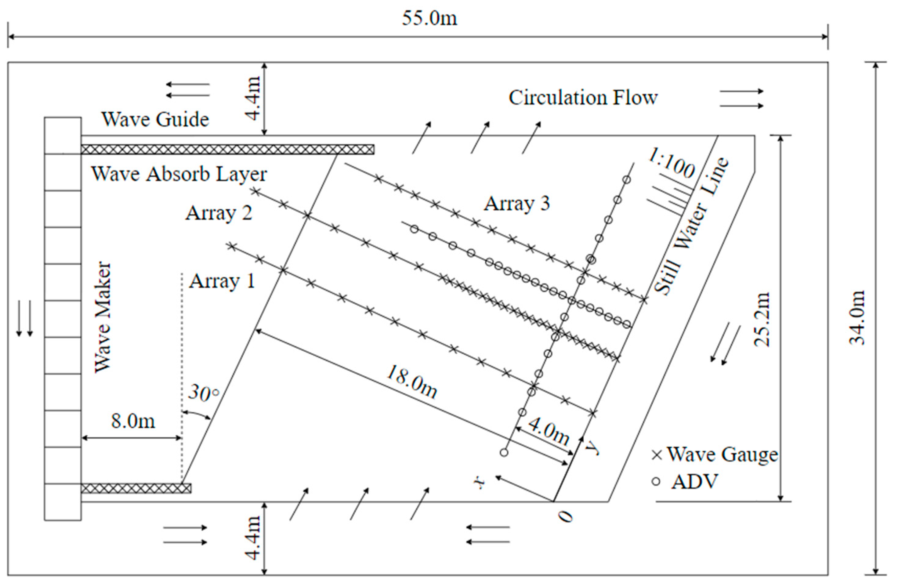
2.1. Experiment Introduction

The experiments outlined by Shen et al. [9] were carried out in the State Key Laboratory of Coastal and Offshore Engineering of Dalian University of Technology. The wave pool was 55 m long, 34 m wide, and 1.0 m deep. The topography in the experiment was at an angle of 30°. The distance between the wave maker and the foot of the slope was 8 m, the length of the topography was 18 m, and the water depth at the planar bottom was 18 cm. Waves were obliquely incident on the coastline, forming a 30° angle with the direction of incidence to generate coastal currents. The length of the waveguide walls was arranged on both sides of the wave generator, and a sponge layer was placed on the inner side of the waveguide wall to prevent wave reflection. A distance of more than 3 m above the still water line was left to provide sufficient wave climbing length. The coastal topography had a 4.4 m interval from the surrounding pool walls, and its water depth was consistent with the water depth at the planar bottom. The origin of the plane coordinate system (x, y) was at the upstream end of the still water line, with the positive x-axis pointing offshore and the positive y-axis pointing downstream. The experimental layout is shown in Figure 1.

The waves were measured through the use of three columns of capacitance-type wave gauges arranged perpendicular to the shoreline, with a spacing of 5 m per column. These were located at y = 7 m, 12 m, and 17 m. The first and third columns were mainly used as references, and the measurement results of the second column were used to compare the experimental results with the results of the numerical calculation. The measurement points of this column of wave gauges were arranged from the still water line to 10 m, with a spacing of 0.5 m, and then from 11 m to 20 m, with a spacing of 1 m. The last one was located at 22 m. The sampling rate of the wave gauges was 50 Hz. The experimental longshore current velocity was measured using acoustic Doppler velocimeters produced by Nortek. The velocimeters were arranged perpendicular to the shoreline and parallel to the shoreline, with 18 velocimeters in the direction perpendicular to the shoreline and 12 velocimeters in the direction parallel to the shoreline to measure the distribution of longshore current in the vertical shoreline direction and along the shoreline direction, respectively. In the longshore direction, the velocimeters were arranged at x = 4 m, with an interval of 2.0 m from y = 2.5 m to y = 24.5 m. In the vertical shoreline direction, the velocimeters were arranged at y = 14.5 m, with a distance from the still water line ranging from 1 m to x = 8 m with an interval of 0.5 m, followed by 9.0 m, 10.0 m, and 12.0 m. The sampling rate of velocimeters was 20 Hz, and the sampling durations were 450 s. The incident wave used in the experiment was a regular wave with three wave periods (1.0, 1.5, and 2.0 s), and each period had three wave heights. The wave conditions are shown in

Table 1. The table shows the test conditions.

Case	T (s)	H (cm)
T1H1/H2/H3	1	2.34/4.90/5.95
T1.5H1/H2/H3	1.5	2.53/4.91/5.30
T2H1/H2/H3	2	3.16/4.57/5.62

.

An average water level difference in the longshore direction formed during the experiment, resulting in circulation in the basin that was driven by the longshore current. This passive circulation system formed by the longshore current was situated in a closed harbor basin, which, when compared to an active circulation system, can only form a relatively uniform longshore current in the middle part of the beach’s topography. However, the advantage of this circulation system is that the longshore current is not affected by external artificial currents. Dalrymple [21] conducted a theoretical analysis and experimental measurements on this passive circulation system, and the results showed that a relatively uniform longshore current was formed in the middle part of the beach’s topography. Measuring a stable average longshore current distribution only requires that the longshore current be uniform in the middle part of the beach; for proof of the uniformity of longshore currents, refer to Yan et al. [10].

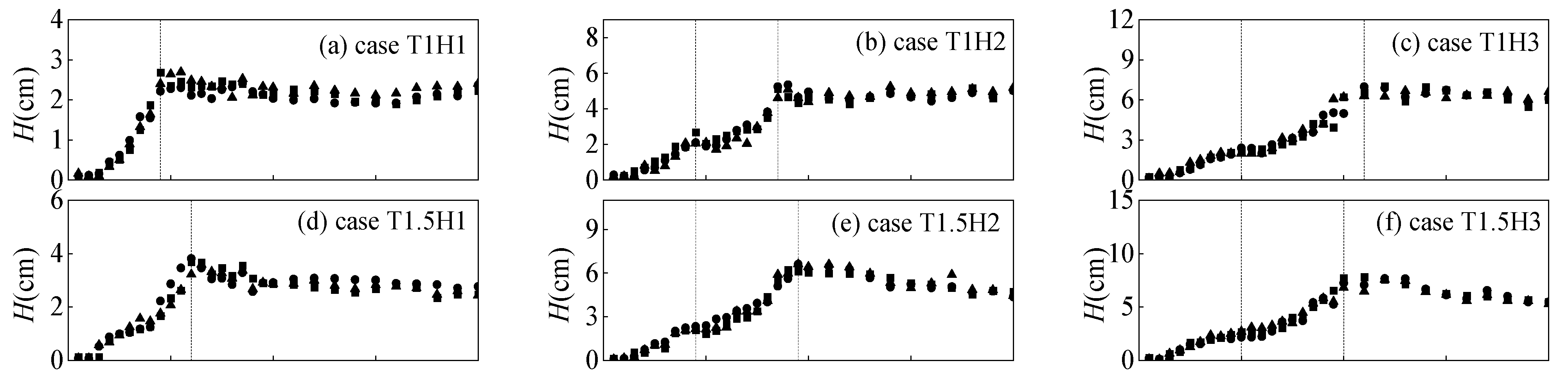
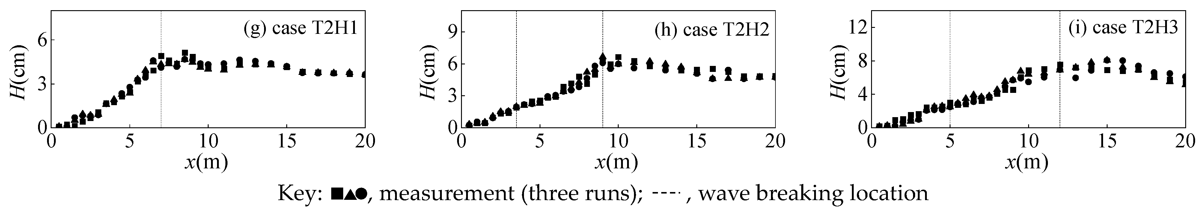
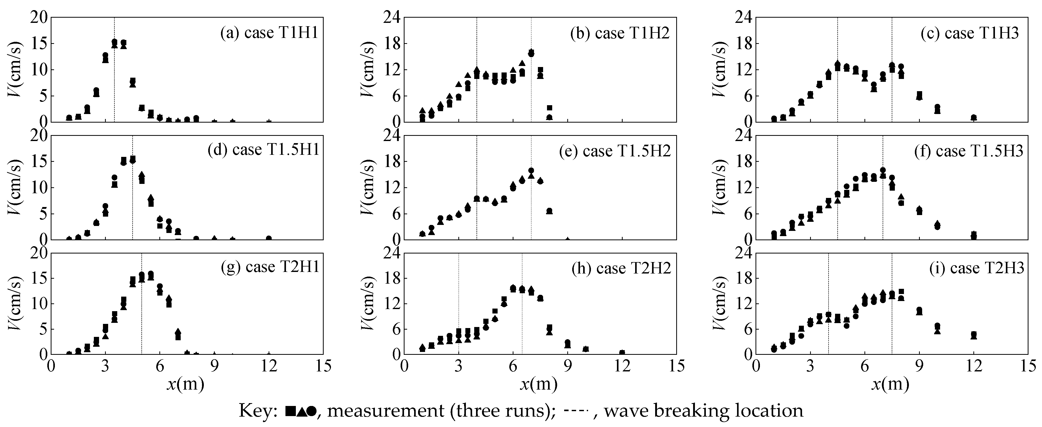
2.2. Experimental Results

This section presents the experimental results of the 1:100 slope obtained by Shen et al. [13] and points out the case of two wave breaking phenomena that appeared in the experimental results. Figure 2 shows the wave height distribution. The location of wave breaking was marked by vertical dashed lines in the figure. It can be seen from the figure that two wave breaking phenomena occurred in some cases. The wave height in these cases did not always decrease; rather, it decreased to a certain location and then remained constant until the wave broke again, and the wave height continued to decrease until reaching the coastline. Figure 3 shows the distribution of the longshore current velocity. The location of the longshore current velocity peak is marked by the vertical dashed line in the figure. It can be seen from the figure that there are two distribution shapes of longshore current velocity. When the incident wave height is small, the longshore current velocity presents an unimodal distribution. When the incident wave height is large, the longshore current velocity presents a bimodal distribution.

Shen et al. [9] did not observe two wave breaking phenomena in the 1:40 slope experiment; however, two wave breaking occurred under the 1:100 slope wave conditions.

Table 2. The experimental wave conditions with two wave breaking.

	T1H1	T1H2	T1H3	T1.5H1	T1.5H2	T1.5H3	T2H1	T2H2	T2H3
T (s)	1	1	1	1.5	1.5	1.5	2	2	2
H (cm)	2.29	4.94	5.94	2.53	4.93	5.53	3.63	4.56	5.30
Nw	1	2	2	1	2	2	1	2	2
Nv	1	2	2	1	2	2	1	2	2
SWB	No	Yes	Yes	No	Yes	Yes	No	Yes	Yes

Note: N_w = 2 indicates two wave breaking; N_v = 2 indicates longshore current with a bimodal distribution; SWB indicates two wave breaking occurring under this wave condition.

shows the experimental wave conditions with two wave breaking. In the table, N_w = 2 indicates two wave breaking, and N_v = 2 indicates that the longshore current has a bimodal distribution. SWB indicates that two wave breaking phenomena occurred under these wave conditions. The wave conditions that resulted in two wave breaking phenomena are as follows: T = 1 s, H = 4.94 cm and 5.94 cm; T = 1.5 s, H = 4.93 cm and 5.53 cm; and T = 2 s, H = 4.56 cm and 5.30 cm. It can be seen that two wave breakings occur under wave conditions with higher incident wave heights, while only one wave breaking occurs under wave conditions with lower incident wave heights. The wave conditions with two wave breaking phenomena are consistent with the wave conditions where there is a bimodal distribution of longshore current.

3. Computation Model

3.1. Governing Equation

This study uses the high-order Boussinesq equations derived by Zou and Fang [22] for the numerical simulations. The equations are as follows:

$${\eta }_t+\nabla \cdot [(h+\eta )\overline{\mathit{u}}]=0,$$

(1)

$${\overline{\mathit{u}}}_t+(\overline{\mathit{u}}\cdot \nabla )\overline{\mathit{u}}+g\nabla \eta ={\mathit{P}}^{(2)}+{\mathit{P}}^{(4)}+{\mathit{R}}_f+{\mathit{R}}_b+{\mathit{R}}_s,$$

(2)

where

$${\mathit{P}}^{(2)}={{\mathit{P}}^{\prime }}^{(2)}+{\mathit{L}}_1(\Gamma -\mathit{C}),$$

(3)

$${\mathit{P}}^{(4)}={{\mathit{P}}^{\prime }}^{(4)}-{\mathit{L}}_2\tilde{\mathit{C}},$$

(4)

$${{\mathit{P}}^{\prime }}^{(2)}=\frac{1}{2d}\nabla \{d^{2}D[\frac{2}{3}d\nabla \cdot \overline{\mathit{u}}+\nabla h\cdot \overline{\mathit{u}}]\}-\nabla hD(\frac{1}{2}d\nabla \cdot \overline{\mathit{u}}+\nabla h\cdot \overline{\mathit{u}}),$$

(5)

$$\begin{array}{l}{{\mathit{P}}^{\prime }}^{(4)}=-\frac{1}{24}{h}^3\nabla \nabla \cdot \nabla \nabla \cdot (h{\overline{\mathit{u}}}_t)+\frac{1}{12}{h}^2\nabla \nabla \cdot [h\nabla \nabla \cdot (h{\overline{\mathit{u}}}_t)]\\ +\frac{1}{120}{h}^4\nabla \nabla \cdot \nabla \nabla \cdot {\overline{\mathit{u}}}_t-\frac{1}{36}{h}^2\nabla \nabla \cdot [h^2\nabla \nabla \cdot {\overline{\mathit{u}}}_t],\end{array}$$

(6)

$${\mathit{L}}_1=({\alpha }_2-{\alpha }_1)h^2\nabla \nabla \cdot -{\alpha }_{2}h\nabla \nabla \cdot h,$$

(7)

$${\mathit{L}}_2=({\beta }_1-{\beta }_2)h^4\nabla {\nabla }^2\nabla \cdot +{\beta }_2{h}^3\nabla {\nabla }^2\nabla \cdot h,$$

(8)

$$\Gamma =\frac{1}{2}h\nabla [\nabla \cdot (h{\overline{\mathit{u}}}_t)]-\frac{1}{6}{h}^2\nabla (\nabla \cdot {\overline{\mathit{u}}}_t),$$

(9)

$$D=\frac{\partial }{\partial t}+\overline{\mathit{u}}\cdot \nabla ,$$

(10)

$$\tilde{\mathit{C}}={\overline{\mathit{u}}}_t+g\nabla \eta ,$$

(11)

$$\mathit{C}={\overline{\mathit{u}}}_t+(\overline{\mathit{u}}\cdot \nabla )\overline{\mathit{u}}+g\nabla \eta ,$$

(12)

where $\overline{\mathit{u}}$ is the average velocity of the water depth, $d=h+\eta$ is the total water depth, $\eta$ is the free surface elevation, h is the water depth, g is the acceleration of gravity, and $\nabla =(\partial /\partial x,\partial /\partial y)$ is the horizontal gradient operator. Parameter ${\alpha }_1,{\beta }_1$ is used to improve the dispersion performance of the equation, and ${\alpha }_2,{\beta }_2$ is used to improve the performance of the equation in terms of shallowing. The specific values are determined by comparing the dispersion relationship of the equation with the Stokes theory solution, which are ${\alpha }_1=1/9$, ${\beta }_1=1/945$, ${\alpha }_2=0.146488$, and ${\beta }_2=0.0019959$, respectively. Wave breaking (${\mathit{R}}_b$), subgrid turbulent mixing (${\mathit{R}}_s$), and the bottom friction (${\mathit{R}}_f$) are considered the agents of energy dissipation in the Boussinesq model. The bottom friction ${\mathit{R}}_f$ has the expression:

$${\mathit{R}}_f=\frac{f_w}{d}\overline{\mathit{u}}\left|\overline{\mathit{u}}\right|,$$

(13)

where the bottom friction coefficient $f_w$ is set to be constant, and the value range is 0.001~0.015. Subgrid turbulence mixing after wave breaking will affect the flow field of wave-induced currents, and this issue is considered through the use of this term. The subgrid lateral turbulent mixing ${\mathit{R}}_s$ can be calculated by

$$R_s^x=\frac{1}{d}\{{\nu }_s{[{(d\overline{u})}_x]}_x+\frac{1}{2}{[{\nu }_s({(d\overline{u})}_y+{(d\overline{v})}_x)]}_y\},$$

(14)

$$R_s^y=\frac{1}{d}\{{\nu }_s{[{(d\overline{v})}_y]}_y+\frac{1}{2}{[{\nu }_s({(d\overline{u})}_y+{(d\overline{v})}_x)]}_x\},$$

(15)

where superscripts x and y represent the directions in the horizontal plane, subscript $x$ and $y$ represent the spatial differentials, and ${\nu }_s$ is the eddy viscosity coefficient.

$${\nu }_s=-C_m\Delta x\Delta y{[{(\frac{\partial U}{\partial x})}^2+{(\frac{\partial V}{\partial y})}^2+\frac{1}{2}{(\frac{\partial U}{\partial y}+\frac{\partial V}{\partial x})}^2]}^{1/2},$$

(16)

where $\Delta x$ and $\Delta y$ are the grid spacing in the $x$ and $y$ directions, respectively, and $U$ and $V$ represent the time-averaged velocity, which is calculated once every two wave periods. $C_m$ is the mixing coefficient, and the value range is 0.1~2.0. The energy dissipation due to wave breaking ${\mathit{R}}_b$ has the same form of ${\mathit{R}}_s$, which reads

$$R_b^x=\frac{1}{d}\{\nu {[{(d\overline{u})}_x]}_x+\frac{1}{2}{[\nu ({(d\overline{u})}_y+{(d\overline{v})}_x)]}_y\},$$

(17)

$$R_b^y=\frac{1}{d}\{\nu {[{(d\overline{v})}_x]}_x+\frac{1}{2}{[\nu ({(d\overline{u})}_x+{(d\overline{v})}_y)]}_y\},$$

(18)

where $\nu$ is the vortex viscosity coefficient, the value of which is determined by $\nu =B{\sigma }^{2}d\left|{\eta }_t\right|$, and $\sigma$ is the breaking strength coefficient and the value range is 0.2~2.0. B controls the occurrence of wave breaking phenomenon and is defined as follows:

$$B=\left\{\begin{array}{ll}{\eta }_t/{\eta }_t^{*}-1& {\eta }_t^{*}\le {\eta }_t<2{\eta }_t^{*}\hfill \\ 1& {\eta }_t\ge 2{\eta }_t^{*}\hfill \end{array}\right.,$$

(19)

where ${\eta }_t^{*}$ is used to define the start and end times of wave breaking, i.e.,

$${\eta }_t^{*}=\left\{\begin{array}{cc}{\eta }_t^F,& t-t_0\ge T^{*},\\ {\eta }_t^I+(t-t_0)({\eta }_t^F-{\eta }_t^I)/T^{*},& 0\le t-t_0<T^{*},\end{array}\right.$$

(20)

where $T^{*}$ is the interval of wave breaking, $t_0$ is the time when wave breaking occurs, ${\eta }_t^{(I)}=e^I\sqrt{gh}$ and ${\eta }_t^{(F)}=e^F\sqrt{gh}$ are the starting and ending values of wave breaking, respectively, and $T^{*}=5\sqrt{h/g}$ is the wave breaking duration. In the Kennedy et al. [23] model, the range of $e^I$ is between 0.35 and 0.65, where 0.35 is suitable for sand bar coasts and 0.65 is suitable for gentle planar coasts.

The application of the above-mentioned wave breaking method can be used to judge two wave breaking phenomena on sand bar topographies due to the fact that wave recovery occurs on sand bar topography and no wave recovery occurs in the case of gentle planar topographies. To illustrate this point, take a 1:40 slope, T = 1.0 s, H = 9.5 cm, and h = 0.48 m as an example. Figure 4 shows the distribution of the wave height in the case of a sand bar and a gentle planar topography. It can be seen from the figure that wave recovery occurs on this sand bar topography. Figure 5 shows the time series of ${\eta }_t^{*}$ and ${\eta }_t$ at different locations. It can be seen from the figure that x = 7 m, and ${\eta }_t^{*}$ is always greater than ${\eta }_t$, meaning that the wave is unbroken at this location. At x = 5 m, ${\eta }_t^{*}$ is combined with ${\eta }_t$, meaning that the wave breaks. ${\eta }_t^{*}$ is smaller on a sandbar topography, meaning that the wave breaks more strongly on a sandbar topography. At x = 4 m and 3 m, the waves occurring on a sandbar topography experience wave recovery, while the waves that occur on a planar slope topography always break. This is reflected by the fact that ${\eta }_t^{*}$ is greater than ${\eta }_t$ on a sandbar topography, while ${\eta }_t^{*}$ and ${\eta }_t$ are combined on a planar slope topography. At x = 1 m, both the sandbar topography and planar slope topography produce breaking waves, so ${\eta }_t^{*}$ and ${\eta }_t$ are combined together. The above explanation for the above-mentioned wave breaking judgment method cannot determine two wave breaking phenomena on a planar slope topography.

In order to study the multiple wave breaking phenomenon on a planar slope topography, the wave recovery judgment condition given by Yan et al. [10] is added to the Boussinesq model, making it possible to simulate the multiple wave breaking phenomenon on a planar slope topography. This judgment condition is as follows:

$${\gamma }_r^{*}=0.28+4\tan \alpha ,$$

(21)

where $\alpha$ is the topographic inclination angle, and ${\gamma }_r^{*}$ is the ratio of wave height to water depth corresponding to wave recovery. Wave recovery is determined by comparing the relationship between the local wave height and depth ratios of $\gamma =H/h$ and ${\gamma }_r^{*}$. When $\gamma ={\gamma }_r^{*}$, it means that wave breaking stops and wave recovery begins, and the wave height no longer attenuates. Wave recovery is not initiated before wave breaking. To achieve this, it is necessary to combine the wave recovery judgment condition with the wave breaking judgment condition given above, so that the wave recovery judgment condition depends on the relationship between ${\eta }_t$ and ${\eta }_t^{*}$. When ${\eta }_t^{*}<{\eta }_t$ occurs, the wave begins to break, and the wave recovery judgment condition is also activated at the same time, comparing $\gamma$ with ${\gamma }_r^{*}$. When ${\gamma }_s^{*}<\gamma$ occurs, the wave continues to break. When ${\gamma }_r^{*}\le \gamma$ occurs, wave breaking stops. In numerical calculations, after wave breaking occurs, it is necessary to compare the relationship between $\gamma$ and ${\gamma }_s^{*}$ for each spatial step at the current time.

In order to achieve the above wave recovery in the numerical calculation model, it is necessary to modify the wave breaking term ${\mathit{R}}_b$, as follows:

$${{\mathit{R}}^{\prime }}_b={\delta }_b{\mathit{R}}_b,$$

(22)

where ${\delta }_b$ is the wave recovery control parameter. The reason for the correction of the above formula is to control the change in wave height after wave breaking. If ${\delta }_b$ = 0 is set in the wave recovery zone, it will reduce the energy dissipation of the wave, and the wave height will continue to increase and cannot remain constant. The wave height at any location has the following relationship with the wave height in deep water, $H_i=H_0{k}_s{k}_r$, where $k_s$ is the shoaling coefficient, $k_s=\sqrt{c_{g0}/c_{gi}}$, $k_r$ is the shoaling coefficient, $k_r=\sqrt{\cos {\alpha }_0/\cos {\alpha }_i}$, subscripts 0 and i represent deep water and any water depth, respectively, $c_g$ is the group velocity, $c_g=cn$, and $c$ represents the wave velocities, $n=(1+2kh/\sinh kh)/2$. As water depth decreases, $c_g$ also decreases gradually, which causes $k_s$ to increase and, thus, $H_i$ to increase. In order to maintain the wave height in the wave recovery zone, a certain amount of wave energy dissipation is required to offset the increase in wave height after the wave breaking stops. After comparison with the experimental results, ${\delta }_b$ = 0.1 is taken here. The above provides the calculation method required for considering multiple wave breakings in the Boussinesq equation.

3.2. Numerical Method and Boundary Conditions

The numerical solution of the equation is solved using the finite difference method, and the time layer is solved using the fifth-order prediction and sixth-order correction ABM (Adams–Bashforth–Moulton) format [24]. The spatial derivative in the equation is solved using the fourth-order difference format. In order to effectively avoid the influence of secondary wave reflection at the wave-making plate on the numerical results, the internal wave-making method given by Kim [25] is used, which is carried out by adding a source function to the continuity equation. In addition, a sponge absorption layer is provided at the wave-making source (left and right sides) to prevent wave reflection.

The boundary conditions used in this study include three types: (1) a solid boundary; (2) a periodic boundary, making the calculation results on both sides of the calculation domain continuous, allowing for the simulation of an infinite-length region in a finite width area; and (3) a coastal dynamic boundary, using the narrow-gap method, here refer to the approach of Chen et al. [26] and adjust the width parameter $\delta$ and shape parameter $\lambda$ of the slit to approximate the actual coast. In theory, the smaller the value of $\delta$ and the larger the value of $\lambda$, the more accurate the wave climbing simulation will be, but it will also reduce the stability of the calculation. Here, $\lambda =50$ and $\delta =0.01$ are taken. The calculation domain is shown in Figure 6.

4. Model Validation and Comparison

This section presents the two verifications of the established model: (1) validation for the judgment condition of wave recovery (21) and the modified wave breaking term (22); (2) validation of the applicability of the model to different incident wave heights. This is carried out by comparing the computational results of the present model with the experimental results. In addition, in order to illustrate the applicability of the model to different slopes, the calculation results of this model are compared with the computational results of the wave average model used by Yan et al. [10].

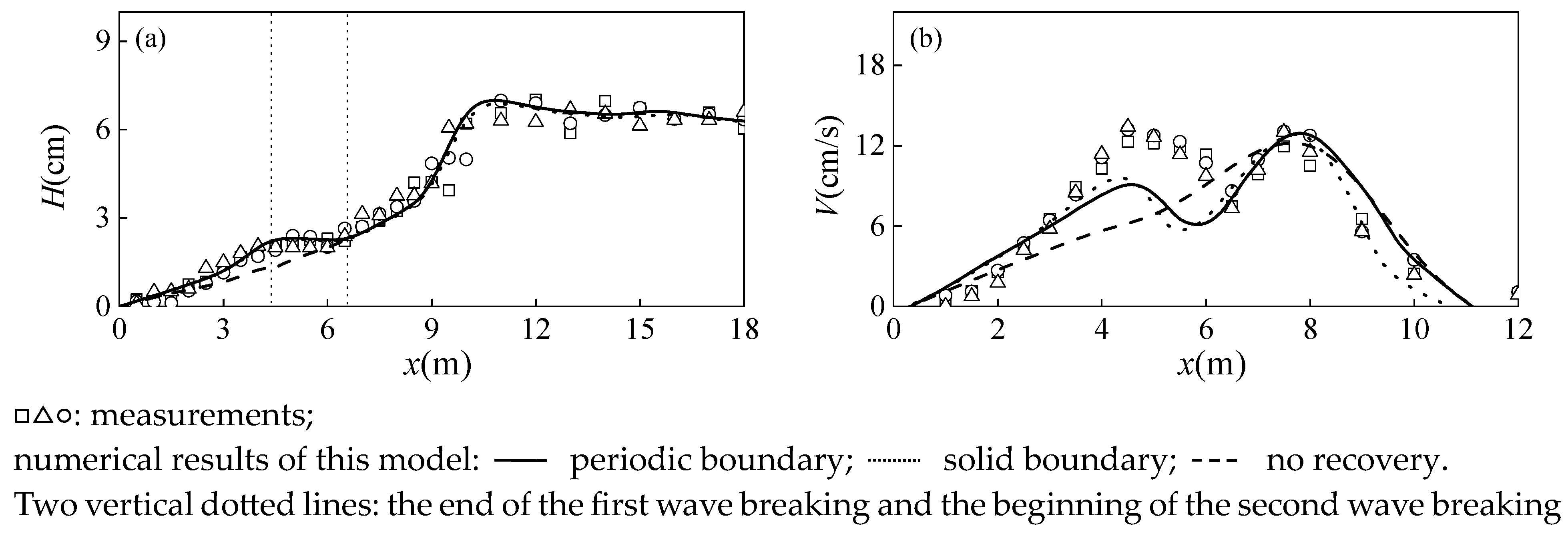
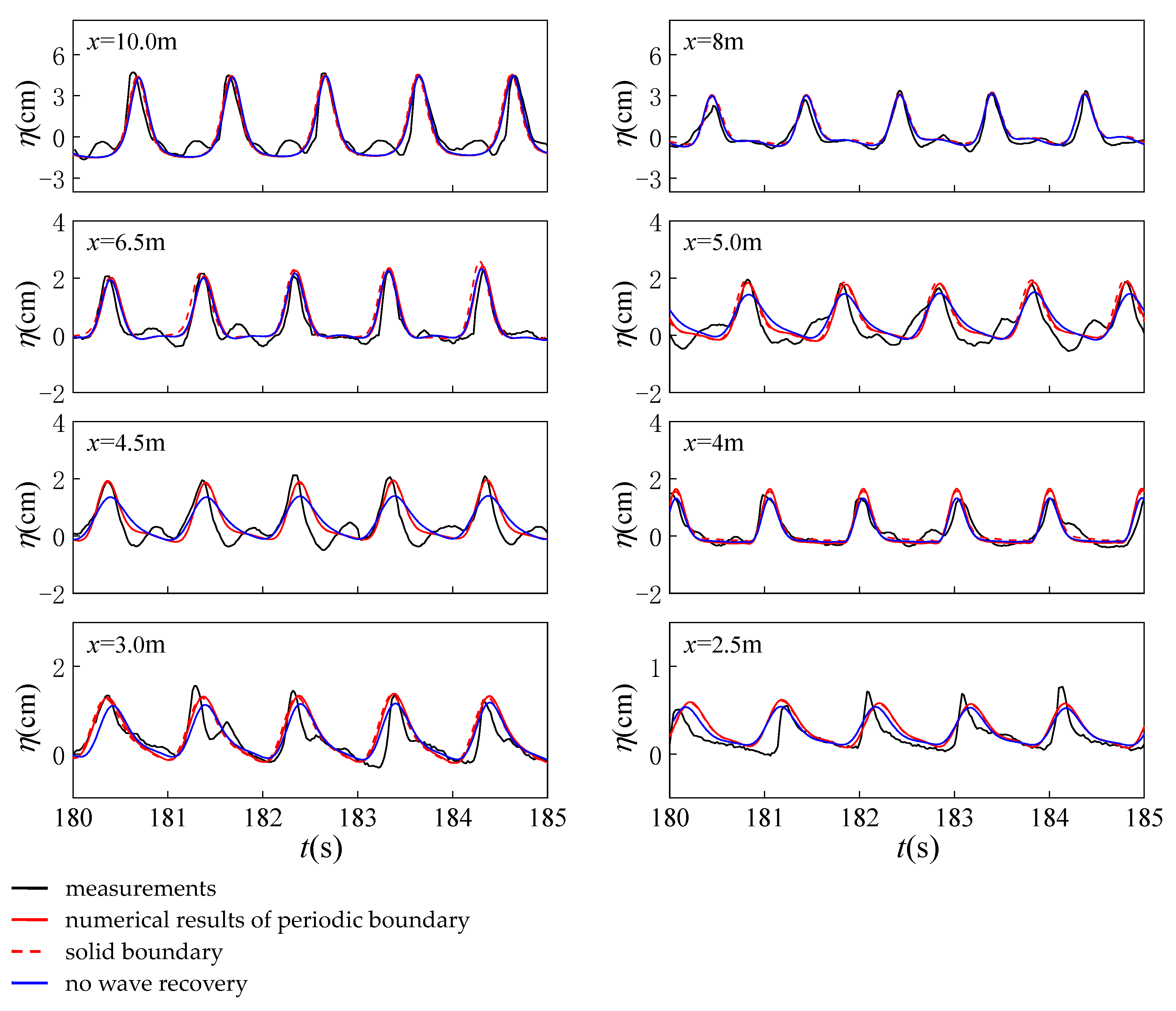
4.1. Verification for the Multiple Wave breaking Judgment condition

For comparison with the experimental results, the topography of the numerical simulation is consistent with the experimental topography, and solid boundaries are used on both sides of the coast to restore the passive circulation system formed by the longshore current in the closed harbor basin. To expand the calculation results, we also used a coastal terrain parallel to the wave maker, with periodic boundary conditions on both sides of the coast, and waves incident at an angle of 30°. This section compares the calculation results of the two boundary conditions with experimental results. The time step and space step used for numerical calculation need to satisfy the Courant stability condition, $\Delta t\le 0.5*\min (\sqrt{\Delta x^2+\Delta y^2}/\sqrt{gh})$; taking a period of 2 s as an example, the spatial and time steps are $\Delta x=0.05 \mathrm{m}$, $\Delta y=0.1 \mathrm{m}$, and $\Delta t=0.02 \mathrm{s}$, and the $\Delta t$ calculated from the Courant stability condition is 0.046 s. Therefore, the time and spatial steps used in the numerical calculations are acceptable. In the numerical simulation of the 1:100 slope experiment below, the spatial step size is $\Delta x=0.05 \mathrm{m}$ and $\Delta y=0.1 \mathrm{m}$. When the period is 1 s and 1.5 s, the time step size is $\Delta t=0.01 \mathrm{s}$, and when the period is 2 s, $\Delta t=0.02 \mathrm{s}$. By calibrating the experimental results, the parameters are set to $e^I=0.45$, $e^F=0.05$, $f_w=0.006$, $C_m=1.0$, $\sigma =1.0$.

Before comparison, it is necessary to explain the selection of the cross-section for the calculation results. Taking wave condition T2H2 as an example, Figure 7 shows the distributions of wave height and time-averaged flow field. It can be seen from the figure that the calculation results under both boundary conditions exhibit stable longshore current velocities in the middle interval. Therefore, the computational results for the location in the middle of the shoreline were chosen for comparison with the experimental results.

In order to verify the model, taking wave condition T1H3 as an example, Figure 8 shows a comparison of the wave height and longshore current velocity of different models with the experimental results. In Figure 8a, the first vertical dotted line represents the end of the first wave breaking and the beginning of the wave recovery area, and the second vertical dotted line represents the end of the wave recovery area and the beginning of the second breaking. The wave recovery area is located at x = 3.5 m–5.3 m. It can be seen from the figure that the calculation results under the two boundary conditions are consistent with the experimental results. This proves that the three contents of this model are as follows: (1) The judgment condition for the wave recovery (Equation (21)) is also suitable for the Boussinesq wave model here, which can be used to determine the location where the wave begins to recover. (2) It proves that the energy dissipation (Equation (22)) used in this model is suitable, as shown in Figure 8a. It can be seen that the wave height in the wave recovery zone tends to be constant; this is due to the dissipation of turbulence generated by wave breaking and the increase in wave height caused by wave shallowing due to the slope of the water bottom, which offset each other, resulting in a constant wave height in the wave recovery zone. (3) As shown in Figure 8, the calculation results of the first and second breaking points of waves in this model are in agreement with experimental results, indicating that Equations (19) and (20) used in this model can be used to determine the first wave breaking and determine new wave breaking occurring after the end of the wave recovery zone. The calculation results of both models are in good agreement with experimental results, and Figure 8a also shows the calculation results without wave recovery (calculated from the solid boundary), and it can be found that the wave height is continuously decaying, which is inconsistent with the experimental results. From Figure 8b, it can be seen that the distribution of longshore currents with wave recovery is bimodal, while the distribution of longshore currents without wave recovery is unimodal, which is also inconsistent with the experimental results.

In order to further verify the model, more detailed results are given for the above case. Figure 9 shows the time series of free surface elevation at different locations. It can be seen from the figure that the model can reproduce the free surface elevation in different regions, including the unbreaking region, the first breaking region, the wave recovery region, and the second breaking region, which are similar to the experimental results in terms of time series. In the unbreaking region, the time series of free surface elevation at x = 12 m and 11 m are symmetrical, while in the first breaking region, at x = 10 m and 8 m, the wave front appears asymmetric. In the recovery region, at x = 6.5 m and 5 m, the wave returns to a symmetrical state, but in the second breaking region, at x = 3.0 m and 2.5 m, a significantly asymmetric wave front appears again. This reflects the fact that the model can reproduce the free surface variation during multiple wave breaking processes, further validating the model. It can also be seen from the figure that the calculation results of the two boundary conditions are relatively consistent. To illustrate the effectiveness of wave recovery, the free surface elevation without wave recovery is also shown in Figure 9. It can be seen that at x = 5.0 m, 4.5 m, and 3 m, the free surface elevation is less than the experimental results and numerical calculation results. Although there is a certain gap between the secondary peak of the numerical results and experimental results at the trough, it can be seen from the symmetrical shape of free surface elevation in numerical results that wave recovery in this model is effective.

In order to quantitatively compare the differences between the computational results and experimental results under two boundary conditions, the error index proposed by Wilmott [27] is used for the description:

$$WIA=1-\frac{{\displaystyle \sum _{i=1}^N{\left[y(j)-x(j)\right]}^2}}{{\displaystyle \sum _{i=1}^N{\left[\left|y(j)-\overline{x}\right|+\left|x(j)-\overline{x}\right|\right]}^2}},$$

(23)

where $x(j)$ is the experimental result, $y(j)$ is the numerical result, and $\overline{x}$ is the average value of the experimental result; the larger the value of WIA, the better the agreement between the numerical value and the experimental result. When WIA = 1, it indicates that the numerical result fully agrees with the experimental result.

Table 3. The WIA values of the calculation results for the two boundary conditions.

Boundary Condition	WIA-H	WIA-V	Average
Solid	0.986	0.952	0.969
Periodic	0.984	0.913	0.948

presents the WIA values for the two boundary conditions in Figure 8. WIA-H represents the WIA value for wave height, and WIA-V represents the WIA value for coastal current velocity. It can be seen from the table that the WIA values for the solid boundary calculation results are all greater than those for the periodic boundary calculation results, but the difference between the two is relatively small, indicating that periodic boundaries can also give results that are consistent with the experiments; but the solid boundary results are more consistent with the experimental results. Therefore, in the following calculations, the solid boundary will be used for calculation.

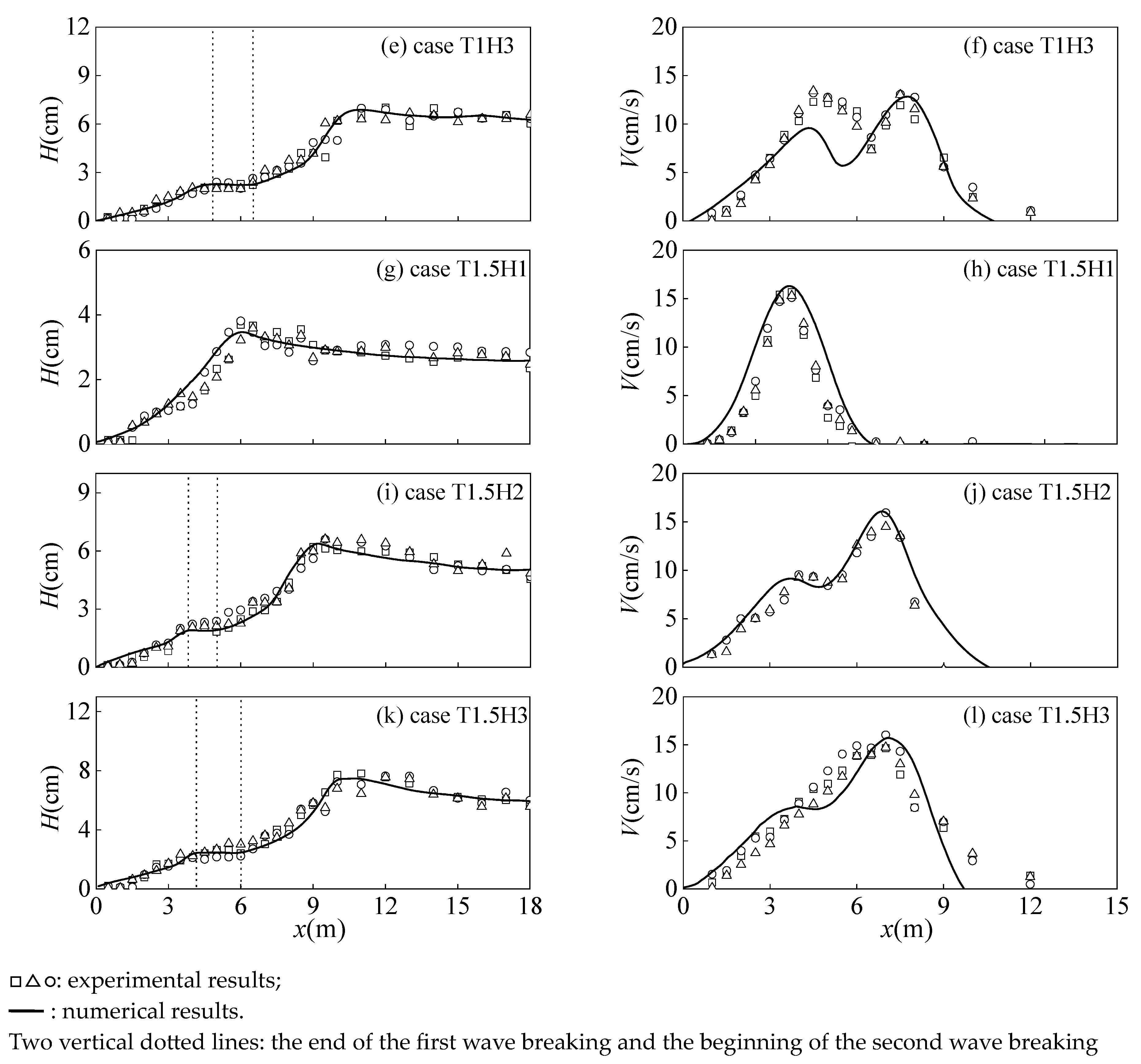
4.2. Validation for Different Incident Wave Heights

In order to verify the applicability of this model to different incident wave heights, this section simulates the experimental results of different incident wave heights for experimental cases with periods of 1 s and 1.5 s. The model is validated by comparing the simulation results with the experimental results.

Figure 10 shows the comparison of the numerical results and experimental results for different incident wave heights. It can be seen from Figure 10a,g that the wave conditions with smaller incident wave heights only occur in the case of one wave breaking, and there is no wave recovery. This is because the ratio of wave height to water depth after wave breaking is an unsatisfactory judgment condition for wave recovery, as shown in Equation (21); therefore, there is no wave recovery for small wave heights. The longshore currents shown in Figure 10b,h have unimodal distributions, with the numerical simulation results being broader than the experimental results. For the cases with larger wave heights, it can be seen from the figure that the wave heights all show wave recovery, with a bimodal distribution being observed in the case of longshore currents. Comparing Figure 10c,e and Figure 10i,k, it can be seen that for the same wave period, the larger the wave height, the earlier the wave breaks, and the earlier the second breaking, the distance between the first and second breaking increases with increasing wave height. The distance to wave recovery increases with the increase in wave height, indicating that the distance to wave recovery is proportional to wave height. The calculated results are consistent with the experimental results. The distribution of longshore currents is slightly different from the experimental results. It can be seen from Figure 10d that at x = 8–9 m, the numerical results are broader than the experimental results in terms of longshore current distribution. Figure 10f shows that the secondary peak of the numerical results is smaller than the experimental results, while the main peak is consistent with the experimental results. Figure 10j shows that the numerical results are broader than the experimental results in terms of the longshore current distribution. Figure 10l shows that there is no obvious bimodal distribution in the experimental results, but there is a clear bimodal distribution in the numerical results. This is because one set of experimental results showed a trend towards a bimodal distribution but was covered by another set of results; therefore, there was no obvious bimodal distribution evident in the figure. The numerical results are narrower than the experimental results at x = 9–12 m; however, the overall trend is consistent.

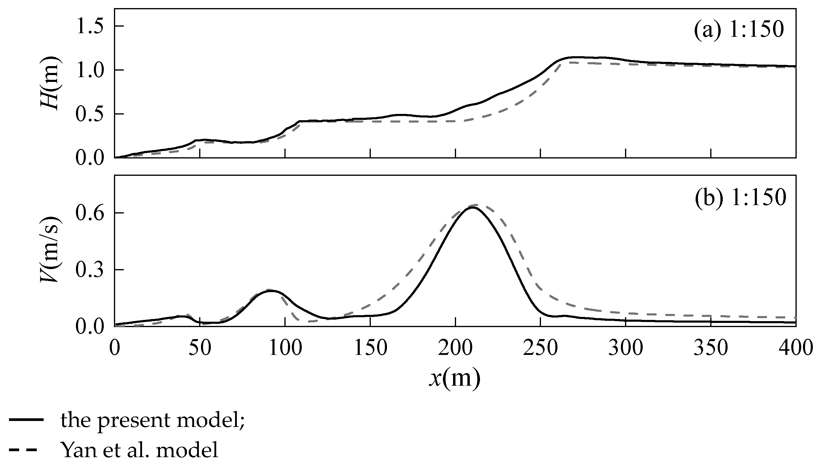
4.3. Comparison of Different Slopes

To verify the applicability of this model to different slopes, this section contains the numerical simulations relating to a planar slope beach topography with different slopes and presents a comparison of the computational results of this model with the results obtained by Yan et al. [10] using a wave averaging model. The wave conditions considered here are regular waves with a depth of 5 m, a period of 5 s, an incident wave height of 1.0 m, and slopes of 1:150, 1:300, and 1:500, respectively. The spatial steps are $\Delta x=0.6 \mathrm{m}$ and $\Delta y=1.2 \mathrm{m}$, and the time step is $\Delta t=0.05 \mathrm{s}$.

Figure 11 shows the distribution of the wave height and longshore current. It can be seen from Figure 11a that the location of wave recovery in this model is different from that of Yan et al. [10]. The location of wave recovery in Yan et al. [10] is about x = 200 m, while the location of wave recovery in this model is about x = 140 m. This may be due to the relatively low setting of the wave breaking intensity coefficient, which makes the breaking intensity insufficient during model calculation. In Figure 11b, the width of the distribution of the longshore current in this model is smaller than that of Yan et al. [10], but the location of the peak of the longshore current is consistent.

To address the issue of insufficient wave breaking intensity shown in Figure 11a, we discuss two parameters: the bottom friction coefficient $f_w$ and the wave breaking intensity coefficient $\sigma$. First, when $\sigma =1.0$, $f_w$ is set to 0.003, 0.006, and 0.009, respectively. Figure 12 shows the distributions of wave height and longshore current velocity for different bottom friction coefficients. It can be seen from the figure that the bottom friction coefficient has a small impact on wave height, and the longshore current velocity is inversely proportional to the bottom friction coefficient. When $f_w=0.006$, $\sigma$ is set to 1.0, 1.3, and 1.6, respectively. Figure 13 shows the distribution of wave height and longshore current velocity under different wave breaking intensity coefficients. It can be seen from the figure that as the breaking intensity coefficient increases, the attenuation after wave breaking also increases, and this also causes the longshore current velocity to increase. Therefore, by increasing the bottom friction and breaking strength coefficients, the calculation results of this model are closer to the results obtained by Yan et al. [10]. The above comparison with the calculation results of the model by Yan et al. [10] proves that this model is also applicable to the calculation of multiple wave breakings on different slopes. After comparison, here choose $\sigma =1.6$ and $f_w=0.01$. The case of gently sloping terrain with gradients of 1:300 and 1:500 is simulated below.

Figure 14 shows the calculation results of this model and the model used by Yan et al. [10] for different slopes. In Figure 11a, at x = 520 m and 230 m, this model simulates multiple wave breakings, but at x = 110 m and 55 m, there is no significant wave breaking phenomenon in this model, and the results obtained by Yan et al. [10] show significant wave breaking phenomena. This may be due to the different breaking methods used in the two models. Yan et al. [10] determined wave breaking based on the ratio of wave height to water depth and immediately stopped breaking once the conditions for wave breaking were established, resulting in significant changes at each breaking point. This model uses a comparison between ${\eta }_t^{*}$ and ${\eta }_t$ to determine wave breaking, and according to expression (20), it can be seen that wave breaking does not stop immediately but gradually opens. The values at x = 110 m and 55 m are relatively small, leading to no significant wave breaking. In Figure 11b, the longshore current at the first peak is consistent with the results obtained by Yan et al. [10], but the second and subsequent peaks are gradually smaller than those obtained by Yan et al. [10]. This may be due to insufficient wave breaking intensity. The results in Figure 11c,d are also consistent with Figure 11a,b, although the wave height and longshore current velocity are smaller than those obtained by Yan et al. [10]. However, it can also be seen in the figure that wave breaking appears multiple times and the velocity of the longshore current has a multi-peak distribution. This also proves that the model developed in this study can describe the phenomenon of multiple wave breakings.

5. Model Application

In the case of multiple wave breakings on planar slope topography, wave height and longshore current velocity appear to have new distributional characteristics. This section discusses the distribution characteristics of wave height and longshore current velocity under the conditions of different wave incidence angles and wave periods using this model.

5.1. The Influence of Wave Incident Angles

Shen et al. [6] conducted experiments using a wave incidence angle of 30° only, and in order to study the influence of different incidence angles on wave height and longshore current velocity distributions under multiple wave breakings, this section takes the experimental wave condition of T1.5H3 as an example and adds four different incident angles 10°, 20°, 40°, and 50° for explanation.

Figure 15 shows the distributions of wave height and longshore current at different wave incidence angles. It can be seen from Figure 15a that the distribution of wave height does not change with the change in wave incidence angle. Figure 15b shows that the longshore current velocity increases with the increase in incident angle. The increase rate of longshore current velocity after the first breaking is significantly higher than that after the second breaking, but the location of the double peaks is unchanged. This is because the coast under consideration here has a straight isobath, and the oblique incidence of waves satisfies Snell’s law [28], as follows:

$$\frac{\sin \alpha }{c}=\frac{\sin {\alpha }_0}{c_0},$$

(24)

where ${\alpha }_0$ and $c_0$ are the wave direction angle and wave velocity in deep water, respectively, in shallow water $c\approx \sqrt{gh}$.

It can be seen from Formula (24) that the wave direction angle at different locations is proportional to the wave direction angle in deep water, while the longshore current velocity at the double-peak location is proportional to the value of $\sin \alpha$. Therefore, the longshore current velocity at the double-peak location increases with increasing wave incident angle, but the increase coefficients at different locations are different: $\sin {\alpha }_i=\sqrt{h_i/h_0}\sin {\alpha }_0$. This causes different growth rates in terms of longshore current velocity at different locations. To quantitatively illustrate this point,

Table 4. Values of $\sin \alpha$ for different wave incidence angles.

Wave Incidence Angle (°)	Primary Peak Location	Secondary Peak Location
10	0.108	0.071
20	0.213	0.139
30	0.312	0.204
40	0.401	0.262
50	0.477	0.313

gives the values of different wave incident angles at the location of the two peaks of the coastal current. It can be seen from the table that the difference in $\sin \alpha$ at the location of the two peaks increases with the increase in wave incident angle. When the wave incidence angle is 10°, the difference in $\sin \alpha$ at the location of the two peaks is 0.037; when the wave incidence angle is 50°, the difference in $\sin \alpha$ at the location of the two peaks is 0.164. Therefore, when the wave incident angle increases, the increase in longshore current velocity at the secondary peak is less than that at the primary peak.

5.2. The Influence of Wave Period

In order to study the influence of wave period on wave height and longshore current velocity, this section discusses two sets of wave conditions with similar wave heights: T1H2 and T1.5H2. Due to the fact that the wave heights in the experimental results are not exactly the same, the experimental wave height of 5.95 cm is also given here for the analysis of the numerical simulation results with periods of 1.0 s, 1.3 s, 1.6 s, and 1.9 s to study the influence of different wave periods.

Figure 16 shows the distributions of different wave heights and longshore currents for different wave periods. It can be seen from Figure 16a,c that as the wave period gradually increases, the wave height at the first breaking point also increases, and the location of the breaking point tends toward the offshore location. The wave period does not affect wave recovery, so the breaking of the second wave remains unchanged. This is due to the decreased water depth, where shoaling occurs, and the larger the wave period, the larger the shoaling coefficient. Wave height also increases. The reason why the second wave breaking remains unchanged is that under the action of the judgment condition for the wave recovery Equation (21), the location of wave recovery remains unchanged, so the wave height remains unchanged. It can be seen from Figure 16b,d that the period has a small impact on the velocity of the longshore current.

6. Conclusions

A computational model for multiple wave breakings has been studied. In the Boussinesq model, the wave breaking method combines Equation (19) with the wave recovery judgment condition Equation (21), enabling the judging of multiple wave breaking phenomena. The model is validated by comparing the calculation results with the experimental results, and the ability of the model to simulate multiple wave breakings is demonstrated by comparing the calculation results with those of the average wave model. The research conclusions are as follows:

(1)

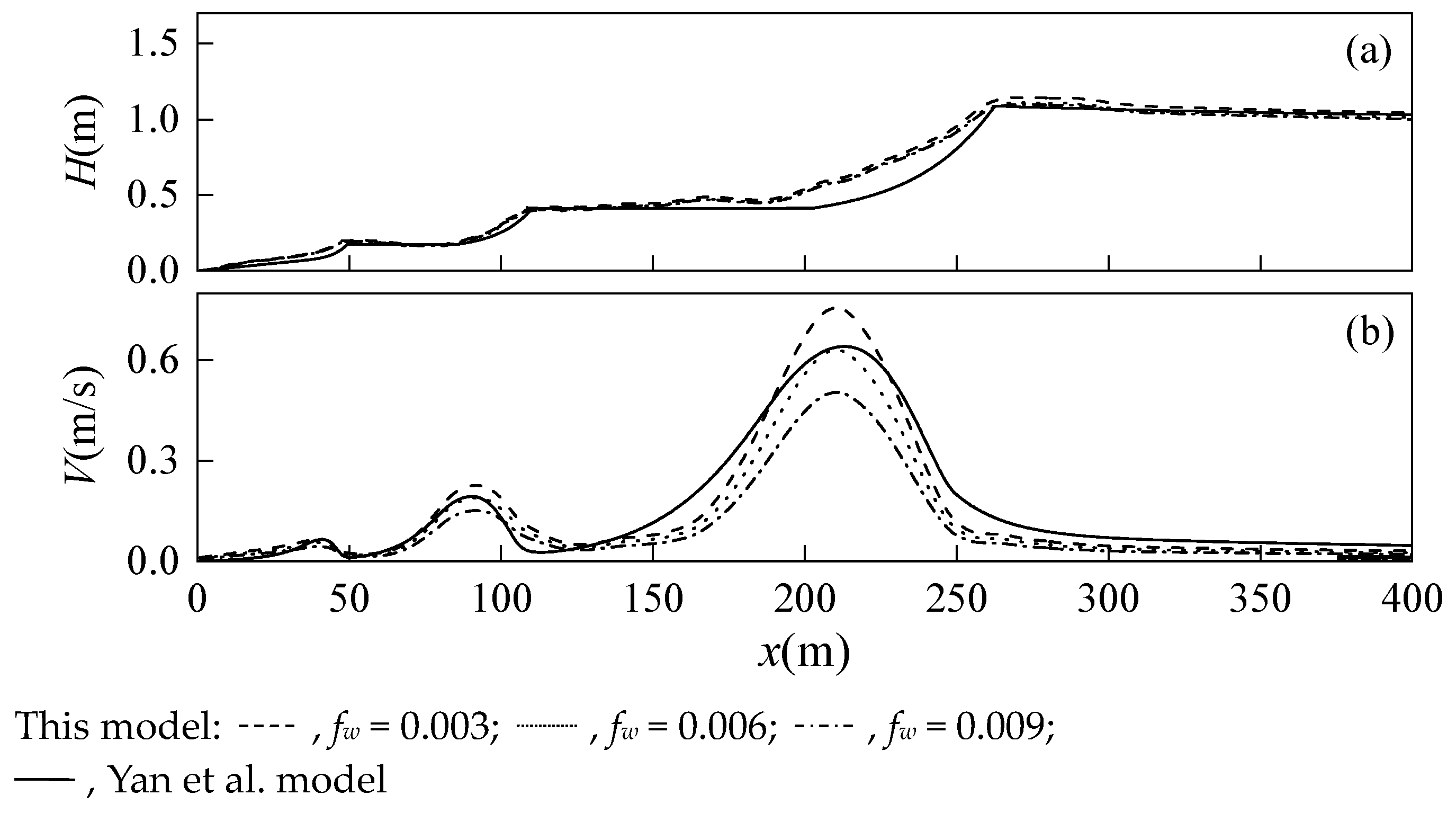
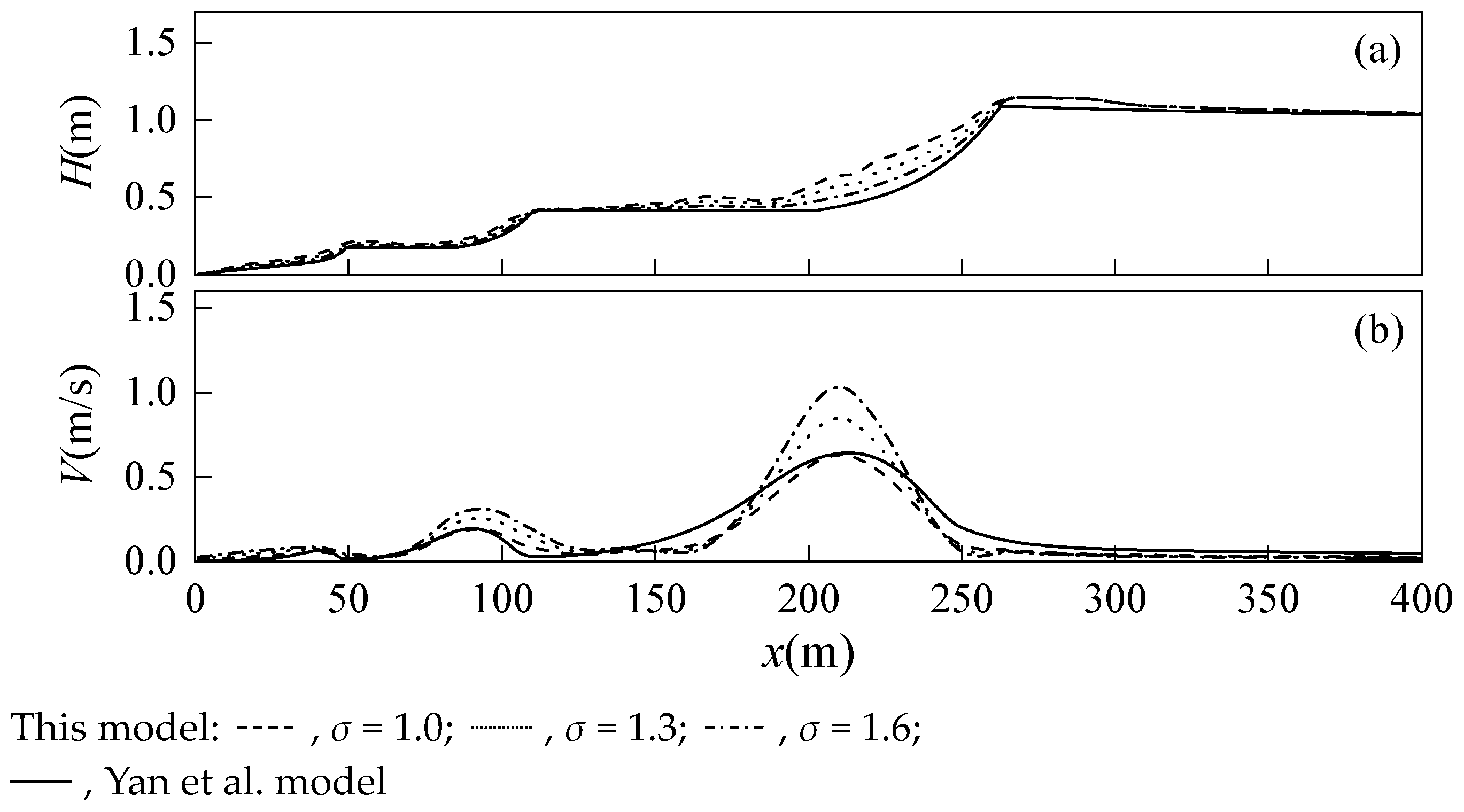
The wave recovery judgment condition Equation (21) applied to the wave average model is also applicable to the Boussinesq model. By modifying the wave breaking term during the wave breaking judgment process, the Boussinesq model has the ability to automatically judge wave recovery. This ability extends its previous ability to consider multiple wave breakings in sandbar topography conditions to multiple wave breakings in general situations (planar slope topography). By modifying the wave breaking term Equation (22), wave height can reach a balanced state of neither increasing nor decreasing during the wave recovery stage, and the comparison with experimental results also proves that this modification is reasonable. The general wave breaking judgment method Equation (19) can be applied to new wave breaking that occurs after the end of wave recovery.

(2)

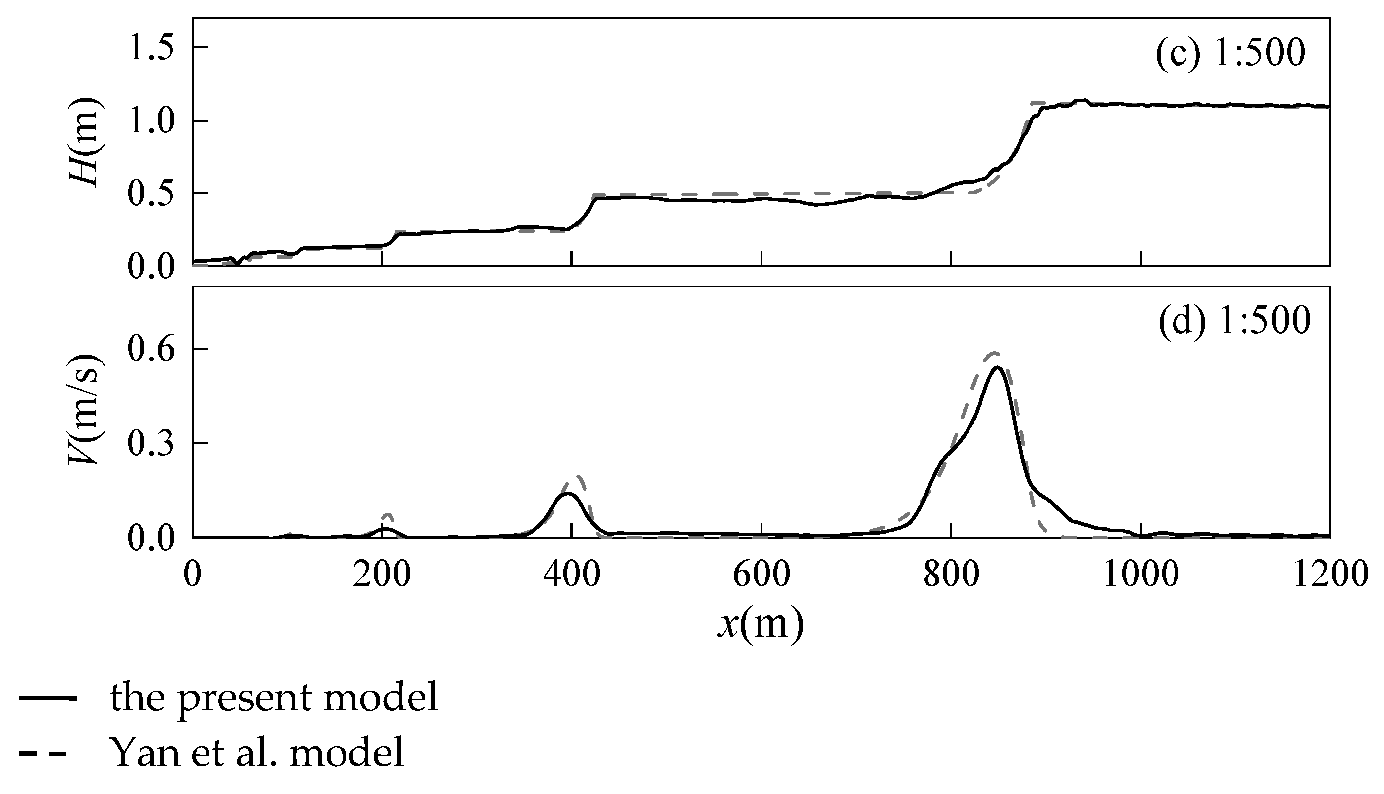
The verification of different wave heights and slopes shows that this model can not only simulate the gentle topography with a slope of 1:100 in the experiment but also has the ability to simulate multiple wave breaks for gentler slopes of 1:300 and 1:500.

(3)

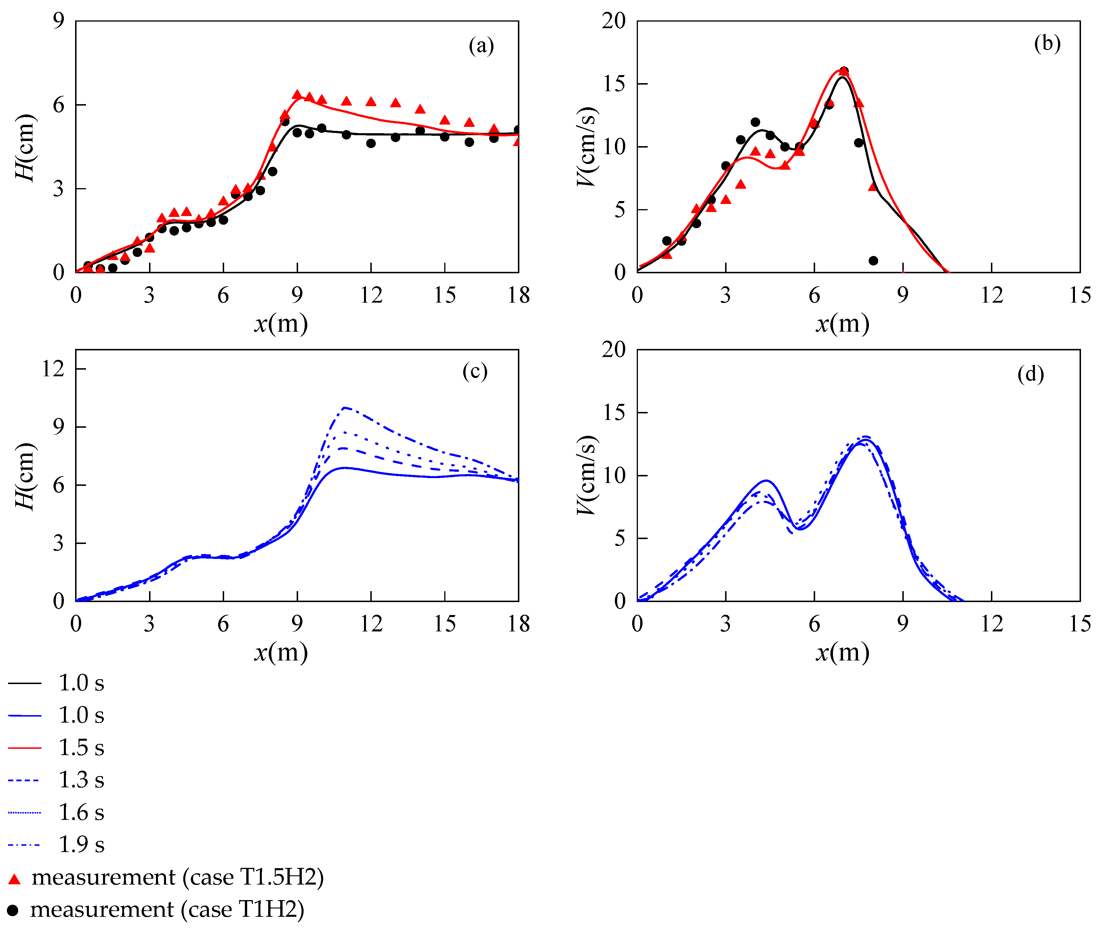
In the case of multiple wave breakings, the distribution of wave height does not change with the change in wave incident angle, while the distribution of longshore current velocity increases with the increase in wave incident angle; but the location of the double peak of the longshore current velocity remains unchanged, with the growth rate of the main peak being greater than that of the secondary peak, which makes the double-peak distribution of the longshore current velocity more obvious. The influence of wave period on the distribution of wave height is greater than that on the distribution of the longshore current velocity, which is manifested in the increase in wave height at the first breaking point with the increase in wave period and the trend toward offshore movement. The second breaking point is affected by wave recovery, and there is no obvious trend of change in terms of wave height. The distribution of the longshore current velocity is less affected by period and there is no significant change in the position of the double peak, with it only having some influence on the shape of the second peak.

The above provides the distribution of coastal current velocities of multiple wave breakings under different conditions. In practical applications, the distribution of coastal current velocities calculated by numerical methods can be used to predict the transport patterns of coastal materials, such as sediment movement and pollutant diffusion trajectories. In seawater, suspended matter refers to organic and inorganic particulate matter in water, which is one of the material components of seawater and an important carrier for many microorganisms, affecting the marine ecological environment and the exchange of substances between inland and ocean. At the same time, the transport process of suspended matter can reflect the characteristics of ocean hydrodynamics, affecting the shaping of submarine topography and the changes in coastlines. Coastal currents are the main driving forces affecting the distribution and transport processes of suspended matter in coastal waters. Therefore, the characteristics of the distribution of coastal current velocities of multiple wave breakings play an important role in studying the evolution of coastal landforms.

References

1. Li, Y.; Yu, Y.; Cui, L.; Dong, G. Experimental study of wave breaking on gentle slope. China Ocean Eng. 2000, 14, 59–67. [Google Scholar]
2. Church, J.C.; Thornton, E.B. Effects of breaking wave induced turbulence within a longshore current model. Coast. Eng. 1993, 20, 1–28. [Google Scholar] [CrossRef]
3. Rogers, A.L.; Ravens, T.M. Measurement of Longshore Sediment Transport Rates in the Surf Zone on Galveston Island, Texas. J. Coast. Res. 2008, 24, 62–73. [Google Scholar] [CrossRef]
4. Reniers, A.J.H.M.; Battjes, J.A. A laboratory study of longshore currents over barred and non-barred beaches. Coast. Eng. 1997, 31, 1–21. [Google Scholar] [CrossRef]
5. Baum, S.K.; Basco, D.R. A Numerical Investigation of the Longshore Current Profile for Multiple Bar/Trough Beaches. In Proceedings of the 20th International Conference on Coastal Engineering, Taipei, Taiwan, 9–14 November 1986; pp. 971–985. [Google Scholar]
6. Karjadi, E.A.; Kobayashi, N. Time-Dependent Quasi-3D Modeling of Breaking Waves on Beaches. In Coastal Engineering; ASCE: Reston, VA, USA, 2015; pp. 233–246. [Google Scholar] [CrossRef]
7. Chen, Q.; Kirby, J.T.; Dalrymple, R.A.; Kennedy, A.B.; Thornton, E.B.; Shi, F. Boussinesq modelling of waves and longshore currents under field conditions. In Proceedings of the 27th Conference on Coastal Engineering, Sydney, Australia, 16–21 July 2000. [Google Scholar] [CrossRef]
8. Elsayed, S.M.; Gijsman, R.; Schlurmann, T.; Goseberg, N. Nonhydrostatic Numerical Modeling of Fixed and Mobile Barred Beaches: Limitations of Depth-Averaged Wave Resolving Models around Sandbars. J. Waterw. Port Coast. Ocean Eng. 2022, 148, 04021045. [Google Scholar] [CrossRef]
9. Shen, L.D.; Gui, Q.; Zou, Z.L.; He, L.L.; Chen, W.; Jiang, M. Experimental study and numerical simulation of mean longshore current for mild slope. Wave Motion 2020, 99, 102651. [Google Scholar] [CrossRef]
10. Yan, S.; Zou, Z.L.; Shen, L.D.; Wang, Y. A Calculation Model for Multiple-Breaking Waves and Wave-induced Currents on Very Gentle Beaches. J. Waterw. Port Coast. Ocean Eng. 2021, 147, 04021017. [Google Scholar] [CrossRef]
11. Tajima, Y.; Madsen, O.S. Modeling near-shore waves, surface rollers, and undertow velocity profiles. J. Waterw. Port Coast. Ocean Eng. 2006, 132, 429–438. [Google Scholar] [CrossRef]
12. Dutykh, D.; Katsaounis, T.; Mitsotakis, D. Finite volume schemes for dispersive wave propagation and runup. J. Comput. Phys. 2011, 230, 3035–3061. [Google Scholar] [CrossRef]
13. Abroug, I.; Abcha, N.; Dutykh, D.; Jarno, A.; Marin, F. Experimental and numerical study of the propagation of focused wave groups in the nearshore zone. Phys. Lett. A 2020, 384, 126144. [Google Scholar] [CrossRef]
14. Abdalazeez, A.; Didenkulova, I.; Dutykh, D. Dispersive Effects During Long Wave Run-up on a Plane Beach. In Advances in Natural Hazards and Hydrological Risks: Meeting the Challenge; Fernandes, F., Malheiro, A., Chaminé, H., Eds.; Springer: Cham, Switzerland, 2020; pp. 143–146. [Google Scholar] [CrossRef]
15. Clamond, D.; Dutykh, D.; Mitsotakis, D. A Variational Approach to Water Wave Modelling (Vol. 3); International Association for Hydro-Environment Engineering and Research (IAHR): Madrid, Spain, 2024. [Google Scholar] [CrossRef]
16. van Groesen, E.; Andonowati, A. Hamiltonian Boussinesq formulation of wave–ship interactions. Appl. Math. Model. 2016, 42, 133–144. [Google Scholar] [CrossRef]
17. Tuozzo, S.; Di Leo, A.; Buccino, M.; Calabrese, M. Boussinesq Modelling of Shallow Water Phenomena. Environ. Sci. Proc. 2022, 21, 64. [Google Scholar] [CrossRef]
18. Postacchini, M.; Melito, L.; Ludeno, G. Nearshore Observations and Modeling: Synergy for Coastal Flooding Prediction. J. Mar. Sci. Eng. 2023, 11, 1504. [Google Scholar] [CrossRef]
19. Mesloub, S.; Gadain, H.E. On Some Initial and Initial Boundary Value Problems for Linear and Nonlinear Boussinesq Models. Symmetry 2019, 11, 1273. [Google Scholar] [CrossRef]
20. Wingate, B.A.; Rosemeier, J.; Haut, T. Mean Flow from Phase Averages in the 2D Boussinesq Equations. Atmosphere 2023, 14, 1523. [Google Scholar] [CrossRef]
21. Dalrymple, R.A.; Liu, L.F. Waves over Soft Muds: A Two-Layer Fluid Model. J. Phys. Oceanogr. 1978, 8, 1121–1131. [Google Scholar]
22. Zou, Z.L.; Fang, K.Z. Alternative forms of the higher-order Boussinesq equations: Derivations and validations. Coast. Eng. 2008, 55, 506–521. [Google Scholar] [CrossRef]
23. Kennedy, A.B.; Chen, Q.; Kirby, J.T.; Dalrymple, R.A. Boussinesq modeling of wave transformation, breaking and runup. I: One dimension. J. Waterw. Port Coast. Ocean Eng. 2000, 126, 39–47. [Google Scholar] [CrossRef]
24. Gobbi, M.F.; Kirby, J.T. Wave evolution over submerged sills: Tests of a high-order Boussinesq model. Coast. Eng. 1999, 37, 57–96. [Google Scholar] [CrossRef]
25. Kim, G.; Lee, C.; Suh, K.D. Generation of random waves in time-dependent extended mild-slope equations using a source function method. Ocean Eng. 2006, 33, 2047–2066. [Google Scholar] [CrossRef]
26. Chen, Q.; Kirby, J.T.; Dalrymple, R.A.; Kennedy, A.B.; Chawla, A. Boussinesq modeling of wave transformation, breaking and runup. II: Two horizontal dimensions. J. Waterw. Port Coast. Ocean Eng. 2000, 126, 48–56. [Google Scholar] [CrossRef]
27. Willmott, C.J. On the validation of models. Phys. Geogr. 1981, 2, 184–194. [Google Scholar] [CrossRef]
28. Li, X.; Zhang, W. Application of Snell’s law in reflection raytracing using the multistage fast marching method. Earthq. Res. Adv. 2021, 1, 100009. [Google Scholar] [CrossRef]
Figure 1. Plan view of the experimental layout for the planar beach.
Jmse 12 00860 g001
Figure 2. Distribution of wave height for different wave conditions (ai).
Jmse 12 00860 g002aJmse 12 00860 g002b
Figure 3. Distribution of longshore current for different wave conditions (ai).
Jmse 12 00860 g003
Figure 4. Distribution of wave height on the sand bar and planar slope topography.
Jmse 12 00860 g004
Figure 5. Time series of η t * and η t at different locations: (ae) sand bar; (fj) planar slope.
Jmse 12 00860 g005
Figure 6. The computation domain.
Jmse 12 00860 g006
Figure 7. Distribution of wave height and time-averaged flow field: (a) periodic boundary and (b) solid boundary.
Jmse 12 00860 g007
Figure 8. Comparison between numerical and experimental results of wave height (a) and longshore current (b).
Jmse 12 00860 g008
Figure 9. Arrangement of wave gauges (above) and the time series of free surface elevation at different locations (below).
Jmse 12 00860 g009aJmse 12 00860 g009b
Figure 10. Comparison of numerical results and experimental results for different incident wave heights (a,c,e,g,i,k) and (b,d,f,h,j,l) longshore currents.
Jmse 12 00860 g010aJmse 12 00860 g010b
Figure 11. Distribution of wave height (a) and longshore current (b) for slope 1:150; Yan et al.: [10].
Jmse 12 00860 g011
Figure 12. Distribution of wave height (a) and longshore current (b) for different bottom friction coefficients; Yan et al.: [10].
Jmse 12 00860 g012
Figure 13. Distribution of wave height (a) and longshore current (b) for different breaking intensity coefficients; Yan et al.: [10].
Jmse 12 00860 g013
Figure 14. Comparison of calculation results of different models for different slopes: (a,b) 1:300 slope and (c,d) 1:500; Yan et al.: [10].
Jmse 12 00860 g014aJmse 12 00860 g014b
Figure 15. Distributions of wave height (a) and longshore current (b) for different wave incidence angles.
Jmse 12 00860 g015
Figure 16. Distributions of wave height and longshore current for different wave periods: (a) wave heights distribution of experimental wave conditions; (b) longshore currents distribution of experimental wave conditions; (c) wave heights distribution of numerical simulation; (d) Numerical simulation of longshore currents distribution.
Jmse 12 00860 g016