Numerical Investigation of the Seabed Dynamic Response to a Perforated Semi-Circular Breakwater

Abstract

The semi-circular breakwater (SBW) has been implemented at numerous global locations due to its outstanding wave dissipation effectiveness and high structural performance. This study extends prior research by investigating the seabed dynamic response and hydrodynamic response characteristics around perforated SBWs. A coupled numerical model is developed to integrate waves, a semi-circular breakwater, and a sandy seabed. Wave behavior is simulated using Reynolds-averaged Navier–Stokes equations with a k-ε turbulence closure scheme, and the seabed response is numerically simulated using Biot’s full-dynamic (u-w) equations. After verifying computational accuracy, a series of tests is conducted to explore the effects of marine environments and SBW characteristics. Test results reveal a positive correlation between seabed response and wave height, wave period, and perforation number, while showing a negative correlation between seabed response and water depth and perforation rate. The basic perforation type is more effective than front and rear perforation types in maintaining a stable flow field and seabed response. These findings provide insights for designing SBWs for effective wave dissipation and seabed stability in complex marine environments, offering valuable recommendations for future designs.

1. Introduction

The semi-circular breakwater is a new structure that was initially developed and has been extensively studied in Japan in recent years [1]. This structure demonstrates excellent effectiveness in wave dissipation, stability, and cost-effectiveness. It is suitable for deployment in environments characterized by significant waves and unstable seabed foundations [2,3]. SBWs are classified into impermeable, front perforation (seaside wall perforated), rear perforation (leeside wall perforated), and basic perforation types (both seaside and leeside walls perforated) [4]. In actual marine environments, waves and current flows coexist. The combined loading induces significant fluctuations in pore water pressure and effective stresses within the seabed [5,6,7]. Therefore, it is crucial to investigate the seabed response characteristics around SBWs under wave–current interaction.

To enhance the understanding of the seabed response to wave action, extensive experiments and numerical studies have been conducted over the past decades. Mynett et al. [8] investigated the pore water pressure and stress distribution in a saturated seabed beneath vertical caissons using boundary layer theory. Tsai et al. [9] expanded this model to an infinite-thickness scenario and modified the breakwater from a caisson type to a composite type. Mase et al. [10] investigated the pore water pressure and effective stress distribution around perforated breakwaters using Biot’s consolidation theory. They revealed the significant influence of the breakwater’s perforation rate on pore water pressure and phase lag phenomena. Jeng et al. [11,12] proposed the GFEM–WSSI finite element model to simulate the pore water pressure distribution in the seabed beneath composite breakwaters. They conducted a comparative analysis of pore water pressure distribution and explored the impact of wave and seabed parameters on the seabed response. Zhang et al. [13] conducted numerical simulations to study the seabed response to perforated breakwaters, specifically discussing the influence of wave period and wave height on seabed pore water pressure. Zhang et al. [14] and Zhao et al. [15] extended a two-dimensional wave–structure–seabed model to a three-dimensional model. They numerically simulated the seabed dynamic response and investigated the effects of wave and seabed characteristics. Building upon the model proposed by Mizutani et al. [16], Mostafa et al. [17] developed a coupled (BEM–FEM) model to study wave–breakwater–seabed interaction. They conducted experimental studies on the deformation of caisson breakwaters and analyzed pore pressure distribution. Yan et al. [18] conducted model experiments to investigate the stability of a silty clay seabed around SBWs. They focused on the pore pressure around breakwaters and the seabed shear failure induced by the destruction of the soil fabric.

In addition, wave reflection can significantly impact the seabed dynamic response, potentially leading to severe coastal erosion [19]. Xu et al. [20] conducted flume experiments to investigate the Bragg resonance reflection of wave propagation over submerged breakwaters. They discussed the influence of the permeability, relative width, relative height, and cross-sectional shapes of submerged breakwaters on Bragg resonance reflection. Brunone et al. [21] developed a rational definition of the relevant characteristics of wave–structure interaction. They proposed a second-order model to describe the flow field characteristics on a steep slope.

This study uses a coupled numerical model to investigate the dynamic response of a sandy seabed. Reynolds-averaged Navier–Stokes equations (RANS) are used to model wave–current behavior. Meanwhile, 3D full-dynamic (u-w) governing equations based on Biot’s poro-elastic theory are adopted for modeling the seabed response. Due to the inadequacy of the existing research on the seabed response surrounding SBWs, this study investigates the influence of marine environments and SBW characteristics on the seabed dynamic response.

The rest of this paper is organized as follows: Section 2 introduces both the flow model and the seabed model. Model validation and numerical setup are presented in Section 3. Section 4 discusses the effects of the coupled wave–seabed–structure model under different wave conditions and breakwater structures. Section 5 provides the conclusion and offers recommendations.

2. Numerical Model

2.1. Flow Model

Numerical simulations are based on Reynolds-averaged Navier–Stokes equations (RANS), which describe the movement of a wave-induced fluid.

In this study, solid geometry is represented using area and volume fractions on Cartesian meshes to enhance calculation efficiency and accuracy. The model equations are as follows:

$$\frac{\partial }{\partial \mathrm{x}}\left({\mathrm{v}}_{\mathrm{x}}{\mathrm{A}}_{\mathrm{x}}\right)+\frac{\partial }{\partial \mathrm{y}}\left({\mathrm{v}}_{\mathrm{y}}{\mathrm{A}}_{\mathrm{y}}\right)+\frac{\partial }{\partial \mathrm{z}}\left({\mathrm{v}}_{\mathrm{z}}{\mathrm{A}}_{\mathrm{z}}\right)=0$$

(1)

$$\frac{\partial {\mathrm{v}}_{\mathrm{x}}}{\partial \mathrm{t}}+\frac{1}{{\mathrm{V}}_{\mathrm{F}}}\left\{{\mathrm{v}}_{\mathrm{x}}{\mathrm{A}}_{\mathrm{x}}\frac{\partial {\mathrm{v}}_{\mathrm{x}}}{\partial \mathrm{x}}+{\mathrm{v}}_{\mathrm{y}}{\mathrm{A}}_{\mathrm{y}}\frac{\partial {\mathrm{v}}_{\mathrm{x}}}{\partial \mathrm{y}}+{\mathrm{v}}_{\mathrm{z}}{\mathrm{A}}_{\mathrm{z}}\frac{\partial {\mathrm{v}}_{\mathrm{x}}}{\partial \mathrm{z}}\right\}=-\frac{1}{{\mathsf{\rho }}_{\mathrm{f}}}\frac{\partial \mathrm{p}}{\partial \mathrm{x}}+{\mathrm{f}}_{\mathrm{x}}$$

(2)

$$\frac{\partial {\mathrm{v}}_{\mathrm{y}}}{\partial \mathsf{\iota }}+\frac{1}{{\mathrm{V}}_{\mathrm{F}}}\left\{{\mathrm{v}}_{\mathrm{x}}{\mathrm{A}}_{\mathrm{x}}\frac{\partial {\mathrm{v}}_{\mathrm{y}}}{\partial \mathrm{x}}+{\mathrm{v}}_{\mathrm{y}}{\mathrm{A}}_{\mathrm{y}}\frac{\partial {\mathrm{v}}_{\mathrm{y}}}{\partial \mathrm{y}}+{\mathrm{v}}_{\mathrm{z}}{\mathrm{A}}_{\mathrm{z}}\frac{\partial {\mathrm{v}}_{\mathrm{y}}}{\partial \mathrm{z}}\right\}=-\frac{1}{{\mathsf{\rho }}_{\mathrm{f}}}\frac{\partial \mathrm{p}}{\partial \mathrm{y}}+{\mathrm{f}}_{\mathrm{y}}$$

(3)

$$\frac{\partial {\mathrm{v}}_{\mathrm{z}}}{\partial \mathrm{t}}+\frac{1}{{\mathrm{V}}_{\mathrm{F}}}\left\{{\mathrm{v}}_{\mathrm{x}}{\mathrm{A}}_{\mathrm{x}}\frac{\partial {\mathrm{v}}_{\mathrm{z}}}{\partial \mathrm{x}}+{\mathrm{v}}_{\mathrm{y}}{\mathrm{A}}_{\mathrm{y}}\frac{\partial {\mathrm{v}}_{\mathrm{z}}}{\partial \mathrm{y}}+{\mathrm{v}}_{\mathrm{z}}{\mathrm{A}}_{\mathrm{z}}\frac{\partial {\mathrm{v}}_{\mathrm{z}}}{\partial \mathrm{z}}\right\}=-\frac{1}{{\mathsf{\rho }}_{\mathrm{f}}}\frac{\partial \mathrm{p}}{\partial \mathrm{z}}+\mathrm{g}+{\mathrm{f}}_{\mathrm{z}}$$

(4)

where x, y, and z are longitudinal, vertical, and spanwise directions, respectively; v_x, v_y, and v_z are longitudinal, vertical, and spanwise velocities, respectively; ${\mathrm{V}}_{\mathrm{F}}$ is the flowable volume fraction in FAVOR grid processing; A_x, A_y, and A_z are the fractions of flowable area in x, y, and z directions, respectively, in grid processing; ${\mathsf{\rho }}_{\mathrm{f}}$ is the density of the fluid; p is the pressure; g is the gravitational acceleration; and ${\mathrm{f}}_{\mathrm{x}}$, ${\mathrm{f}}_{\mathrm{y}}$, and ${\mathrm{f}}_{\mathrm{z}}$ are the acceleration of viscous forces in the x, y, and z directions, respectively.

The RNG k–ε turbulence scheme proposed by Yakhot et al. [22,23] is used in this study. The model is derived from the transient Navier–Stokes equation using a mathematical method known as the renormalization group (RNG). The RNG k–ε model significantly enhances the simulation accuracy of fluid mechanics by incorporating the effects of large-scale movements and adjusting viscosity to account for small-scale effects. It systematically eliminates small-scale movements from the control equation, thereby improving the simulation performance for transient flow and flow with bending characteristics. The prognostic equations of turbulent kinetic energy and its dissipation rate can be written as:

$$\frac{\partial {\mathrm{k}}_{\mathrm{T}}}{\partial \mathrm{t}}+\frac{1}{{\mathrm{V}}_{\mathrm{F}}}\left({\mathrm{v}}_{\mathrm{x}}{\mathrm{A}}_{\mathrm{x}}\frac{\partial {\mathrm{k}}_{\mathrm{T}}}{\partial \mathrm{x}}+{\mathrm{v}}_{\mathrm{y}}{\mathrm{A}}_{\mathrm{y}}\frac{\partial {\mathrm{k}}_{\mathrm{T}}}{\partial \mathrm{y}}+{\mathrm{v}}_{\mathrm{z}}{\mathrm{A}}_{\mathrm{z}}\frac{\partial {\mathrm{k}}_{\mathrm{T}}}{\partial \mathrm{z}}\right)={\mathrm{P}}_{\mathrm{T}}+{\mathrm{G}}_{\mathrm{T}}+{\mathrm{D}}_{{\mathrm{k}}_{\mathrm{T}}}-{\mathsf{\epsilon }}_{\mathrm{T}}$$

(5)

$$\frac{\partial {\mathsf{\epsilon }}_{\mathrm{T}}}{\partial \mathrm{t}}+\frac{1}{{\mathrm{V}}_{\mathrm{F}}}\left({\mathrm{v}}_{\mathrm{x}}{\mathrm{A}}_{\mathrm{x}}\frac{\partial {\mathsf{\epsilon }}_{\mathrm{T}}}{\partial \mathrm{x}}+{\mathrm{v}}_{\mathrm{y}}{\mathrm{A}}_{\mathrm{y}}\frac{\partial {\mathsf{\epsilon }}_{\mathrm{T}}}{\partial \mathrm{y}}+{\mathrm{v}}_{\mathrm{z}}{\mathrm{A}}_{\mathrm{z}}\frac{\partial {\mathsf{\epsilon }}_{\mathrm{T}}}{\partial \mathrm{z}}\right)=\frac{{\mathrm{C}}_1\cdot {\mathsf{\epsilon }}_{\mathrm{T}}}{{\mathrm{k}}_{\mathrm{T}}}\left({\mathrm{P}}_{\mathrm{T}}+{\mathrm{C}}_3\cdot {\mathrm{G}}_{\mathrm{T}}\right)+{\mathrm{D}}_{\mathsf{\epsilon }}-{\mathrm{C}}_2\frac{{\mathsf{\epsilon }}_{\mathrm{T}}}{{\mathrm{k}}_{\mathrm{T}}}$$

(6)

where ${\mathrm{C}}_1$, ${\mathrm{C}}_2$, and ${\mathrm{C}}_3$ are empirical constants; ${\mathrm{k}}_{\mathrm{T}}$ is the turbulent kinetic energy; ${\mathsf{\epsilon }}_{\mathrm{T}}$ is the turbulence dissipation; ${\mathrm{P}}_{\mathrm{T}}$ is the velocity-gradient-induced turbulence kinetic energy generation term; ${\mathrm{G}}_{\mathrm{T}}$ is the buoyancy production term; and ${\mathrm{D}}_{{\mathrm{k}}_{\mathrm{T}}}$ and ${\mathrm{D}}_{\mathsf{\epsilon }}$ are the diffusive terms.

This study uses the Euler method for free-surface tracking, incorporating the marker and cell (MAC) and the volume-of-fluid (VOF) methods. Fluid configurations are defined in terms of a VOF function F (x, y, z, t) [24], which represents the volume of fluid occupying a portion of unitary volume space. The fluid fraction F is a variable that depends on position coordinates and time, representing the ratio of fluid volume within the calculation unit to the total volume of the unit. The F value is 1 when the unit is full of fluid, 0 when there is no fluid in the unit, and between 0 and 1 when the unit contains free surfaces or bubbles. The fluid component F satisfies the transport equation:

$$\frac{\partial \mathrm{F}}{\partial \mathrm{t}}+\frac{1}{{\mathrm{V}}_{\mathrm{F}}}\left[\frac{\partial }{\partial \mathrm{x}}\left(\mathrm{F}{\mathrm{A}}_{\mathrm{x}}{\mathrm{v}}_{\mathrm{x}}\right)+\frac{\partial }{\partial \mathrm{y}}\left(\mathrm{F}{\mathrm{A}}_{\mathrm{y}}{\mathrm{v}}_{\mathrm{y}}\right)+\frac{\partial }{\partial \mathrm{z}}\left(\mathrm{F}{\mathrm{A}}_{\mathrm{z}}{\mathrm{v}}_{\mathrm{z}}\right)\right]=0$$

(7)

The position of the free surface is identified within units, where the F value ranges between 0 and 1. Since the fluid fraction F is a step function, numerical oscillations can easily occur at discontinuity points when using a differential scheme for a discrete solution, potentially compromising the original definition of the fluid fraction F. To mitigate this issue, Hirt and Nichols [24] proposed the VOF method and the donor–acceptor method for reconstructing the free surface.

2.2. Seabed Model

In numerical simulations, the seabed model is primarily solved using 3D full-dynamic (u-w) governing equations based on Biot’s poro-elastic theory [25,26]. Additionally, the model can be switched to the partly dynamic (u-p) mode or the quasi-static (Biot’s consolidation) mode as an optional configuration. The model is capable of simulating a wave-induced seabed response, wave–current interaction, and wave–structure interaction [27,28]. The model incorporates the inertia effects of both soil and pore fluid and accounts for the 3D fully non-homogeneous properties of the seabed and cross-anisotropic soil behavior. A notable advantage of the model is its capability to handle arbitrary wave–seabed–structure configurations through the material identification technique. The model can simulate a wave-induced seabed response with detailed physical resolutions, including pore pressure, effective stresses, displacements of soil and pore fluid, and seepage flow.

This study formulates three governing equations in tensor form for a problem involving wave–seabed–structure interaction, assuming the seabed is a porous elastic medium. These equations include the overall equilibrium equation of the soil, the equilibrium equation of pore fluid flow, and the mass balance equation:

$${\mathsf{\sigma }}_{\mathrm{ij},\mathrm{j}}+\mathsf{\rho }{\mathrm{g}}_{\mathrm{i}}=\mathsf{\rho }{\ddot{\mathrm{u}}}_{\mathrm{i}}+{\mathsf{\rho }}_{\mathrm{f}}{\ddot{\bar{\mathrm{w}}}}_{\mathrm{i}}$$

(8)

$$-{\mathrm{p}}_{,\mathrm{i}}+{\mathsf{\rho }}_{\mathrm{f}}{\mathrm{g}}_{\mathrm{i}}={\mathsf{\rho }}_{\mathrm{f}}{\ddot{\mathrm{u}}}_{\mathrm{i}}+\frac{{\mathsf{\rho }}_{\mathrm{f}}{\ddot{\bar{\mathrm{w}}}}_{\mathrm{i}}}{\mathrm{n}}+\frac{{\mathsf{\rho }}_{\mathrm{f}}{\mathrm{g}}_{\mathrm{i}}}{{\mathrm{k}}_{\mathrm{i}}}{\dot{\bar{\mathrm{w}}}}_{\mathrm{i}}$$

(9)

$$\stackrel{.}{{\dot{\mathsf{\epsilon }}}_{\mathrm{ii}}}+{\dot{\bar{\mathrm{w}}}}_{\mathrm{i},\mathrm{i}}=-\frac{\mathrm{n}}{{\mathrm{K}}_{\mathrm{f}}}\dot{\mathrm{p}}$$

(10)

where $\mathsf{\sigma }$ is the total stress, $\mathsf{\rho }$ is the total density of the porous medium, ${\mathsf{\rho }}_{\mathrm{f}}$ is the density of the fluid, g is the gravitational acceleration, ${\mathrm{u}}_{\mathrm{i}}$ is the displacement of the soil matrix, ${\mathrm{w}}_{\mathrm{i}}$ is the average relative displacement of the fluid to the solid skeleton, ${\mathrm{k}}_{\mathrm{i}}$ is the permeability of the porous medium, ${\mathrm{n}}_{\mathrm{e}}$ is the porosity of the solid phase, ${\mathrm{K}}_{\mathrm{f}}$ is the elastic modulus of the pore fluid, and $\epsilon$ is the strain of the soil skeleton.

In a natural non-homogeneous seabed, the permeability ($\mathrm{K}$) and Young’s modulus ($\mathrm{E}$) vary spatially. These parameters are spatially dependent on longitudinal, vertical, and spanwise coordinates in the model. This model considers the non-uniform distribution ($\mathrm{R}(\mathrm{x},\mathrm{y},\mathrm{z})$) of eight parameters: the density of the seabed (${\mathsf{\rho }}_{\mathrm{s}}$), the density of the fluid (${\mathsf{\rho }}_{\mathrm{f}}$), soil permeability ($\mathrm{K}$), the porosity of the solid phase ($\mathrm{n}$), the elastic modulus of the pore fluid (${\mathrm{K}}_{\mathrm{f}}$), Young’s modulus ($\mathrm{E}$), vertical Poisson’s ratio (${\mathrm{u}}_{\mathrm{hv}}$), and lateral Poisson’s ratio (${\mathrm{u}}_{\mathrm{hh}}$). The model is newly formulated to incorporate the spatial gradient of these non-uniform seabed parameters, resulting in the fully dynamic equations (Equations (11) and (12)):

$$\begin{array}{c}\mathrm{E}[{\displaystyle \sum _{\mathrm{s}=\mathrm{x},\mathrm{y},\mathrm{z}}}{\mathrm{C}}_{\mathrm{is}}\frac{{\partial }^2{\mathrm{u}}_{\mathrm{i}}}{\partial {\mathrm{s}}^2}+{\displaystyle \sum _{\mathrm{s}=\mathrm{y},\mathrm{z}}}\left({\mathrm{C}}_{\mathrm{is}}+{\mathrm{C}}_{\mathrm{ss}}\right)\frac{{\partial }^2{\mathrm{u}}_{\mathrm{s}}}{\partial \mathrm{i}\partial \mathrm{s}}+{\displaystyle \sum _{\mathrm{s}=\mathrm{x},\mathrm{y},\mathrm{z}}}\frac{\partial {\mathrm{C}}_{\mathrm{ss}}}{\partial \mathrm{i}}\frac{\partial {\mathrm{u}}_{\mathrm{s}}}{\partial \mathrm{s}}+{\displaystyle \sum _{\mathrm{s}=\mathrm{y},\mathrm{z}}}\frac{\partial {\mathrm{C}}_{\mathrm{is}}}{\partial \mathrm{s}}(\frac{\partial {\mathrm{u}}_{\mathrm{i}}}{\partial \mathrm{s}}+\frac{\partial {\mathrm{u}}_{\mathrm{s}}}{\partial \mathrm{i}}\left)\right]+\hfill \\ {\displaystyle \sum _{\mathrm{s}=\mathrm{y},\mathrm{z}}}{\mathrm{C}}_{\mathrm{is}}\frac{\partial \mathrm{E}}{\partial \mathrm{s}}(\frac{\partial {\mathrm{u}}_{\mathrm{s}}}{\partial \mathrm{n}}+\frac{\partial {\mathrm{u}}_{\mathrm{n}}}{\partial \mathrm{s}})+\frac{\partial \mathrm{E}}{\partial \mathrm{i}}{\displaystyle \sum _{\mathrm{s}=\mathrm{x},\mathrm{y},\mathrm{z}}}{\mathrm{C}}_{\mathrm{ss}}\frac{\partial {\mathrm{u}}_{\mathrm{s}}}{\partial \mathrm{s}}-\frac{\partial \mathrm{p}}{\partial \mathrm{x}}={\mathsf{\rho }}_{\mathrm{f}}\frac{{\partial }^2{\mathrm{w}}_{\mathrm{i}}}{\partial {\mathrm{t}}^2}+\mathsf{\rho }\frac{{\partial }^2{\mathrm{u}}_{\mathrm{i}}}{\partial {\mathrm{t}}^2}+{\mathrm{g}}_{\mathrm{i}}\hfill \end{array}$$

(11)

$$\begin{array}{c}{\mathrm{C}}_{\mathrm{xx}}={\mathrm{C}}_{\mathrm{yy}}=\frac{1-\mathsf{\mu }}{1-\mathsf{\mu }-{\mathsf{\mu }}^2}\hfill \\ {\mathrm{C}}_{\mathrm{zz}}=\frac{\mathsf{\mu }}{1-\mathsf{\mu }-{\mathsf{\mu }}^2}\hfill \\ {\mathrm{C}}_{\mathrm{xy}}={\mathrm{C}}_{\mathrm{yx}}=\frac{1}{2(1+\mathsf{\mu })}\hfill \\ {\mathrm{C}}_{\mathrm{xz}}={\mathrm{C}}_{\mathrm{yz}}={\mathrm{C}}_{\mathrm{zx}}={\mathrm{C}}_{\mathrm{zy}}=\frac{1}{2}(1+\mathsf{\mu })\hfill \end{array}$$

(12)

In this study, the flow model is used to analyze the hydrodynamic response characteristics around SBWs. The pressure data obtained from the analysis are integrated into the seabed model to determine the seabed response. Additionally, a comprehensive dynamic response model is used to evaluate the variation in liquefaction depth.

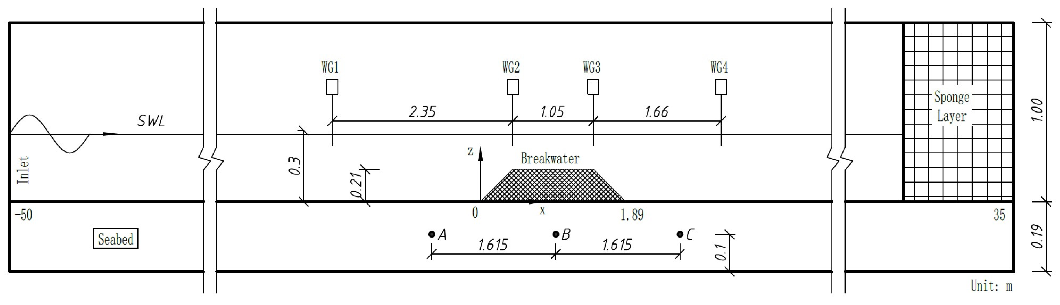
3. Model Validation and Numerical Setup

In this section, we use experimental studies by Mizutani et al. [29] and Wu and Hsiao [30] to validate numerical simulation results. These experiments specifically focus on permeable submerged breakwaters, making them valuable validations for the numerical model used in this study.

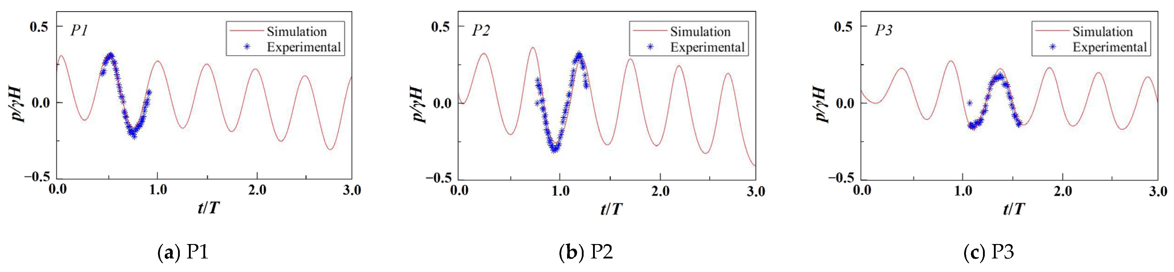
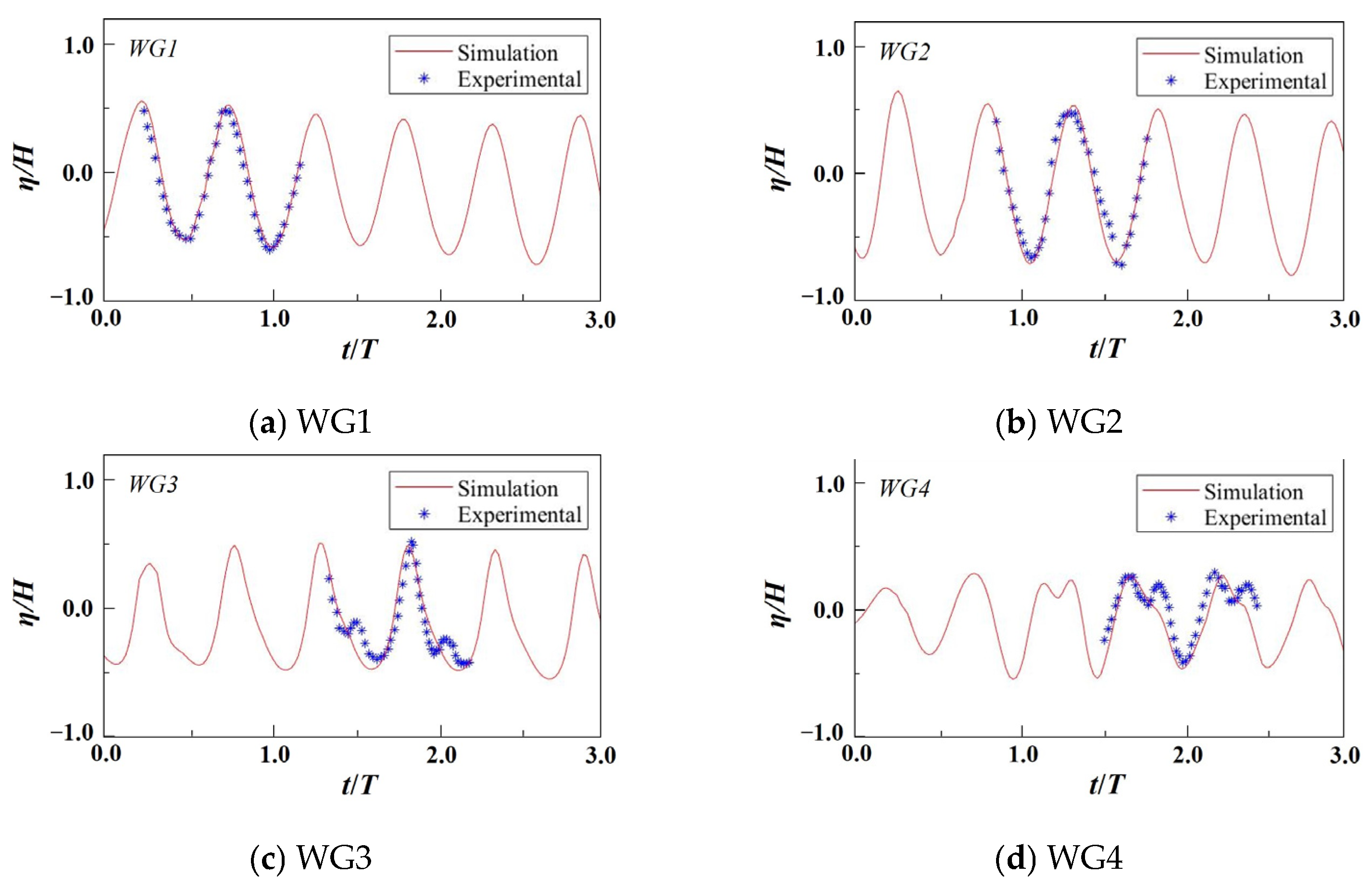
3.1. Model Validation

The experiments conducted by Mizutani et al. [29] investigated the interaction between regular waves, a sandy seabed, and a perforated SBW. Figure 1 shows a sketch of the numerical wave flume. Four gauges (WG1: x = −1.93 m; WG2: x = 0.42 m; WG3: x = 1.47 m; WG4: x = 3.13 m) are set up to measure the temporal evolution of the wave surface. The test conditions for the model validation are provided in

Table 1. Index properties of wave and breakwater structures.

Wave			Seabed Soil			Breakwater Soil
Wave Height (m)	Water Depth (m)	Wave Period (s)	Permeability (m/s)	Porosity	Saturation	Permeability (m/s)	Porosity	Median Diameter (mm)
0.03	0.3	1.4	2.2 × 10−3	0.3	0.98	1.8 × 10−3	0.24	27

. The simulated wave height is 0.03 m, and the wave period is 1.4 s. The time ranges from 0 s to 60 s, with intervals of 1.4 s. The calculation domain is 15 m in length and 0.5 m in height, with a mesh resolution of 0.02 m. The mesh resolution in the breakwater zone is 0.01 m.

Figure 2 and Figure 3 illustrate the variation in dimensionless pressure $\mathrm{p}/\mathsf{\gamma }\mathrm{H}$ and dimensionless wave elevation η/H (η, wave elevation; H, incident wave height; $\mathsf{\gamma }$, specific of water) with t/T. Figure 2 shows the temporal evolution of pore pressure, comparing simulation and experimental results. Figure 2 demonstrates that the pore pressure simulation is more accurate in P1 and P3, while the mathematical simulation results in P3 exhibit a smoother trend. As shown in Figure 3, the temporal evolution of the wave elevation at WG1/WG2 demonstrates a general agreement with the experiment. However, the correspondence of the temporal evolution at WG3/WG4 is slightly weaker. This occurs because the numerical model uses a sponge layer to absorb transmitted waves, weakening the reflected waves in the leeside. Consequently, the simulation results are relatively smooth.

The experiment conducted by Wu and Hsiao [30] is used to verify the velocity distribution along the wave depth. The rectangular permeable breakwater is 13 cm long and 6.5 cm high, with a porosity value of 0.52. The calculation domain is 15 m in length and 0.25 m in height. The mesh resolution in the breakwater zone is 0.01 m. The origin of the coordinate system is defined at the intersection of the left side of the breakwater and the bottom of the flume. The water depth is 10.6 cm, and the wave height is 4.77 cm. The time ranges from 0 s to 10 s, with intervals of 0.2 s. Figure 4 presents the comparison results of horizontal and vertical velocities along the water depth at various positions (x = 0.00 m, x = 0.08 m, x = 0.16 m).

In conclusion, the numerical results of velocity agree well with the experimental data, demonstrating that this model accurately predicts fluid velocity around the breakwater.

In addition, the numerical results of the hydrodynamic response and seabed response characteristics agree well with the experimental results, demonstrating the accuracy of the model in predicting wave propagation over a perforated breakwater.

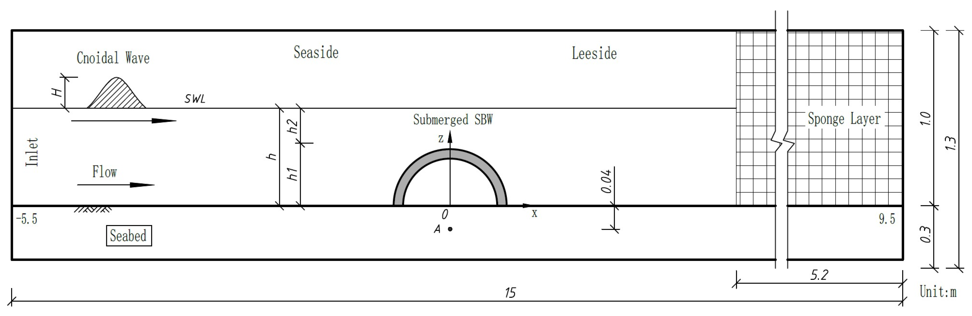
3.2. Numerical Setup

The sketch of the numerical layout is depicted in Figure 5, where the scale is 1:25. Figure 6 illustrates the characteristics of perforated SBWs. Previous studies have shown that dividing the waveform into 20 grids within the wave height range provides a more accurate representation [31,32]. To discretize the domain, a total of 800,000 cells are used. The first block comprises 500,000 cells, with dimensions of 0.03 m, while the second block comprises 300,000 cells, with dimensions of 0.01 m. Initial simulations are conducted using various grid resolutions to achieve an adequate solution in terms of capturing the relevant flow details.

The wave and the current are generated at the inlet boundary. The renormalized group (RNG) turbulence model is used to represent turbulent flow phenomena. To reduce wave reflection from the boundary, a wave-absorbing layer is installed ahead of the outflow boundary. The bottom of the domain is designated as a wall boundary type, while the other boundaries are set as symmetry types. The time ranges from 0 s to 20 s, with intervals of 0.0475 s.

The type of incident wave in cases of wave–current interaction is determined by the wave height (H), period (T), water depth (d), and flow velocity (c). In the nearshore of West Africa, the interaction between waves and currents is particularly significant, intensifying the dynamic response of the seabed. This study uses hydrographic data from the fishing port in Ghana, West Africa, as presented in

Table 2. Index properties of wave and breakwater structures.

Cases	Flow Velocity (m/s)	Wave Height (m)	Water Depth (m)	Wave Period (s)	Perforation Rate (n)	Perforation Number (i)	Perforation Type
1	0.08	0.060	0.228	1.9	10%	7	Basic perforation
2	0.08	0.088	0.228	1.9	10%	7	Basic perforation
3	0.08	0.100	0.228	1.9	10%	7	Basic perforation
4	0.08	0.088	0.228	1.9	10%	7	Basic perforation
5	0.08	0.088	0.292	1.9	10%	7	Basic perforation
6	0.08	0.088	0.312	1.9	10%	7	Basic perforation
7	0.08	0.088	0.228	1.6	10%	7	Basic perforation
8	0.08	0.088	0.228	1.9	10%	7	Basic perforation
9	0.08	0.088	0.228	2.2	10%	7	Basic perforation
10	0.08	0.088	0.228	1.9	5%	7	Basic perforation
11	0.08	0.088	0.228	1.9	10%	7	Basic perforation
12	0.08	0.088	0.228	1.9	15%	7	Basic perforation
13	0.08	0.088	0.228	1.9	10%	3	Basic perforation
14	0.08	0.088	0.228	1.9	10%	5	Basic perforation
15	0.08	0.088	0.228	1.9	10%	7	Basic perforation
16	0.08	0.088	0.228	1.9	10%	3	Front perforation
17	0.08	0.088	0.228	1.9	10%	7	Basic perforation
18	0.08	0.088	0.228	1.9	10%	7	Rear perforation

. The liquefaction criteria [33] used in this study are outlined as follows:

$$-{\mathsf{\sigma }}_{\mathrm{z}0}⩽\mathrm{p}-{\mathrm{p}}_{\mathrm{b}}$$

(13)

where p_b is the excess pore water pressure (wave dynamic pressure), (p − p_b) is the excess pore water pressure difference, and ${\mathsf{\sigma }}_{\mathrm{z}0}$ is the initial effective stress of the soil.

4. Results and Discussion

In this section, the effects of marine environments and breakwater structures on the seabed dynamic response are investigated.

4.1. Impact of the Marine Environment

In the ocean, the marine environment is diverse. This section analyzes the impact of the wave height, water depth, and wave period on the seabed response. The perforation rate is 10%, the perforation number is 7, and the perforation type is basic perforation. The liquefaction depths of the seabed in different marine environments are detailed in

Table 3. Liquefaction depths in different marine environments.

Cases	Flow Velocity (m/s)	Wave Height (m)	Water Depth (m)	Wave Period (s)	Maximum Liquefaction Depth in the Seaside (cm)	Maximum Liquefaction Depth in the Leeside (cm)	Average Liquefaction Depth (cm)
1	0.08	0.060	0.228	1.9	1.22	0.07	0.18
2	0.08	0.088	0.228	1.9	2.74	0.14	0.63
3	0.08	0.100	0.228	1.9	3.02	0.30	0.82
4	0.08	0.088	0.228	1.9	2.74	0.14	0.63
5	0.08	0.088	0.292	1.9	2.69	0.08	0.70
6	0.08	0.088	0.312	1.9	2.47	0.06	0.65
7	0.08	0.088	0.228	1.6	2.55	0.51	0.90
8	0.08	0.088	0.228	1.9	2.76	0.71	1.06
9	0.08	0.088	0.228	2.2	2.85	0.90	1.30

.

4.1.1. Wave Height

Figure 7 shows the maximum pore pressure and liquefaction depth for different wave heights. As the wave height increases, the maximum pore pressure at the same seabed depth also increases, especially within the range of −0.3 < z/h < 0. This increase is due to the intensified hydrodynamic forces acting on the seabed, resulting in higher pore pressure. Within the range of −1 < z/h < −0.3, there is a noticeable reduction in the rate of pore pressure dissipation, causing a gradual decrease in pore pressure toward 0 Pa. This phenomenon explains why the seabed in shallow regions is prone to experiencing transient liquefaction.

Figure 7b illustrates that the range of seabed liquefaction is within 0.05 m and correlates positively with changes in wave height. Due to wave reflection by the SBW, the maximum liquefaction depth typically occurs in the seaside [18]. With an increase in wave height from 0.06 m to 0.10 m, the maximum liquefaction depth increases from 1.22 cm to 3.02 cm.

4.1.2. Water Depth

Figure 8 illustrates the dynamic response of the seabed to different wave depths. With increasing water depth, the energy transmitted to the seabed surface indirectly decreases, leading to a reduced dynamic response of the seabed. The impact of water depth on liquefaction is weak, with only a slight decrease, of 0.27 cm observed in the liquefaction depth in the seaside. No significant changes are observed in the liquefaction depth in the leeside or in the overall average liquefaction depth.

4.1.3. Wave Period

Figure 9 illustrates the seabed response to different wave periods. As the wave period increases, the wave energy strengthens, resulting in a slight increase in the pore pressure around the SBW. Moreover, a notable increase in liquefaction depth occurs. This phenomenon is caused by the increased wave transmission associated with longer periods, intensifying wave action in the leeside, consistent with previous studies [34]. Specifically, leeside liquefaction increases by 0.39 cm, with the average liquefaction depth increasing by 0.4 cm. The analysis demonstrates that pore pressure increases significantly, leading to seabed liquefaction under the influence of long-period waves. This poses a substantial threat to the stability of the seabed. The liquefaction characteristic values of the seabed in different marine environments can be found in Table 3.

4.2. Impact of Breakwater Structure

In this section, the effects of the perforation rate, perforation number, and perforation type on hydrodynamic response characteristics and the seabed dynamic response are analyzed. The flow velocity is 0.08 m/s, the wave height is 0.088 m, the water depth is 0.228 m, and the wave period is 1.9 s.

Figure 10 depicts the velocity contour in the flow field at different time points: 9.07 s, 9.30 s, 10.17 s, and 10.64 s. When the wave crest is above the SBW (t = 9.07 s), significant wave transformation occurs above the breakwater, leading to the maximum velocity. As the wave traverses the breakwater at 9.30 s, the flow velocity surrounding the structure decreases, resulting in the expansion of the core vortex. An inverse head is observed, with the water level in the leeside surpassing that in the seaside. The development of a reverse flow leads to intensified water mixing and the formation of multiple high-intensity vortices by 10.17 s. By 10.64 s, the approaching wave causes incident and recirculating waters to mix within the arch, contributing to wave energy dissipation. This process illustrates the primary mechanism for energy dissipation in the SBW.

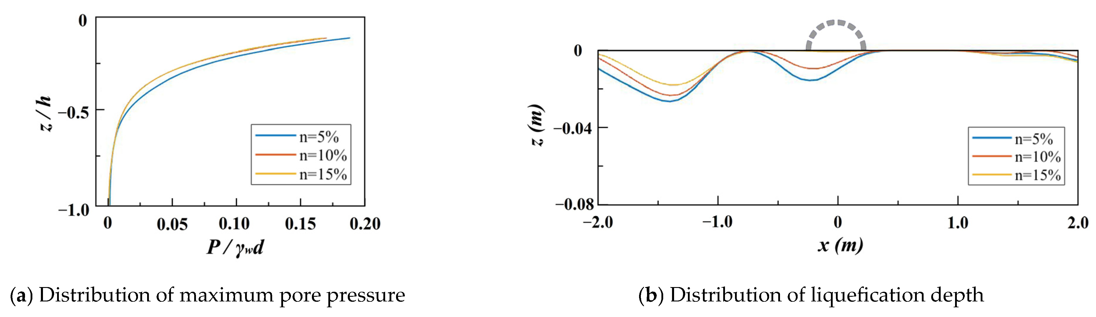
4.2.1. Breakwater Perforation Rate

Figure 11 compares the velocity contours at the wave crest and the wave trough at different perforation rates. The perforated SBW creates a stilling chamber due to its structure. As the perforation rate increases, the flow velocity decreases above the breakwater, while increasing inside the breakwater. This occurs because the effective water-blocking area decreases significantly, allowing water to enter and exit more easily through the structure. At a perforation rate of 15%, excessive perforations reduce disturbance levels, leading to a notable reduction in vortices and the turbulence intensity within the arch. As the reverse flow develops, the increasing perforation rate reduces the extent of the reverse head due to expanded water flow paths. This diminishes the range of vortices within the arch, weakening their impact on the seabed. Additionally, perforations with the minimum internal cross-section area consistently exhibit higher flow velocities in the region.

Figure 12 illustrates that increasing the perforation rate results in a reduced liquefaction depth. Increasing the perforation rate from 5% to 10% reduces the turbulent intensity within the arch, resulting in a 17.3% decrease in the average seabed liquefaction depth. A perforation rate of 15% results in minimal liquefaction around the SBW, with a 23.2% decrease in the liquefaction depth in the seaside. These findings are consistent with previous studies indicating that wave transmission increases with higher perforation rates [4,34,35]. This study proposes the existence of an optimal perforation rate that maximizes the wave dissipation capacity, while ensuring seabed stability.

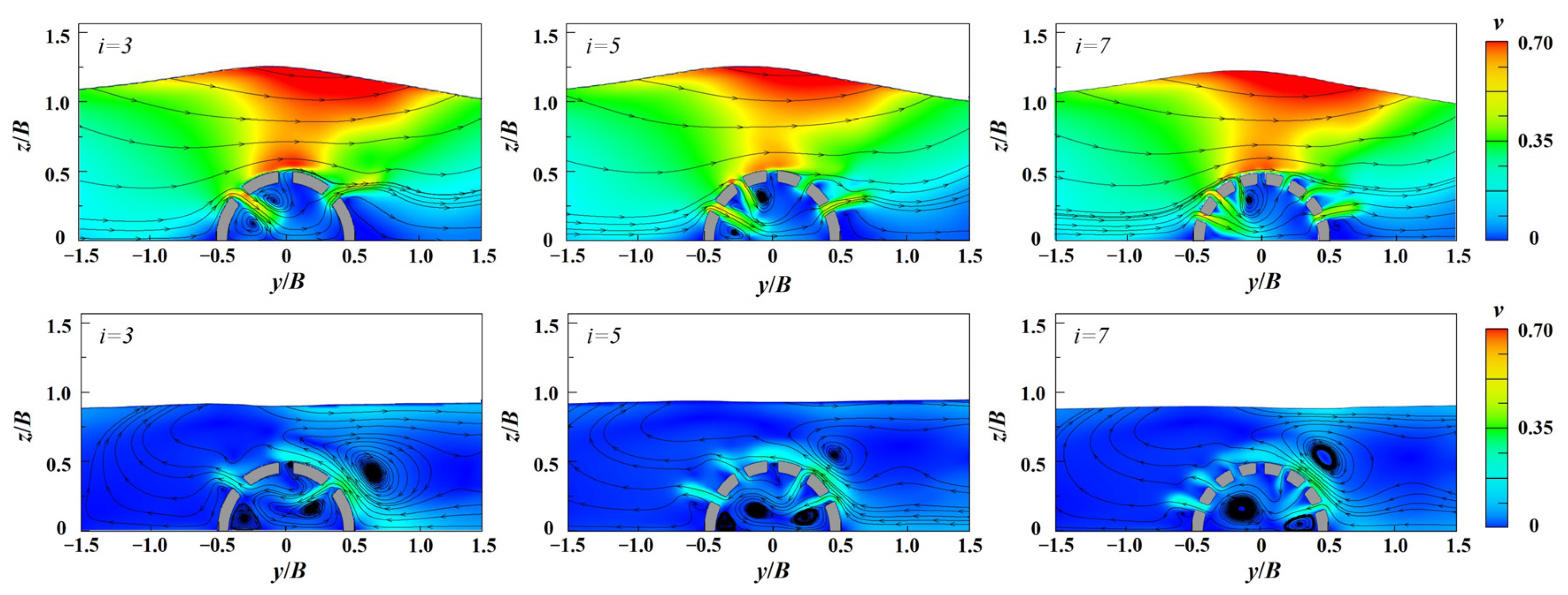
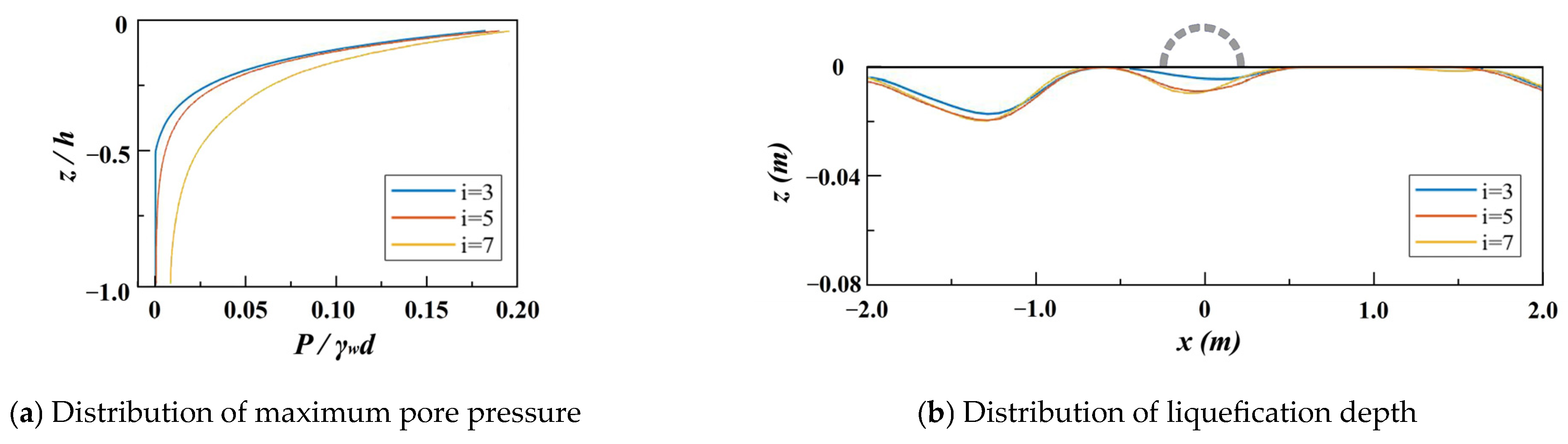
4.2.2. Breakwater Perforation Number

Figure 13 depicts the velocity contours of the flow fields around the SBW with different perforation numbers. Initially, as the perforation number increases, there is a decrease in flow velocity, followed by an increase. This phenomenon occurs because the increased number of pathways for water flow initially reduces flow velocity. Simultaneously, a significant velocity gradient within the arch enhances water mixing due to the influence of reverse flow. However, as the perforation number continues to increase, the decrease in the perforation rate limits the water drainage capacity. Overflowing water over the top of the breakwater not only increases flow velocity but also strengthens the inverse head, leading to expanded vortices within the arch.

Figure 14 illustrates the increase in pore pressure with an increasing perforation number. However, the influence of the perforation number on seabed liquefaction is relatively minor. An increase in the perforation number results in an approximate 8% increase in liquefaction in the seaside, along with a decrease in liquefaction in the leeside. When the perforation number is 3, the reduced presence of vortices significantly mitigates the seabed liquefaction.

4.2.3. Breakwater Perforation Type

Figure 15 illustrates the velocity contours of flow fields for different perforation types. On the one hand, basic perforation allows water to pass through more easily, leading to a more stable flow field and improved seabed stability, as demonstrated in Figure 16. Moreover, basic perforation exhibits strong wave transmission properties and is less susceptible to reverse water flow [4]. This reduction significantly minimizes flow field disturbances and increases structural stresses. Sasajima et al. [36] noted that the wave dissipation effect of basic perforation is relatively weak due to the low intensity of wave dissipation vortices.

On the other hand, front and rear perforations rely on one-sided drainage, affecting flow uniformity and water pressure gradients. This influences flow field stability and exacerbates local seabed responses (as shown in Figure 16). The seaside liquefaction for the front perforation increases by 22.9% and the leeside liquefaction for the rear perforation increases by 45.9% compared to the basic perforation. The increased local flow velocity leads to increased disturbances on the seabed. Thus, it is important to account for these factors when designing structures to withstand such impacts and disturbances, ensuring the stability and safety of SBWs. The liquefaction characteristic values of different breakwater structures are detailed in

Table 4. Liquefaction depths of different breakwater structures.

Cases	Perforation Rate (n)	Perforation Number (i)	Perforation Type	Maximum Liquefaction Depth in the Seaside (cm)	Maximum Liquefaction Depth in the Leeside (cm)	Average Liquefaction Depth (cm)
10	5%	7	Basic perforation	2.64	0.58	0.75
11	10%	7	Basic perforation	2.33	0.37	0.54
12	15%	7	Basic perforation	1.79	0.27	0.37
13	10%	3	Basic perforation	1.65	0.85	0.53
14	10%	5	Basic perforation	1.78	0.79	0.61
15	10%	7	Basic perforation	1.92	0.64	0.69
16	10%	3	Front perforation	2.49	0.46	0.90
17	10%	7	Basic perforation	1.92	0.64	0.69
18	10%	7	Rear perforation	1.90	1.11	1.01

.

5. Conclusions

This study numerically investigates the effects of marine environments and breakwater structures on seabed dynamic responses. Specifically, it investigates the influence of waves with varying wave heights, water depths, and wave periods. The structural characteristics, including the perforation rate, perforation number, and perforation type, are considered to meet the construction requirements of SBWs. The main conclusions are as follows:

• The model developed in this study is well suited for investigating the dynamic response of the seabed. The wave model accurately simulates wave generation, propagation, and reflection processes. Additionally, the seabed model effectively captures liquefaction in the seabed foundation.
• Wave characteristics significantly influence the dynamic response of the seabed. Pore pressure and liquefaction show a positive correlation with wave height and wave period, while exhibiting a negative correlation with water depth.
• The perforation rate of the SBW has a minor effect on pore pressure. Increasing the perforation rate from 5% to 10% leads to a 32% decrease in the average liquefaction depth. The increasing perforation number slightly enhances pore pressure and deepens liquefaction due to complex wave reflection and transmission. Among the three different perforation types, basic perforation exerts the minimum seabed pressure. Front perforation increases liquefaction by 22.9% in the seaside, and rear perforation increases liquefaction by 45.9% in the leeside.
• In the design of SBWs, it is crucial to consider both wave dissipation and the stability of seabed liquefaction comprehensively. Measures such as reducing the permeability of the seabed can be implementing to enhance the stability of the seabed soil.

References

1. Tanimoto, K.; Takahashi, S. Design and construction of caisson breakwaters—The Japanese experience. Coast. Eng. 1994, 22, 57–77. [Google Scholar] [CrossRef]
2. Xie, S. Waves forces on submerged semicircular breakwater and similar structures. China Ocean Eng. 1999, 13, 63–72. [Google Scholar]
3. Liu, Y.; Li, H.-J. Analysis of wave interaction with submerged perforated semi-circular breakwaters through multipole method. Appl. Ocean Res. 2012, 34, 164–172. [Google Scholar] [CrossRef]
4. Dhinakaran, G.; Sundar, V.; Sundaravadivelu, R.; Graw, K. Dynamic pressures and forces exerted on impermeable and seaside perforated semicircular breakwaters due to regular waves. Ocean Eng. 2002, 29, 1981–2004. [Google Scholar] [CrossRef]
5. Guo, L.; Cai, Y.; Jardine, R.J.; Yang, Z.; Wang, J. Undrained behaviour of intact soft clay under cyclic paths that match vehicle loading conditions. Can. Geotech. J. 2018, 55, 90–106. [Google Scholar] [CrossRef]
6. Wang, Y.-Z.; Yan, Z.; Wang, Y.-C. Numerical analyses of caisson breakwaters on soft foundations under wave cyclic loading. China Ocean Eng. 2016, 30, 1–18. [Google Scholar] [CrossRef]
7. Hu, C.; Liu, H.; Huang, W. Anisotropic bounding-surface plasticity model for the cyclic shakedown and degradation of saturated clay. Comput. Geotech. 2012, 44, 34–47. [Google Scholar] [CrossRef]
8. Mynett, A.E.; Mei, C. Wave-induced stresses in a saturated poro-elastic sea bed beneath a rectangular caisson. Geotechnique 1982, 32, 235–247. [Google Scholar] [CrossRef]
9. Tsai, Y.; McDougal, W.; Sollitt, C. Response of finite depth seabed to waves and caisson motion. J. Waterw. Port Coast. Ocean. Eng. 1990, 116, 1–20. [Google Scholar] [CrossRef]
10. Mase, H.; Sakai, T.; Sakamoto, M. Wave-induced porewater pressures and effective stresses around breakwater. Ocean Eng. 1994, 21, 361–379. [Google Scholar] [CrossRef]
11. Jeng, D.; Cha, D.; Lin, Y.; Hu, P. Analysis on pore pressure in an anisotropic seabed in the vicinity of a caisson. Appl. Ocean Res. 2000, 22, 317–329. [Google Scholar] [CrossRef]
12. Jeng, D.; Cha, D.; Lin, Y.; Hu, P. Wave-induced pore pressure around a composite breakwater. Ocean Eng. 2001, 28, 1413–1435. [Google Scholar] [CrossRef]
13. Zhang, J.-S.; Jeng, D.-S.; Liu, P.-F. Numerical study for waves propagating over a porous seabed around a submerged permeable breakwater: PORO-WSSI II model. Ocean Eng. 2011, 38, 954–966. [Google Scholar] [CrossRef]
14. Zhang, Y.; Zhang, J.; Zhang, H.; Zhao, H.; Jeng, D. Three-dimensional model for wave-induced dynamic soil response around breakwaters. In Proceedings of the 22nd International Offshore and Polar Engineering Conference, Rhodes, Greece, 17–23 June 2012; ISOPE: Mountain View, CA, USA, 2012. [Google Scholar]
15. Zhao, H.Y.; Jeng, D.S.; Zhang, Y.; Zhang, J.S.; Zhang, H.J.; Zhang, C. 3D numerical model for wave-induced seabed response around breakwater heads. Geomech. Eng. 2013, 5, 595–611. [Google Scholar] [CrossRef]
16. Mizutani, N.; McDougal, W.; Mostafa, A. BEM-FEM combined analysis of nonlinear interaction between wave and submerged breakwater. In Coastal Engineering 1996, Proceedings of the Twenty-fifth International Conference, Orlando, FL, USA, 2–6 September 1996; American Society of Civil Engineers: Reston, VA, USA, 1997; pp. 2377–2390. [Google Scholar]
17. Mostafa, A.M.; Mizutani, N.; Iwata, K. Nonlinear wave, composite breakwater, and seabed dynamic interaction. J. Waterw. Port Coast. Ocean. Eng. 1999, 125, 88–97. [Google Scholar] [CrossRef]
18. Yan, Z.; Zhang, H.; Sun, X. Tests on wave-induced dynamic response and instability of silty clay seabeds around a semi-circular breakwater. Appl. Ocean Res. 2018, 78, 1–13. [Google Scholar] [CrossRef]
19. Vastenholz, H. The Interdependent Effects of Wave Reflection and Seabed Erosion. In Proceedings of the 3rd International Conference on Scour and Erosion (ICSE-3), Amsterdam, The Netherlands, 1–3 November 2006; CURNET: Gouda, The Netherlands, 2006; pp. 669–674. [Google Scholar]
20. Xu, W.; Chen, C.; Htet, M.H.; Sarkar, M.S.I.; Tao, A.; Wang, Z.; Fan, J.; Jiang, D. Experimental Investigation on Bragg Resonant Reflection of Waves by Porous Submerged Breakwaters on a Horizontal Seabed. Water 2022, 14, 2682. [Google Scholar] [CrossRef]
21. Brunone, B.; Tomasicchio, G.R. Wave kinematics at steep slopes: Second-order model. J. Waterw. Port Coast. Ocean Eng. 1997, 123, 223–232. [Google Scholar] [CrossRef]
22. Yakhot, V.; Orszag, S.A. Renormalization group analysis of turbulence. I. Basic Theory. J. Sci. Comput. 1986, 1, 3–51. [Google Scholar] [CrossRef]
23. Yakhot, V.; Smith, L.M. The renormalization group, the ε-expansion and derivation of turbulence models. J. Sci. Comput. 1992, 7, 35–61. [Google Scholar] [CrossRef]
24. Hirt, C.W.; Nichols, B.D. Volume of fluid (VOF) method for the dynamics of free boundaries. J. Comput. Phys. 1981, 39, 201–225. [Google Scholar] [CrossRef]
25. Biot, M.A. Theory of propagation of elastic waves in a fluid-saturated porous solid. II. Higher frequency range. J. Acoust. Soc. Am. 1956, 28, 179–191. [Google Scholar] [CrossRef]
26. Zienkiewicz, O.; Chang, C.; Bettess, P. Drained, undrained, consolidating and dynamic behaviour assumptions in soils. Geotechnique 1980, 30, 385–395. [Google Scholar] [CrossRef]
27. Sui, T.; Zhang, C.; Guo, Y.; Zheng, J.; Jeng, D.; Zhang, J.; Zhang, W. Three-dimensional numerical model for wave-induced seabed response around mono-pile. Ships Offshore Struct. 2016, 11, 667–678. [Google Scholar] [CrossRef]
28. Sui, T.; Zheng, J.; Zhang, C.; Jeng, D.S.; Zhang, J.; Guo, Y.; He, R. Consolidation of unsaturated seabed around an inserted pile foundation and its effects on the wave-induced momentary liquefaction. Ocean Eng. 2017, 131, 308–321. [Google Scholar] [CrossRef]
29. Mizutani, N.; Mostafa, A.M. Nonlinear wave-induced seabed instability around coastal structures. Coast. Eng. J. 1998, 40, 131–160. [Google Scholar] [CrossRef]
30. Wu, Y.-T.; Hsiao, S.-C. Propagation of solitary waves over a submerged permeable breakwater. Coast. Eng. 2013, 81, 1–18. [Google Scholar] [CrossRef]
31. Deng, B.; Yin, L.; Huang, J.; Xiong, K.; Jiang, C. Three dimensional numerical simulation of wave interaction with a new type of double row perforated cylinder breakwater. Chin. J. Theor. Appl. Mech. 2023, 55, 845–857. [Google Scholar]
32. Zhang, T. Three-Dimensional Numerical Simulation of Waves and Its Application. Master’s Thesis, Tianjin University, Tianjin, China, 2009. [Google Scholar]
33. Ye, J. 3D liquefaction criteria for seabed considering the cohesion and friction of soil. Appl. Ocean Res. 2012, 37, 111–119. [Google Scholar] [CrossRef]
34. Pan, T.; Feng, X.; Ni, X.; Feng, W.; Ma, G. Study on the response of wave transmission coefficient to various incident wave elements of a permeable sloping breakwater. J. Hohai Univ. (Nat. Sci.) 2022, 50, 45–53. [Google Scholar]
35. Teh, H.M. Wave Transmission over a Submerged Porous Breakwater: An Experimental Study. In Proceedings of the 2nd International Conference on Civil, Offshore and Environmental Engineering (ICCOEE), Kuala Lumpur, Malaysia, 3–5 June 2014. [Google Scholar]
36. Sasajima, H. Field demonstration test on a semi-circular breakwater. In HYDRO-PORT’94, Proceedings of the International Conference on Hydro-Technical Engineering for Port and Harbor Construction, Yokosuka, Japan, 19–21 October 1994; Coastal Development Institute of Technology: Tokyo, Japan, 1994. [Google Scholar]
Figure 1. Sketch of the validation simulation setup for wave interaction.
Jmse 12 00873 g001
Figure 2. Comparison of the pore pressure between experimental and numerical simulations.
Jmse 12 00873 g002
Figure 3. Comparison of the waveforms of experimental and numerical water surfaces.
Jmse 12 00873 g003
Figure 4. Comparison of the horizontal and vertical velocities of experimental and numerical results.
Jmse 12 00873 g004
Figure 5. Sketch of the simulation setup for wave interaction with a perforated SBW (not to scale).
Jmse 12 00873 g005
Figure 6. Sketches of different SBW structures.
Jmse 12 00873 g006
Figure 7. Distribution of the seabed response for different wave heights. (The gray half circle represents the location of the semi-circular breakwater).
Jmse 12 00873 g007
Figure 8. Distribution of the seabed response for different water depths. (The gray half circle represents the location of the semi-circular breakwater).
Jmse 12 00873 g008
Figure 9. Distribution of the seabed response for different wave periods. (The gray half circle represents the location of the semi-circular breakwater).
Jmse 12 00873 g009
Figure 10. Velocity contours around the SBW with different phases. (Arrows indicate the flow direction; The gray half circle represents the location of the semi-circular breakwater).
Jmse 12 00873 g010
Figure 11. Velocity contours around the SBW at different perforation rates. (Arrows indicate the flow direction; The gray half circle represents the location of the semi-circular breakwater).
Jmse 12 00873 g011
Figure 12. Distribution of the seabed response at different perforation rates. (The gray half circle represents the location of the semi-circular breakwater).
Jmse 12 00873 g012
Figure 13. Velocity contours around the SBW at different perforation numbers. (Arrows indicate the flow direction; The gray half circle represents the location of the semi-circular breakwater).
Jmse 12 00873 g013
Figure 14. Distribution of the seabed response at different perforation numbers. (The gray half circle represents the location of the semi-circular breakwater).
Jmse 12 00873 g014
Figure 15. Velocity contours around the SBW with different perforation types. (Arrows indicate the flow direction; The gray half circle represents the location of the semi-circular breakwater).
Jmse 12 00873 g015
Figure 16. Distribution of the seabed response with different perforation types. (The gray half circle represents the location of the semi-circular breakwater).
Jmse 12 00873 g016