Analysis of Wind Energy Potential in Sri Lankan Waters Based on ERA5 (ECMWF Reanalysis v5) and CCMP (Cross-Calibrated Multi-Platform)

Abstract

Amid global energy demands and environmental concerns, the exploration of renewable energy sources has become critically important. This study presents a comprehensive analysis of wind energy dynamics over a 35-year period (1988–2022) using CCMP and ERA5 datasets. It focuses on the spatial and temporal characteristics of wind energy within the region, particularly its distribution. The wind field in Sri Lanka has significant seasonal and regional characteristics. Despite seasonal variations, the overall wind activity remains moderate, with speeds generally above 5.4 m/s and annual average wind power densities exceeding 150 W/m², reaching up to 200 W/m² in certain areas. The two primary wind directions in the waters near Sri Lanka are WSW and NE. The study identifies periods of high stability, particularly from June to August, where effective wind speed occurrence (EWSO) exceeds 80%. A ‘W’-shaped pattern in monthly variations corresponds with changes in wind power density (WPD), highlighting optimal periods for wind energy extraction. Additionally, estimated reserves and technically exploitable wind energy resources (WERs) suggest that wind energy development off Sri Lanka is feasible, with potential capacities of approximately 2.00 GW and 1.60 GW, respectively. The overall coefficient of variation (CV) is small, indicating stable wind energy conditions. This analysis not only provides a scientific basis for evaluating WERs near Sri Lanka but also offers valuable insights for strategic planning and development in the renewable energy sector.

1. Introduction

Considering the tremendous development in global energy demand and the increasing negative impact of traditional fossil fuels on the environment, the development and application of sustainable energy sources have become the key to solving the global energy crisis and environmental problems. Studies have shown that the extensive use of fossil fuels in the energy supply is one of the main causes of climate change and poses a serious threat to public health. To lessen the dependence on fossil fuels for power generation, many countries around the world are gradually transitioning to renewable energy and implementing a series of progressive energy policies aimed at reducing environmental pollution and promoting sustainable development [1].

Among the various sustainable energy sources, wind energy is a major source of electricity due to its proven technology, commercial viability, and relatively low CO₂ emissions [2]. It is estimated that by 2050, wind power generation will meet a quarter to a third of global electricity demand [3]. Therefore, a thorough analysis of wind energy potential is critical for effective wind energy resources (WERs) development and exploitation.

Several methods are used to analyze wind energy potential, including observation-based analysis [4], satellite remote sensing analysis [5,6,7], model-based analysis [8,9], and reanalysis data-based analysis [10,11]. Recently, the study of wind energy potential with artificial neural network-based models has received attention [12].

As available resources on land dwindle, many countries around the world are turning their attention to the potential of offshore wind energy. Studies have shown that compared to land, offshore WS may be as high as 8.60 m/s (WS at level 6) at 80 m above sea level, compared to only 4.54 m/s (WS at level 1) on land [13]. The global ocean is abundant with WERs and the potential power of offshore wind power is as high as 39 TW, which is 54% of the global total [14]. As a result, the global ocean is considered to be crucial for the growth of WERs; furthermore, global future WERs show a good trend for offshore wind energy [15,16,17].

The Indian Ocean, significantly influenced by the monsoon, presents a sea area with high research and application value for analyzing wind energy resource potential. Previous studies have indicated that from 1979 to 2015, the northern Indian Ocean was rich in WERs across most of its area, showing significant growth trends or stability [18]. Research on the shelf seas off the south coast of India has revealed abundant WERs, with particularly high potential for wind power generation during the summer months [19,20,21,22]. The annual demand for electrical power in Sri Lanka has been increasing at a rate of 7~8%. This trend is predicted to continue, underscoring the crucial role of developing WERs to sustainably meet the increasing energy demand [23].

Despite previous studies on offshore wind power in Sri Lanka, a precise and thorough evaluation of WERs in the area has not been possible due to insufficient measured data. This study aims to comprehensively and systematically analyze the wind energy potential in the sea adjacent to Sri Lanka using the CCMP (Cross-Calibrated Multi-Platform) and ERA5 datasets to fill the gaps in existing studies and to offer a scientific foundation and guidance for future wind energy development endeavors. Additionally, by comparing the findings of prior studies with those of this research, we aim to provide more precise and comprehensive information for medium- and long-term planning and strategy development for wind energy development.

2. Study Area and Data

2.1. Study Area

This investigation aims to assess the potential for wind energy generation along the coast of Sri Lanka. Situated in the Indian Ocean, Sri Lanka is an island nation located between latitudes 5.91° N and 9.83° N, and longitudes 79.70° E and 81.88° E. To comprehensively analyze the distribution of WERs in this area, we expanded the study area to cover a wider region spanning from 3° N to 13° N latitude and 75° E to 85° E longitude. This area is subject to significant seasonal variations: the southwest monsoon primarily affects the weather between June and August, whereas the northeast monsoon prevails from December to February. These monsoons provide unique geographic and climatic conditions critical for assessing WERs. Figure 1 shows the location of the study area and observation site.

2.2. Data Presentation

2.2.1. CCMP (Cross-Calibrated Multi-Platform)

The CCMP wind field information is generated by synthesizing sea surface wind field data obtained from satellite microwave remote sensing and ground-based observational instruments, which are processed using cross-calibration and data assimilation techniques (http://data.remss.com/, accessed on 9 September 2023). This synthetic wind field information is presented at a spatial resolution of 0.25° × 0.25° and a temporal resolution of 6 h, covering a 35-year time span from 1 January 1988 to 31 December 2022. The data comprise u and v wind field components at a height of 10 m, offering wind data across a broad spectrum of temporal and spatial scales. The u and v typically represent the eastward and northward components of wind vectors.

2.2.2. ERA5 (ECMWF Reanalysis 5)

The ERA5 reanalysis data are sourced from the European Center for Medium-Range Weather Forecasts (ECMWF) and are derived using the ECMWF’s Integrated Forecasting System IFS (CY41R2) (https://cds.climate.copernicus.eu/, accessed on 9 September 2023). ERA5 offers global meteorological data from 1979 to the present day. For this study, data spanning from 1 January 1988 to 31 December 2022 were chosen. The dataset features a spatial resolution of 0.25° and is updated hourly with high temporal resolution, with a specific focus on WS data at 10 m above sea level.

2.2.3. Measured Observation Data

This study also referred to the Sri Lankan flux tower observation data provided by the China-Sri Lanka Joint Center for Education & Research of the Chinese Academy of Sciences (CAS). The observatory is located at Ruhuna in the southern part of Sri Lanka, with specific coordinates of 80.5779° E and 5.9357° N, at approximately 10 m above sea level. The data were collected from 10 April 2017 to 3 September 2018 as hourly updated WS and direction data, which provided valuable ground-truth measurements to validate and calibrate the remotely sensed and reanalyzed information for this study.

2.3. Data Validation

To ensure the accuracy and reliability of the CCMP and ERA5 wind field data used in the study, this paper analyzes these two data in comparison with the measured data from the Sri Lankan flux tower. The comparison methodology includes the use of six statistical metrics: correlation coefficient ($r$), root mean square error ($RMSE$), average error ($AE$), average absolute deviation ($AAE$), reliability index ($RI$) and model efficiency factor ($MEF$) [24]. These metrics provide us with a comprehensive assessment framework to quantify the differences between model predictions and measured data and their correlations. The correlation calculation formula is shown below:

$$r=\frac{{\sum }_{i=1}^n(O_i-\overline{O})(P_i-\overline{P})}{\sqrt{{\sum }_{i=1}^n{(O_i-\overline{O})}^2{\sum }_{i=1}^n{(P_i-\overline{P})}^2}}$$

(1)

$$RMSE=\sqrt{\frac{{\sum }_{i=1}^n{(P_i-O_i)}^2}{n}}$$

(2)

$$AE=\frac{{\sum }_{i=1}^n(P_i-O_i)}{n}=\overline{P}-\overline{O }$$

(3)

$$AAE=\frac{{\sum }_{i=1}^n\left|P_i-O_i\right|}{n}$$

(4)

$$RI=exp\sqrt{\frac{1}{n}{\displaystyle \sum _{i=1}^n}{\left(\log \frac{O_i}{P_i}\right)}^2}$$

(5)

$$MEF=\frac{{\sum }_{i=1}^n{(O_i-\overline{O})}^2-{\sum }_{i=1}^n{(P_i-O_i)}^2}{{\sum }_{i=1}^n{(O_i-\overline{O})}^2}$$

(6)

where $n$ represents the number of observations, $O_i$ represents the $i$-th observation out of $n$, $P_i$ represents the $i$-th forecast out of $n$, and $\overline{O}$ and $\overline{P}$ denote the averages of observations and forecasts, respectively.

Correlation coefficient ($r$) measures the strength and direction of the linear relationship between predicted and observed values. The coefficient ranges from −1 to 1. A value closer to 1 or −1 indicates a stronger linear relationship between the prediction and the actual observation, while a value closer to 0 indicates a weaker linear relationship between the two.

RMSE measures the overall difference between predicted and measured values, giving higher weight to larger errors, so that lower RMSE values indicate better prediction accuracy.

AE represents the mean difference between predicted and measured values, indicating the typical deviation of predicted values from observed values. Positive values indicate that predicted values are typically higher than observed values, while negative values indicate that predicted values are typically lower than observed values.

AAE measures the average absolute difference between individual predicted values and observed values. Smaller AAE values indicate lower prediction errors and better prediction performance of the model.

RI is a metric that quantifies the magnitude of the average difference between predicted and observed values, derived from the log-transformed root-mean-square error between predicted and observed values [25]. Ideally, an RI value close to 1 indicates a high degree of predictive reliability.

A value of MEF close to 1 indicates good model performance, meaning that the model’s predictive power is better than a baseline model that simply uses the observed mean as a predictor. A value of MEF below 0 indicates that the model’s predictive power is not as good as the observed mean.

Table 1. Computed error statistics based on flux tower data for CCMP and ERA5, respectively.

	Hourly Wind Speed and Direction Data from 10 April 2017 to 3 September 2018
	CCMP	ERA5
n	1998	1998
r	0.579398	−0.22774
RMSE	1.940097	2.204041
RI	1.740111	1.939713
AE	1.461046	0.449316
AAE	1.557906	1.768546
MEF	−1.30285	−1.97206

presents the six statistical metrics derived from flux tower data for CCMP and ERA5. The comparative analysis between CCMP and ERA5 wind field datasets against in situ measurements reveals a significant correlation with the CCMP data (r = 0.579), suggesting a more accurate reflection of actual WS trends by the CCMP dataset. Additionally, the CCMP data outperform ERA5 in terms of root-mean-square error, mean error, and mean absolute error, highlighting its superior accuracy in modeling wind speeds in the maritime zone off Sri Lanka. Despite the CCMP wind speed values being marginally lower, their overall consistency with the measured values substantiates the dataset’s reliability.

3. Introduction to the Research Methodology

3.1. EOF Analysis

Empirical Orthogonal Function (EOF) analysis is a widely used statistical tool for extracting principal data characteristics, especially in meteorology, oceanography, and climate science. It was initially proposed by statistician Pearson in 1902, and Lorenz first introduced it to weather and climate research in the nineteen fifties [26,27]. It simplifies complex datasets by breaking them down into a series of orthogonal functions, efficiently concentrating original information within the first few modes while retaining significant physical meaning. The resulting eigenvalues from this decomposition offer a quantitative measure of each factor’s spatial distribution characteristics and variance degree.

The basic principle of EOF analysis is to obtain a set of orthogonal eigenvectors (EOF patterns) and corresponding eigenvalues by eigenvalue decomposition of the covariance matrix or correlation matrix of a data set. Each EOF pattern is an independent representation of the variance in the dataset, while the magnitude of the eigenvalue reflects the proportion of the pattern in the total variance of the dataset. By analyzing the first few major EOF patterns, the main variation patterns in the data and their spatial distribution characteristics can be identified. For such a spatiotemporal dataset of a meteorological variable, comprising m spatial points (x₁, x₂, …, x_m) and n time points (t₁, t₂, …, t_n), we can represent it using a matrix $X_{m\times n}$ of size mxn.

The specific algorithm is described below:

(1) Selected data, processed into distance flats to obtain the data matrix ${ X}_{m\times n}$.

(2) Find the cross product of $X$ with $X^T$ to obtain the following square matrix.

$$C_{m\times m}=\frac{1}{\mathrm{n}}X\times X^T$$

(7)

(3) Calculate the eigenvalues and eigenvectors $v_{m\times m}$ of $C_{m\times m}$, where both satisfy the conditions:

$$C_{m\times m}\times V_{m\times m}=V_{m\times m}\times E_{m\times m}$$

(8)

$$E=\left[\begin{array}{cccc}{\lambda }_1& 0& \cdots & 0\\ 0& {\lambda }_2& \cdots & 0\\ \cdots & \cdots & \cdots & \cdots \\ 0& 0& \cdots & {\lambda }_m\end{array}\right]$$

(9)

here, arrange ${\lambda }_m$ in descending order; the largest value of ${\lambda }_m$ corresponds to the eigenvector value, which we call the first mode, that is the first column of $V_{m\times m}.$

(4) Calculate the principal components. That is:

$$P{C}_{m\times n}=V_{m\times m}^T\times X_{m\times n}$$

(10)

3.2. Effective Wind Speed Occurrence (EWSO)

Zheng et al. introduced the concept of Effective Wind Speed Occurrence ($EWSO$) as a metric to quantify the potential of available wind power in a given region [28]. The formula used to calculate $EWSO$ is:

$$EWSO=\frac{t_1}{T}\times 100\%$$

(11)

where $t_1$ represents the number of time steps during which the WS ranges between 3 and 25 m/s, and $T$ denotes the total number of time steps considered in the analysis.

3.3. Wind Power Density

WPD (wind power density), the power of the wind per unit area perpendicular to the wind direction, is a crucial indicator for assessing the magnitude of wind energy and evaluating the potential of WERs in a region [29], which is calculated as follows:

$$P_{WP}=\frac{1}{2n}{\displaystyle \sum _{i=1}^n}p{v}_i^3$$

(12)

where $P_{WP}$ represents the average WPD in W/m²; $n$ denotes the total number of records; $p$ is the air density, generally calculated when the altitude is below 500 m, using room temperature standard atmospheric pressure of 1.225 kg/m³; and $v_i$ represents the WS of the $i$-th record, unit m/s.

3.4. Total Wind Energy Reserves

The annual average WPD will be divided into contour lines according to the 50 W/m² interval incremental grading, and wind energy reserves will be calculated using the following formula [30]:

$$E=\frac{1}{100}{\displaystyle \sum _{i=1}^n}{S}_i{P}_i$$

(13)

where $S_i$ represents the area between each WPD contour in the annual average WPD distribution map, and $P_i$ denotes the representative value of wind power in the area between the contours of WPD, according to the needs of $P_i$. With a 50 W/m² interval level increment, the representative value can be taken as P₁ = 25 W/m² (0~50 W/m² regional WPD representative value) and P₂ = 75 W/m² (50~100 W/m² regional WPD representative value).

3.5. Technology Exploitability

The term “technological exploitability” within WER assessments refers to the quantity of wind energy that can be harnessed and utilized, given current technological capabilities and economic viability. It distinguishes between the theoretical total WERs available and the actual portion that can be converted into electricity. The calculation for technologically exploitable WERs typically relies on established benchmarks, such as specific thresholds for WPD. For the purpose of this study, regions with an average annual WPD of 150 W/m² or higher are categorized as having technically exploitable WERs. The Technically Exploitable Amount is subsequently calculated by multiplying the wind resource reserves of these identified areas by a coefficient of 0.785 [30].

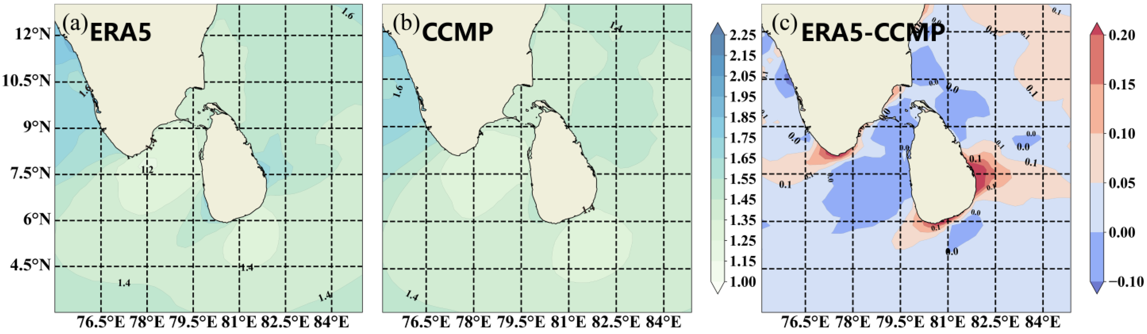
3.6. Wind Energy Stability

Assessing and developing wind energy requires considering the stability of WERs. As emphasized by Wang [31], both data dispersion and the stability of wind energy density are crucial factors in evaluating and selecting wind energy projects. Wind energy stability is commonly assessed using the Coefficient of Variation ($C_v$), a statistical metric quantifying variability relative to the dataset mean. It is particularly valuable for assessing WS consistency, which is essential for reliable wind power facility operation. The $C_v$ is given by [32]:

$$C_v=\frac{S}{\overline{x}}$$

(14)

$$S=\sqrt{\frac{{\sum }_{i=1}^n{x}_i^2-\left({\sum }_{i=1}^n{x}_i^2\right)/n}{n-1}}$$

(15)

$C_v$ represents the coefficient of variation, $\overline{x}$ denotes the mean value of WPD, while $x_i$ represents individual observations of WPD. A lower $C_v$ suggests a more stable and predictable wind resource, which is favorable for the feasibility and efficiency of wind energy projects. Being a dimensionless number, the $C_v$ allows for comparisons across different data sets, facilitating a relative assessment of wind resource stability irrespective of unit differences.

3.7. Weibull Distribution Function

The Weibull Distribution Function comprises statistical values employed to characterize WS data distribution. Due to its capability to fit diverse WS distributions effectively, it is extensively employed in modeling WS and environmental data probability distributions. This study employs the two-parameter Weibull distribution to analyze WS data characteristics across 16 directions, following the Weibull distribution [33,34]:

$$f\left(v,k,\lambda \right)=\frac{k}{\lambda }{\left(\frac{v}{\lambda }\right)}^{k-1}{\mathrm{e}}^{-{\left(\frac{v}{\lambda }\right)}^k }$$

(16)

here, $f$ represents the probability density function (PDF) of the Weibull distribution; $v$ denotes the observed WS; $k$ stands for the shape parameter; and $\lambda$ represents the scale parameter. In each direction, we employ maximum likelihood estimation to determine both the shape parameter $k$ and scale parameter $\lambda$ of the Weibull distribution.

4. Discussion of Results

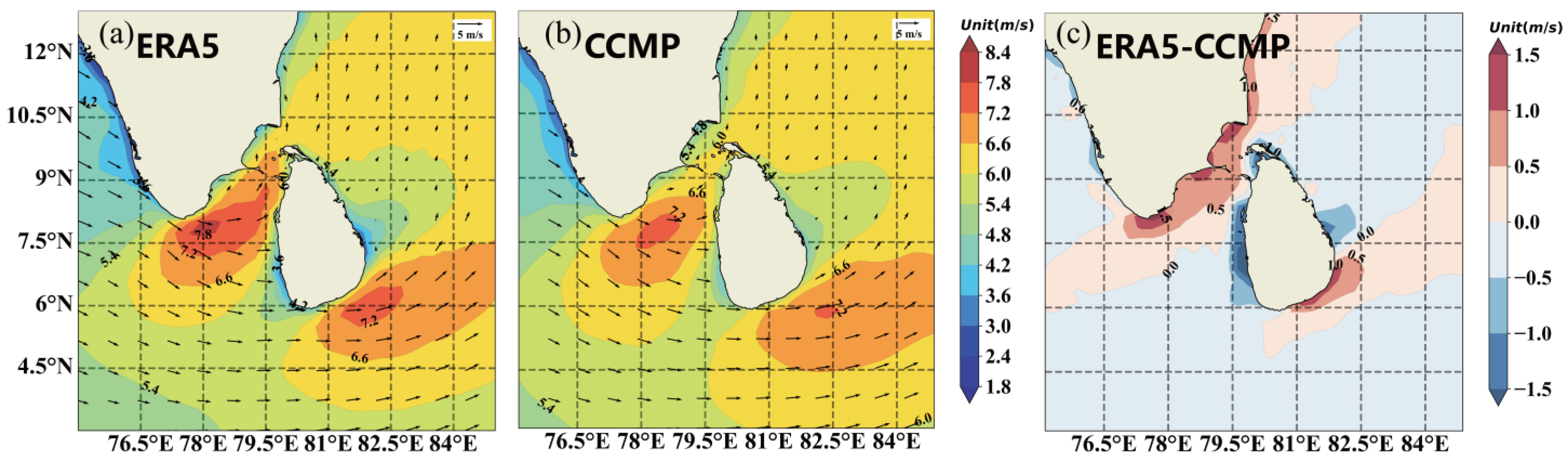
4.1. Wind Field Characterization

This study presents a thorough analysis of wind field characteristics over the Sri Lankan Sea. Based on the ocean flux tower data from 10 April 2017 to 3 September 2018, combined with CCMP, ERA5 analyzed the seasonal changes in WS, which is shown in Figure 2. We employ the moving average method to compute the daily moving average for each dataset and represent it graphically as a line. The fitting of CCMP and ERA5 data to measured data from June to August is relatively accurate, potentially attributed to the stable and robust monsoon activity prevalent during this period, which might enhance the models’ capacity to simulate actual wind speeds effectively. However, both the CCMP and ERA5 datasets tend to overestimate wind speeds from December to February, indicating possible limitations in their ability to capture the intricacies of the northeast monsoon’s influence on the region’s wind field dynamics.

Table 2. The variance contribution rates of the first four modes of EOF.

MODES	Mode1	Mode2	Mode3	Mode4
CCMP	60.02%	14.77%	5.18%	3.24%
ERA5	58.60%	13.96%	4.77%	3.18%

presents the results of the Empirical Orthogonal Function (EOF) analysis conducted on 35 years of wind field data from CCMP and ERA5, highlighting the variance contribution percentages of the first four modes. The analysis of EOF demonstrates that for the CCMP dataset, the first mode Figure 3(a1) accounts for 60.02% of the variance, followed by the second mode Figure 3(b1) at 14.77%, the third mode Figure 3(c1) at 5.18%, and the fourth mode Figure 3(d1) at 3.24%, with a total cumulative variance contribution from these four modes reaching 83.21%. Similarly, the ERA5 dataset shows the first mode Figure 3(a2) contributing 58.60% to the variance, the second mode Figure 3(b2) at 13.96%, the third mode Figure 3(c2) at 4.77%, and the fourth mode Figure 3(d2) at 3.18%, leading to an identical cumulative variance contribution of 83.21% from the top four modes. This suggests that the primary four modes extracted from both datasets are significant and effectively capture the main characteristics of the studied data.

The spatial distribution of EOF is shown in Figure 3. The percentage of the first mode’s variance contribution for the two datasets is 60.02% and 58.60%, respectively. This reflects the main characteristics of WS variation in the sea off Sri Lanka. The negative value for the entire region indicates synchronized increases and decreases in WS in the sea off Sri Lanka, demonstrating spatial consistency in the change. The proportion of the second mode variance contribution is 14.77% and 13.96%, respectively, which also explains the spatial distribution characteristics of the sea area to some extent. Bounded by the line connecting the Indian Peninsula and Sri Lanka, it shows a southwest-northeast symmetric structure, with positive values in the northeast, negative values in the southwest, and an inverse correlation on both sides of the southwest-northeast. The percentage of variance contribution of the third mode is 5.18% and 4.77%, respectively, showing a northwest-southeast symmetric structure, with an overall value close to 0, which indicates that there is little change in the region. However, positive values can be seen in the ERA5 data for the western side of peninsular India and negative values for CCMP. The fourth mode variance contribution percentage is 3.24% and 3.18%, respectively, and a clear negative zone can be seen on the western side of peninsular India, with the rest of the region showing less variation.

The time series reflects a clear seasonal variation. A positive time-varying coefficient of the first mode Figure 3(a3) corresponds to a decrease in wind speeds across the entire vicinity of Sri Lanka, while a negative coefficient indicates an increase in wind speeds in the same area. Similarly, a positive time-varying coefficient of the second mode Figure 3(b3) results in increased wind speed values north of the Indo-Sri Lanka link and decreased wind speeds south of it. Conversely, negative coefficient variations yield opposite effects. In the third mode Figure 3(c3), positive time coefficient variations lead to decreased wind speeds in the Lakshadweep Sea and increased speeds in the southeastern region, with opposite changes for negative time coefficient variations. Finally, in the fourth mode, Figure 3(d3), positive time coefficient variations cause a decrease in wind speed on the western side of the Indian Peninsula.

It can be concluded that the wind field in Sri Lanka has significant seasonal and regional characteristics, and the time series mainly shows seasonal oscillatory variations, and the amplitude has not changed much during the 35 years in first mode, indicating that the wind field activity in the sea off Sri Lanka has changed very little in these 35 years.

4.2. Analysis of Wind Speed

Accurate analysis of the spatial and temporal variability of the wind field off Sri Lanka is a prerequisite for wind resource development. By utilizing two different data sources, CCMP and ERA5, we are able to analyze the dynamics of the wind field from multiple perspectives, reducing the dependence on a single data source and improving the reliability and comprehensiveness of the analysis. By comparing and plotting the difference, this paper effectively demonstrates the differences in WS distribution between the two data sources, especially the specific results regarding the mean WS in different climatic states and seasons.

The analysis in Figure 4 indicates that the annual average WS exceeds 5.4 m/s in most areas of the sea off Sri Lanka, suggesting good potential for wind energy development. Particularly noteworthy is the region between the northwestern part of Sri Lanka and the coast of the Indian Peninsula, as well as the southeastern sea, where the annual average WS can reach 6.6 m/s, making it a high-value area for WERs. Conversely, the southern coast of Sri Lanka experiences lower WS, which represents a potential low-value area.

The Indian Ocean, due to its unique geographical location, is significantly influenced by monsoon winds throughout the year, resulting in large variations in WS in different seasons. In order to understand the impact of such seasonal variations on the WERs in the sea off Sri Lanka, the present study plots the seasonal annual mean WS and analyzes the variation of WS in the four seasons of MAM (March, April, and May), JJA (June, July, and August), SON (September, October, and November), and DJF (December, January and February of the following year) [35].

The average WS in the region is characterized by a clear seasonal distribution, which is shown in Figure 5. During the JJA season, under the influence of the strong and regular southwestern monsoon, the average WS is the highest and can reach more than 7.2 m/s in most areas, indicating that this is the season with the most abundant WERs in the whole year. In contrast, the DJF season is influenced by the northeast monsoon, with the WS above 5.4 m/s in some parts of the sea off Sri Lanka, while the WS is the smallest during the MAM. This shows that the JJA and DJF seasons are influenced by northeast and southwest winds, respectively, while MAM and SON are transitional seasons.

Figure 6 shows a wind rose diagram of average WS distributions from 1988 to 2022 for two datasets (ERA5 and CCMP). Wind rose diagrams are statistical charts used to represent WS and direction data, commonly utilized in meteorology and oceanography research. In these two diagrams, each sector represents a specific wind direction, while different colors indicate different WS ranges, and the numbers on the concentric circles represent WS frequencies.

In the ERA5 data, Figure 6a illustrates the annual average wind direction and wind frequency distribution. It is evident that the primary wind direction in the study area is WSW and neighboring directions, followed by the NE and several adjacent directions, forming a cluster distribution. The maximum WS is observed in WSW, constituting approximately 14.0%, followed by SW and W, with wind frequencies of around 11.3% and 11.0%, respectively. Conversely, in Figure 6b, CCMP displays similar wind directions, yet NE and surrounding directions represent a larger proportion compared to ERA5.

While both datasets showcase similar predominant wind directions, there exist disparities in the specific percentage values. These variations could arise from discrepancies in data processing methods and measurement techniques.

From the results depicted in Figure 7, it is evident that there is a noticeable seasonality in wind direction changes. Throughout the MAM, JJA, and SOD periods, WSW dominated as the primary wind direction, whereas during the DJF period, it shifted to the NE. In the ERA5 data (Figure 7a–d), during MAM, the predominant wind direction is WSW, comprising 12.1% of the wind frequency, followed by SW, with distribution across other directions except N. Similarly, during JJA, WSW represents the largest proportion of wind direction, accounting for 26.8%. The overall WS is relatively high, and the direction is focused. In contrast, during SOD, there is a small cluster of northeasterly winds, and the proportion of the primary WSW wind direction decreases. DJF and NE emerge as the predominant wind directions, accounting for 29.5%, with wind speeds reaching up to 10.2 m/s, followed by NNE and ENE.

In the CCMP data (Figure 7e–h), the distribution mirrors that of ERA5. However, based on the percentage distribution, it is noticeable that the CCMP data exhibit greater concentration, with wind frequencies depicted in the figure being consistently higher than those in ERA5.

In order to further determine the WS distribution in each direction, we used the Weibull function to further study the probability density function (PDF) distribution in each direction.

The CCMP data results are depicted in Figure 8, revealing notable differences in probability density functions (PDF) across various orientations. Figure 8f–h illustrate that the WS distribution is more concentrated in the NNE, NW, and WNN directions, ranging from 0 to 10 m/s. However, the wind speeds are relatively low, with a frequency value of approximately 3 m/s, and wind speed frequencies exceeding 20%. Conversely, in Figure 8b,c,j,k,i,m,n, corresponding to the ENE, NE, WSW, SW, SSW, S, and SSE directions, respectively, peak wind speeds reach around 7.5 m/s, indicating relatively higher wind speeds. While WSW emerges as the dominant WS direction in Figure 6a, the Weibull parameter method shows a less concentrated wind speed distribution, primarily clustered between 5 and 7.5 m/s.

Figure 9 presents the outcomes of the Weibull function applied to ERA5 data. The distribution appears akin to that of the CCMP data. However, in Figure 9h, a distinct difference is observed in the WNW direction. The ERA5 wind speed data distribution exhibits greater concentration, with a wind speed of approximately 3.5 m/s, and the wind speed frequency reaching 25%.

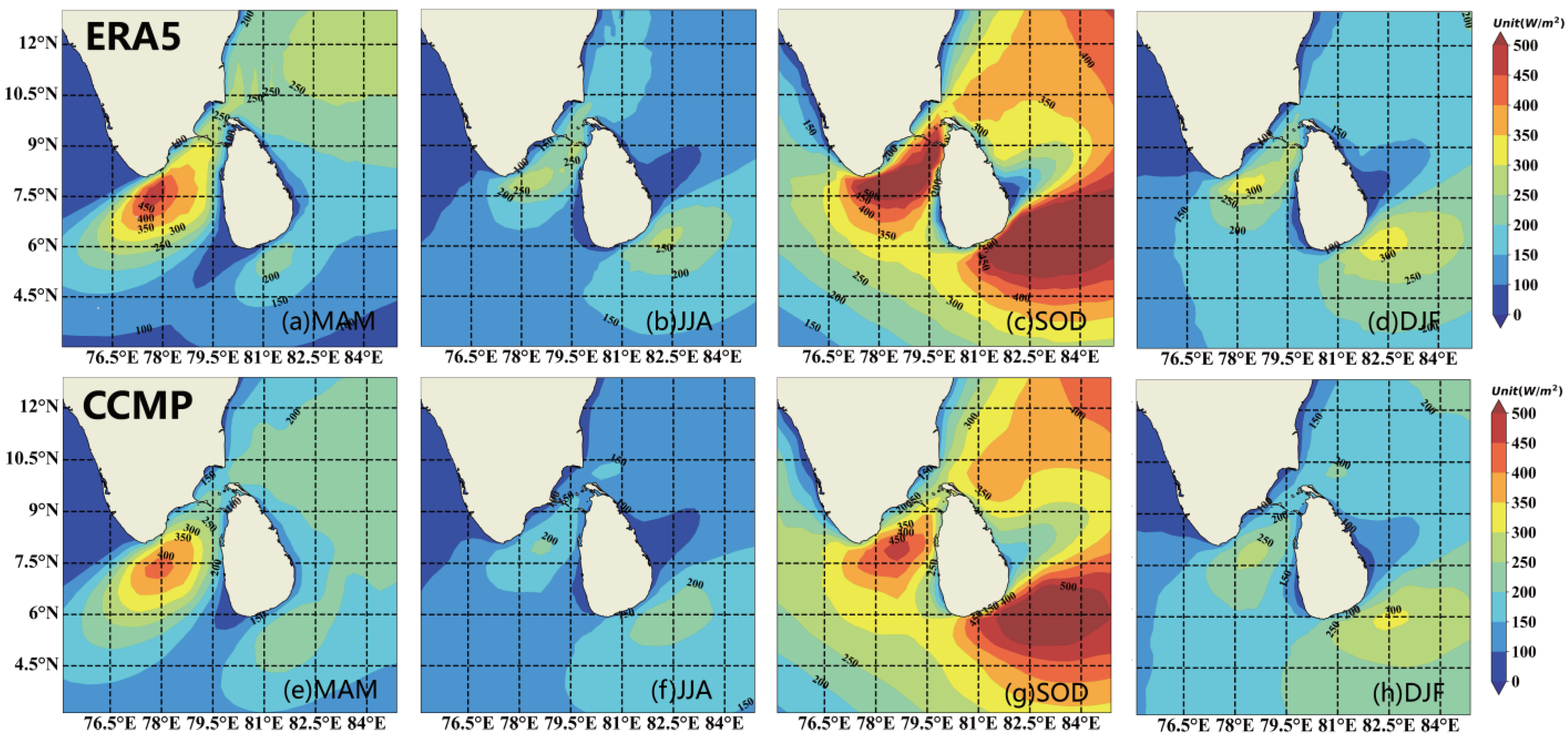
4.3. Analysis of Wind Energy Potential

Through the preceding analysis of WS, we have gained a comprehensive understanding of its characteristics. Building upon this foundation, we proceeded to further analyze the wind energy density potential of the wind field. WPD directly reflects the analysis of wind energy abundance, typically considered available for densities exceeding 100 W/m² and abundant for densities exceeding 200 W/m². Figure 10 illustrates that the majority of annual average WPD in this sea area exceeds 150 W/m², with about half of the area reaching 200 W/m², indicating a region abundant in WERs.

The seasonal WPD analysis presented in Figure 11 reveals a clear seasonal characterization of the wind resource in the sea off Sri Lanka. During the period from June to August, the WPD increases significantly and reaches more than 200 W/m² in most areas, especially in most parts of the Sri Lankan vicinity, where the WPD even reaches 250 W/m² during the season, which signifies that this is a very rich area in terms of WERs. In particular, the area between the northwestern part of the Sri Lankan landmass and the coast of the Indian Peninsula, as well as the southeastern part of the sea, can reach wind power densities of more than 400 W/m², which further highlights the potential of these high-value zones in terms of wind resource development. In contrast, WPD is the next highest from December to February, while the period from March to May is relatively poor. In general, wind conditions from June to August are more favorable for wind resource development.

The stability of WERs is particularly important for wind energy development, and the coefficient of variation (CV) is a key indicator of this stability, with smaller values indicating more stable WERs. In this study, the distribution of the CV in the sea area off Sri Lanka is analyzed in detail using both CCMP and ERA5 data and is presented in a difference plot (Figure 12). The results of the analysis show that the WERs in the sea off Sri Lanka are overall stable and the two data show a small difference in the CV, which is within 0.2, implying the reliability of wind energy in the area. The distribution of the coefficient of variation in different seasons shows a clear seasonal pattern, especially during the period from June to August, when the WER exhibits higher stability (Figure 13).

In order to assess the effectiveness of WS, the effective wind speed occurrence (EWSO) was defined as the proportion of the total number of time steps with WS between 3 and 25 m/s. By plotting the EWSO distribution (Figure 14), it can be observed that the EWSO can reach 80% in most of the Sri Lankan sea area, especially in the area between the Indian Peninsula and Sri Lanka, where the EWSO can even reach 90%. This result indicates that the WS in the region is within the effective range for wind power generation most of the time, and the difference in the EWSO distribution between the two types of data in the ocean area is small.

According to the previous section, we already know that the WS, mean WPD, coefficient of variation (CV), and effective wind occurrence off Sri Lanka have significant seasonal characteristics, and in order to further explore this characteristic, this paper further analyzes the monthly variations of these four variables. Observing Figure 15a, which shows the monthly variation of the mean WS for 35 years, it is found that the mean WS peaks in June–August, followed by December–January, and is lower in March–April and October–November, showing a “W” trend. This is consistent with the previous results on seasonal variations. Figure 15b shows similar results for the 35-year monthly variation of mean WPD and mean WS, both of which peak in June and are lowest in March. Figure 15c shows the monthly variation of the CV of the 35-year mean WPD, and it can be seen that the CV is low from June to September, and the CV is relatively high in March, April, and November. Figure 15d demonstrates the monthly variation of EWSO for 35 years, reflecting that the EWSO is above 60% throughout the year and reaches above 90% in all months except March, April, October, and November, with a good availability of WS.

4.4. Total Wind Energy Reserves and Technically Exploitable Capacity

Table 3. Wind energy total reserves and technically exploitable capacity.

	Total Wind Energy Capacity	Technically Exploitable Capacity
CCMP	2.00 GW	1.58 GW
ERA5	2.07 GW	1.63 GW

shows wind energy total reserves and technically exploitable capacity in our study area. The total wind resource estimated from the CCMP data is 2.00 GW, while its technically exploitable capacity is estimated at 1.58 GW. Conversely, calculations using ERA5 data yield a slightly higher total wind resource reserve of 2.07 GW and a technically exploitable amount of 1.63 GW. These results suggest that the differences between the total wind energy reserves and the technically exploitable capacities, obtained from the climate state studies using different data sources, are not significant.

This close agreement further confirms the consistency and reliability of both data sources in assessing WERs off the coast of Sri Lanka. The calculations of total reserves and technically exploitable capacities provide crucial reference data for the planning and development of wind power projects in the region. Notably, the estimation of technically exploitable capacity is critical for determining the economics and feasibility of wind energy utilization and serves as a key basis for future wind farm siting and design.

5. Conclusions

This study offers a comprehensive analysis of wind field characteristics, the potential of wind energy, its seasonal variations, and both the total and technically exploitable WERs in the sea off Sri Lanka. It leverages data from two sources, CCMP and ERA5, alongside actual station data. The two data analysis results exhibit minimal disparity. Key findings and conclusions include:

Wind Field Characterization: The study reveals a distinct seasonal distribution of wind speeds off Sri Lanka, particularly noting an increase from June to August due to the southwest monsoon. This period is identified as having the richest WERs. In the waters near Sri Lanka, two predominant wind directions are observed: WSW and NE. However, significant differences exist in wind speed across various directions, such as ENE, NE, WSW, SW, SSW, S, and SSE. These directions experience higher wind speeds. Conversely, the WS distribution is more concentrated in the NNW, NW, and WNN directions, with lower wind speeds.

Wind Energy Potential and Seasonal Variations: Seasonal analysis of average WS and wind power densities confirms the abundance of WERs off Sri Lanka, especially from June to August. WPD in this area can exceed 200 W/m², with some regions reaching above 400 W/m², showcasing a high potential for wind energy development. Meanwhile, based on the CV results, the overall wind energy in the study area appears stable.

Total and Technically Exploitable Wind Energy Reserves: Based on CCMP and ERA5 data, the total WERs are estimated at 2.00 GW and 2.07 GW, respectively, with a technically exploitable capacity of 1.58 GW and 1.63 GW. These figures indicate significant WERs off Sri Lanka, with a promising technically exploitable capacity.

Consistency and Reliability of Dlkjata: The study validates the CCMP and ERA5 datasets against measurements from Sri Lankan flux towers, confirming their reliability for assessing WERs off Sri Lanka. The negligible differences in total wind energy reserves and technically exploitable amounts between the datasets underscore their consistency and reliability, providing a robust foundation for future assessments.

In conclusion, this study furnishes essential data and a scientific basis for developing WERs off Sri Lanka. By elucidating the distribution of WS and WPD across seasons, and quantifying the total and technically exploitable WERs, it sets a direction for future wind power project planning and construction. These insights are vitally important for advancing sustainable energy development in Sri Lanka and its vicinity, and offer valuable lessons for other regions with similar geographic and climatic conditions.

References

1. Buonocore, J.J.; Luckow, P.; Fisher, J.; Kempton, W.; Levy, J.I. Health and Climate Benefits of Offshore Wind Facilities in the Mid-Atlantic United States. Environ. Res. Lett. 2016, 11, 074019. [Google Scholar] [CrossRef]
2. Vázquez Hernández, C.; Serrano González, J.; Fernández-Blanco, R. New Method to Assess the Long-Term Role of Wind Energy Generation in Reduction of CO2 Emissions—Case Study of the European Union. J. Clean. Prod. 2019, 207, 1099–1111. [Google Scholar] [CrossRef]
3. Veers, P.; Dykes, K.; Lantz, E.; Barth, S.; Bottasso, C.L.; Carlson, O.; Clifton, A.; Green, J.; Green, P.; Holttinen, H.; et al. Grand Challenges in the Science of Wind Energy. Science 2019, 366, eaau2027. [Google Scholar] [CrossRef] [PubMed]
4. Weisser, D. A Wind Energy Analysis of Grenada: An Estimation Using the ‘Weibull’ Density Function. Renew. Energy 2003, 28, 1803–1812. [Google Scholar] [CrossRef]
5. Pimenta, F.; Kempton, W.; Garvine, R. Combining Meteorological Stations and Satellite Data to Evaluate the Offshore Wind Power Resource of Southeastern Brazil. Renew. Energy 2008, 33, 2375–2387. [Google Scholar] [CrossRef]
6. Mahmuddin, F.; Idrus, M.; Hamzah. Analysis of Ocean Wind Energy Density around Sulawesi and Maluku Islands with Scatterometer Data. Energy Procedia 2015, 65, 107–115. [Google Scholar] [CrossRef]
7. Bruunchristiansen, M.; Koch, W.; Horstmann, J.; Bayhasager, C.; Nielsen, M. Wind Resource Assessment from C-Band SAR. Remote Sens. Environ. 2006, 105, 68–81. [Google Scholar] [CrossRef]
8. Salvação, N.; Guedes Soares, C. Wind Resource Assessment Offshore the Atlantic Iberian Coast with the WRF Model. Energy 2018, 145, 276–287. [Google Scholar] [CrossRef]
9. Pryor, S.C.; Barthelmie, R.J. Assessing Climate Change Impacts on the Near-Term Stability of the Wind Energy Resource over the United States. Proc. Natl. Acad. Sci. USA 2011, 108, 8167–8171. [Google Scholar] [CrossRef] [PubMed]
10. Dong, C.; Huang, G.; Cheng, G. Offshore Wind Can Power Canada. Energy 2021, 236, 121422. [Google Scholar] [CrossRef]
11. Contestabile, P.; Lauro, E.D.; Galli, P.; Corselli, C.; Vicinanza, D. Offshore Wind and Wave Energy Assessment around Malè and Magoodhoo Island (Maldives). Sustainability 2017, 9, 613. [Google Scholar] [CrossRef]
12. Putro, W.S.; Prahmana, R.A.; Yudistira, H.T.; Darmawan, M.Y.; Triyono, D.; Birastri, W. Estimation Wind Energy Potential Using Artificial Neural Network Model in West Lampung Area. IOP Conf. Ser. Earth Environ. Sci. 2019, 258, 012006. [Google Scholar] [CrossRef]
13. Archer, C.L.; Jacobson, M.Z. Evaluation of Global Wind Power. J. Geophys. Res. 2005, 110, 2004JD005462. [Google Scholar] [CrossRef]
14. Capps, S.B.; Zender, C.S. Estimated Global Ocean Wind Power Potential from QuikSCAT Observations, Accounting for Turbine Characteristics and Siting. J. Geophys. Res. 2010, 115, 2009JD012679. [Google Scholar] [CrossRef]
15. Zheng, C.W.; Pan, J. Assessment of the Global Ocean Wind Energy Resource. Renew. Sustain. Energy Rev. 2014, 33, 382–391. [Google Scholar] [CrossRef]
16. Zheng, C.; Li, X.; Luo, X.; Chen, X.; Qian, Y.; Zhang, Z.; Gao, Z.; Du, Z.; Gao, Y.; Chen, Y. Projection of Future Global Offshore Wind Energy Resources Using CMIP Data. Atmos.-Ocean 2019, 57, 134–148. [Google Scholar] [CrossRef]
17. Zheng, C.; Yi, C.; Shen, C.; Yu, D.; Wang, X.; Wang, Y.; Zhang, W.; Wei, Y.; Chen, Y.; Li, W.; et al. A Positive Climatic Trend in the Global Offshore Wind Power. Front. Energy Res. 2022, 10, 867642. [Google Scholar] [CrossRef]
18. Yang, S.; Duan, S.; Fan, L.; Zheng, C.; Li, X.; Li, H.; Xu, J.; Wang, Q.; Feng, M. 10-Year Wind and Wave Energy Assessment in the North Indian Ocean. Energies 2019, 12, 3835. [Google Scholar] [CrossRef]
19. Kumar, V.; Asok, A.; George, J.; Amrutha, M. Regional Study of Changes in Wind Power in the Indian Shelf Seas over the Last 40 Years. Energies 2020, 13, 2295. [Google Scholar] [CrossRef]
20. Patel, R.P.; Nagababu, G.; Kachhwaha, S.S.; Arun Kumar, S.V.V.; M, S. Combined Wind and Wave Resource Assessment and Energy Extraction along the Indian Coast. Renew. Energy 2022, 195, 931–945. [Google Scholar] [CrossRef]
21. Patel, R.P.; Nagababu, G.; Kachhwaha, S.S.; Surisetty, V.V.A.K. A Revised Offshore Wind Resource Assessment and Site Selection along the Indian Coast Using ERA5 Near-Hub-Height Wind Products. Ocean. Eng. 2022, 254, 111341. [Google Scholar] [CrossRef]
22. Chacko, N. Exploring the Offshore Wind Resource Potential of India Based on Remotely Sensed Wind Field Data. J. Indian Soc. Remote Sens. 2022, 50, 1689–1700. [Google Scholar] [CrossRef]
23. Chandrasena, R.P.S.; Vikkitharan, G.; Arulampalam, A.; Ekanayake, J.B. Constraints for the Development of Wind Power Generation in Sri Lanka. In Proceedings of the First International Conference on Industrial and Information Systems, Tirtayasa, Indonesia, 8–11 August 2006; pp. 221–226. [Google Scholar]
24. Stow, C.A.; Roessler, C.; Borsuk, M.E.; Bowen, J.D.; Reckhow, K.H. Comparison of Estuarine Water Quality Models for Total Maximum Daily Load Development in Neuse River Estuary. J. Water Resour. Plann. Manag. 2003, 129, 307–314. [Google Scholar] [CrossRef]
25. Leggett, R.W.; Williams, L.R. A Reliability Index for Models. Ecol. Model. 1981, 13, 303–312. [Google Scholar] [CrossRef]
26. Nan, X.; Li, Q.; Qiu, D.; Zhao, Y.; Guo, X. Short-Term Wind Speed Syntheses Correcting Forecasting Model and Its Application. Int. J. Electr. Power Energy Syst. 2013, 49, 264–268. [Google Scholar] [CrossRef]
27. Pearson, K. LIII. On Lines and Planes of Closest Fit to Systems of Points in Space. Lond. Edinb. Dublin Philos. Mag. J. Sci. 1901, 2, 559–572. [Google Scholar] [CrossRef]
28. Zheng, C.; Zhuang, H.; Li, X.; Li, X. Wind Energy and Wave Energy Resources Assessment in the East China Sea and South China Sea. Sci. China Technol. Sci. 2012, 55, 163–173. [Google Scholar] [CrossRef]
29. Ding, J.; Wu, G.; Chen, J.; Jiang, B. Study on the Assessment of Marine Wind Energy Resources in the South China Sea Based on CCMP Reanalysis (in Chinese) Wind Field Data. J. Ocean. Technol. 2022, 41, 83–90. [Google Scholar]
30. National Energy Administration. Notice of the National Development and Reform Commission on Issuing the “Technical Regulations for National Wind Energy Resource Assessment” [EB/OL]. (2004-05-14). Available online: http://www.nea.gov.cn/2012-01/04/c_131260326.htm (accessed on 4 January 2012).
31. Wang, C.K.; Lu, W. Analysis Methods and Reserves Evaluation of Ocean Energy Resources; Ocean Press: Beijing, China, 2009; pp. 272–275. (In Chinese) [Google Scholar]
32. Zheng, C.; Song, H.; Liang, F.; Jin, Y.; Wang, D.; Tian, Y. 21st Century Maritime Silk Road: Wind Energy Resource Evaluation; Springer Oceanography; Springer: Singapore, 2021; ISBN 9789811641107. [Google Scholar]
33. Wais, P. A Review of Weibull Functions in Wind Sector. Renew. Sustain. Energy Rev. 2017, 70, 1099–1107. [Google Scholar] [CrossRef]
34. Aziz, A.; Tsuanyo, D.; Nsouandele, J.; Mamate, I.; Mouangue, R.; Elé Abiama, P. Influence of Weibull Parameters on the Estimation of Wind Energy Potential. Sustain. Energy Res. 2023, 10, 5. [Google Scholar] [CrossRef]
35. Elliott, D.; Schwartz, M.; Scott, G.; Haymes, S.; Heimiller, D.; George, R. Wind Energy Resource Atlas of Sri Lanka and the Maldives; NREL/TP-500-34518; National Renewable Energy Laboratory: Golden, CO, USA, 2003; p. 15004471. [Google Scholar]
Figure 1. Observation Site Location for Data Validation (Red Point) and Study Area.
Jmse 12 00876 g001
Figure 2. Mean Wind Speed Comparison: gray dot: Marine Flux Tower data; blue line: the daily moving average of Marine Flux Tower data; orange line: the daily moving average of ERA5 data; green line: the daily moving average of CCMP data.
Jmse 12 00876 g002
Figure 3. The EOF Distribution from 1988 to 2022: (a1d1): the first four modal spatial distributions of CCMP; (a2d2): the first four modal spatial distributions of ERA5; (a3d3): the monthly averaged time series plots of ERA5 and CCMP data, the red line represents CCMP data, and the black line represents ERA5 data.
Jmse 12 00876 g003
Figure 4. Spatial distribution of annual mean wind speed and direction during 1988–2022, (a) ERA5, (b) CCMP, and (c) The difference between ERA5 data and CCMP data. ( V d i f f e r e n c e = V E R A 5 V C C M P ).
Jmse 12 00876 g004
Figure 5. Spatial distribution of seasonal mean wind speed and direction during 1988−2022. MAM is March to May, JJA is June to August, SOD is September to November, DJF is December to February of the following year. (ad) are ERA5 data. (eh) are CCMP data.
Jmse 12 00876 g005
Figure 6. Wind rose diagram of wind speed distribution from 1988 to 2022. (a) is ERA5 data, and (b) is CCMP data.
Jmse 12 00876 g006
Figure 7. Wind rose diagram of seasonal distribution of wind speed during 1988−2022. (a) MAM, (b) JJA, (c) SOD, and (d) DJF are ERA5 data. (e) MAM, (f) JJA, (g) SOD, and (h) DJF are CCMP data.
Jmse 12 00876 g007
Figure 8. Weibull probability distribution in all directions from 1988 to 2022. (a) E: East, (b) ENE: East-Northeast, (c) NE: Northeast, (d) NNE: North-Northeast, (e) N: North, (f) NNW: North-Northwest, (g) NW: Northwest, (h) WNW: West-Northwest, (i) W: West, (j) WSW: West-Southwest, (k) SW: Southwest, (l) SSW: South-Southwest, (m) S: South, (n) SSE: South-Southeast, (o) SE: Southeast, (p) ESE: East-Southeast. x-axis: wind speed; y-axis: probability density function (PDF). Red line: Weibull distribution of wind speed probability; λ: scale parameter; k: shape parameter.
Jmse 12 00876 g008
Figure 9. Weibull probability distribution in all directions from 1988 to 2022. (a) E: East, (b) ENE, (c) NE, (d) NNE, (e) N, (f) NNW, (g) NW, (h) WNW, (i) W, (j) WSW, (k) SW, (l) SSW, (m) S: South, (n) SSE, (o) SE, (p) ESE. x-axis: wind speed; y-axis: probability density function (PDF). Red line: Weibull distribution of wind speed probability; λ: scale parameter; k: shape parameter.
Jmse 12 00876 g009
Figure 10. Spatial distribution of annual mean WPD (wind power density) during 1988−2022, (a) ERA5, (b) CCMP, and (c) The difference between ERA5 data and CCMP data. ( W P D d i f f e r e n c e = W P D E R A 5 W P D C C M P ).
Jmse 12 00876 g010
Figure 11. Spatial distribution of seasonal mean WPD (wind power density) during 1988−2022. (a) MAM, (b) JJA, (c) SOD, and (d) DJF are ERA5 data. (e) MAM, (f) JJA, (g) SOD, and (h) DJF are CCMP data.
Jmse 12 00876 g011
Figure 12. Spatial distribution of annual mean CV (coefficient of variation) during 1988−2022, (a) ERA5, (b) CCMP, and (c) The difference between ERA5 data and CCMP data. ( C V d i f f e r e n c e = C V E R A 5 C V C C M P ).
Jmse 12 00876 g012
Figure 13. Spatial distribution of seasonal CV (coefficient of variation) during 1988−2022. (a) MAM, (b) JJA, (c) SOD, and (d) DJF are ERA5 data. (e) MAM, (f) JJA, (g) SOD, and (h) DJF are CCMP data.
Jmse 12 00876 g013
Figure 14. Spatial distribution of EWSO (Effective Wind Speed Occurrence) during 1988−2022, (a) ERA5, (b) CCMP, and (c) The difference between ERA5 data and CCMP data. ( E W S O d i f f e r e n c e = E W S O E R A 5 E W S O C C M P ) Blue represents when the EWSO of ERA5 data is less than CCMP, while red represents the opposite.
Jmse 12 00876 g014
Figure 15. Monthly distribution of changes from 1988 to 2022: (a) Monthly variation of average WS; (b) Monthly variation of average WPD; (c) Monthly variation of coefficient of variation; (d) Monthly variation of EWSO. Blue represents ERA5 data, while red represents CCMP data.
Jmse 12 00876 g015