
Vertical Distribution of Rip Currents Generated by Intersecting Waves in a Sandbar–Groin Systems

Abstract
:1. Introduction
2. Experimental Set-Up
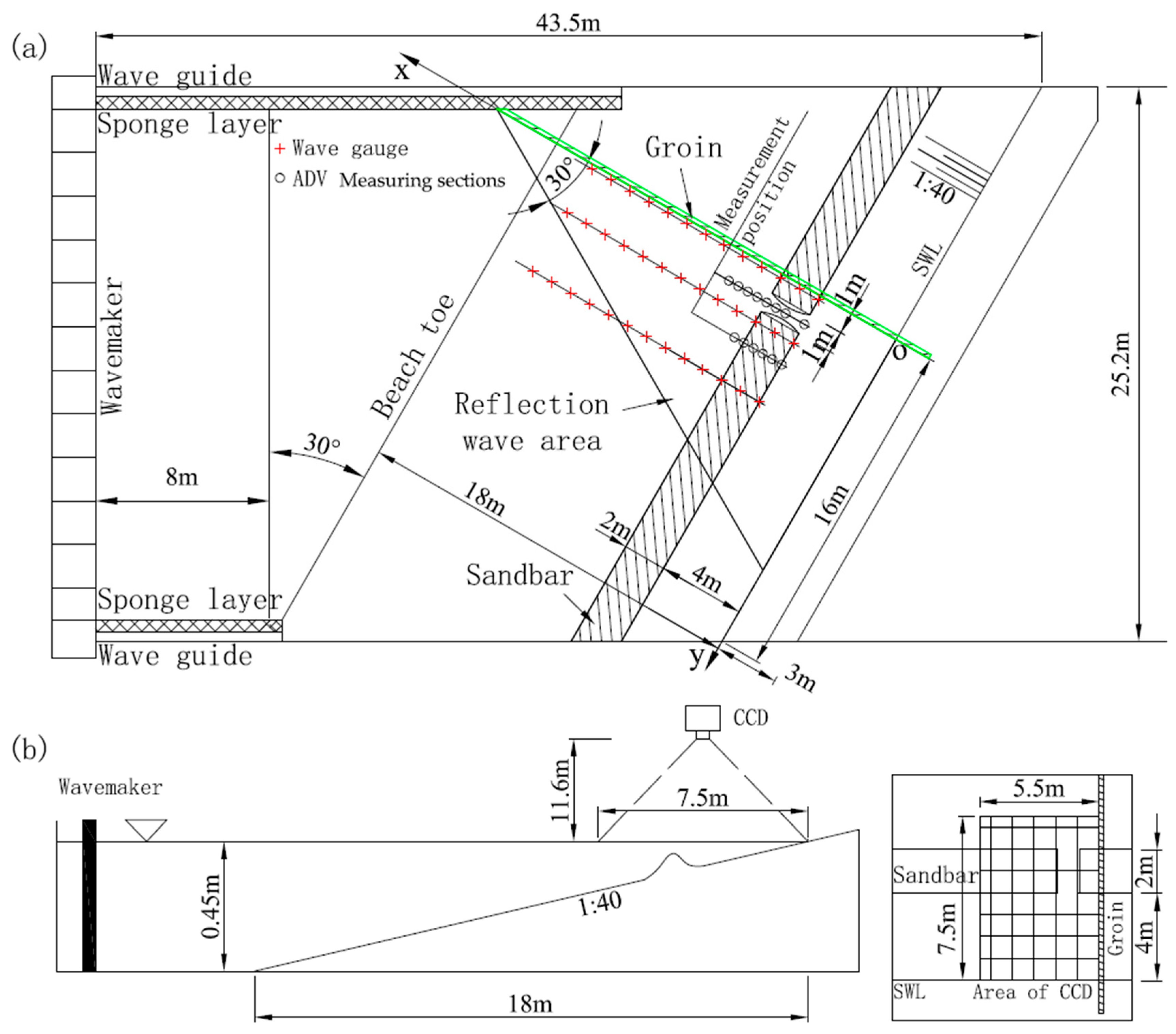
2.1. Experimental Lay-Out
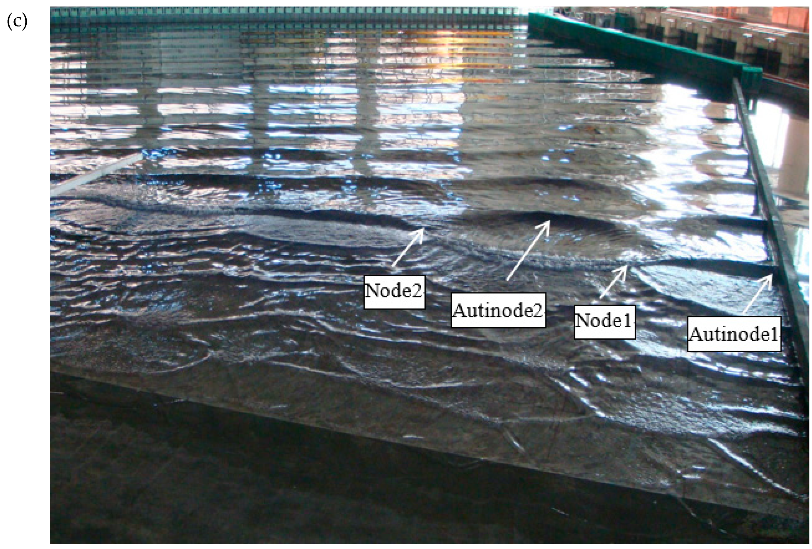
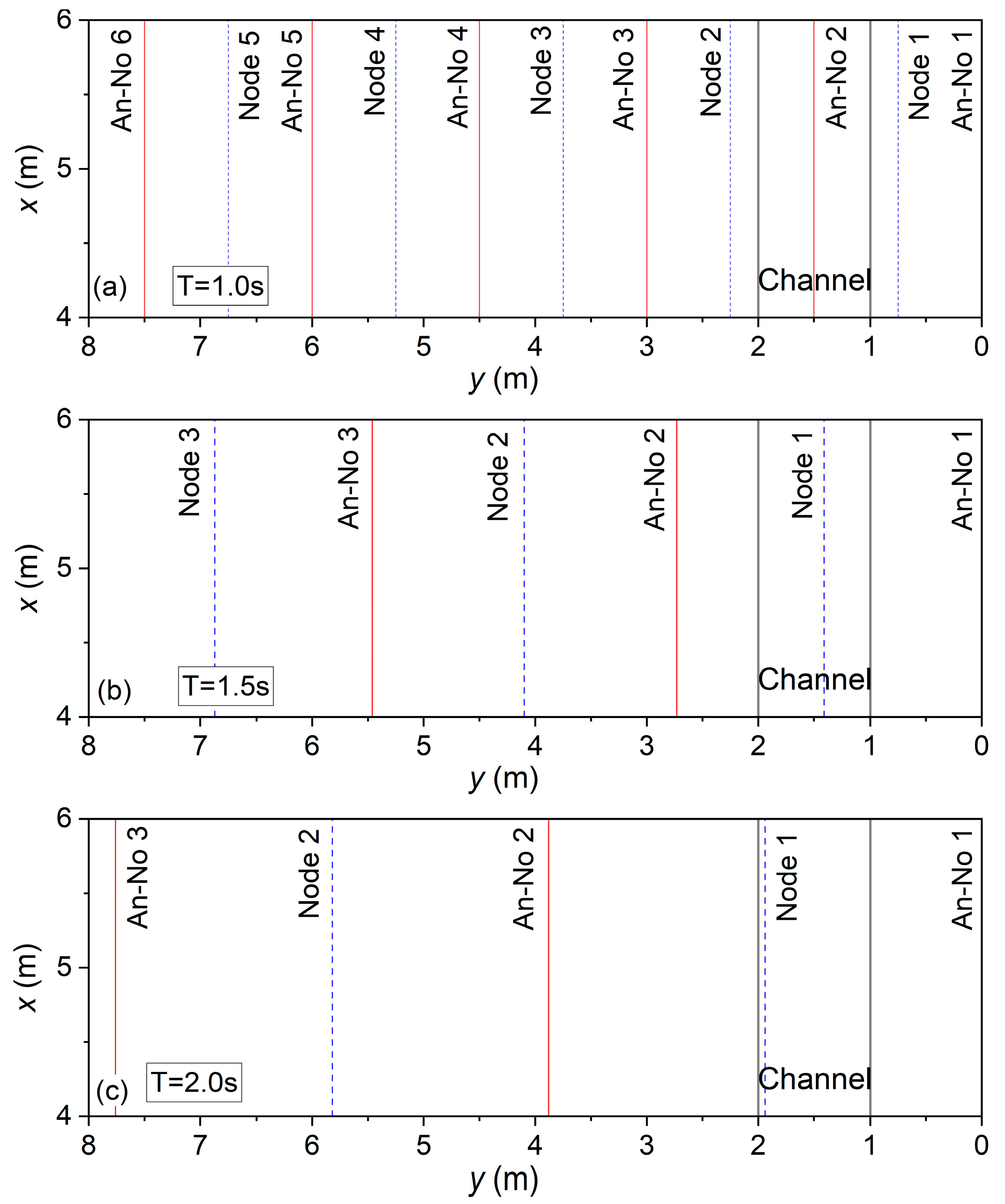
2.2. Wave Fields and Measurements
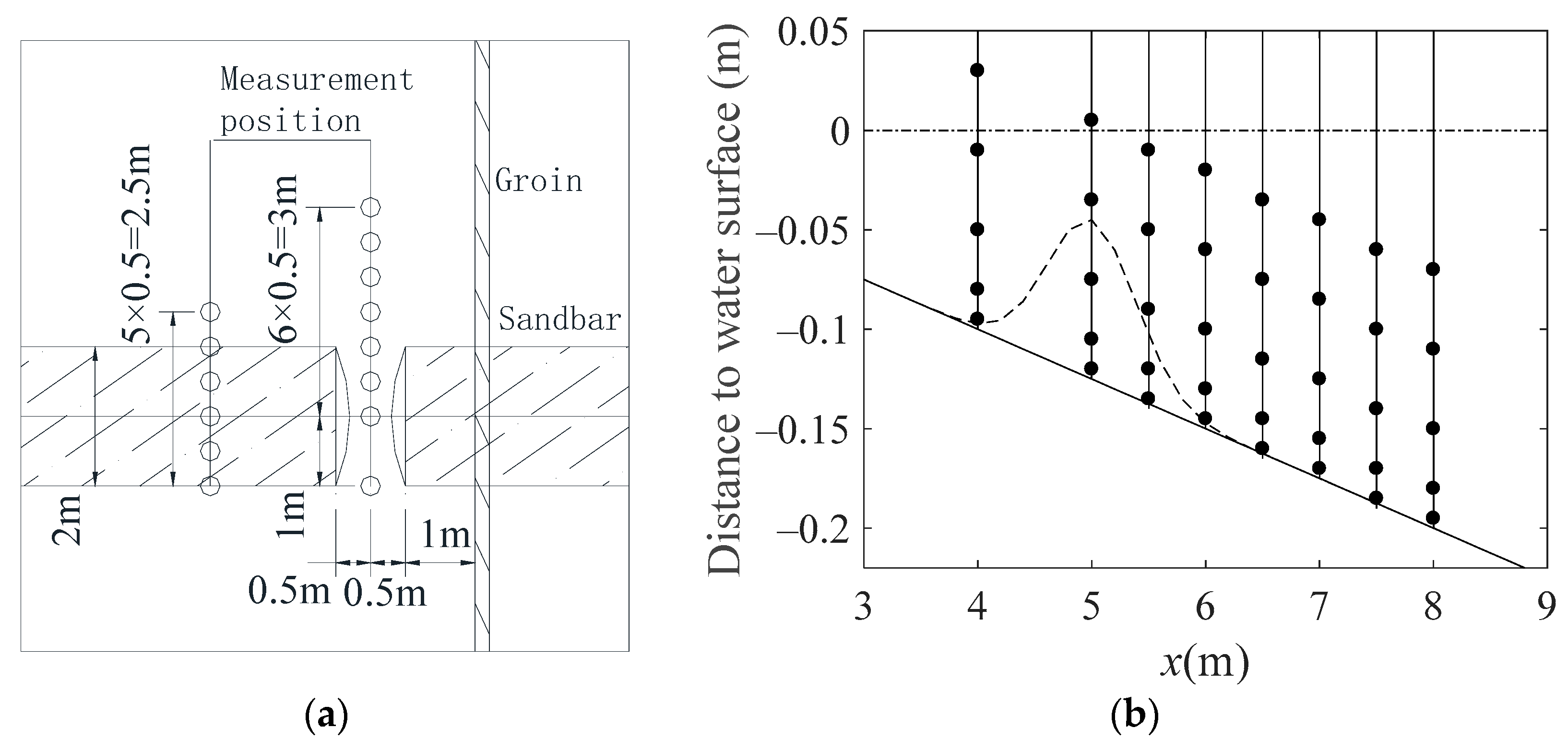
2.3. Measurement Methods of Vertical Distribution Measurements
3. Theoretical Analysis of Rip Current Characteristics
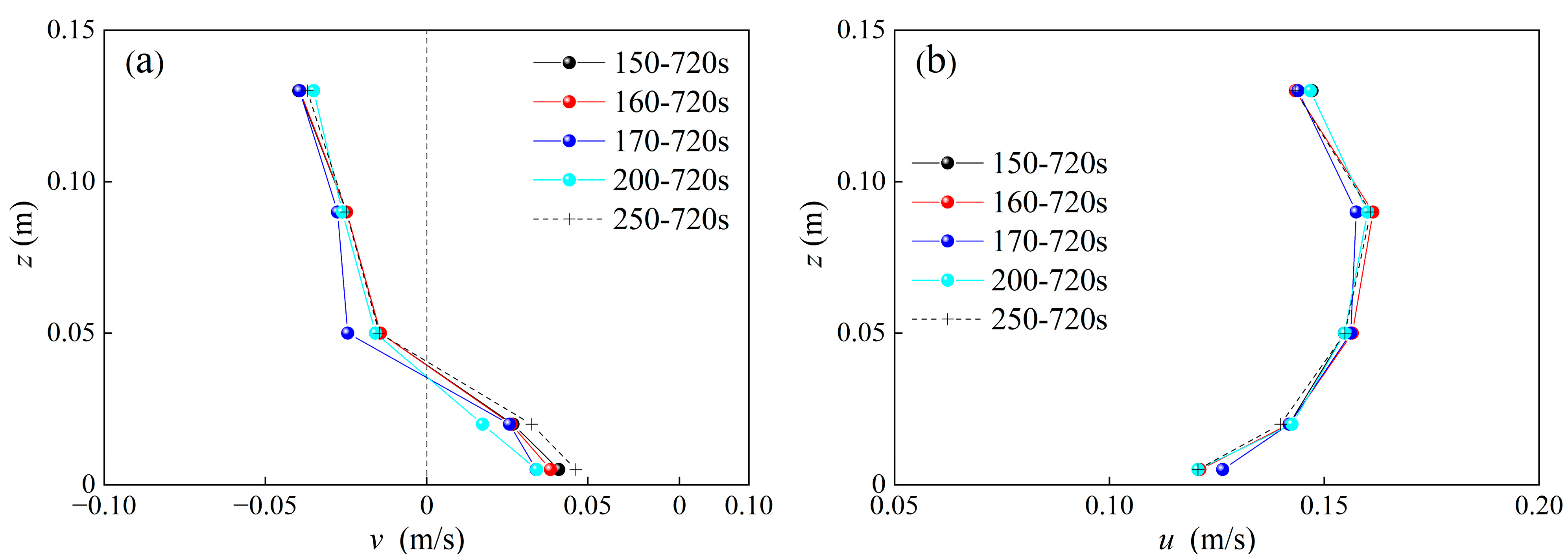
3.1. Time-Varying Characteristic of Rip Current
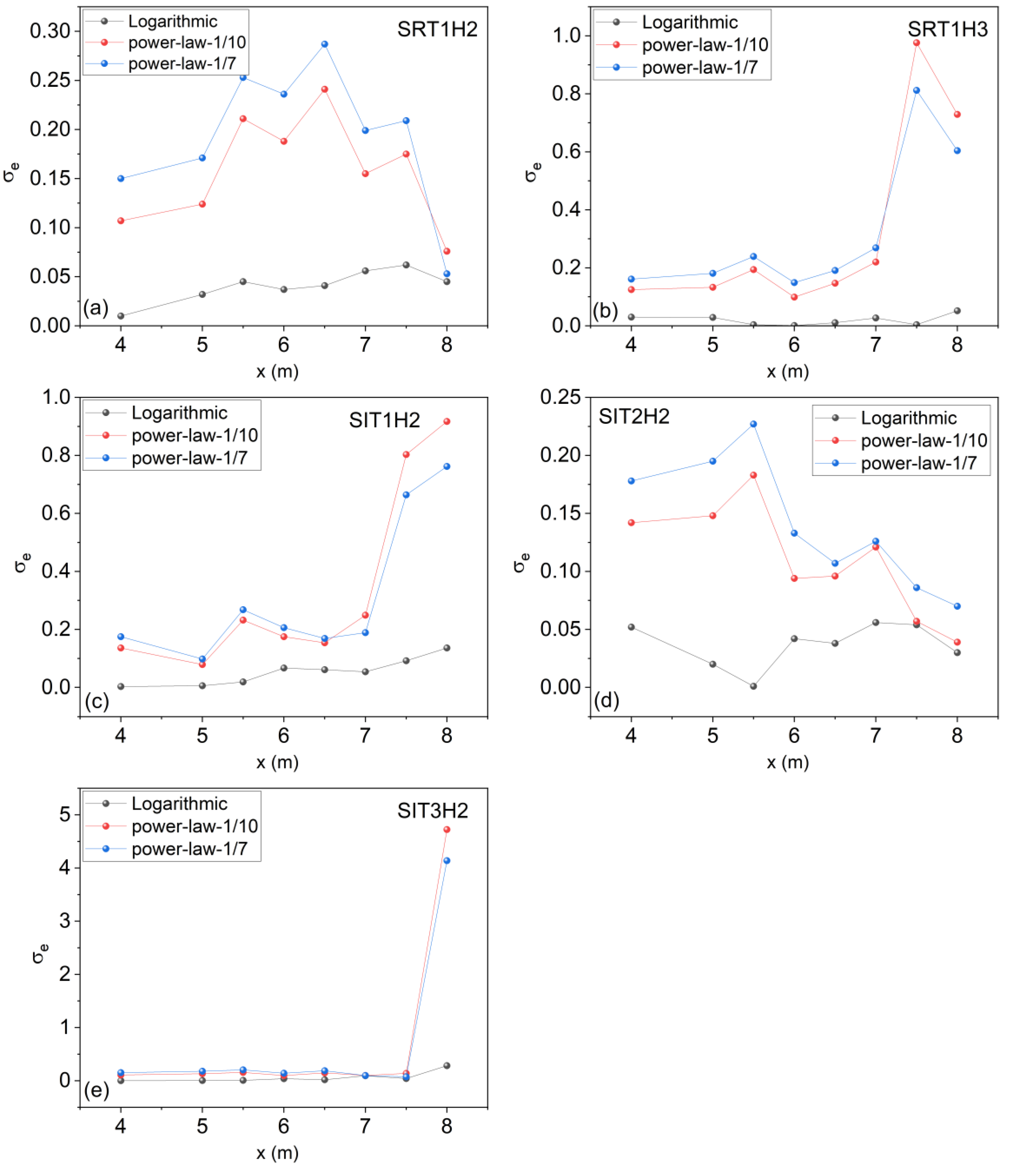
3.2. Distribution Law and Fitting of Offshore Velocity u at Channel Center Position
4. Characteristics of the Vertical Distribution of Rip Current
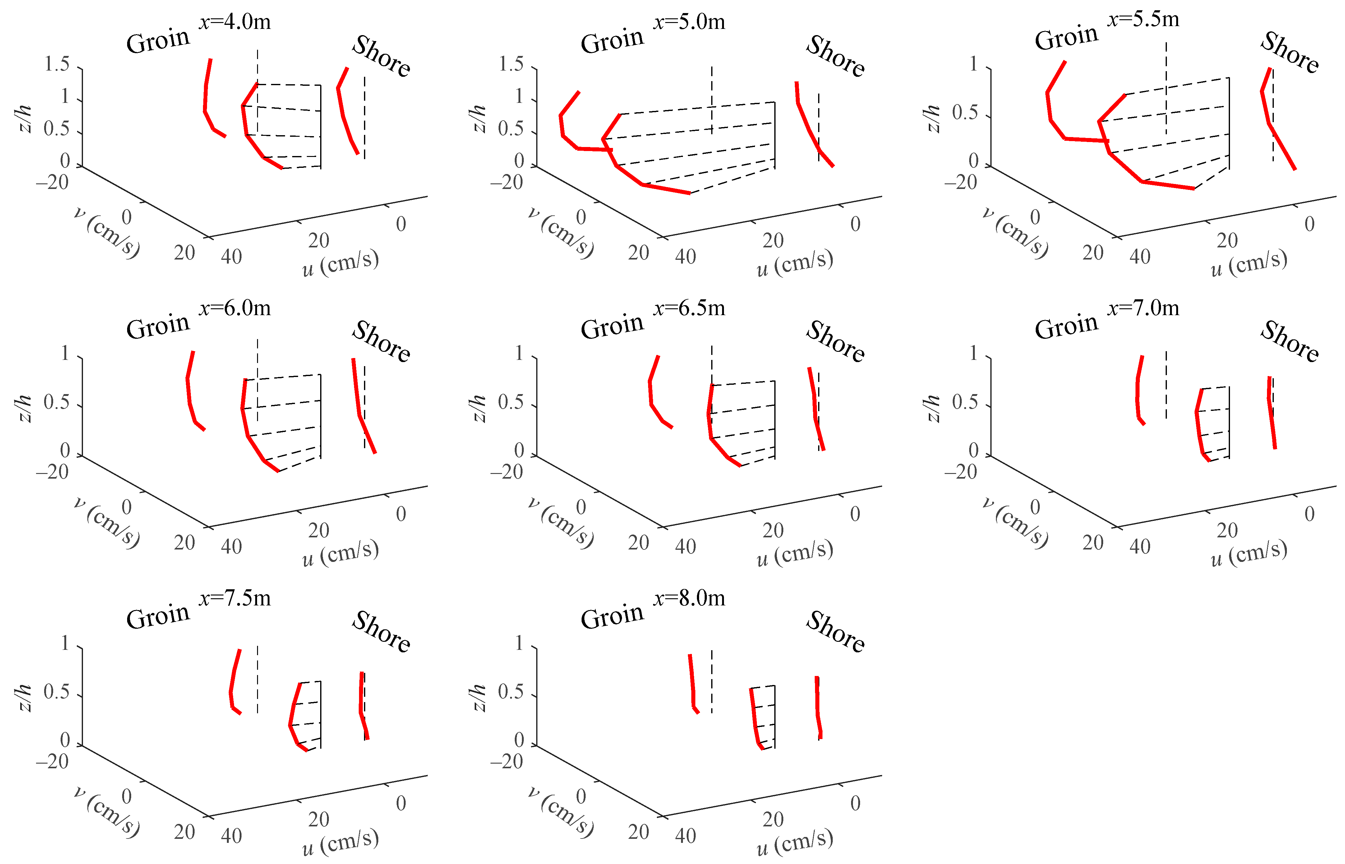
4.1. Vector Characterization of Rip Current
4.2. Influencing Factors of Rip Current
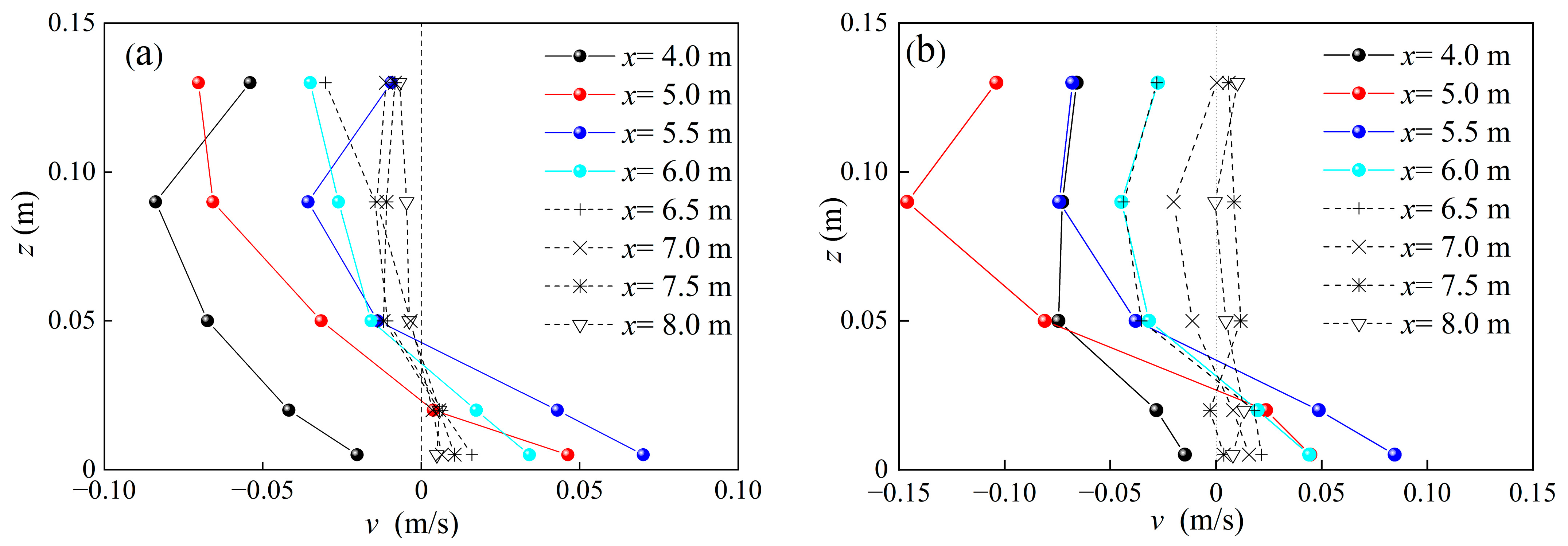
4.2.1. Effect of the Groin on Alongshore Velocity (v)
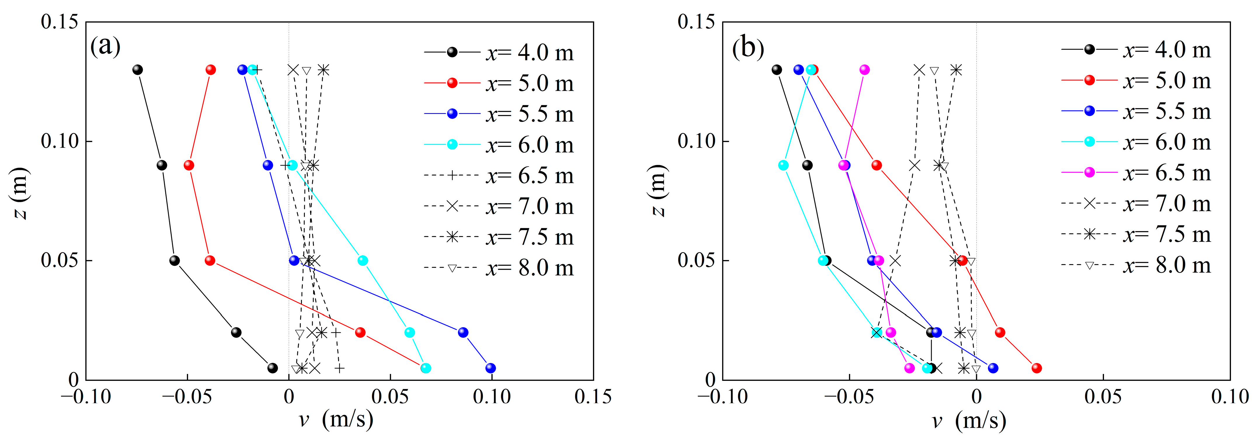
4.2.2. Effect of Wave Period on Alongshore Velocity (v)
4.3. Alongshore Velocity (v) for Different Underwater Topographic Conditions
4.4. Cross-Shore Velocity (u) for Different Underwater Topographic Conditions
5. Discussion
6. Conclusions
- (1)
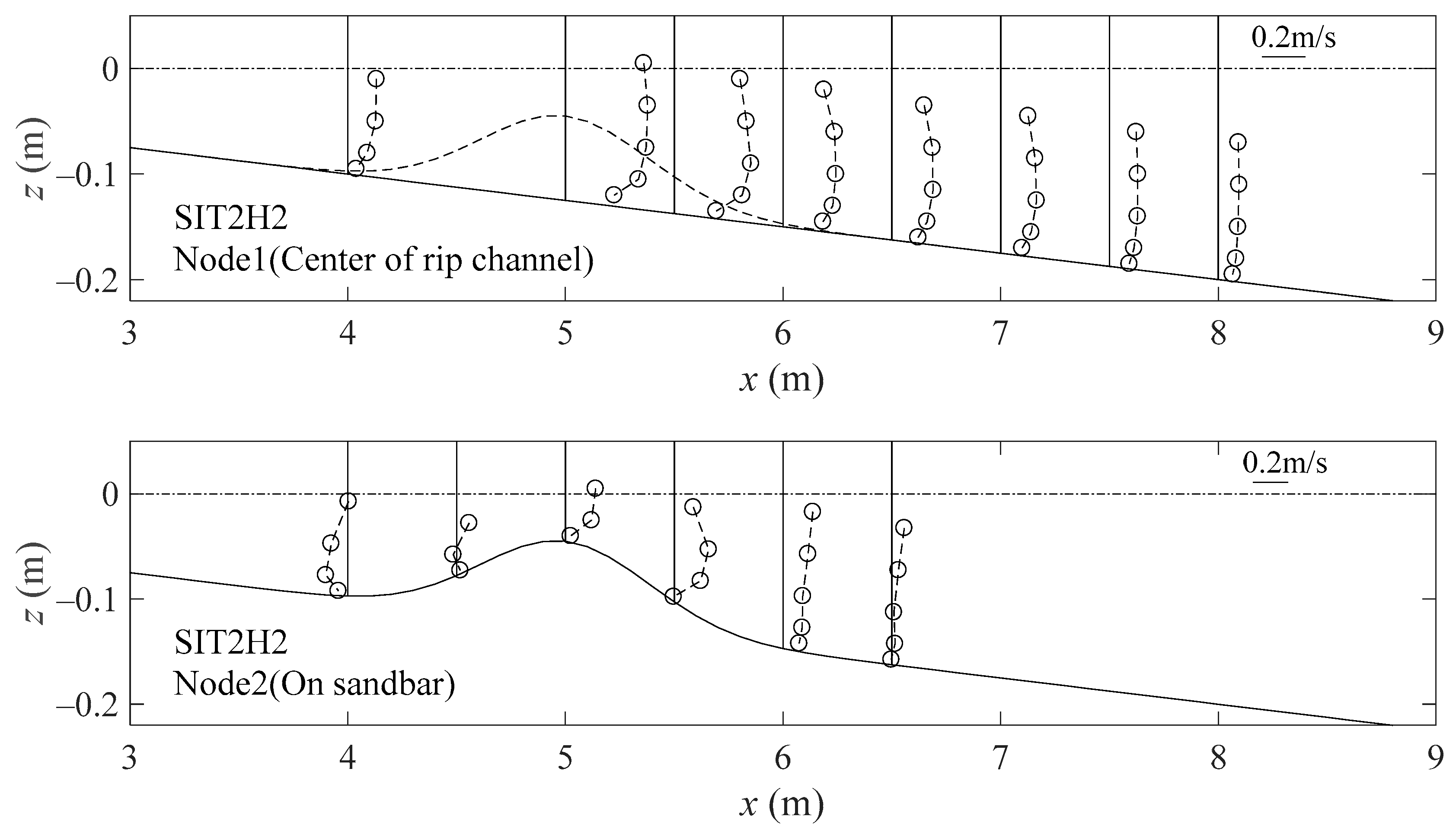
- The vertical variation in the offshore rip current is characterized by the rip current neck being narrower at both ends and wider in the middle, with the rip current head near the water surface exhibiting high-velocity surface flow characteristics. Regarding the rip current neck, it spans two types of terrain: the sandbar and the rip channel. The vertical structure of the rip current along the rip channel’s centerline is more uniform, whereas at the sandbar, it is more variable, being narrower at the ends and wider in the middle. The fitting analysis of the rip current at the rip channel’s centerline indicates that its vertical distribution aligns with the logarithmic distribution law, while an exponential distribution better fits the offshore remote measurement points (x = 7.5 m, 8.0 m) under the SRT2H3 condition with large wave heights.
- (2)
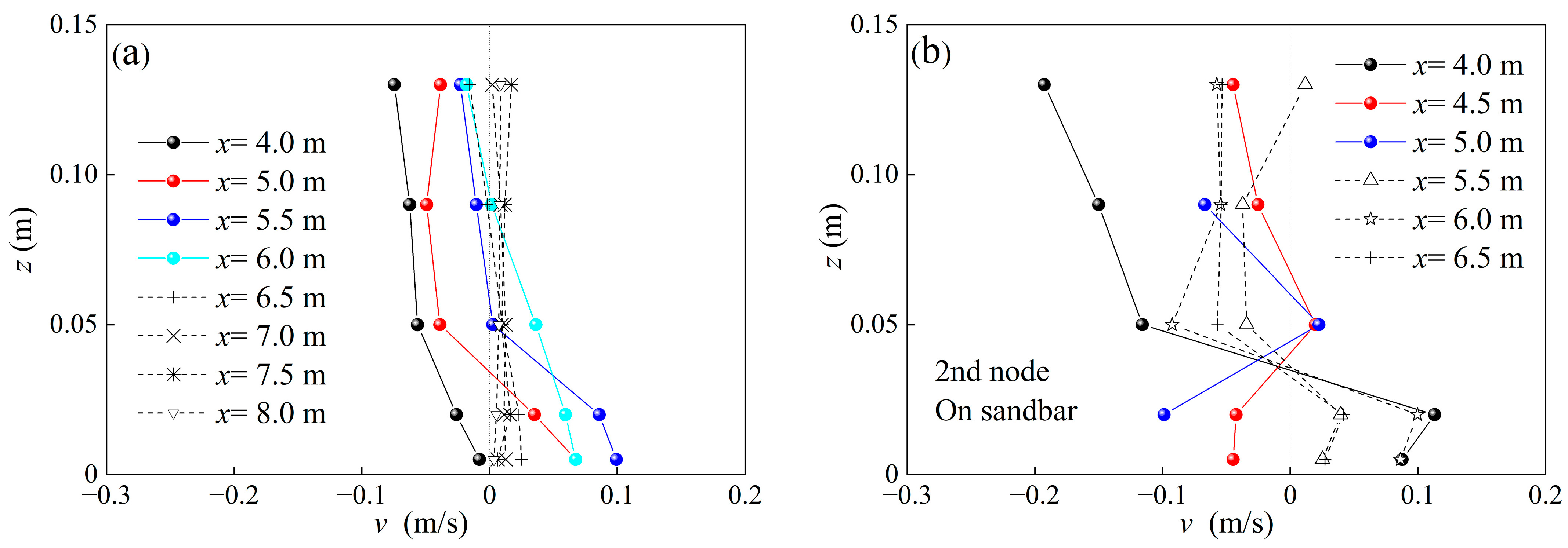
- The alongshore velocity component of a rip current is generally higher at the top and lower at the bottom. For wave conditions with a period of 1.0 s, the current velocity at the uppermost measurement point is marginally lower, yet remains higher than at the bottom, resulting in a trend where the current velocity is larger at mid-depths and smaller nearer the top and bottom. For wave conditions with a period of 1.5 s and 2.0 s, the rip current’s alongshore velocity component exhibits a pattern of being higher at the top and lower at the bottom along the water column.
- (3)
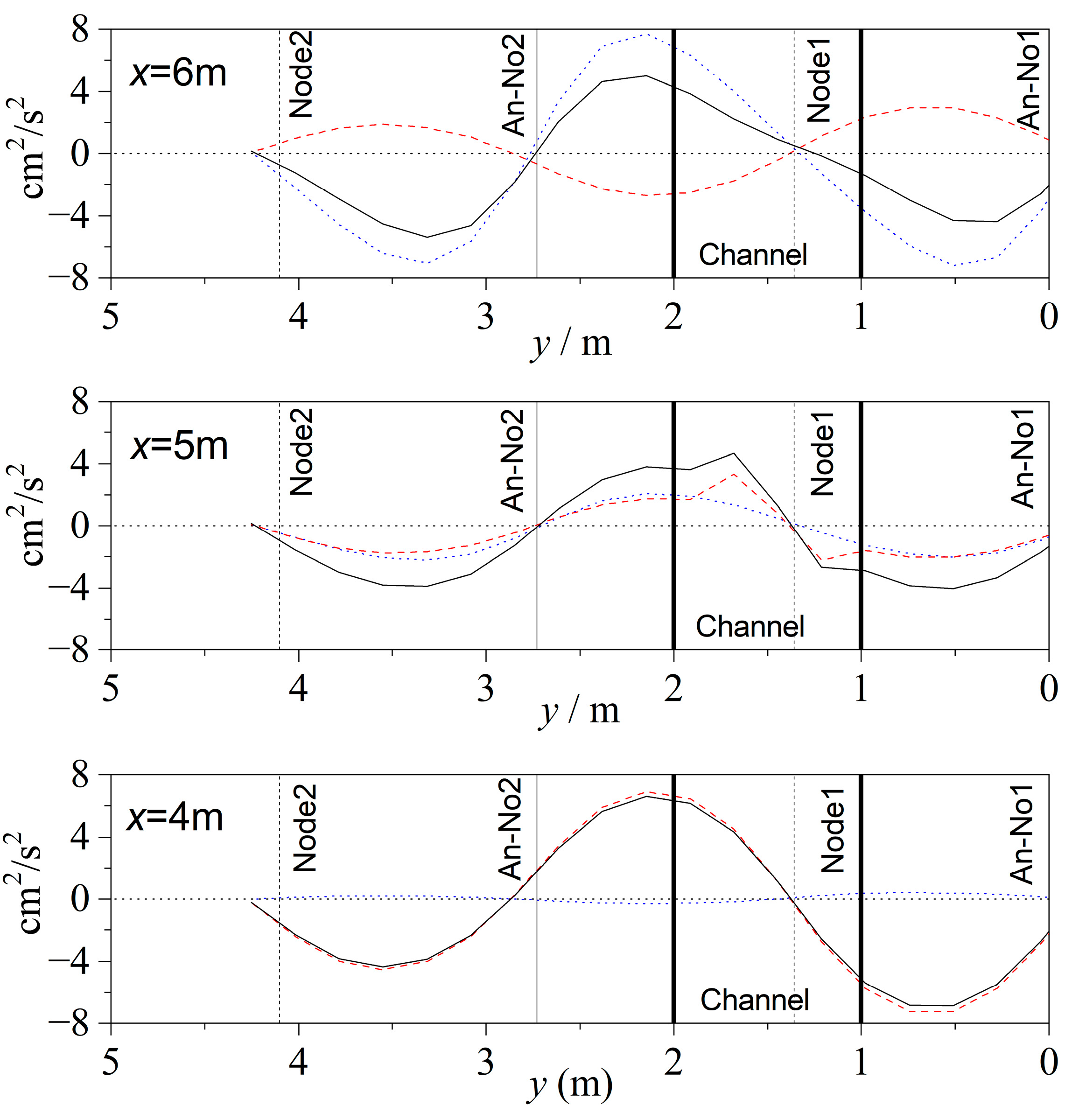
- The alongshore velocity of a rip current fluctuates laterally. The alongshore velocity intensifies with increasing wave height, with its direction being predominantly influenced by the circulation flow. The inclination towards the groin at the rip channel entrance results from the asymmetric circulation flow induced by wave reflection at the groin. The alongshore velocity v at the second node on the sandbar predominantly points towards the groin. This is because the influence of reflected waves is weaker than that of incident waves at this location, farther from the groin. The presence of a channel destroys the symmetry of the incident plus reflected wave pattern and induces an alongshore rip-feeder current on the unbalanced side.
Author Contributions
Funding
Institutional Review Board Statement
Informed Consent Statement
Data Availability Statement
Conflicts of Interest
References
- Dalrymple, R.A.; MacMahan, J.H.; Reniers, A.J.H.M.; Nelko, V. Rip Currents. Annu. Rev. Fluid Mech. 2011, 43, 551–581. [Google Scholar] [CrossRef]
- Castelle, B.; Scott, T.; Brander, R.W.; McCarroll, R.J. Rip Current Types, Circulation and Hazard. Earth-Sci. Rev. 2016, 163, 1–21. [Google Scholar] [CrossRef]
- Hu, P.; Li, Z.; Zhu, D.; Zeng, C.; Liu, R.; Chen, Z.; Su, Q. Field Observation and Numerical Analysis of Rip Currents at Ten-Mile Beach, Hailing Island, China. Estuar. Coast. Shelf Sci. 2022, 276, 108014. [Google Scholar] [CrossRef]
- Stokes, C.; Poate, T.; Masselink, G.; Scott, T.; Instance, S. New Insights into Combined Surfzone and Estuarine Bathing Hazards. EGUsphere 2024, 482, 1–35. [Google Scholar] [CrossRef]
- Lee, J.; Cho, W.C.; Lee, J.L. The Application of a Rip Current Warning Decision-Process System, Haeundae Beach, South Korea. J. Coast. Res. 2016, 75, 1167–1171. [Google Scholar] [CrossRef]
- Sous, D.; Castelle, B.; Mouragues, A.; Bonneton, P. Field Measurements of a High-Energy Headland Deflection Rip Current: Tidal Modulation, Very Low Frequency Pulsation and Vertical Structure. J. Mar. Sci. Eng. 2020, 8, 534. [Google Scholar] [CrossRef]
- Gao, J.L.; Hou, L.H.; Liu, Y.Y.; Shi, H.B. Influences of Bragg Reflection on Harbor Resonance Triggered by Irregular Wave Groups. Ocean Eng. 2024, 305, 117941. [Google Scholar] [CrossRef]
- Haller, M.C.; Dalrymple, R.A.; Svendesen, I.A. Experimental Study of Nearshore Dynamics on a Barred Beach with Rip Channels. J. Geophys. Res. Ocean. 2002, 107, 14-1–14-21. [Google Scholar] [CrossRef]
- Drønen, N.; Karunarathna, H.; Fredsoe, J.; Sumer, B.M.; Deigaard, R. An Experimental Study of Rip Channel Flow. Coast. Eng. 2002, 45, 223–238. [Google Scholar] [CrossRef]
- Xu, J.; Yan, S.; Zou, Z.L.; Chang, C.S.; Fang, K.Z.; Wang, Y. Flow Characteristics of the Rip Current System near a Shore-Normal Structure with Regular Waves. J. Mar. Sci. Eng. 2023, 11, 1297. [Google Scholar] [CrossRef]
- Zhang, Y.; Hong, X.; Qiu, T.; Liu, X.; Sun, Y.; Xu, G. Tidal and Wave Modulation of Rip Current dynamics. Cont. Shelf Res. 2022, 243, 104764. [Google Scholar] [CrossRef]
- Wang, H.; Zhu, S.; Li, X.; Zhang, W.; Nie, Y. Numerical Simulations of Rip Currents off Arc-Shaped Coastlines. Acta Oceanol. Sin. 2018, 37, 21–30. [Google Scholar] [CrossRef]
- Chen, Q.; Dalrymple, R.A.; Kirby, J.T.; Kennedy, A.B.; Haller, M.C. Boussinesq Modeling of a Rip Current System. J. Geophys. Res. Ocean. 1999, 104, 20617–20637. [Google Scholar] [CrossRef]
- Castelle, B.; Michallet, H.; Marieu, V.; Leckler, F.; Dubardier, B.; Lambert, A.; Berni, C.; Bonneton, P.; Barthelemy, E.; Bouchette, F. Laboratory Experiment on Rip Current Circulations over a Moveable Bed: Drifter Measurements. J. Geophys. Res. Ocean. 2010, 115, 17-1–17-17. [Google Scholar] [CrossRef]
- Zheng, J.; Yao, Y.; Chen, S.; Chen, S.; Zhang, Q. Laboratory Study on Wave-Induced Setup and Wave-Driven Current in a 2DH Reef-Lagoon-Channel System. Coast. Eng. 2020, 162, 103772. [Google Scholar] [CrossRef]
- Choi, J.; Roh, M. A Laboratory Experiment of Rip Currents between the Ends of Breaking Wave Crests. Coast. Eng. 2021, 164, 103812. [Google Scholar] [CrossRef]
- Kennedy, A.B.; Thomas, D. Drifter Measurements in a Laboratory Rip Current. J. Geophys. Res. 2004, 109, 1–16. [Google Scholar] [CrossRef]
- MacMahan, J.; Brown, J.; Brown, J.; Thornton, E.; Reniers, A.; Stanton, T.; Henriquez, M.; Gallagher, E.; Morrison, J.; Austin, M.J.; et al. Mean Lagrangian Flow Behavior on an Open Coast Rip-Channeled Beach: A New Perspective. Mar. Geol. 2010, 268, 1–15. [Google Scholar] [CrossRef]
- Gallop, S.L.; Bryan, K.R.; Pitman, S.J.; Ranasinghe, R.; Sandwell, D.; Harrison, S.R. Rip Current Circulation and Surf Zone Retention on a Double Barred Beach. Mar. Geol. 2018, 405, 12–22. [Google Scholar] [CrossRef]
- McCarroll, R.J.; Brander, R.W.; Turner, I.L.; Power, H.E.; Mortlock, T.R. Lagrangian Observations of Circulation on an Embayed Beach with Headland Rip Currents. Mar. Geol. 2014, 355, 173–188. [Google Scholar] [CrossRef]
- Jeong, S.-H.; Kwon, J.H.; Lee, J. Analysis of Rip Current Flow Fields in CCTV Images Using Optimal LSPIV Parameters. J. Coast. Res. 2024, 116, 240–244. [Google Scholar] [CrossRef]
- Sasaki, M. Velocity Profiles in Nearshore Circulation Current. Coast. Eng. Jpn. 1985, 28, 125–136. [Google Scholar] [CrossRef]
- Wind, H.G.; Vreugdenhil, C.B. Rip-Current Generation near Structures. J. Fluid Mech. 1986, 171, 459–476. [Google Scholar] [CrossRef]
- Giger, M.; Dracos, T.; Jirka, G.H. Entrainment and Mixing in Plane Turbulent Jets in Shallow Water. J. Hydraul. Res. 1991, 29, 615–642. [Google Scholar] [CrossRef]
- Haas, K.A.; Svendsen, I.A. Laboratory Measurements of the Vertical Structure of Rip Currents. J. Geophys. Res. Ocean. 2002, 107, 15-1–15-15. [Google Scholar] [CrossRef]
- Poort, M. Rip Currents: A Laboratory Study of a Rip Current in the Presence of a Submerged Reef. Master’s Thesis, Delft University of Technology (TU Delft), Delft, The Netherlands, 2007. [Google Scholar]
- Pattiaratchi, C.; Olsson, D.; Hetzel, Y.; Lowe, R. Wave-Driven Circulation Patterns in the Lee of Groynes. Cont. Shelf Res. 2009, 29, 1961–1974. [Google Scholar] [CrossRef]
- Scott, T.; Austin, M.; Masselink, G.; Russell, P. Dynamics of Rip Currents Associated with Groynes-Field Measurements, Modelling and Implications for Beach Safety. Coast. Eng. 2016, 107, 53–69. [Google Scholar] [CrossRef]
- Dalrymple, R.A. A Mechanism for Rip Current Generation on an Open Coast. J. Geophys. Res. Ocean. 1975, 80, 3485–3487. [Google Scholar] [CrossRef]
- Shin, C.H.; Noh, H.K.; Yoon, S.B.; Choi, J. Understanding of Rip Current Generation Mechanism at Haeundae Beach of Korea: Honeycomb Waves. J. Coast. Res. 2014, 72, 11–15. [Google Scholar] [CrossRef]
- Wei, Z.; Dalrymple, R.A.; Xu, M.; Garnier, R.; Derakhti, M. Short-Crested Waves in the Surf Zone. J. Geophys. Res. Ocean. 2017, 122, 4143–4162. [Google Scholar] [CrossRef]
- Kirby, J.T.; Derakhti, M. Short-Crested Wave Breaking. Eur. J. Mech.—B/Fluids 2019, 73, 100–111. [Google Scholar] [CrossRef]
- Baker, C.M.; Moulton, M.; Palmsten, M.L.; Brodie, K.; Nuss, E.; Chickadel, C.C. Remotely Sensed Short-Crested Breaking Waves in a Laboratory Directional Wave Basin. Coast. Eng. Jpn. 2023, 183, 104327. [Google Scholar] [CrossRef]
- Long, J.W.; Özkan-Haller, H.T. Offshore Controls on Nearshore Rip Currents. J. Geophys. Res. Ocean. 2005, 110, 21-1–21-21. [Google Scholar] [CrossRef]
- Zhang, Y.; Shi, F.; Kirby, J.T.; Feng, X. Phase-Resolved Modeling of Wave Interference and Its Effects on Nearshore Circulation in a Large Ebb Shoal-Beach System. J. Geophys. Res. Ocean. 2022, 127, e2022JC018623. [Google Scholar] [CrossRef]
- Dalrymple, R.A.; Lanan, G.A. Beach Cusps Formed by Intersecting Waves. Geol. Soc. Am. Bull. 1976, 87, 57–60. [Google Scholar] [CrossRef]
- Svendsen, I.A. Introduction to Nearshore Hydrodynamics; World Scientific: Singapore, 2006. [Google Scholar]
- Dyer, K.R. Current Velocity Profiles in a Tidal Channel. Geophys. J. R. Astron. Soc. 1971, 22, 153–161. [Google Scholar] [CrossRef]
- Barenblatt, G.I. Scaling Laws for Fully-Developed Turbulent Shear Flows. 1. Basic Hypotheses and Analysis. J. Fluid Mech. 1993, 248, 513–520. [Google Scholar] [CrossRef]
- Faria, A.F.G.; Thornton, E.B.; Stanton, T.P.; Soares, C.K.; Lippmann, T.C. Vertical profiles of Longshore Currents and Related Bed Shear Stress and Bottom Roughness. J. Geophys. Res. 1998, 103, 3217–3232. [Google Scholar] [CrossRef]
- Wang, Y.; Zhang, Z.; Zou, Z.; Liu, Z. Rip Currents by Intersecting Wave on Barred Beach with Rip Channel. Adv. Water Sci. 2019, 30, 760–768. [Google Scholar] [CrossRef]
- Wang, Y.; Zou, Z. Experimental Study of Rip Currents by Intersecting Wave on Barred Beach. Adv. Water Sci. 2015, 26, 123–129. [Google Scholar] [CrossRef]
- Zhang, Z.-W.; Zou, Z.-L. Vertical Distribution of Longshore Currents over Plane and Barred Beaches. J. Hydrodyn. Ser. B 2012, 24, 718–728. [Google Scholar] [CrossRef]
- Zhang, Z.-W.; Zou, Z.-L. Application of Power Law to Vertical Distribution of Longshore Currents. Water Sci. Eng. 2019, 12, 73–83. [Google Scholar] [CrossRef]
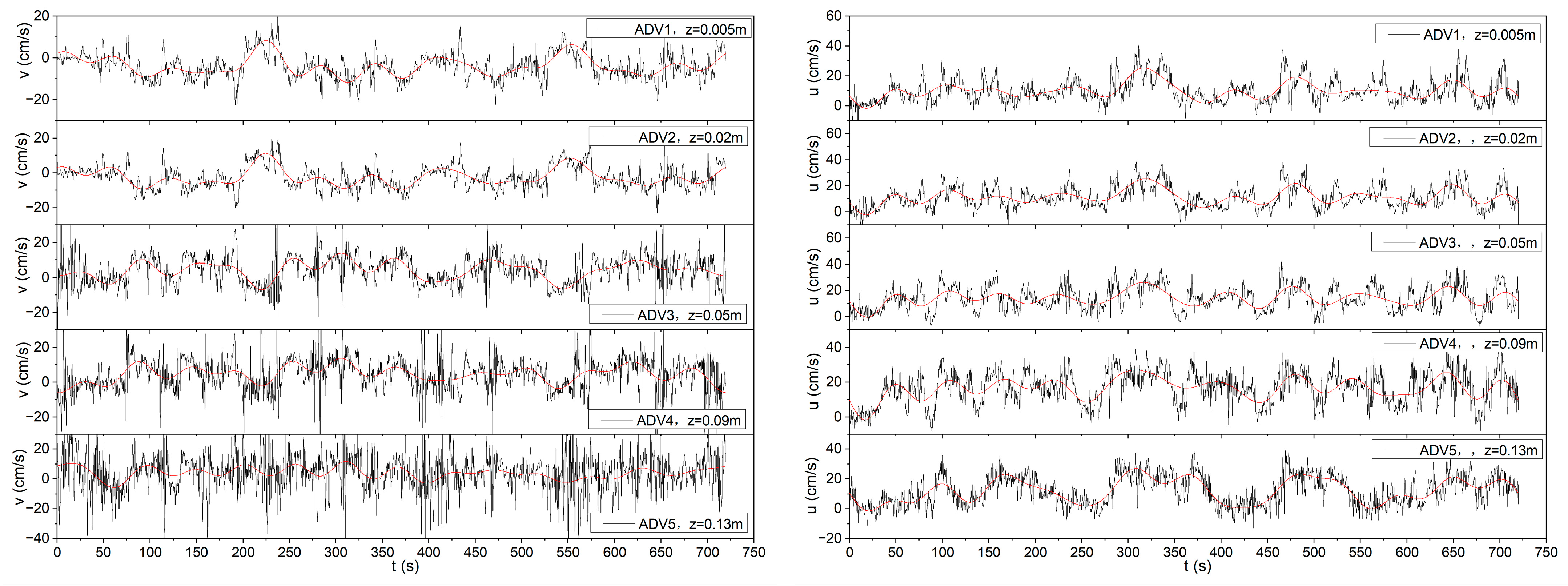
 : ADV velocity
  : float velocity (
 : 20 cm/s).
: ADV velocity : float velocity (: 20 cm/s).
: 20 cm/s).
: ADV velocity : float velocity (: 20 cm/s).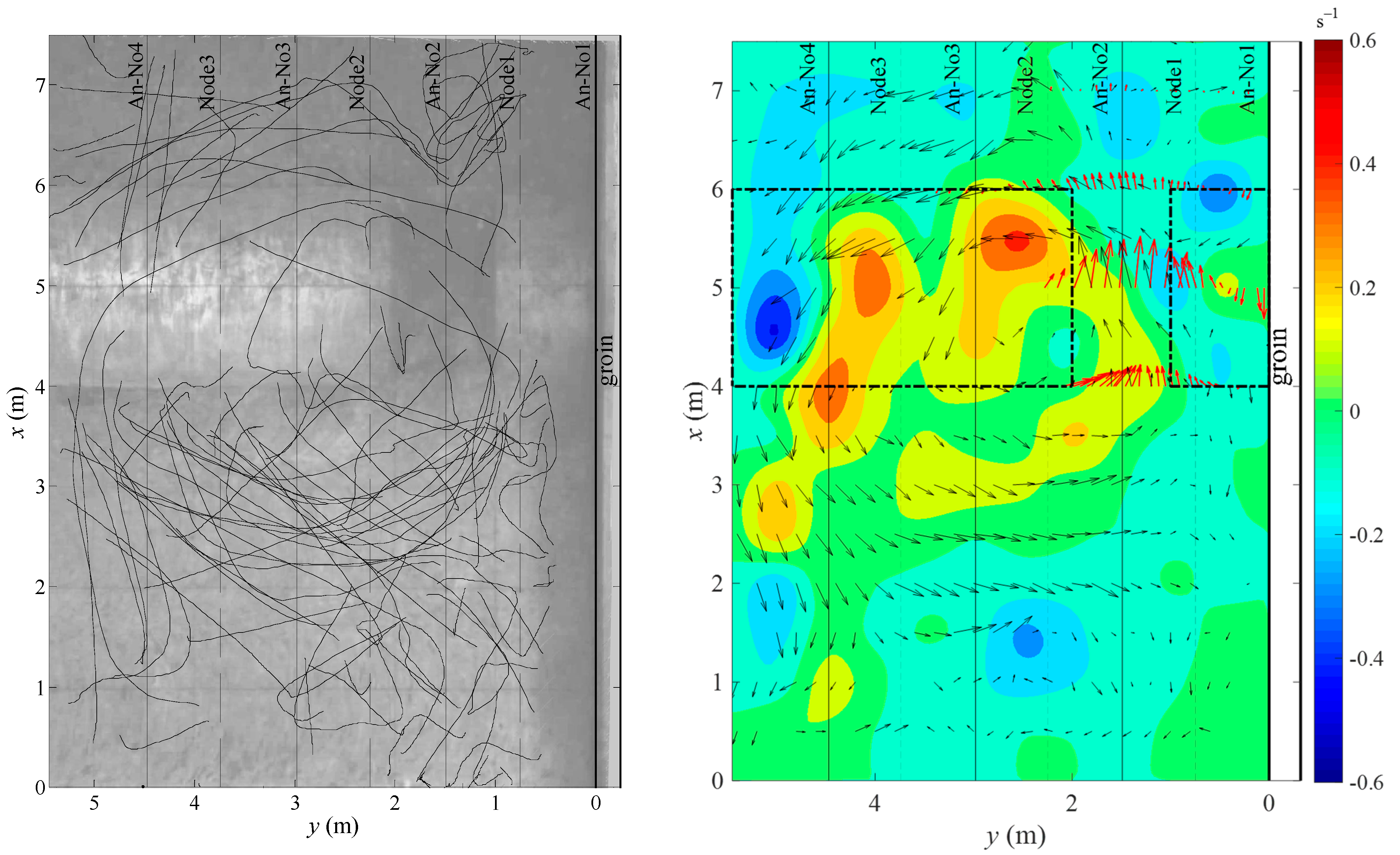


| Case | Wave Type | Wave Height (cm) | Wave Period (s) | Wave Breaking Point (m) | (m) | Node | Antinode | Node/Anti-Node Points Relative Position of Rip Channel | |||||
|---|---|---|---|---|---|---|---|---|---|---|---|---|---|
| Antinode Outside of Channel | Rip Channel | 1 | 2 | 3 | 1 | 2 | 3 | ||||||
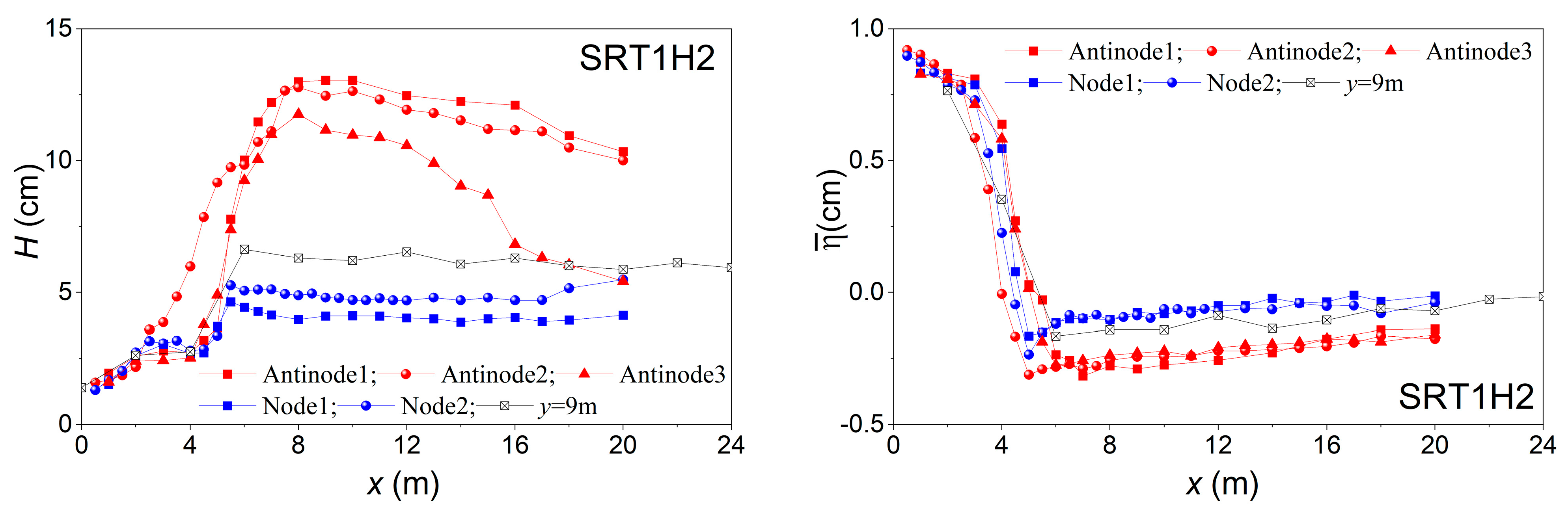
| SRT1H2 | regular | 5.80 | 1.0 | 7.0 | 8.0 | 1.50 | 0.75 | 2.25 | 3.74 | 0 | 1.50 | 2.98 | coincides with the 2nd antinode |
| SRT1H3 | regular | 6.98 | 1.0 | 8.5 | 9.0 | ||||||||
| SIT1H2 | Irregular | 4.53 | 1.0 | 7.0 | 7.0 | ||||||||
| SIT2H2 | Irregular | 4.84 | 1.5 | 7.0 | 5.5 | 2.73 | 1.41 | 4.14 | 6.87 | 0 | 2.73 | 5.46 | close to the 1st node |
| SIT3H2 | Irregular | 4.68 | 2.0 | 7.5 | 5.5 | 3.88 | 1.94 | 5.82 | 9.70 | 0 | 3.88 | 7.76 | between the 1st antinode point and the 1st node |
| Case | x/m | Hrms/m | Logarithmic Fitting | Power-Law Fitting | |||||
|---|---|---|---|---|---|---|---|---|---|
| a | b | m | m | ||||||
| SRT1H2 | 4.0 | 0.043 | −22.89 | 163.68 | 0.010 | 1/10 | 0.107 | 1/7 | 0.150 |
| 5.0 | 0.050 | −18.39 | 43.45 | 0.032 | 1/10 | 0.124 | 1/7 | 0.171 | |
| 5.5 | 0.081 | −15.26 | 43.84 | 0.045 | 1/10 | 0.211 | 1/7 | 0.253 | |
| 6.0 | 0.086 | −22.32 | 118.66 | 0.037 | 1/10 | 0.188 | 1/7 | 0.236 | |
| 6.5 | 0.089 | −16.33 | 91.57 | 0.041 | 1/10 | 0.241 | 1/7 | 0.287 | |
| 7.0 | 0.086 | −15.40 | 189.26 | 0.056 | 1/10 | 0.155 | 1/7 | 0.199 | |
| 7.5 | 0.092 | −10.35 | 126.24 | 0.062 | 1/10 | 0.175 | 1/7 | 0.209 | |
| 8.0 | 0.092 | −10.91 | 180.97 | 0.045 | 1/10 | 0.076 | 1/7 | 0.053 | |
| SRT1H3 | 4.0 | 0.034 | −12.63 | 72.87 | 0.030 | 1/10 | 0.125 | 1/7 | 0.161 |
| 5.0 | 0.050 | −32.03 | 82.73 | 0.029 | 1/10 | 0.133 | 1/7 | 0.181 | |
| 5.5 | 0.069 | −29.81 | 82.95 | 0.004 | 1/10 | 0.194 | 1/7 | 0.239 | |
| 6.0 | 0.081 | −13.40 | 57.68 | 0.001 | 1/10 | 0.099 | 1/7 | 0.149 | |
| 6.5 | 0.100 | −10.95 | 63.18 | 0.011 | 1/10 | 0.147 | 1/7 | 0.191 | |
| 7.0 | 0.110 | −16.01 | 104.46 | 0.027 | 1/10 | 0.220 | 1/7 | 0.269 | |
| 7.5 | 0.111 | −7.29 | 118.13 | 0.004 | 1/10 | 0.976 | 1/7 | 0.812 | |
| 8.0 | 0.115 | −9.35 | 224.47 | 0.052 | 1/10 | 0.729 | 1/7 | 0.604 | |
| SIT1H2 | 4.0 | 0.032 | −19.40 | 186.57 | 0.003 | 1/10 | 0.136 | 1/7 | 0.175 |
| 5.0 | 0.043 | −10.23 | 31.28 | 0.006 | 1/10 | 0.079 | 1/7 | 0.098 | |
| 5.5 | 0.05 | −10.75 | 43.05 | 0.019 | 1/10 | 0.232 | 1/7 | 0.268 | |
| 6.0 | 0.050 | −11.14 | 98.56 | 0.067 | 1/10 | 0.175 | 1/7 | 0.206 | |
| 6.5 | 0.054 | −8.84 | 105.72 | 0.061 | 1/10 | 0.154 | 1/7 | 0.169 | |
| 7.0 | 0.055 | −7.26 | 108.87 | 0.054 | 1/10 | 0.249 | 1/7 | 0.189 | |
| 7.5 | 0.057 | −6.09 | 109.71 | 0.092 | 1/10 | 0.803 | 1/7 | 0.664 | |
| 8.0 | 0.057 | −5.91 | 136.07 | 0.136 | 1/10 | 0.917 | 1/7 | 0.762 | |
| SIT2H2 | 4.0 | 0.040 | −13.68 | 78.50 | 0.052 | 1/10 | 0.142 | 1/7 | 0.178 |
| 5.0 | 0.045 | −37.81 | 91.31 | 0.020 | 1/10 | 0.148 | 1/7 | 0.195 | |
| 5.5 | 0.051 | −19.28 | 46.23 | 0.001 | 1/10 | 0.183 | 1/7 | 0.227 | |
| 6.0 | 0.049 | −13.27 | 43.12 | 0.042 | 1/10 | 0.094 | 1/7 | 0.133 | |
| 6.5 | 0.049 | −10.04 | 38.76 | 0.038 | 1/10 | 0.096 | 1/7 | 0.107 | |
| 7.0 | 0.047 | −9.26 | 39.88 | 0.056 | 1/10 | 0.121 | 1/7 | 0.126 | |
| 7.5 | 0.045 | −11.94 | 73.39 | 0.054 | 1/10 | 0.057 | 1/7 | 0.086 | |
| 8.0 | 0.043 | −12.40 | 106.34 | 0.030 | 1/10 | 0.039 | 1/7 | 0.070 | |
| SIT3H2 | 4.0 | 0.046 | −31.22 | 122.37 | 0.001 | 1/10 | 0.109 | 1/7 | 0.152 |
| 5.0 | 0.046 | −31.76 | 73.78 | 0.005 | 1/10 | 0.132 | 1/7 | 0.179 | |
| 5.5 | 0.048 | −22.50 | 57.55 | 0.007 | 1/10 | 0.156 | 1/7 | 0.204 | |
| 6.0 | 0.042 | −15.23 | 47.17 | 0.038 | 1/10 | 0.098 | 1/7 | 0.141 | |
| 6.5 | 0.044 | −18.38 | 95.58 | 0.019 | 1/10 | 0.147 | 1/7 | 0.188 | |
| 7.0 | 0.042 | −9.44 | 74.58 | 0.094 | 1/10 | 0.100 | 1/7 | 0.099 | |
| 7.5 | 0.042 | −8.89 | 126.46 | 0.042 | 1/10 | 0.139 | 1/7 | 0.075 | |
| 8.0 | 0.037 | −5.37 | 133.88 | 0.283 | 1/10 | 4.724 | 1/7 | 4.139 | |
Disclaimer/Publisher’s Note: The statements, opinions and data contained in all publications are solely those of the individual author(s) and contributor(s) and not of MDPI and/or the editor(s). MDPI and/or the editor(s) disclaim responsibility for any injury to people or property resulting from any ideas, methods, instructions or products referred to in the content. |
© 2024 by the authors. Licensee MDPI, Basel, Switzerland. This article is an open access article distributed under the terms and conditions of the Creative Commons Attribution (CC BY) license (https://creativecommons.org/licenses/by/4.0/).
Share and Cite
Wang, Y.; Zou, Z.; Liu, Z.; Song, M. Vertical Distribution of Rip Currents Generated by Intersecting Waves in a Sandbar–Groin Systems. J. Mar. Sci. Eng. 2024, 12, 911. https://doi.org/10.3390/jmse12060911
Wang Y, Zou Z, Liu Z, Song M. Vertical Distribution of Rip Currents Generated by Intersecting Waves in a Sandbar–Groin Systems. Journal of Marine Science and Engineering. 2024; 12(6):911. https://doi.org/10.3390/jmse12060911
Chicago/Turabian StyleWang, Yan, Zhili Zou, Zhongbo Liu, and Meixia Song. 2024. "Vertical Distribution of Rip Currents Generated by Intersecting Waves in a Sandbar–Groin Systems" Journal of Marine Science and Engineering 12, no. 6: 911. https://doi.org/10.3390/jmse12060911