Numerical Investigation into the Stability of Offshore Wind Power Piles Subjected to Lateral Loads in Extreme Environments

Abstract

Monopile foundations are extensively utilized in the rapidly expanding offshore wind power industry, and the stability of these foundations has become a crucial factor for ensuring the safety of offshore wind power projects. Such foundations are subjected to a myriad of complex environmental loads during their operational lifespan. Whilst current research predominantly concentrates on the effects of wind, wave, and current loads on monopile stability in extreme environments, it is imperative to consider the potential influence of unexpected submarine landslide loads. In this study, we provide a comprehensive overview of wind, wave, current, and submarine landslide loads on monopile foundations in extreme environments. Subsequently, we establish a finite element model for analyzing the stability of monopiles under complex lateral loads, and validate the accuracy of the model by comparing it with the previous numerical findings. A case study is performed with reference to the Xiangshui Wind Farm project to analyze the effects of varying submarine landslide densities, velocities, impact heights, and seabed sediment strengths on pile head horizontal displacement, pile rotation at the mudline, and maximum bending moment. The findings indicate that the increase in submarine landslide density, velocity, and impact height leads to an increase in horizontal displacement at the pile head, pile rotation at the mudline, and maximum bending moments, and a horizontal failure mode is observed in seabed sediments. Furthermore, under the same load conditions, a decrease in seabed sediment strength and internal friction angle triggers instability in monopiles, with a noteworthy transition from horizontal failure to deep-seated seabed sediment failure. Finally, we propose a criterion for monopile instability under diverse loading conditions.

1. Introduction

Wind energy is a widely adopted renewable energy source and plays a pivotal role in the development of offshore wind power resources. In recent years, offshore wind projects have been rapidly emerging as modern scientific research has paid increasing attention to sustainable development and efficient use of resources. This growth is attributed to the abundant wind energy resources and broader installation areas available in the marine environment, as well as their minimal impact on human activities [1,2,3,4]. According to the Global Offshore Wind Report 2023 [5], the global installed capacity of offshore wind power reached 64.3 GW by the end of 2022, with 8.8 GW of newly installed capacity. Mainland China accounted for a significant share of 57.6%, followed by the United Kingdom and Taiwan. Forecasts indicate a continuous annual increase in global offshore wind power installation capacity over the next decade. It is estimated that 15.45 GW of additional offshore wind capacity will be installed globally by 2023, with a cumulative total of 60.2 GW expected to be installed in the next 10 years.

Currently, pile foundations are widely employed in offshore wind power projects due to their robust adaptability to geological conditions, simple structure, convenient design and manufacturing, and ease of construction [6]. However, damages to pile foundations during the operation of offshore wind power projects have been reported, which is attributed to the influence of complex loads [7]. Consequently, ensuring the stability of pile foundations becomes a critical prerequisite for project safety. Current research on the stability of offshore pile foundation primarily focuses on the external dynamic loads acting on the piles, including wind, waves, and currents. Zeng et al. [8] investigated the effect of breaking waves on the monopile foundation of offshore wind turbines on the slope edge by utilizing laboratory experiments and computational fluid dynamics models. It was found that, during wave breaking, the pressure acting on the monopile exhibited a wave-like distribution with a gradual decrease in the point of action. Shi et al. [9] developed a “three-stage” computational model for monopile foundation of offshore wind turbines to investigate force conditions in soil, water, and air. They derived the total dynamic impedance of the foundation to predict its dynamic response, and analyzed tower displacement under various monopile parameters. Miles et al. [10] conducted a series of laboratory experiments to analyze the coupled effects of waves and currents as well as to study the influence of these factors on the monopile foundation of offshore wind turbines. Ong et al. [11] performed dynamic analysis on offshore monopile under the influence of sea currents using a finite element model. They examined the response of monopiles under wind–wave coupling conditions in shallow water with varying parameters. Buljac et al. [12] conducted experiments on a small-scale wind turbine in a wind–wave–current tank, and investigated the combined effects of wind, waves, and currents on the monopile foundation of offshore wind turbines. It was found that, among the overall loads acting on the offshore wind turbine, the longitudinal oscillating force induced by currents dominated. Achmus et al. [13] established a calculation model for the interaction between waves, wind turbines, and seabed foundations. They simplified wind–wave loads into concentrated horizontal forces acting on the top of the tower to study the horizontal bearing characteristics of offshore wind power monopile foundations. Wu et al. [14] employed finite element analysis to study high-pile foundations for offshore wind power, and they also simulated the evolution of the load-bearing capacity of wind power foundations under varying soil strength parameters. The results indicated that improved soil, increased burial depth, and a larger pile diameter effectively enhanced the load-bearing capacity of pile foundation.

Previous studies have predominantly focused on assessing the effects of wind, waves, and currents on the stability of pile foundation. However, in recent years, given the frequent occurrence of extreme storms and geological events worldwide [15], attention has shifted towards understanding the effect of incidental loads, such as submarine landslides, on pile foundations. Submarine landslides are manifest as localized or widespread seabed instability, significant deformations, and sliding phenomena [16,17,18]. High-speed submarine landslides can cause considerable damage to marine structures with unidirectional impact loads [19,20,21]. For instance, the 1929 Grand Banks landslide in Canada travelled at a speed of up to 20 m/s, leading to the destruction of 12 seabed pipelines [22,23,24,25]. The 2006 submarine landslide in the Luzon Strait severed 11 seabed communication cables, resulting in prolonged communication interruptions [26]. Currently, research on the influence of submarine landslides on piles is primarily concentrated on the quantification of the impact loads of submarine landslides. Li et al. [27] conducted 12 experiments in a submarine landslide model trough and optimized the formula for a dimensionless resistance coefficient acting on pile foundations by adjusting variables such as the slope of the model trough and the mass fraction of kaolin clay in the landslide body. Li et al. [28] employed computational fluid dynamics to study the impact force of submarine debris flows on the monopile and analyzed the characteristics of the drag force acting on the monopile. Li et al. [16] simulated the impact of submarine debris flows on pile foundations using computational fluid dynamics and proposed a formula for predicting impact forces. However, whilst these studies have analyzed the impact forces of submarine landslides on pile foundations, they have not explored whether pile foundations would be unstable and the instability mechanism after exposure to the impact loads of submarine landslides. Simultaneously, the stability of pile foundations under the combined effects of submarine landslides, wind, waves, currents, and other complex loads still lacks in-depth exploration, and there is an urgent need for further research in this regard.

This study develops a finite element model to investigate the interaction between piles and soil under complex lateral loading conditions. The accuracy of the model is validated through finite element simulation cases from previous studies. Subsequently, based on a quantification equation for submarine landslide impact loads established by previous researchers, the study determines the lateral loads experienced by a monopile under the coupled effects of submarine landslides, wind, waves, and currents in complex environments. Finally, the stability analysis of a monopile under complex lateral loading conditions is conducted by considering different seabed sediment strengths, and the stability of monopile foundations is discussed in detail.

2. Numerical Model

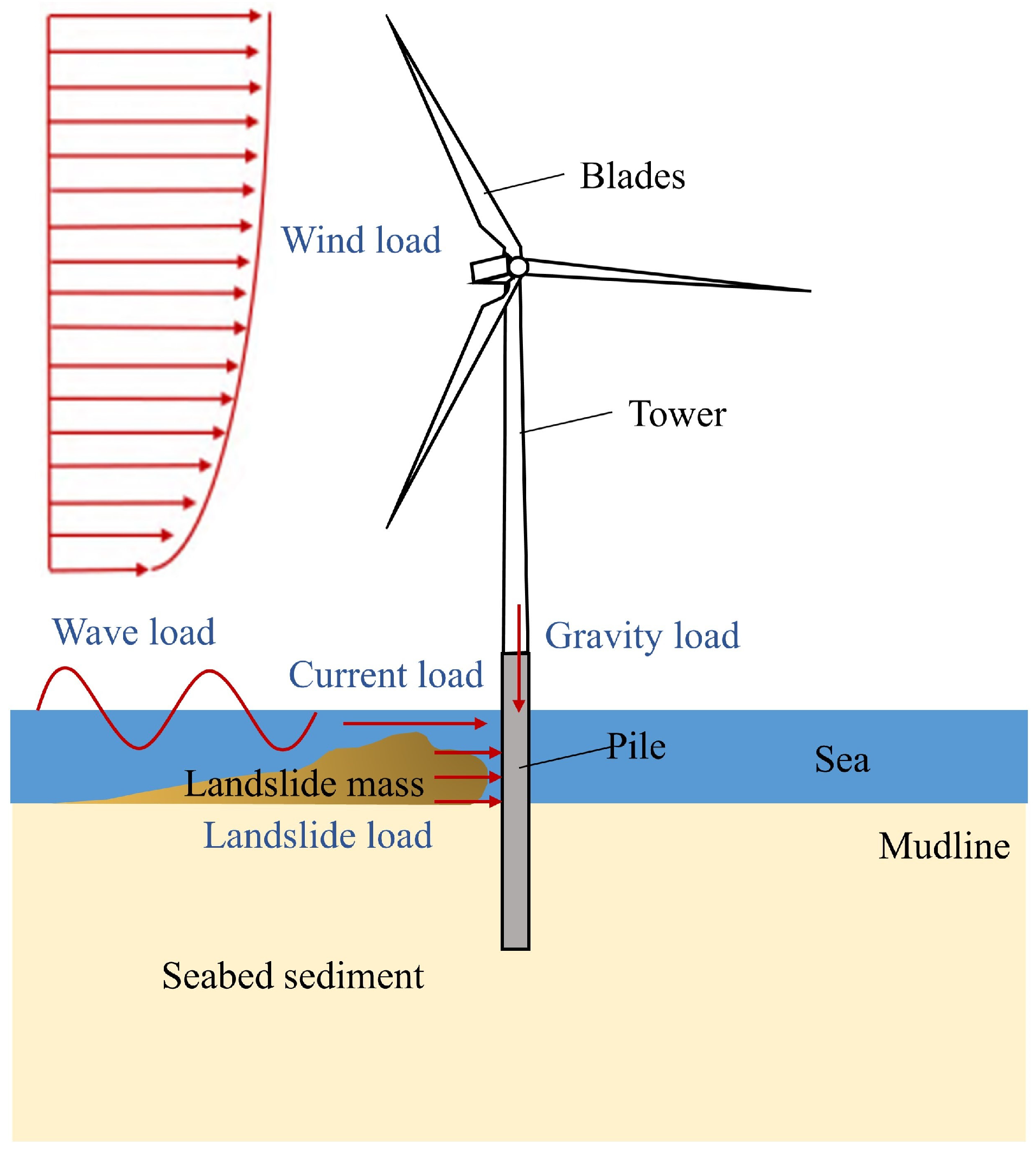
2.1. Generalization of Loads on Offshore Wind Turbine Structures in Complex Environments

In the marine environment, offshore wind turbine structures are exposed to wind, waves, and currents throughout their operational lifespan. Additionally, they may encounter sporadic loads such as landslides, as depicted in Figure 1. Specifically, the wind exerts forces on the blades and hub of the turbine, while the tower (the upper section of the monopile) is exposed to wave and current loads. Furthermore, the pile foundation may experience occasional loads from seabed landslides. Clearly, the structure of offshore wind turbines is subject to a complex interaction of forces. To facilitate analysis, current research often simplifies these dynamic loads to horizontal forces acting on individual pile foundations. Subsequently, investigations focused on the stability of monopile foundations under the combined influence of these horizontal loads [13,29,30].

2.1.1. Aerodynamic Loads

The aerodynamic loads acting on offshore wind turbines can be categorized into blade wind load and tower load. Blade wind load is the wind-induced force experienced by the entire rotor blades of the turbine, constituting the primary load factor. Meanwhile, tower load represents the wind force acting on the tower structure exposed to the air. Given the relatively smaller dimensions of the tower, the magnitude of this load is comparably smaller. The blade wind load can be simplified as follows [31]:

$$F_a=\frac{1}{2}{\rho }_a{A}_R{C}_T{U}^2,$$

(1)

where $F_a$ is the wind load on blades; ${\rho }_a$ is the density of air, ${\rho }_a=1.225$ kg/m³; $A_R$ is the rotor swept area, which is calculated according to the size of the blade; $C_T$ is the coefficient of thrust; and $U$ is the wind speed. Considering the different ranges of wind speed, the thrust coefficient can be approximated as three different segments over the operational range of the turbine:

When cut-in wind speed ($U_{in}$) ≤ wind speed ($U$) ≤ the rated wind speed ($U_R$), the impeller thrust coefficient is calculated as follows [32]:

$$C_T=\frac{3.5\left(2U_R+3.5\right)}{{U_R}^2},$$

(2)

When the rated wind speed ($U_R$) ≤ wind speed ($U$) ≤ cut-out wind speed ($U_{out}$), the calculation formula for the impeller thrust coefficient is as follows:

$$C_T=3.5U_R\left(2U_R+3.5\right)\cdot \frac{1}{U^3},$$

(3)

When the wind speed is low, Equation (2) will overestimate the thrust coefficient when assuming that the impeller thrust coefficient does not exceed 1, so its value is limited to 1.

The diameter of the tower structure is small relative to the wind range, and its influence on the wind flow is negligible, so the wind load acting on the tower is calculated according to the following formula [33]:

$$F_t=\frac{1}{2}{\rho }_a{U}^2\left(Z\right)C_{s}D,$$

(4)

where $F_t$ is the wind load of the tower; $C_s$ is the coefficient of drag force for wind, which is dimensionless and is not affected by the specific size of the object, but is only related to the shape of the structure. In engineering, it is used to represent the resistance characteristics of the movement of the object, and the tower is a cylindrical section, which can be taken as 0.5 after calculation; and $D$ is the diameter of pile. According to the wind resistance design code [34], the exponential formula for simulating the change in average wind speed along the height is as follows:

$$\frac{U\left(Z\right)}{U\left(Z_1\right)}={\left(\frac{Z}{Z_1}\right)}^{\alpha },$$

(5)

where $U\left(Z_1\right)$ is the average wind speed at the standard height $Z_1$, which is generally 10 m, and $\alpha$ is the wind shear index, $\alpha =0.143$.

2.1.2. Hydrodynamic Loads

Hydrodynamic loads that include wave and current forces are known as wave–current coupled loads. According to the Code for Design of Wind Turbine Foundations for Offshore Wind Power Projects (NB/T10105-2018) [35], a simplified approach for wave loading involves the Morison equation [36]. This equation decomposes wave forces into two components. One is proportional to acceleration and represents the inertial force, while the other one is proportional to the square of velocity and symbolizes drag force. The formulation is as follows:

$$F_W=F_D+F_I=\frac{1}{2}{C}_D{\rho }_{s}A\overrightarrow{U}\left|\overrightarrow{U}\right|+C_M\rho V_0\overrightarrow{U},$$

(6)

where $F_W$ is the wave load; $F_D$ is the drag force term; $F_I$ is the inertial force term; $A$ is the projected area per unit beam height perpendicular to the wave propagation direction; $V_0$ is the volume of drainage per unit cylinder height; ${\rho }_s$ is the density of seawater and ${\rho }_s=1025$ kg/m³; $C_D$ is the coefficient of drag force perpendicular to the axis of the cylinder, which reflects the viscous effect caused by the viscosity of the fluid; and $C_M$ is the coefficient of inertial force. According to the Code of Hydrology for Harbour (JTJ213-98) [37], the cylinder under the action of wave and current loads can take $C_D=1.2$ and $C_M=2.0$. $\overrightarrow{U}$ is the wave velocity.

For current loads, the current is idealized as a uniform motion, so it does not produce acceleration at the water quality point. Only the inertial force term in the Morison’s formula is omitted, and only the drag force term is calculated [38]:

$$F_C=\frac{1}{2}{C}_W{\rho }_{s}A\overrightarrow{U}\left|\overrightarrow{U}\right|,$$

(7)

where $F_C$ is the current load; and $C_W$ is the coefficient of drag force for current, $C_W=0.73$.

2.1.3. Submarine Landslide Impact Loads

For the impact force of submarine landslides acting on structures, Feng et al. [39] varied the content of kaolin and silt to produce submarine debris flows with diverse rheological properties and densities. Then, they experimentally simulated the influence of these debris flows on model piles. By integrating fluid mechanics theory, they developed an expression that correlates the drag coefficient with the Reynolds number of non-Newtonian fluids.

$$F_L=\frac{1}{2}{C}_d{\rho }_L{v}^{2}hD,$$

(8)

where $F_L$ is the landslide load; $C_d$ is the coefficient of drag force for landslide; ${\rho }_L$ is the debris flow density of submarine landslides; $v$ is the flow velocity of the landslide; $h$ is the impact height of submarine landslides; and $D$ is the diameter of pile.

The drag coefficient can be used to measure the magnitude of the impact force. According to the principles of fluid mechanics, the drag coefficient is closely related to the Reynolds number. The relationship between the drag coefficient and the Reynolds number was fitted [39] as follows:

$$C_d=0.87+\frac{4.71}{{\mathit{Re}}^{0.57} },$$

(9)

The Reynolds number of non-Newtonian fluids is often expressed as follows:

$$\mathit{Re}=\frac{{\rho }_L\cdot v^2}{\mu \cdot \stackrel{.}{\gamma }}=\frac{{\rho }_L\cdot v^2}{\tau },$$

(10)

where $\stackrel{.}{\gamma }$ is the shear rate of the near-pile slurry; $\mu$ is the debris flow viscosity; and $\tau$ is the shear stress. The relationship between fluid shear stress and shear rate can be described by the Herschel–Bulkley model [40]. Feng et al. [39] used the rheometer to test the rheological parameters of the slurry, and obtained the expression of the rheological curve:

$$\tau =0.5+1.5{\stackrel{.}{\gamma }}^{0.42},$$

(11)

where $\stackrel{.}{\gamma }=\frac{v}{D}$.

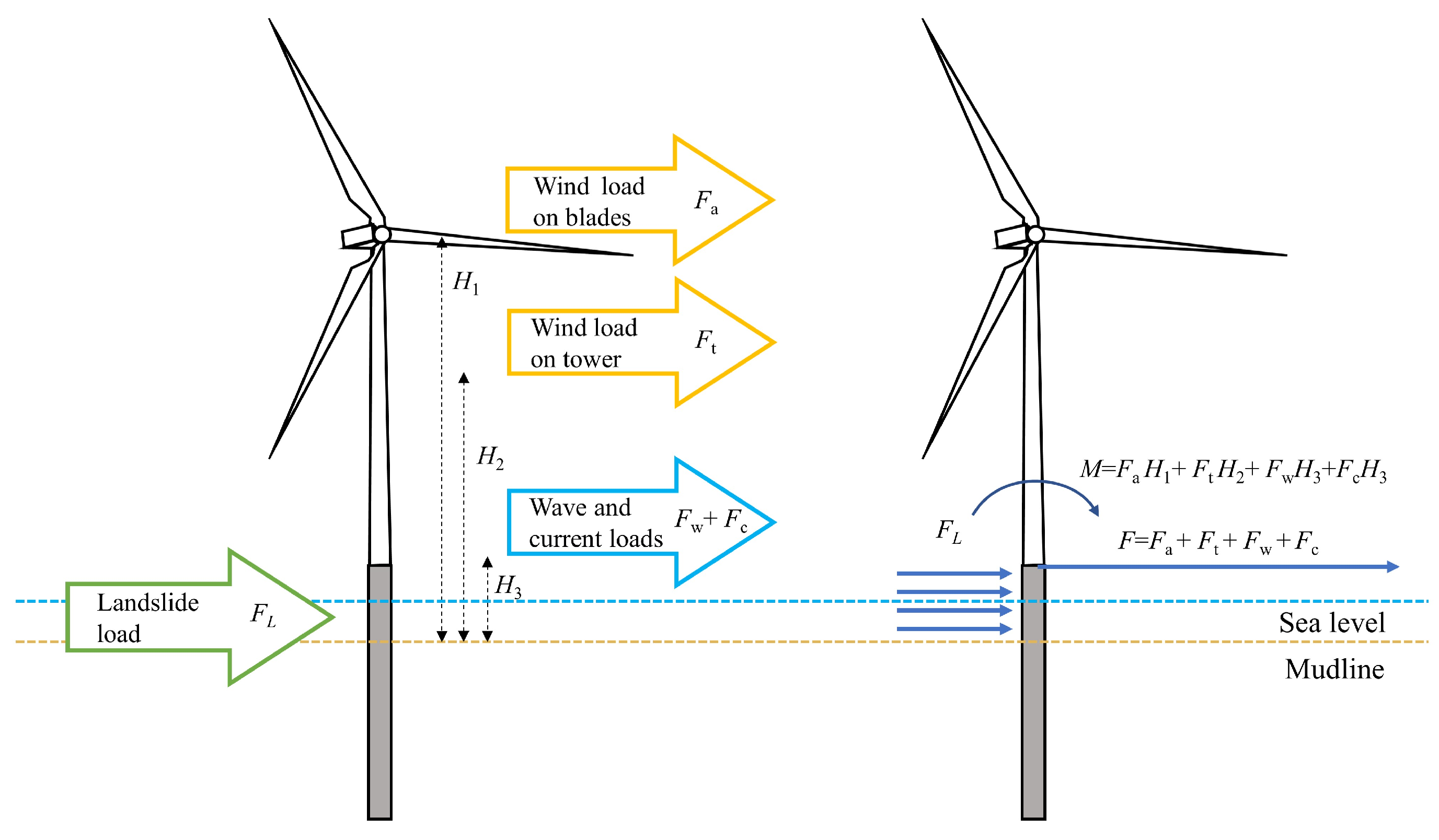
2.1.4. Superimposition of Environmental Loads

For simplicity, this study simplifies the analysis of horizontal loads acting on offshore wind turbines, as depicted in Figure 2. The figure depicts wind load on blades, wind load on tower, wave load, current load, and landslide load, and their respective impact zones. Given the distinctive structural design of offshore wind turbines, the primary load on the foundation piles is manifested as an overturning moment. Various environmental loads can be equivalently represented as horizontal loads and moments applied at the same elevation, as illustrated in Figure 2. Submarine landslides apply loads to the sides of the pile through uniformly distributed forces.

2.2. Pile–Soil Interaction Model under Complex Horizontal Loads

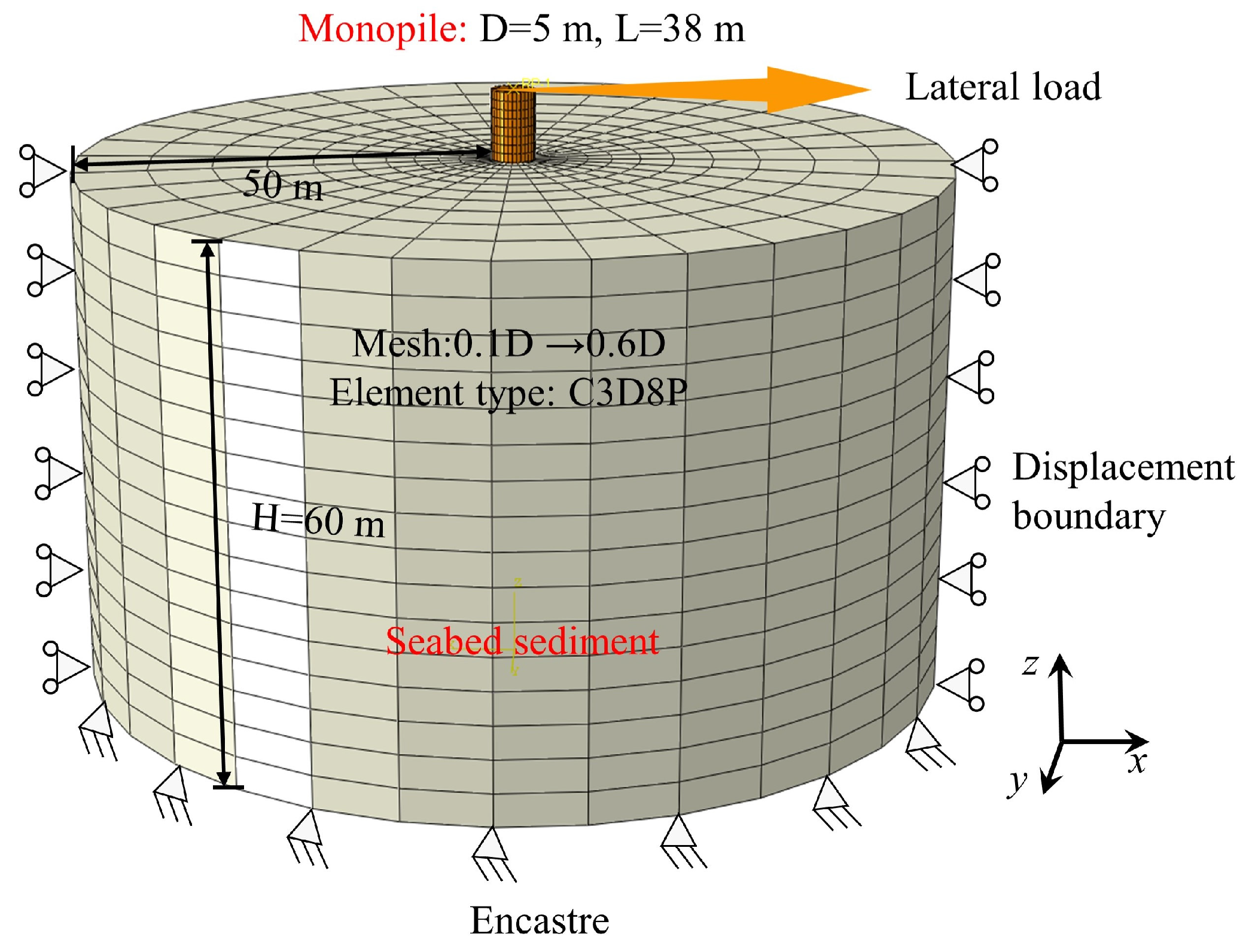
2.2.1. Monopile Model

To solve the pile body displacement and stress at the pile head under horizontal loading, based on the beam bending theory, an element analysis method is employed. Lai [41] selected a differential element of length $dz$ along the horizontal loaded pile, and derived the following equation through the equilibrium of bending moments:

$$(M+dM)-M+P_{z}dy+Sdz=0,$$

(12)

According to the beam theory:

$$\frac{d^{2}M}{d{z}^2}=E_p{I}_p\frac{d^{4}y}{d{z}^4},$$

(13)

The governing equations for the horizontal load of the pile can be obtained immediately by the combination of two formulas:

$$E_p{I}_p\frac{d^{4}y}{d{z}^4}+P_z\frac{d^{2}y}{d{z}^2}+p=0,$$

(14)

where $p=\frac{dS}{dz}$ is the earth reaction force. The essence of calculating the horizontal load response of the pile foundation by the finite element method is to solve the governing equation of the horizontally loaded pile.

An isotropic elastic model is adopted for the monopile, and the stress–strain relationship of the pile material is modelled by Hooke’s law. Hooke’s law in three dimensions can be expressed as follows:

$$\left[\begin{array}{c}{\sigma }_{xx}\\ {\sigma }_{yy}\\ {\sigma }_{zz}\\ {\sigma }_{xy}\\ {\sigma }_{yz}\\ {\sigma }_{zx}\end{array}\right]=\frac{E}{\left(1-2\upsilon \right)\left(1+\upsilon \right)}\left[\begin{array}{cccccc}1-\upsilon & \upsilon & \upsilon & 0& 0& 0\\ \upsilon & 1-\upsilon & \upsilon & 0& 0& 0\\ \upsilon & \upsilon & 1-\upsilon & 0& 0& 0\\ 0& 0& 0& \frac{1}{2}-\upsilon & 0& 0\\ 0& 0& 0& 0& \frac{1}{2}-\upsilon & \frac{1}{2}-\upsilon \end{array}\right]\left[\begin{array}{c}{\epsilon }_{xx}\\ {\epsilon }_{yy}\\ {\epsilon }_{zz}\\ {\gamma }_{xy}\\ {\gamma }_{yz}\\ {\gamma }_{zx}\end{array}\right],$$

(15)

where $E$ is Young’s modulus and $\upsilon$ is the Poisson’s ratio.

2.2.2. Soil Model

The Mohr–Coulomb model can describe the elastoplastic characteristics of soil to some extent, and is widely applied in lateral load pile models [42]. The simulation of the soil in this paper adopts the elastoplastic Mohr–Coulomb model, which can effectively assess the effect of landslide surges. The model mainly involves the following parameters, i.e., the cohesion $c$, the friction angle $\phi$, Young’s modulus $E$, Poisson’s ratio $\upsilon$, and the dilation angle $\psi$. According to Johnson [43], the failure envelope only depends on the principal stress (${\sigma }_1,{\sigma }_3$) and not on the medium principal stress (${\sigma }_2$). When mapped to a three-dimensional stress space, the Mohr–Coulomb theory is decomposed into irregular hexagonal pyramids. This pyramid forms a destruction/yield envelope, and these determine the behavior of the soil. When the stress point is located in the envelope surface, the material undergoes elastic deformation; and when the stress reaches the yield surface, the material will undergo plastic deformation. In this study, it is assumed that the soil has a linear elastic relationship before failure.

2.2.3. Pile–Soil Contact Model

The “contact pair” algorithm is used to simulate the interaction between pile and soil through defining the normal and tangential contact. The discretization method of the surface adopts the “face-to-face contact”, which allows the geometry of the master and slave surfaces to be considered simultaneously. The shear stress and normal pressure of the contact surface are calculated with high accuracy. The “hard” contact option is used for normal contact, while the Coulomb contact is used for tangential contact. The interface shear stress is calculated as follows [44]:

$${\tau }_f={\sigma }_n^{\prime }{\mathit{tan\delta }}_{\mathit{cs}}$$

(16)

where ${\tau }_f$ is the shear stress of the contact surface; ${\sigma }_n^{\prime }$ is the normal effective stress; ${\delta }_{cs}$ is the friction angle of the pile–soil interface in the critical state. The tracking of the relative movement of the contact surface adopts “finite sliding”, and the calculation accuracy is improved by continuously determining whether the master and slave surfaces are in contact.

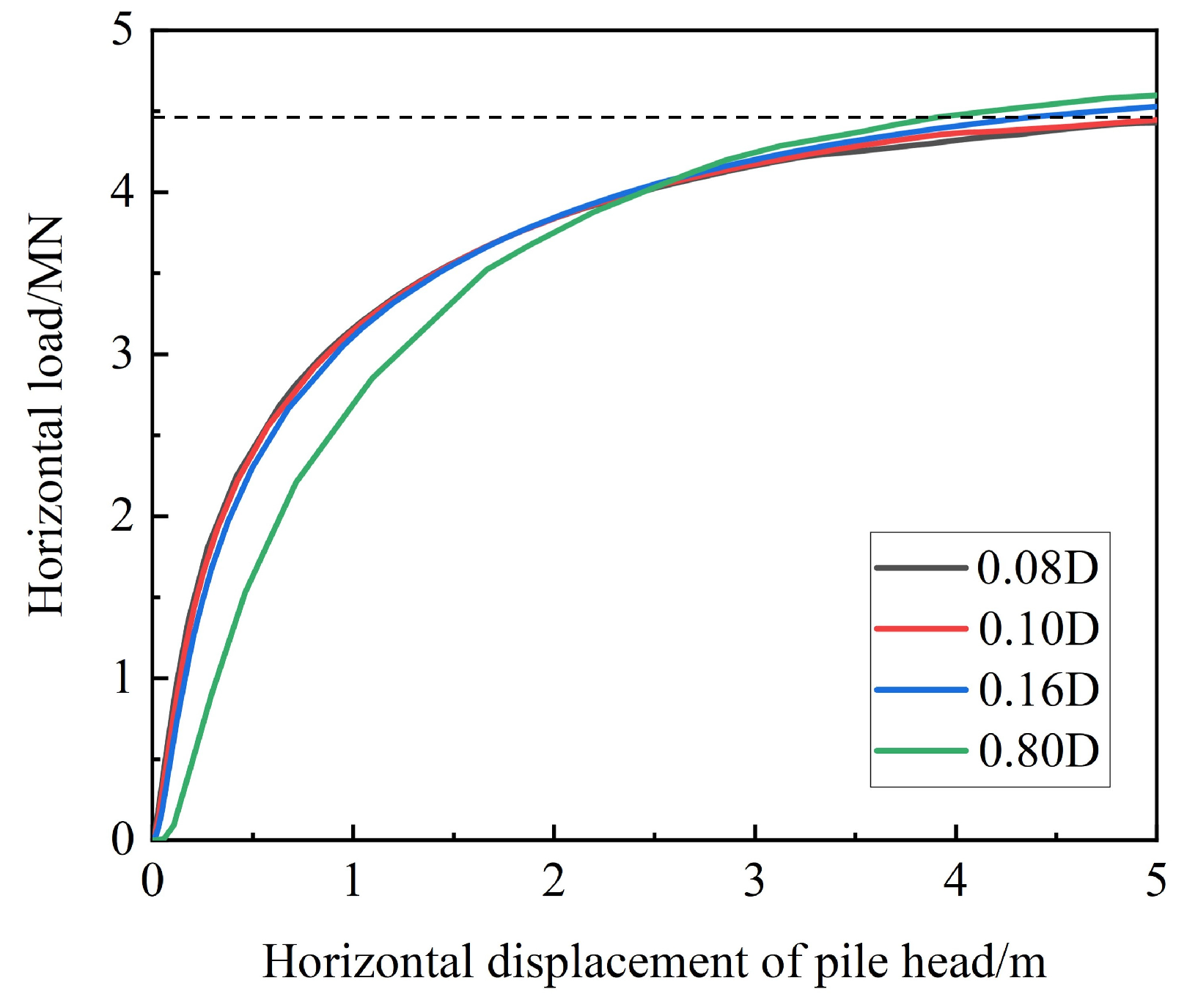
2.2.4. Finite Element Method for Solution

Finite element method is a mathematical approximation of the actual physical system. The analyzed object is subdivided into simple and interacting tiny units, and all of which together form a mechanical system. It treats the solution domain as a composition of many small interconnected subdomains and gives an approximate solution to each subdomain. Finally, the approximate solutions of all subdomains satisfy the corresponding equilibrium conditions, leading to the final solution [45].

In this study, computational analysis is performed using the standard solver module of ABAQUS software that can simulate most of the material and geometric nonlinear problems. The Newton–Raphson method is usually used to solve the ABAQUS/standard nonlinear response, and the principle of this method is described below. The equilibrium equation for a structure or soil at a given time is as follows:

$$I\left(u\right)-P\left(u\right)=0,$$

(17)

where $I$ is the internal force of the finite element node at that moment; $P$ is the external load on the finite element node at that time; and $u$ is the displacement of the node at that time. Assuming that $r$ is a displacement correction, after $i$ iterations, there is:

$$I\left(u_i+r_{\mathrm{i}+1}\right)-P\left(u_i+r_{\mathrm{i}+1}\right)=0,$$

(18)

where $r_{\mathrm{i}+1}=u_{\mathrm{i}+1}-u_i$. Expand $I\left(u_i+r_{\mathrm{i}+1}\right)-P\left(u_i+r_{\mathrm{i}+1}\right)$ Taylor near $u_i$, and the higher-order terms are omitted:

$$I(u_i)-P(u_i)=(\frac{\partial P(u_i)}{\partial u}-\frac{\partial I(u_i)}{\partial u})r_{i+1},$$

(19)

Similarly, the following equation can be obtained:

$$I(u_{i+1})-P(u_{i+1})=(\frac{\partial P(u_{i+1})}{\partial u}-\frac{\partial I(u_{i+1})}{\partial u})r_{i+2},$$

(20)

The total load is expressed as follows:

$$P_T-I\left(u_{i+1}\right)=R_{i+1},$$

(21)

where $P_T$ is the total load and $R_{i+1}$ is the residual. ABAQUS will iterate until $R_{i+1}$ is within the set tolerance.

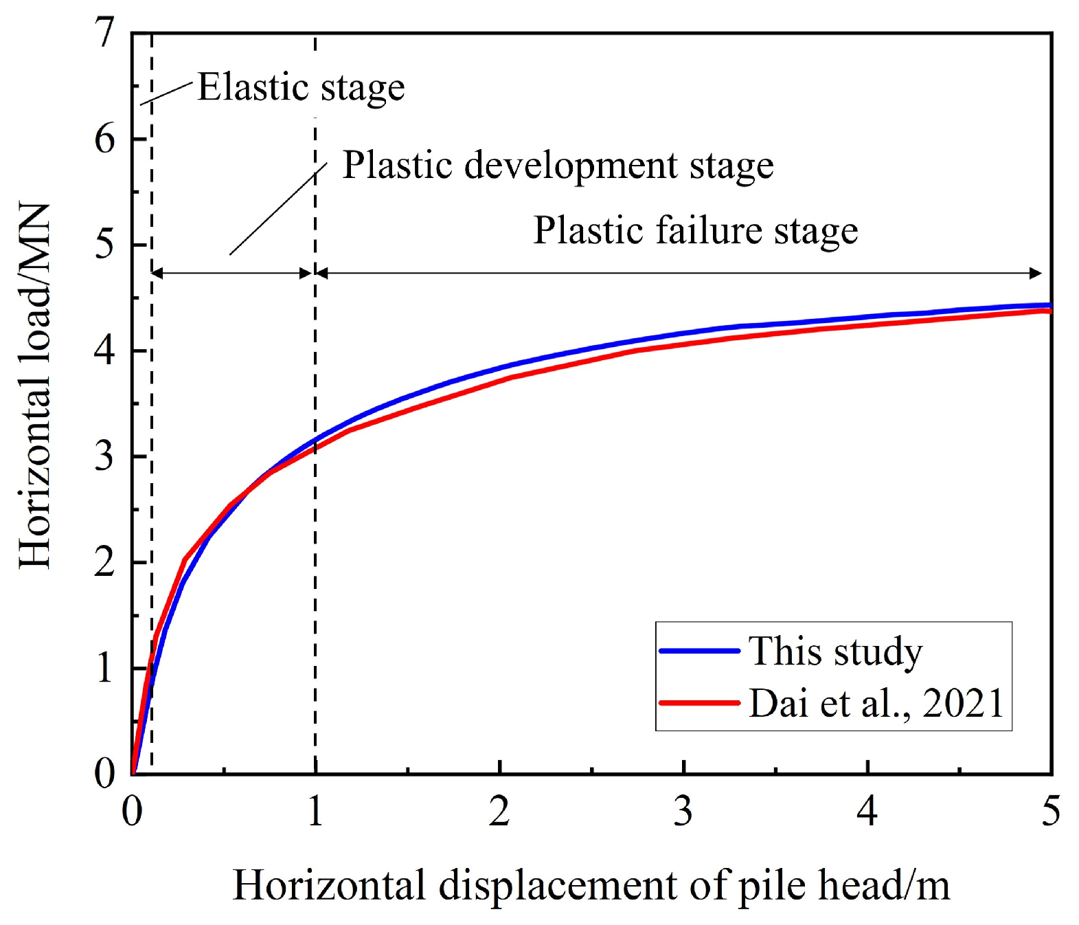
2.3. Numerical Model Verification

We utilize the stability analysis of large-diameter monopile foundations under horizontal load conducted by Dai et al. [46] as a case study to verify the effectiveness of the proposed numerical model. In this case, the single pile had a diameter of 5 m and a total length of 38 m, and a buried depth of 30 m. For offshore wind turbine applications, the monopile foundation is considered as a hollow steel pipe pile, which is equivalent to a solid rigid pile based on flexural stiffness assumptions. This ensures consistent load-bearing capacity and failure modes [46]. The equivalent elastic modulus of the rigid pile is 2.2 × 10⁴ MPa, with a Poisson’s ratio of 0.24. The seabed in this study comprises soft clay, which is represented by a cylinder with a radius of 50 m and a height of 60 m. Key seabed parameters include a friction angle of 18°, a Young’s modulus of 3.5 MPa, a Poisson’s ratio of 0.3, and a cohesive strength of 10 kPa, which are characterized by the Mohr–Coulomb yield criterion. To generate the displacement–load curve of the monopile, a displacement load of 5 m is applied at the pile head using the displacement-controlled method to simulate horizontal loading. Based on these parameters, we establish a three-dimensional finite element model of the full-scale large-diameter monopile foundation for offshore wind turbines on soft clay seabed, as depicted in Figure 3.

To ensure a balance between computational efficiency and accuracy, the mesh density is increased at the pile–soil interface and is gradually decreased from the interface to the edge of the model. A mesh sensitivity analysis is conducted on the established model to evaluate the influence of mesh size on the results. Mesh sizes at the contact surface vary from 0.8D to 0.08D. The resulting displacement–load curves of the monopile are compared. Figure 4 illustrates the horizontal load–displacement response curves at the monopile–seabed interface for different mesh sizes. It is evident that, when the mesh size at the interface is set to 0.1D, the numerical results remain stable, indicating that a mesh size of 0.1D at the interface almost does not affect the numerical results.

Figure 5 presents a comparison between the numerical results of this study and the results of validation case, where the horizontal load–displacement response at the pile head is used as a reference for validation. As horizontal load gradually increases, the horizontal displacement undergoes three stages, i.e., elastic, plastic development, and plastic failure. Initially, at low horizontal loads, the pile head displacement increases linearly with the horizontal load, and the displacement remains below 0.1 m. As the horizontal load at the pile head increases, the relationship between horizontal displacement and load changes from linear to nonlinear, which means that the pile–soil system starts to deform plastically until the horizontal displacement reaches 1 m. Subsequently, the pile–soil system experiences plastic failure with further increase in horizontal load. When the horizontal displacement of pile head reaches 5 m, the validation error is 1.19%, indicating that the numerical model accurately simulates the interaction between the monopile and the seabed under horizontal loading conditions.

3. Results and Discussion

3.1. Case Study on Stability Analysis of Monopile under Complex Loads

This paper takes the wind power project in Xiangshui County, Yancheng City, Jiangsu Province, China, as an example [47] to establish a three-dimensional finite element model of a wind power monopile foundation and the seabed under horizontal loads. The Xiangshui Wind Farm is located in the mudflat area of Chenjiagang Town, Xiangshui County, Jiangsu Province. It consists of 134 large-scale wind turbines with a single unit capacity of 1.5 MW, totaling 201 MW in installed capacity, with an annual grid-connected power generation of approximately 440 million kWh. The wind farm employs concrete monopile foundations with a pile diameter ($D$) of 4.3 m and a pile length ($L$) of 70 m. The burial depth ($L_d$) of the monopile is 60 m. The three-dimensional finite element model consists of two parts: the seabed and the wind turbine monopile foundation. The monopile is modeled using a linear elastic model, with a Young’s modulus ($E_{pile}$) of 25 × 10⁶ kPa, a Poisson’s ratio (${\upsilon }_{pile}$) of 0.20, and a density (${\rho }_{pile}$) of 2400 kg/m³. To eliminate boundary effects, the radius of the model domain for the seabed is set to 70 m, with a height of 140 m. The seabed soil adopts the Mohr–Coulomb yielding criteria. The contact between the monopile and the seabed is modeled by a Coulomb friction contact, where the surfaces of the monopile and seabed are considered as primary and second surfaces, respectively, with a friction coefficient of 0.39. During the calculation process, separation of the monopile–seabed interface is allowed.

In harsh marine environments, offshore monopile wind turbines are subjected to lateral loads from wind, waves, and currents, as well as occasional geological hazards such as seabed landslides. Field investigations at the Xiangshui wind farm project [47] indicate that the total gravitational load of the whole wind turbine system is 2.06 × 10³ kN·m. Under normal operating conditions of this wind farm, the wind speed at a height of 10 m above sea level is 13.4 m/s, the water depth is 5 m, the wave height is 2.68 m, the wavelength is 74.1 m, and the current velocity is 0.88 m/s. Therefore, the wind loads on the blades, tower load, wave load, and current load can be calculated according to Formulas (1), (4), (6) and (7), as shown in

Table 1. Environmental loads on a monopile.

Load Type	Force/N	Distance between the Action Point and the Pile Head/m
$F_a$	205,319	52.3
$F_t$	16,080	27.7
$F_W$	54,557	−2.5
$F_C$	31,145	−5

. By converting and superimposing the environmental loads at different points of action, the horizontal load applied at the pile head is 307,102 N, with a clockwise moment of 10,891,482 N·m. Furthermore, the load of occasional seabed landslides can be calculated according to Formula (8). Here, seabed landslides of different densities, velocities, and impact heights are considered to analyze their effects on pile stability. The coupling of these loads can result in significant overturning moments on the monopile, leading to rotation.

The design of offshore wind turbine foundations typically needs to follow the following criteria: FLS, which stands for Fatigue Limit State and primarily predicts the system’s fatigue and long-term performance; SLS, which stands for Serviceability Limit State and mainly predicts characteristic frequencies and deformations during serviceability; ULS, which stands for Ultimate Limit State and mainly predicts the system’s load-bearing capacity under extreme loads [31]. This paper focuses on the stability of offshore wind turbine foundations under the influence of submarine landslides during normal operation, thus employing the SLS design criteria for assessment. Current regulations specify the SLS for monopiles. The current standard defines the SLS of monopiles. According to DNV (Det Norske Veritas) [48] regulations, the permanent cumulative rotation at the mudline of a monopile is 0.25°. Therefore, in this study, a rotation angle of 0.25° at the mudline of a monopile is considered to indicate pile instability.

3.2. The Influence of Different Types of Submarine Landslides on the Stability of Monopiles

The effect of seabed landslides on monopiles is primarily controlled by the magnitude of the impact force and the location of action (impact height). Based on the analysis above, this section mainly investigates the influence of three main factors: landslide density, landslide velocity, and landslide impact height. The density of seabed sediment is taken as 2130 kg/m³, with a Young’s modulus of 80 × 10³ kPa, a Poisson’s ratio of 0.33, a cohesion of 10 kPa, and an internal friction angle of 10°. According to Takahashi [49], the maximum velocity of submarine landslides is approximately 20 m/s. In this study, landslide velocities ($v$) are set to be 10 m/s, 15 m/s, and 20 m/s, respectively. According to field geological surveys, the densities (${\rho }_L$) of seabed landslides are taken as 1400 kg/m³, 1600 kg/m³, and 1800 kg/m³, respectively [50]. The impact heights ($h$) of seabed landslides are taken as 5 m, 6 m, 7 m, 8 m, and 9 m, respectively [28].

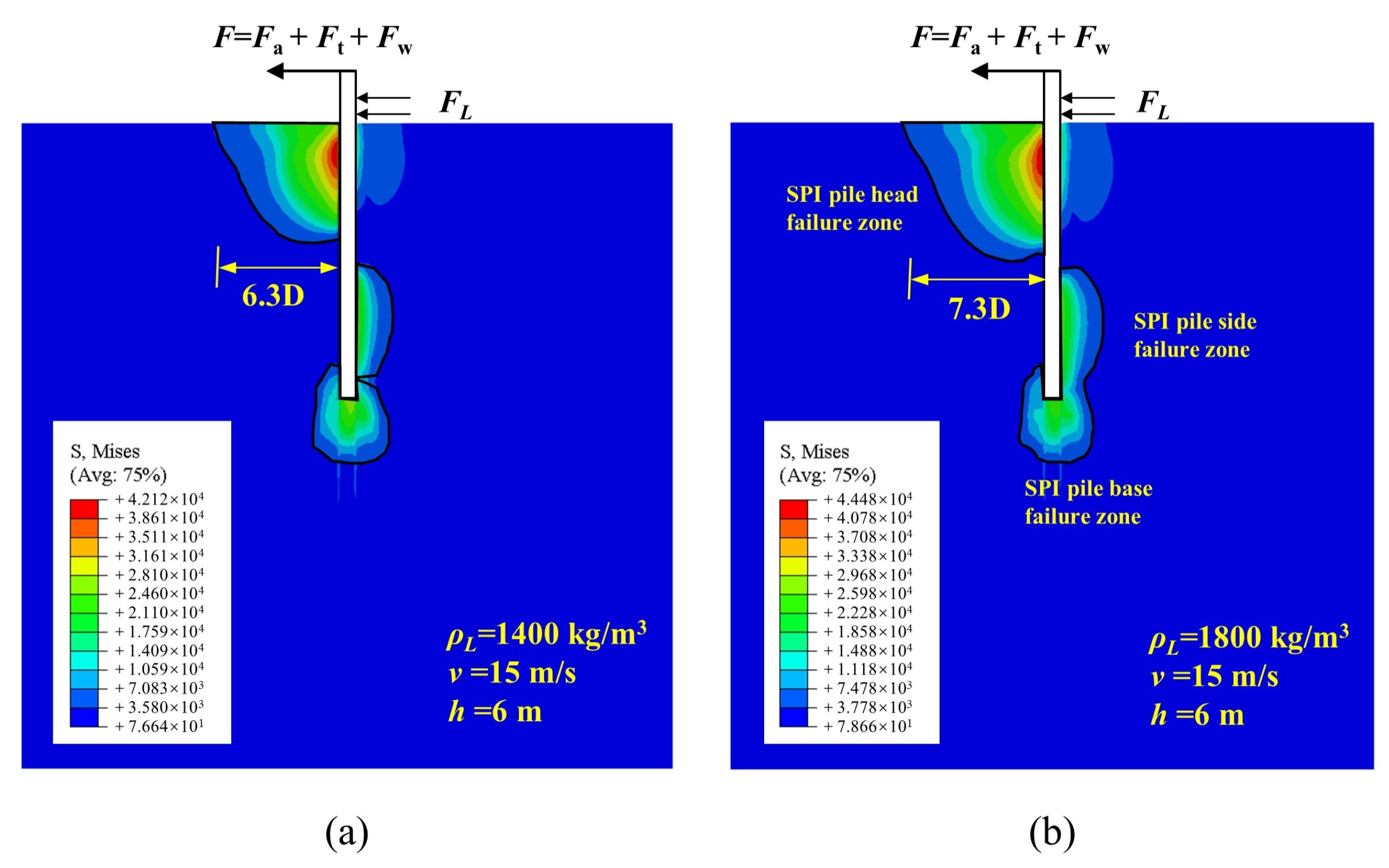
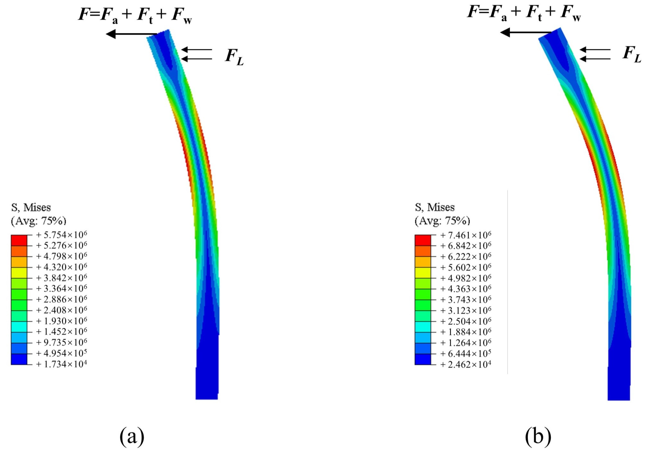
3.2.1. Effect of Submarine Landslide Density

To assess the effect of different landslide densities on monopile stability, a landslide velocity of 15 m/s and a landslide impact height of 6 m are standardized for comparison. The displacement, rotation angle, and bending moment of the monopile under various densities are depicted in Figure 6. When the landslide density is 1400 kg/m³, the resulting landslide impact force is 3,561,713 N, leading to a horizontal displacement of 0.09 m at the pile head. As the density of the seabed landslide increases to 1800 kg/m³, the landslide impact force increases to 4,574,803 N, and the pile head horizontal displacement reaches 0.13 m. Obviously, the greater the density of submarine landslides, the greater the pile head horizontal displacement. However, the gradient of the horizontal displacement at the pile head remains basically unchanged with the increase in landslide density. For every 200 kg/m³ increase in landslide density, the horizontal displacement of the pile head increases by 0.02 m. Similarly, the rate of increase in the pile rotation angle remains relatively constant with increasing landslide density. For every 200 kg/m³ increase in landslide density, the maximum pile rotation angle increases by approximately 0.04°. At a landslide density of 1400 kg/m³, the maximum rotation angle at the mudline of the pile is 0.19°, whereas it increases to 0.27° at a density of 1800 kg/m³, indicating a state of failure. The maximum bending moment of the pile increases as the landslide density increases. At a density of 1600 kg/m³, the maximum bending moment of the pile is 47.5 MN·m, which is 3.6 times the calculated result without landslide load. Meanwhile, at a density of 1800 kg/m³, the maximum bending moment of the pile reaches 61.9 MN·m, which is 4.7 times the calculated result without landslide load. To analyze the stress states of the sediment and monopile under loading, the next section primarily focuses on the Mises stress nephograms of the sediment and monopile. The aforementioned results can be elucidated by comparing the Mises stress nephograms of the sediment (Figure 7) and the monopile (Figure 8) at densities of 1400 kg/m³ and 1800 kg/m³. When the monopile is subjected to lateral loads, the sediment experiences higher compressive stress on the pressure side due to lateral loads. With the increase in density, the lateral load intensifies, resulting in increased stress in the sediment. It can be observed that the variation in landslide density does not alter the distribution of the sediment–pile interaction (SPI) failure zones. The SPI failure zones mainly include the compression failure zone occurring at the pile head, the shear failure zone caused by pile rotation at the pile base, and the lateral failure zone of the pile. The range of the SPI pile head failure zone is 6.3 D when the density is 1400 kg/m³, while that is 7.3 D when the density is 1800 kg/m³. The stress nephogram of the monopile aligns with that of the sediment, showcasing that an increase in density leads to increased stress in the monopile. The maximum stress of the monopile occurs at a depth of about 10 m below the seabed surface, which is consistent with the location of the maximum bending moment of the monopile, and it increases with the increasing displacement at the pile head.

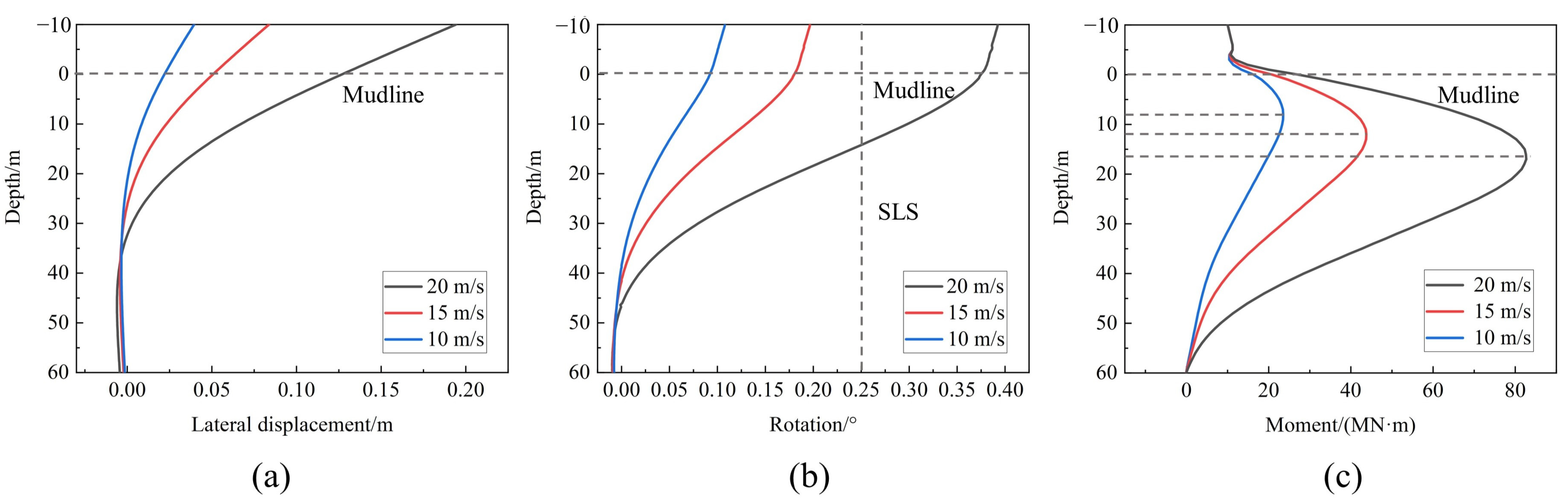
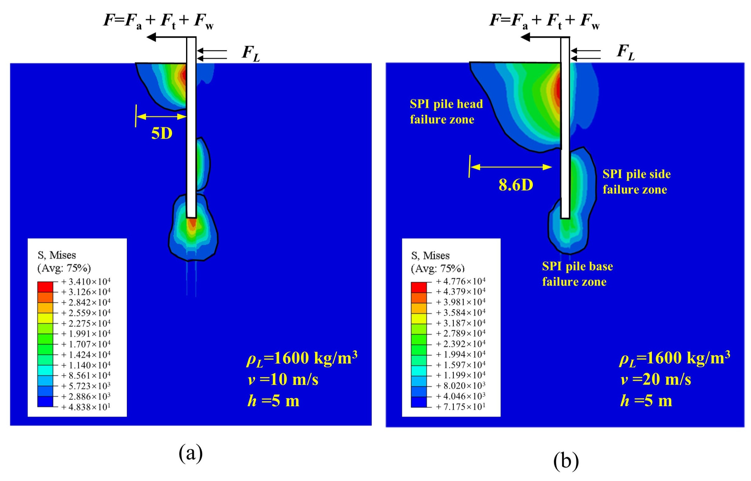
3.2.2. Effect of Submarine Landslide Velocity

The effects of different landslide velocities (10 m/s, 15 m/s, and 20 m/s) on monopile stability are analyzed, where the landslide density is 1600 kg/m³ and the impact height is 5 m. Figure 9 illustrates the horizontal displacement response of the monopile under various submarine landslide velocities. It is evident that, at a landslide velocity of 10 m/s, the resulting landslide impact force is 1,511,617 N, causing a horizontal displacement of 0.04 m at the pile head. At 15 m/s, the impact force increases to 3,390,260 N, with a pile head horizontal displacement of 0.08 m. At 20 m/s, the impact force peaks at 6,017,307 N, with a corresponding pile head horizontal displacement of 0.19 m. Clearly, higher submarine landslide velocities lead to increased impact force and pile head horizontal displacement. Furthermore, the gradient of increase in pile head horizontal displacement is more pronounced when the landslide velocity increases from 15 m/s to 20 m/s than when it increases from 10 m/s to 15 m/s, indicating a nonlinear increase in underwater landslide impact force and a steeper gradient of increase in pile head horizontal displacement with increasing landslide velocity. Moreover, greater submarine landslide velocities result in larger pile rotation angles. At 10 m/s, the maximum pile rotation angle is only 0.09°, whereas, at 20 m/s, it can reach 0.38°, indicating monopile instability. Similarly, the gradient of increase in pile rotation angle also rises gradually with increasing landslide velocity. In addition, the maximum bending moment of the pile increases with increasing landslide velocity. At 10 m/s, it is 23.5 MN·m, which is 1.8 times the calculated result without landslide load. At 20 m/s, it can reach 82.7 MN·m, which is 6.2 times the result without landslide load. The gradient of increase in maximum bending moment of the pile also gradually grows with increasing landslide velocity. It is noteworthy that the position of the inflection point of the pile bending moment shifts downward as the incidental impact load reaches a certain threshold at larger submarine landslide velocities. Figure 10 and Figure 11 depict the Mises stress nephograms of the sediment and pile body at velocities of 10 m/s and 20 m/s, respectively. It is observed that, with increasing landslide velocity, the impact force of submarine landslides increases, resulting in a significant increase in sediment stress. As a result, the area of the SPI failure zone at the pile head increases, with the horizontal range expanding from 5 D to 8.6 D. Additionally, the SPI failure zones at the pile base and pile side are interconnected. Stress gradually extends downward, and the stress concentration point moves accordingly. The distribution of stress in the monopile body corresponds to the stress distribution in the sediment. At 10 m/s, the maximum stress point is 9 m below the seabed surface, and, at 20 m/s, it is 16 m below the seabed surface. As the landslide velocity increases, the underwater landslide impact force grows, the upper monopile displacement increases, and the maximum pile body stress rises, but the stress at the pile head decreases.

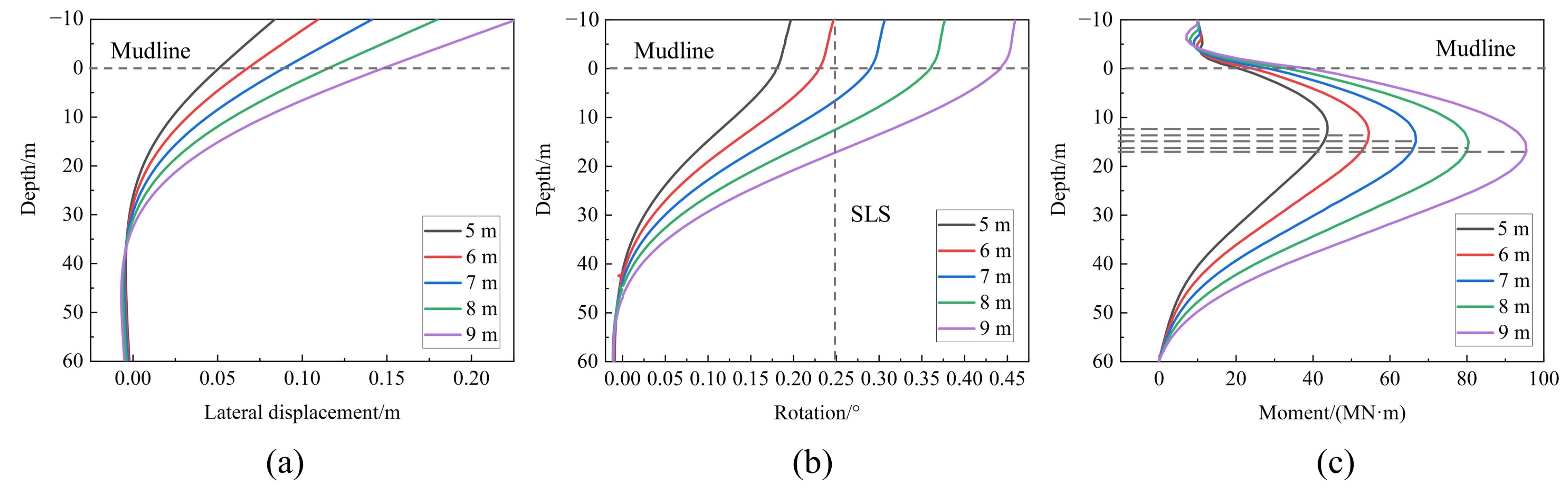
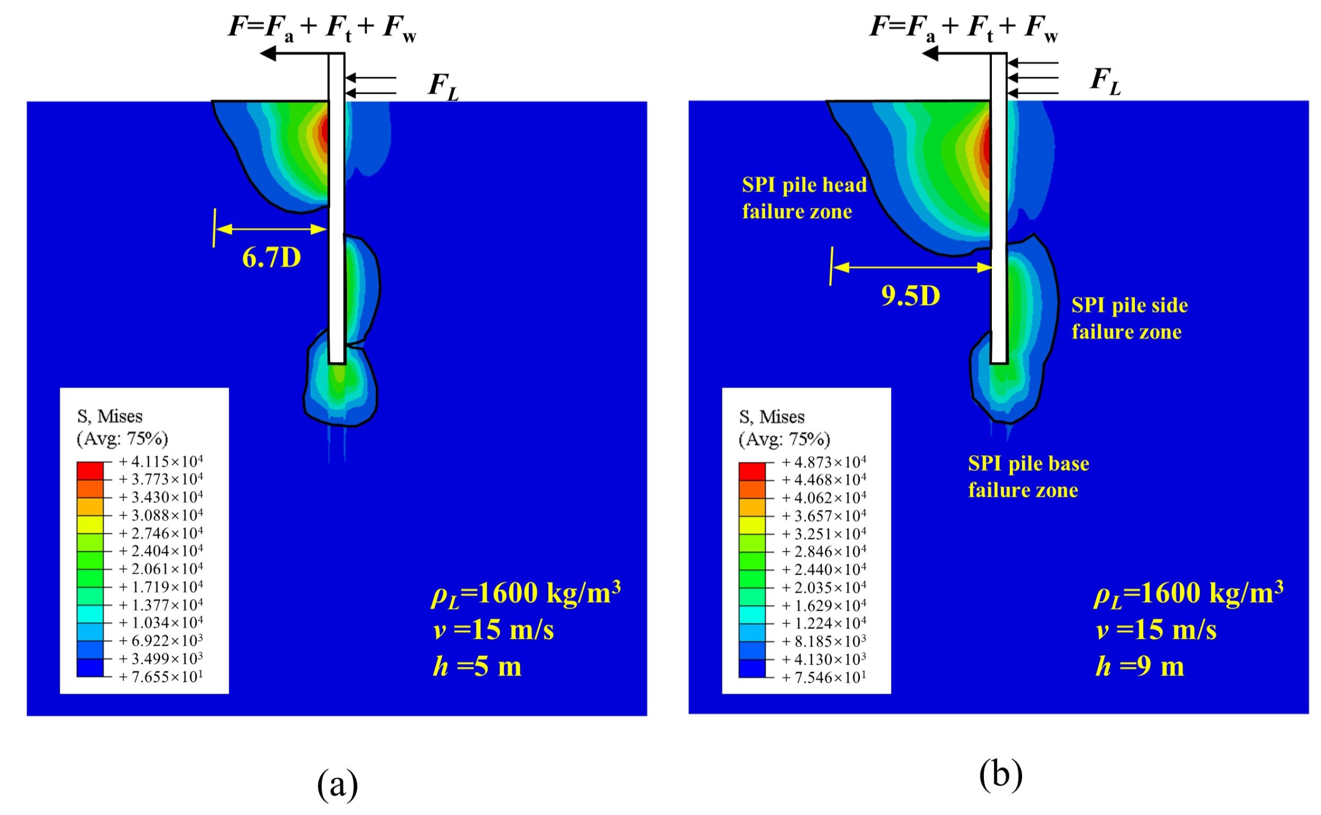
3.2.3. Effect of Submarine Landslide Impact Height

This section explores the influence of impact heights varying from 5 m to 9 m on monopile stability, where the landslide velocity is 15 m/s and the density is 1600 kg/m³. Figure 12 depicts the horizontal displacement response of a monopile under varying submarine landslide impact heights. At 5 m impact height, the landslide exerts a force of 3,390,260 N, resulting in a horizontal displacement of 0.08 m at the pile head. Conversely, at 9 m impact height, the force increases to 6,102,468 N, causing a displacement of 0.23 m. It is clear that higher impact heights yield greater forces and larger displacements. Moreover, as the submarine landslide impact heights increase, the rotation angle of the pile body also increases. The maximum rotation angle at 5 m impact height is 0.2°, while that at 9 m impact height is 0.46°, indicating instability and eventual failure of the pile. The gradient of rotation angle increases gradually with impact height, but is less significant compared with the influence of landslide velocity. For every 1 m increase in impact height, horizontal displacement at the pile head increases by approximately 0.05° to 0.07°. Likewise, changes in the maximum bending moment of the pile body follow a distinct trend. At 5 m impact height, it is 43.8 MN·m, which is 3.3 times the calculated result without considering landslide loads. Yet, at 9 m impact height, it reaches 95.5 MN·m, which is 7.2 times the calculated result. The maximum bending moment increases gradually with impact height, and it increases by 23 MN·m from 5 m to 7 m, and by 28.7 MN·m from 7 m to 9 m. Furthermore, the submarine landslide impact height affects the location of the inflection point of the bending moment of pile body. As the impact height increases, the inflection point shifts downward due to the increase in impact force and range. Figure 13 illustrates the sediment stress nephograms under different impact heights. The SPI failure zones under different landslide impact heights still distribute near the pile head, lower part of the pile side, and near the pile base. With the increase in landslide impact height, the evolutions of SPI failure zones at pile head and pile base exhibit opposite trends. The range of the SPI failure zone at the pile head gradually increases from 6.7 D to 9.5 D, while the range of the SPI failure zone at the pile base gradually decreases. This reflects an increased contribution of the upper soil to the resistance force as the landslide impact height increases. Figure 14 displays the distribution of the pile body stress. With increasing landslide impact height, stress increases, and the maximum stress point shifts downward, corresponding to the change in pile bending moment.

3.3. The Influence of Seabed Sediment Strength on the Stability of Monopiles

This section investigates the influence of seabed sediment strength on monopile stability. Wang and Yu [51] conducted laboratory direct shear tests to evaluate the strength of marine sediments. Based on the test results, this study selects sediment cohesion values of 5 kPa, 10 kPa, 15 kPa, and 20 kPa, along with internal friction angles of 0°, 5°, 10°, and 15° for comparative analysis. The loading conditions on the monopile remain the same as before, with a landslide velocity of 15 m/s, a landslide density of 1600 kg/m³, a landslide impact height of 7 m, and a landslide impact force of 4,746,364 N.

3.3.1. Effect of Cohesion

Figure 15 depicts the displacement and rotation at the mudline of a monopile under varying sediment cohesion, where the internal friction angle is 10°. As sediment cohesion diminishes, both horizontal displacement and rotation increase. For instance, the mudline displacement at 20 kPa cohesion is only 0.049 m with a rotation angle of 0.19°. Conversely, the mudline displacement at 5 kPa cohesion increases to 0.23 m, accompanied by a rotation angle of 0.50°, indicating instability. Notably, the decrease in sediment cohesion yields more significant increases in both the displacement and rotation at the mudline. A decrease in cohesion from 10 kPa to 5 kPa results in a displacement change of 0.13 m and a rotation angle increase of 0.22°, which implies that the horizontal load-bearing capacity of the sediment on a monopile is lost when cohesion falls below 10 kPa. Fitting a hyperbolic curve to monopile displacement and rotation for various sediment cohesion levels can yield empirical formulas correlating sediment cohesion to monopile behavior. Comparative analysis of Mises stress contour plots of sediment (Figure 16) and monopile stress distribution (Figure 17) at cohesion values of 20 kPa and 5 kPa demonstrates that, as sediment cohesion decreases, both the SPI failure zones at the pile head and pile base undergo substantial expansion due to the increased horizontal displacement of the monopile. Specifically, the horizontal span of the SPI pile head failure zone escalates from 5.9 D to 13.8 D. Meanwhile, there is a significant reduction in maximum stress, which plummets from 71.95 kPa to 28.17 kPa. This observation suggests a more pronounced dispersion of stress under these conditions. In addition, as cohesion decreases, stress concentration points shift downward, which transitions monopile damage from horizontal to depth-wise, corresponding to stress changes in the monopile with the sediment. The reduction in cohesion diminishes the load-bearing capacity of the sediment, resulting in overall tilting of the monopile.

3.3.2. Effect of Internal Friction Angle

Figure 18 illustrates the displacement and rotation angle at the mudline of the monopile for different internal friction angles under 10 kPa cohesion. It can be observed that, as the internal friction angle decreases, the horizontal displacement and rotation angle of the monopile increase. When the internal friction angle is 15°, the pile displacement is 0.076 m and the rotation angle is 0.25°, indicating instability of the monopile. When the internal friction angle decreases to 0°, the pile displacement increases to 0.147 m and the rotation angle increases to 0.38°. It is observed that a decrease in the internal friction angle leads to a slightly larger increase in displacement and rotation angle at the mudline of the monopile. Empirical formulas relating the sediment internal friction angle to pile displacement and the rotation angle can be obtained by linearly fitting the displacement and rotation angle of the monopile at the mudline for different internal friction angles. Figure 19 and Figure 20 show the Mises stress nephograms of sediment and the pile body when the internal friction angles are 15° and 0°, respectively. It can be observed that, when the internal friction angle decreases, the areas of both the SPI pile head failure zone and the SPI pile base influence zone significantly increase. The influence zone at the pile head increases from 6.6 D to 13.6 D and the maximum stress decreases from 62.61 kPa to 19.82 kPa. When the internal friction angle is 15°, the stress concentration zone is located on the compression side of the sediment, which is approximately 10–15 m below the seabed surface, whereas, when the internal friction angle is 0°, the stress concentration zone significantly expands. The sediment from the seabed surface to a depth of 35 m below the seabed surface undergoes compression due to the displacement of the monopile, resulting in stress concentration on the compression side. Meanwhile, when the internal friction angle is 0°, significant stress concentration also occurs at the pile base, indicating that, in this case, the impact of the landslide on the monopile base cannot be ignored in design. As the internal friction angle decreases, the stress on the pile body gradually increases, and the stress concentration zone of the pile body gradually shifts downward. However, the monopile does not undergo significant tilting, indicating that the change in the internal friction angle has a relatively small effect on pile displacement.

4. Conclusions

This study quantifies the wind, wave, current loads, and seabed landslide loads acting on offshore wind turbine structures during their service life, and simplifies them into horizontal loads and moments applied to the pile head. A finite element analysis model of offshore wind turbine foundation under complex lateral loading conditions is established, and the stability of monopiles under the coupling effect of seabed landslides as well as offshore wind and wave loads is investigated.

• As the density, velocity, and impact height of submarine landslides increase, the force on the monopile increases. Consequently, all the horizontal displacement, pile rotation angle, and maximum bending moment at the pile head increase. The escalation in submarine landslide density and impact height yields a proportional increase in the horizontal displacement, pile rotation angle, and maximum bending moment. Moreover, an increase in submarine landslide velocity leads to a hyperbolic surge in the horizontal displacement, pile rotation angle, and maximum bending moment. Once a specific lateral loading threshold is reached, three distinct SPI failure zones emerge within the seabed sediment, i.e., the compressive wedge failure zone at the pile head, the rotational shear failure zone at the pile base, and the failure zone along the pile side. Further increase in lateral loading prompts a gradual expansion of the sediment compression failure zone at the pile head, while the shear failure zone at the pile base progressively intertwines with the failure zone along the pile side. In the scenario of the designated case study, the cumulative rotation angle at the mudline of the monopile reaches 0.27° when the horizontal influence range at the pile head extends to 7.3 D, thereby triggering instability failure in accordance with DNV standards.
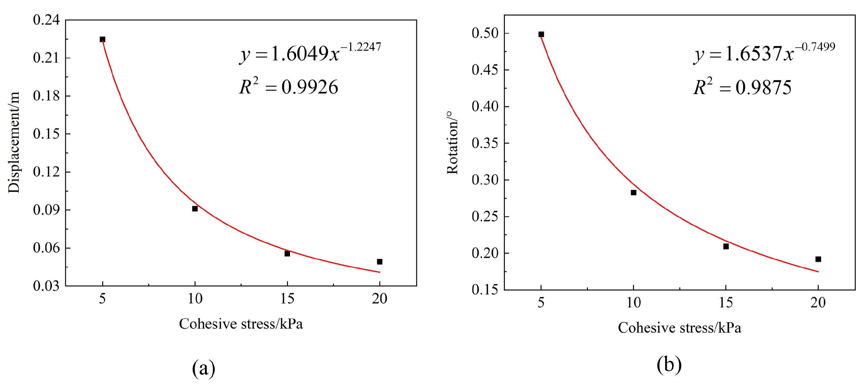
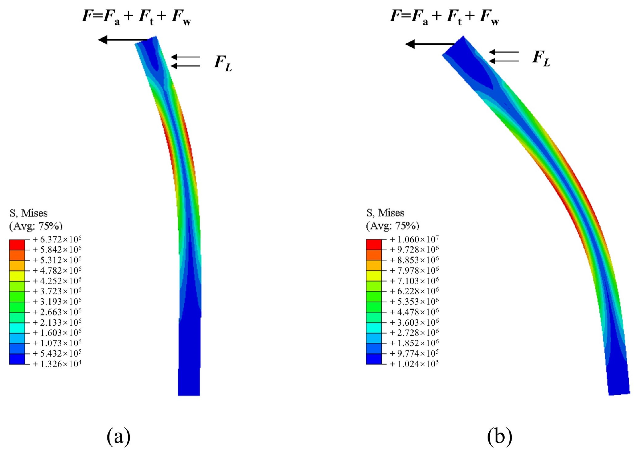
• A decrease in the cohesion of the seabed sediment subjected to the same lateral load leads to a reduction of the horizontal bearing capacity of the sediment. Consequently, this triggers a hyperbolic increase in displacement and rotation angle at the mudline of the monopile. For instance, when the cohesion of the seabed sediment decreases from 20 kPa to 5 kPa, the area of sediment compression failure zone at the pile head enlarges and the horizontal influence range surges from 5.9 D to 13.8 D. It is noteworthy that the area of the full-flow failure zone on the pile side decreases, while the area of the shear failure zone at the pile base increases. The shear failure zone at the pile base extends upwards to cover the original failure zone on the pile side. In the context of the specified case study, the monopile experiences instability failure when the cohesion of the seabed sediment drops below 10 kPa.
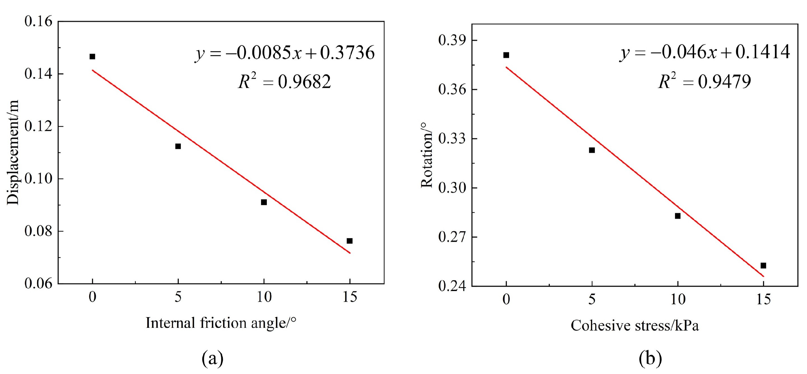
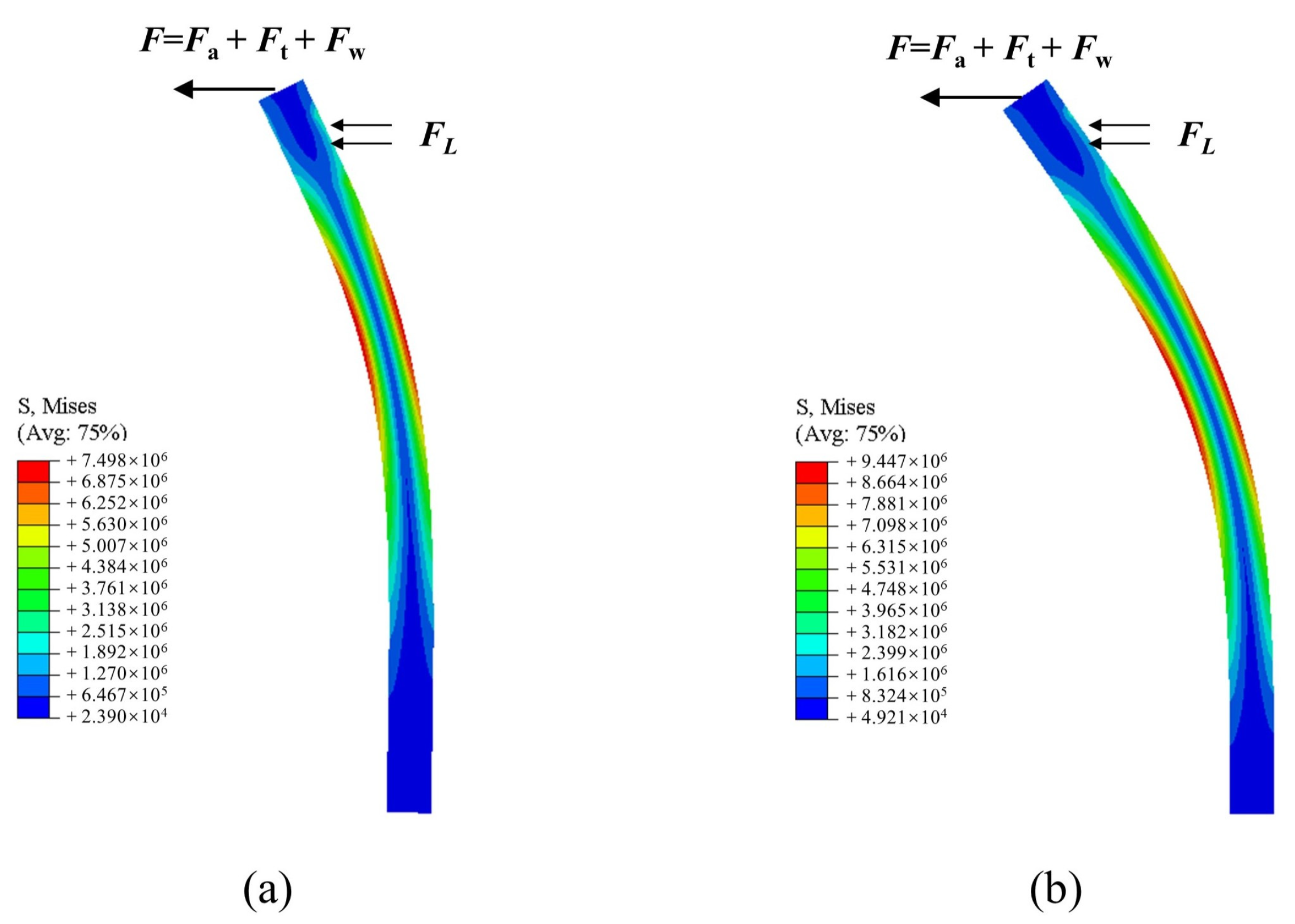
• Under the same lateral load, a decrease in the internal friction angle of the seabed sediment leads to a linear increase in displacement and rotation angle at the mudline of the monopile. When the internal friction angle decreases from 15° to 0°, the area of the sediment compression failure zone at the pile head enlarges, and the horizontal influence range expands from 6.6 D to 13.6 D. The failure zone on the pile side merges with the shear failure zone on the pile base. Concurrently, the area of stress concentration zones on the compression side of the pile head and on the opposite side of the pile base, where seabed sediments are distributed, increases significantly. This stress concentration renders sediment more susceptible to failure. In the conditions of the chosen case study, the monopile experiences instability failure when the internal friction angle of the sediment is below 15°.
• This study investigates the stability of wind turbine foundations during operation by simplifying submarine landslide, wind, wave, and current loads into horizontal loads, which offers insights into the design of such foundations. However, further research should consider the distribution and instantaneous dynamic characteristics of submarine landslide, wind, wave, and flow loads, and conduct more comprehensive calculations to enhance analytical precision. In addition, future studies can integrate analysis with field-measured environmental data to better quantify environmental loads.

References

1. Esteban, M.D.; Diez, J.J.; López, J.S.; Negro, V. Why offshore wind energy? Renew. Energy 2011, 36, 444–450. [Google Scholar] [CrossRef]
2. Zhang, J.H.; Hao, W. Development of offshore wind power and foundation technology for offshore wind turbines in China. Ocean Eng. 2022, 266, 113256. [Google Scholar] [CrossRef]
3. Soares-Ramos, E.P.P.; De Oliveira-Assis, L.; Sarrias-Mena, R.; Fernández-Ramírez, L.M. Current status and future trends of offshore wind power in Europe. Energy 2020, 202, 117787. [Google Scholar] [CrossRef]
4. Simoncelli, M.; Zucca, M.; Ghilardi, M. Structural health monitoring of an onshore steel wind turbine. J. Civ. Struct. Health Monit. 2024, 1–15. [Google Scholar] [CrossRef]
5. Global Wind Energy Council. Global offshore Wind Report 2023. Available online: https://gwec.net/gwecs-global-offshore-wind-report-2023/ (accessed on 28 August 2023).
6. Xie, M.; Lopez-Querol, S. Numerical simulations of the monotonic and cyclic behaviour of offshore wind turbine monopile foundations in clayey soils. J. Mar. Sci. Eng. 2021, 9, 1036. [Google Scholar] [CrossRef]
7. Chen, Y.; Gu, M.; Chen, R.; Kong, L.; Zhang, Z.; Bian, X. Behavior of pile group with elevated cap subjected to cyclic lateral loads. China Ocean Eng. 2015, 29, 565–578. [Google Scholar] [CrossRef]
8. Zeng, X.; Shi, W.; Michailides, C.; Zhang, S.; Li, X. Numerical and experimental investigation of breaking wave forces on a monopile-type offshore wind turbine. Renew. Energy 2021, 175, 501–519. [Google Scholar] [CrossRef]
9. Shi, Y.; Yao, W.; Jiang, M. Dynamic analysis on monopile supported offshore wind turbine under wave and wind load. Structures 2023, 47, 520–529. [Google Scholar] [CrossRef]
10. Miles, J.; Martin, T.; Goddard, L. Current and wave effects around windfarm monopile foundations. Coast. Eng. 2017, 121, 167–178. [Google Scholar] [CrossRef]
11. Ong, M.C.; Li, H.; Leira, B.J.; Myrhaug, D. Dynamic analysis of offshore monopile wind turbine including the effects of wind-wave loading and soil properties. In Proceedings of the International Conference on Offshore Mechanics and Arctic Engineering, Nantes, France, 9–14 June 2013; Volume 55423. [Google Scholar]
12. Buljac, A.; Kozmar, H.; Yang, W.; Kareem, A. Concurrent wind, wave and current loads on a monopile-supported offshore wind turbine. Eng. Struct. 2022, 255, 113950. [Google Scholar] [CrossRef]
13. Achmus, M.; Kuo, Y.S.; Abdel-Rahman, K. Behavior of monopile foundations under cyclic lateral load. Comput. Geotech. 2009, 36, 725–735. [Google Scholar] [CrossRef]
14. Wu, T.; Lu, Z.; Dou, D. Model Tests and Finite Element Analysis of Behaviors of Ocean and Offshore Elevated Piles under Lateral Load. Sci. Technol. Eng. 2013, 13, 7697–7702. (In Chinese) [Google Scholar]
15. Guo, X.; Liu, X.; Li, M.; Lu, Y. Lateral force on buried pipelines caused by seabed slides using a CFD method with a shear interface weakening model. Ocean. Eng. 2023, 280, 114663. [Google Scholar] [CrossRef]
16. Rafiei, A.; Rahman, M.S.; Gabr, M.A.; Ghayoomi, M. Analysis of wave-induced submarine landslides in nearly saturated sediments at intermediate water depths. Mar. Georesources Geotechnol. 2022, 40, 1411–1423. [Google Scholar] [CrossRef]
17. Liu, X.; Wang, Y.; Zhang, H.; Guo, X. Susceptibility of typical marine geological disasters: An overview. Geoenvironmental. Disasters 2023, 10, 10. [Google Scholar] [CrossRef]
18. Guo, X.; Fan, N.; Liu, Y.; Liu, X.; Wang, Z.; Xie, X.; Jia, Y. Deep seabed mining: Frontiers in engineering geology and environment. Int. J. Coal Sci. Technol. 2023, 10, 23. [Google Scholar] [CrossRef]
19. Guo, X.; Liu, X.; Zheng, T.; Zhang, H.; Lu, Y.; Li, T. A mass transfer-based LES modelling methodology for analyzing the movement of submarine sediment flows with extensive shear behavior. Coast. Eng. 2024, 191, 104531. [Google Scholar] [CrossRef]
20. Guo, X.; Fan, N.; Zheng, D.; Fu, C.; Wu, H.; Zhang, Y.; Song, X.; Nian, T. Predicting impact forces on pipelines from deep-sea fluidized slides: A comprehensive review of key factors. Int. J. Min. Sci. Technol. 2024, 34, 211–225. [Google Scholar] [CrossRef]
21. Wang, Z.; Zheng, D.; Guo, X.; Gu, Z.; Shen, Y.; Nian, T. Investigation of offshore landslides impact on bucket foundations using a coupled SPH–FEM method. Geoenvironmental. Disasters 2024, 11, 2. [Google Scholar] [CrossRef]
22. Guo, X.; Stoesser, T.; Zheng, D.; Luo, Q.; Liu, X.; Nian, T. A methodology to predict the run-out distance of submarine landslides. Comput. Geotech. 2023, 153, 105073. [Google Scholar] [CrossRef]
23. Mohrig, D.; Ellis, C.; Parker, G.; Kelin, X.; Midhat, H. Hydroplaning of subaqueous debris flows. Geol. Soc. Am. Bull. 1998, 110, 387–394. [Google Scholar] [CrossRef]
24. Guo, X.; Nian, T.; Stoesser, T. Using dimpled-pipe surface to reduce submarine landslide impact forces on pipelines at different span heights. Ocean. Eng. 2022, 244, 110343. [Google Scholar] [CrossRef]
25. De Blasio, F.V.; Elverhøi, A.; Issler, D.; Harbitz, C.B.; Bryn, P.; Lien, R. Flow models of natural debris flows originating from overconsolidated clay materials. Mar. Geol. 2004, 213, 439–455. [Google Scholar] [CrossRef]
26. Hsu, S.K.; Kuo, J.; Chung-Liang, L.; Ching-Hui, T.; Doo, W.B.; Ku, C.Y.; Sibuet, J.C. Turbidity currents, submarine landslides and the 2006 Pingtung earthquake off SW Taiwan. TAO Terr. Atmos. Ocean. Sci. 2008, 19, 7. [Google Scholar] [CrossRef]
27. Li, D.L.; Yan, E.C.; Feng, B. Impact of submarine debris flow on offshore piles. J. Zhejiang Univ. Eng. Sci. 2019, 53, 2342–2347. (In Chinese) [Google Scholar]
28. Li, R.Y.; Chen, J.J.; Liao, C.C. Numerical study on interaction between submarine landslides and a monopile using CFD techniques. J. Mar. Sci. Eng. 2021, 9, 736. [Google Scholar] [CrossRef]
29. Xi, R.; Du, X.; Wang, P.; Xu, C.; Zhai, E.; Wang, S. Dynamic analysis of 10 MW monopile supported offshore wind turbine based on fully coupled model. Ocean. Eng. 2021, 234, 109346. [Google Scholar] [CrossRef]
30. Bisoi, S.; Haldar, S. Dynamic analysis of offshore wind turbine in clay considering soil–monopile–tower interaction. Soil Dyn. Earthq. Eng. 2014, 63, 19–35. [Google Scholar] [CrossRef]
31. Arany, L.; Bhattacharya, S.; Macdonald, J.; Hogan, S.J. Design of monopiles for offshore wind turbines in 10 steps. Soil Dyn. Earthq. Eng. 2017, 92, 126–152. [Google Scholar] [CrossRef]
32. Frohboese, P.; Schmuck, C.; Hassan, G.G. Thrust coefficients used for estimation of wake effects for fatigue load calculation. In Proceedings of the European Wind Energy Conference, Berlin, Germany, 23–24 November 2010; pp. 1–10. [Google Scholar]
33. Charlton, T.S.; Rouainia, M. Geotechnical fragility analysis of monopile foundations for offshore wind turbines in extreme storms. Renew. Energy 2022, 182, 1126–1140. [Google Scholar] [CrossRef]
34. JTG/T 3360-01—2018; Recommend Profession Standard of the People’s Republic of China, Code for Wind Resistance Design of Highway Bridges. People’s Communications Press: Beijing, China, 2016. Available online: https://xxgk.mot.gov.cn/2020/jigou/glj/202006/t20200623_3313096.html (accessed on 1 March 2019).
35. NB/T 10105-2018; Energy Industry Recommended Standard of the People’s Republic of China, Code for Basic Design of Wind Turbines for Offshore Wind Farm Projects. China Water Power Press: Beijing, China, 2018. Available online: https://www.chinesestandard.net/PDF/English.aspx/NBT10105-2018 (accessed on 25 December 2018).
36. Morison, J.R.; Johnson, J.W.; Schaaf, S.A. The force exerted by surface waves on piles. J. Pet. Technol. 1950, 2, 149–154. [Google Scholar] [CrossRef]
37. JTS 145-2015; Profession Standard of the People’s Republic of China, Code of Hydrology for Harbour. China Communications Press: Beijing, China, 1998; pp. 77–78. Available online: https://xxgk.mot.gov.cn/2020/jigou/syj/202006/t20200623_3313586.html (accessed on 31 August 2015).
38. Zhang, C.; Tang, G.; Lu, L.; Jin, Y.; An, H.; Cheng, L. Flow-induced vibration of two tandem square cylinders at low Reynolds number: Transitions among vortex-induced vibration, biased oscillation and galloping. J. Fluid Mech. 2024, 986, A10. [Google Scholar] [CrossRef]
39. Feng, B.; Sun, H.L.; Cai, Y.Q. Experimental study of submarine landslide impact on offshore wind power piles. Ocean. Eng. 2019, 37, 114–121. (In Chinese) [Google Scholar]
40. Herschel, W.H.; Bulkley, R. Konsistenzmessungen von gummi-benzollösungen. Kolloid-Zeitschrift 1926, 39, 291–300. [Google Scholar] [CrossRef]
41. Reese, L.C.; van Impe, W. Derivation of equations and methods of solution. In Book Single Piles and Pile Groups under Lateral Loading, 2nd ed.; Taylor and Francis: Abingdon, UK, 2001; pp. 23–24. [Google Scholar]
42. Abbas, J.M.; Chik, Z.H.; Taha, M.R. Single pile simulation and analysis subjected to lateral load. Electron. J. Geotech. Eng. 2008, 13, 1–15. [Google Scholar]
43. Johnson, K.; Lemcke, P.; Karunasena, W.; Sivakugan, N. Modelling the load–deformation response of deep foundation under oblique loading. Environ. Model. Softw. 2006, 21, 1375–1380. [Google Scholar] [CrossRef]
44. Hu, Q.; Han, F.; Prezzi, M.; Salgado, R.; Zhao, M. Lateral load response of large-diameter monopiles in sand. Géotechnique 2022, 72, 1035–1050. [Google Scholar] [CrossRef]
45. Liu, H.J.; Sun, P.P.; Geng, H.R.; Hao, R. Horizontal bearing capacity of offshore wind power pile foundation under different sea conditions and geological conditions. Period. Ocean. Univ. China 2019, 8, 51–58. (In Chinese) [Google Scholar]
46. Dai, S.; Han, B.; Wang, B.; Luo, J.; He, B. Influence of soil scour on lateral behavior of large-diameter offshore wind-turbine monopile and corresponding scour monitoring method. Ocean. Eng. 2021, 239, 109809. [Google Scholar] [CrossRef]
47. Zhang, X.L.; Liu, J.X.; Han, Y.; Du, X.L. A framework for evaluating the bearing capacity of offshore wind power foundation under complex loadings. Appl. Ocean Res. 2018, 80, 66–78. [Google Scholar] [CrossRef]
48. DNV GL, DNVGL-ST-0126 Support Structures for Wind Turbines, 2018. Edition July 2018. Available online: https://www.dnv.com/energy/standards-guidelines/dnv-st-0126-support-structures-for-wind-turbines (accessed on 1 December 2021).
49. Takahashi, T. Mechanical characteristics of debris flow. J. Hydraul. Div. 1978, 104, 1153–1169. [Google Scholar] [CrossRef]
50. Laberg, J.S.; Vorren, T.O. A late Pleistocene submarine slide on the Bear Island trough mouth fan. Geo-Mar. Lett. 1993, 13, 227–234. [Google Scholar] [CrossRef]
51. Wang, X.F.; Yu, H.G. The experience relationship between the state and the direct shear test index about marine facies clayed soil. In Proceedings of the National Engineering Geology Academic Conference and “Engineering Geology and West Coast Construction” Academic Conference, Fujian, China, 17 November 2013; Volume 5. (In Chinese). [Google Scholar]
Figure 1. Generalization of load conditions on a monopile foundation of offshore wind turbines.
Jmse 12 00915 g001
Figure 2. Schematic diagram of load simplification.
Jmse 12 00915 g002
Figure 3. Pile–soil interaction finite element model.
Jmse 12 00915 g003
Figure 4. Effect of mesh size in pile–soil contact zone on horizontal load–displacement response curves.
Jmse 12 00915 g004
Figure 5. Comparison of horizontal load–displacement curves between previous results [46] and results of this study.
Jmse 12 00915 g005
Figure 6. The effect of different landslide densities on the response of a monopile: (a) displacement of pile; (b) rotation angle of pile; (c) bending moment of pile.
Jmse 12 00915 g006
Figure 7. Stress nephograms of sediment at different submarine landslide densities: (a) the landslide density is 1400 kg/m3; (b) the landslide density is 1800 kg/m3.
Jmse 12 00915 g007
Figure 8. Stress nephograms of pile body at different submarine landslide densities (deformation coefficient of 100): (a) the landslide density is 1400 kg/m3; (b) the landslide density is 1800 kg/m3.
Jmse 12 00915 g008
Figure 9. The effect of different landslide velocities on the response of a monopile: (a) displacement of pile; (b) rotation angle of pile; (c) bending moment of pile.
Jmse 12 00915 g009
Figure 10. Stress nephograms of sediment at different submarine landslide velocities: (a) v = 10 m/s; (b) v = 20 m/s.
Jmse 12 00915 g010
Figure 11. Stress nephograms of pile body at different submarine landslide velocities (deformation coefficient of 100): (a) v = 10 m/s; (b) v = 20 m/s.
Jmse 12 00915 g011
Figure 12. The effect of different submarine landslide impact heights on the response of a monopile: (a) displacement of pile; (b) rotation angle of pile; (c) bending moment of pile.
Jmse 12 00915 g012
Figure 13. Stress nephograms of sediment at different submarine landslide impact heights: (a) h = 5 m; (b) h = 9 m.
Jmse 12 00915 g013
Figure 14. Stress nephograms of pile body at different submarine landslide impact heights (deformation coefficient of 100): (a) h = 5 m; (b) h = 9 m.
Jmse 12 00915 g014
Figure 15. Displacement and rotation at the mudline of a monopile under different cohesion: (a) displacement at the mudline; (b) rotation at the mudline.
Jmse 12 00915 g015
Figure 16. Stress nephograms of sediment under different cohesion: (a) cohesion is 20 kPa; (b) cohesion is 5 kPa.
Jmse 12 00915 g016
Figure 17. Stress nephograms of pile body under different cohesion (deformation coefficient of 100): (a) cohesion is 20 kPa; (b) cohesion is 5 kPa.
Jmse 12 00915 g017
Figure 18. Displacement and rotation at the mudline of a monopile under different internal friction angles: (a) displacement at the mudline; (b) rotation at the mudline.
Jmse 12 00915 g018
Figure 19. Stress nephograms of sediment under different internal friction angles: (a) internal friction angle is 15°; (b) internal friction angle is 0°.
Jmse 12 00915 g019
Figure 20. Stress nephograms of pile body under different internal friction angles (deformation coefficient of 100): (a) internal friction angle is 15°; (b) internal friction angle is 0°.
Jmse 12 00915 g020