A Method for Full-Depth Sound Speed Profile Reconstruction Based on Average Sound Speed Extrapolation

Abstract
1. Introduction
2. Methods
2.1. The Principle of EOF
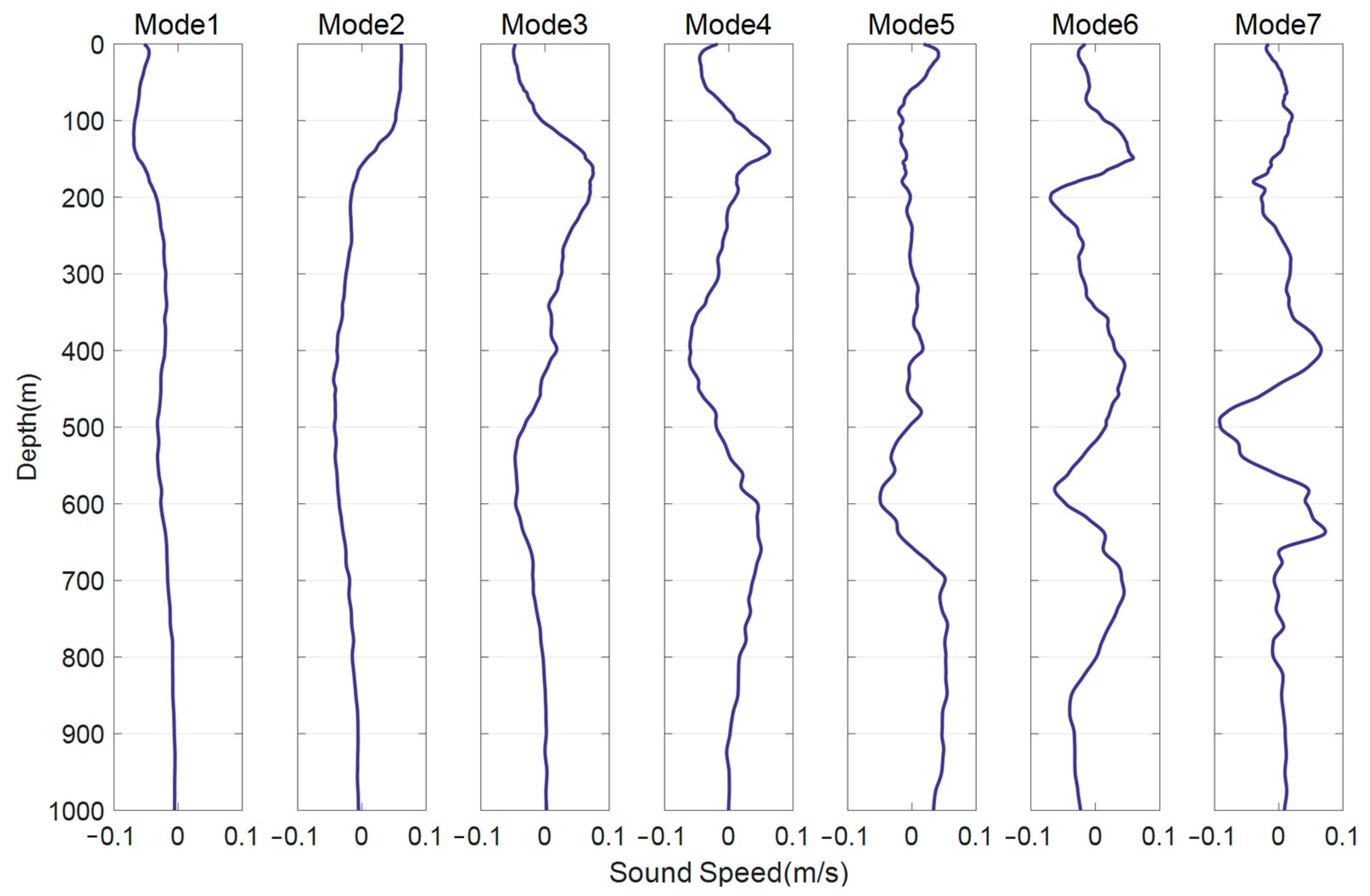
2.1.1. EOF Decomposition and Reconstruction of Sound Speed Profiles
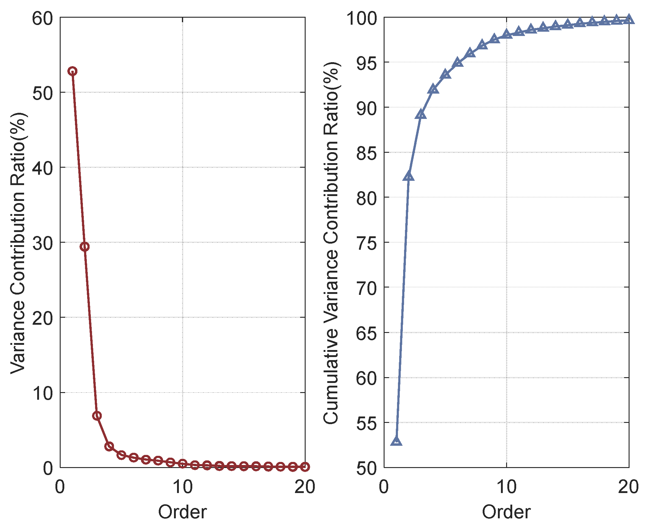
2.1.2. Variance Contribution Ratio of Spatial Modes
2.2. Method 1
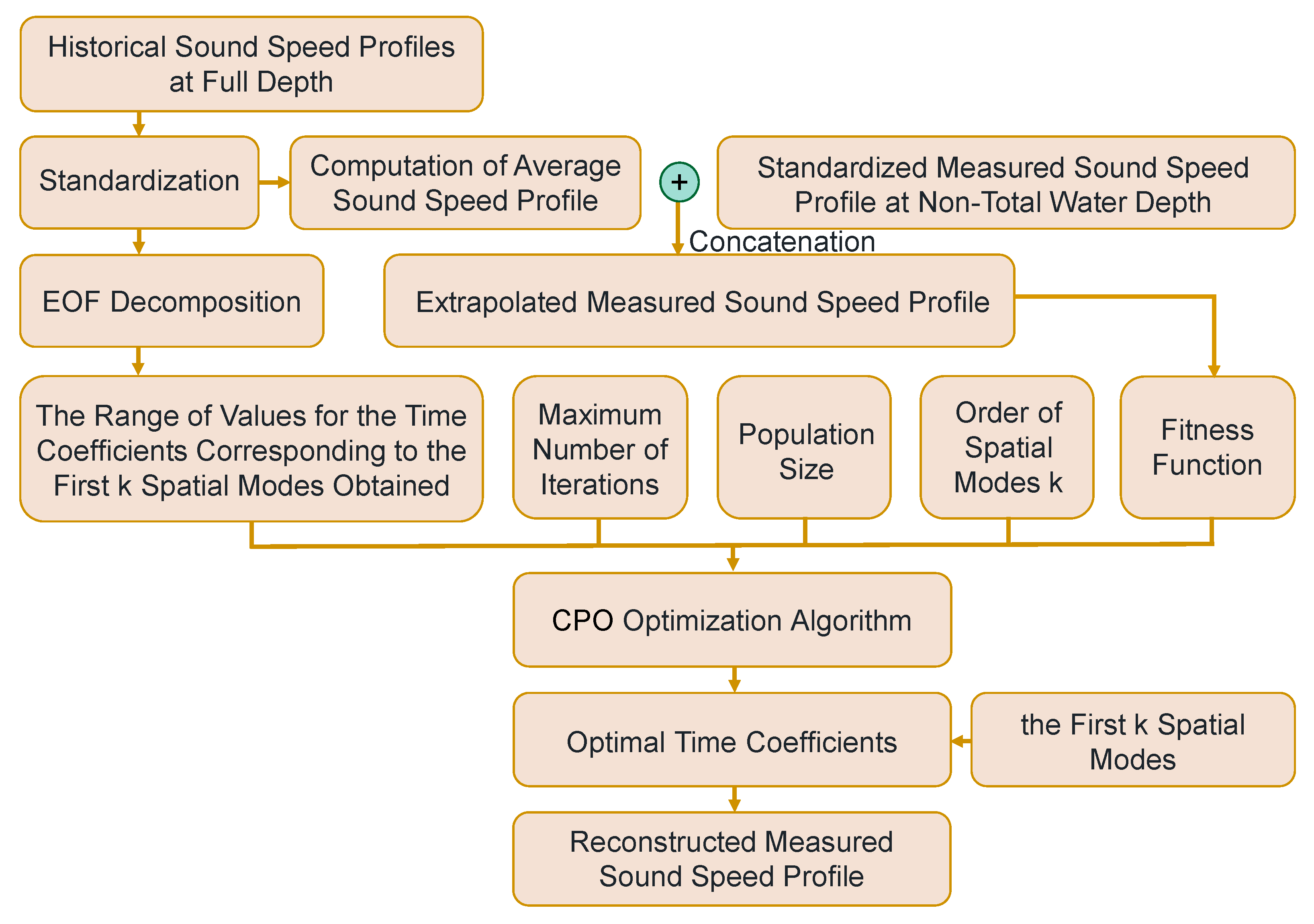
2.3. Method 2
2.3.1. CPO
2.3.2. Basic Process
3. Materials and Experiments
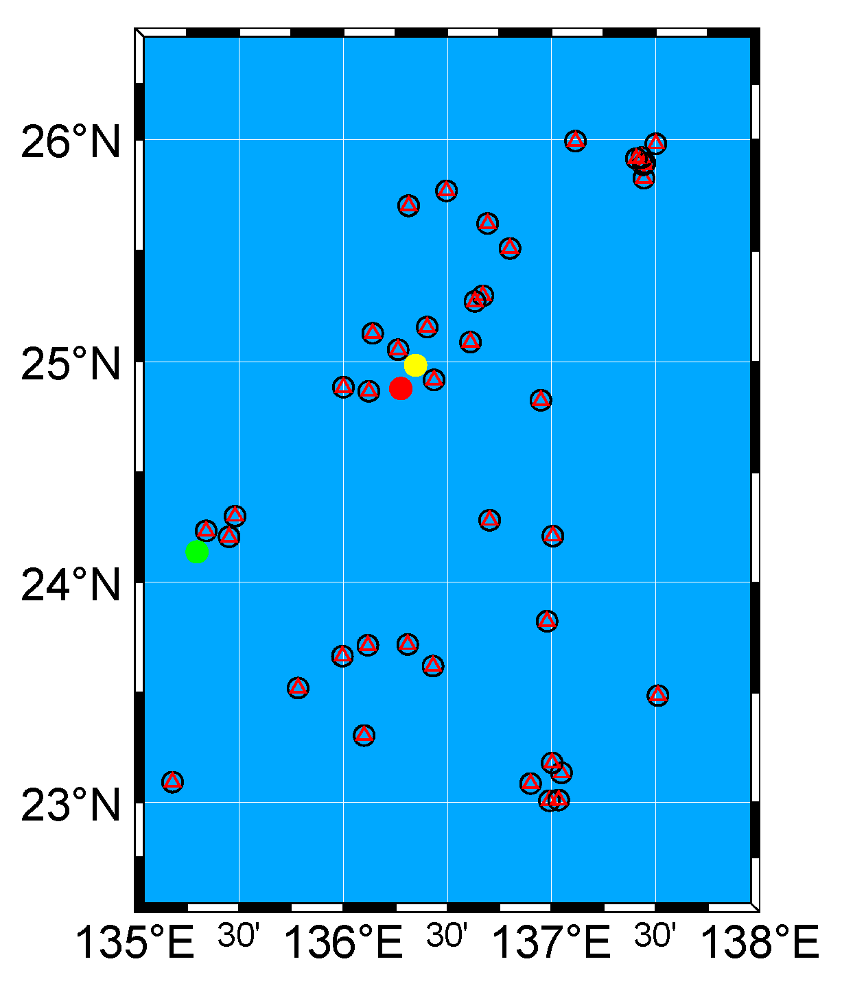
3.1. Experimental Data
3.2. Experimental Process
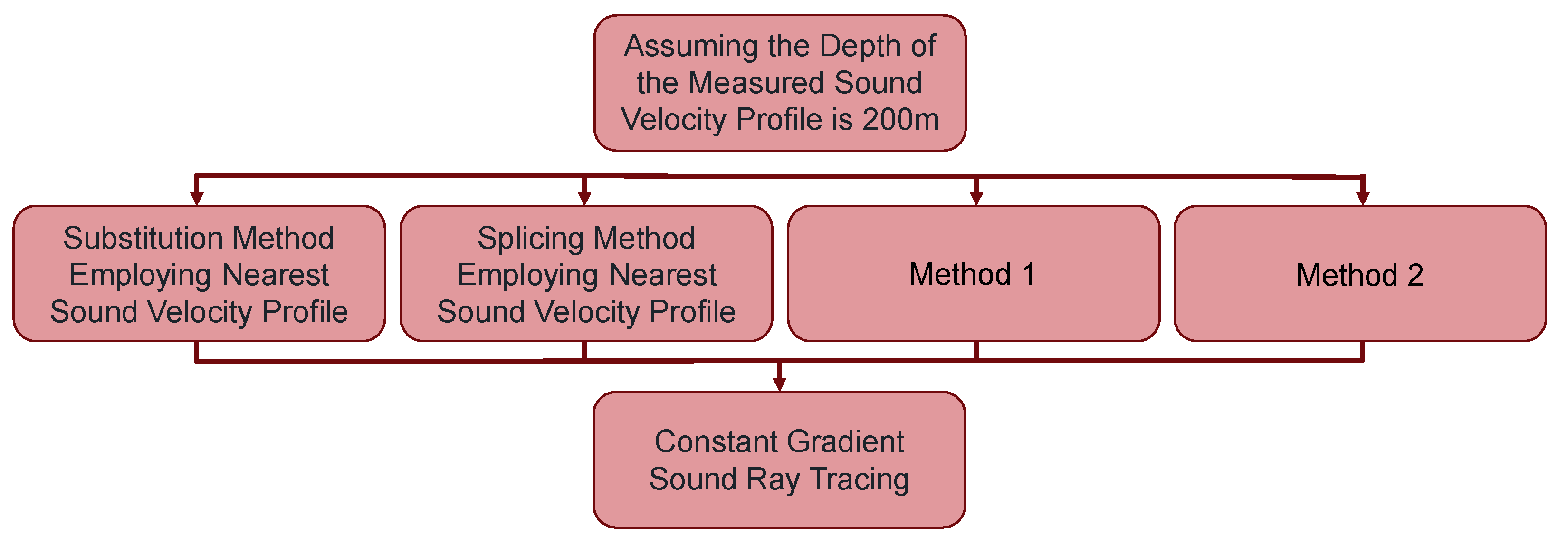
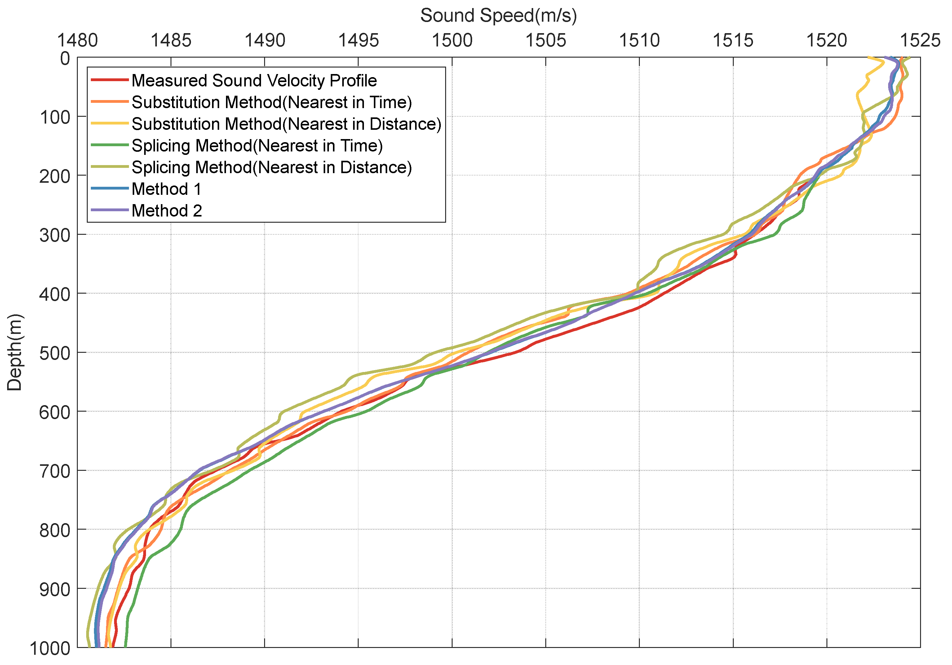
3.2.1. Reconstruction of the Measured Sound Speed Profile Using Four Methods
- Method 1
- 2.
- Method 2
3.2.2. Constant Gradient Sound Ray Tracing and Accuracy Evaluation
3.3. Evaluation Metrics
4. Results and Discussion
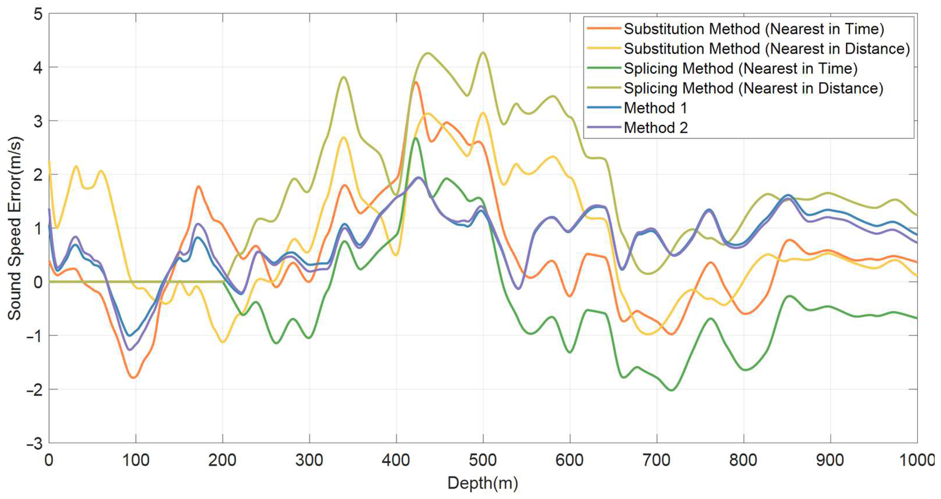
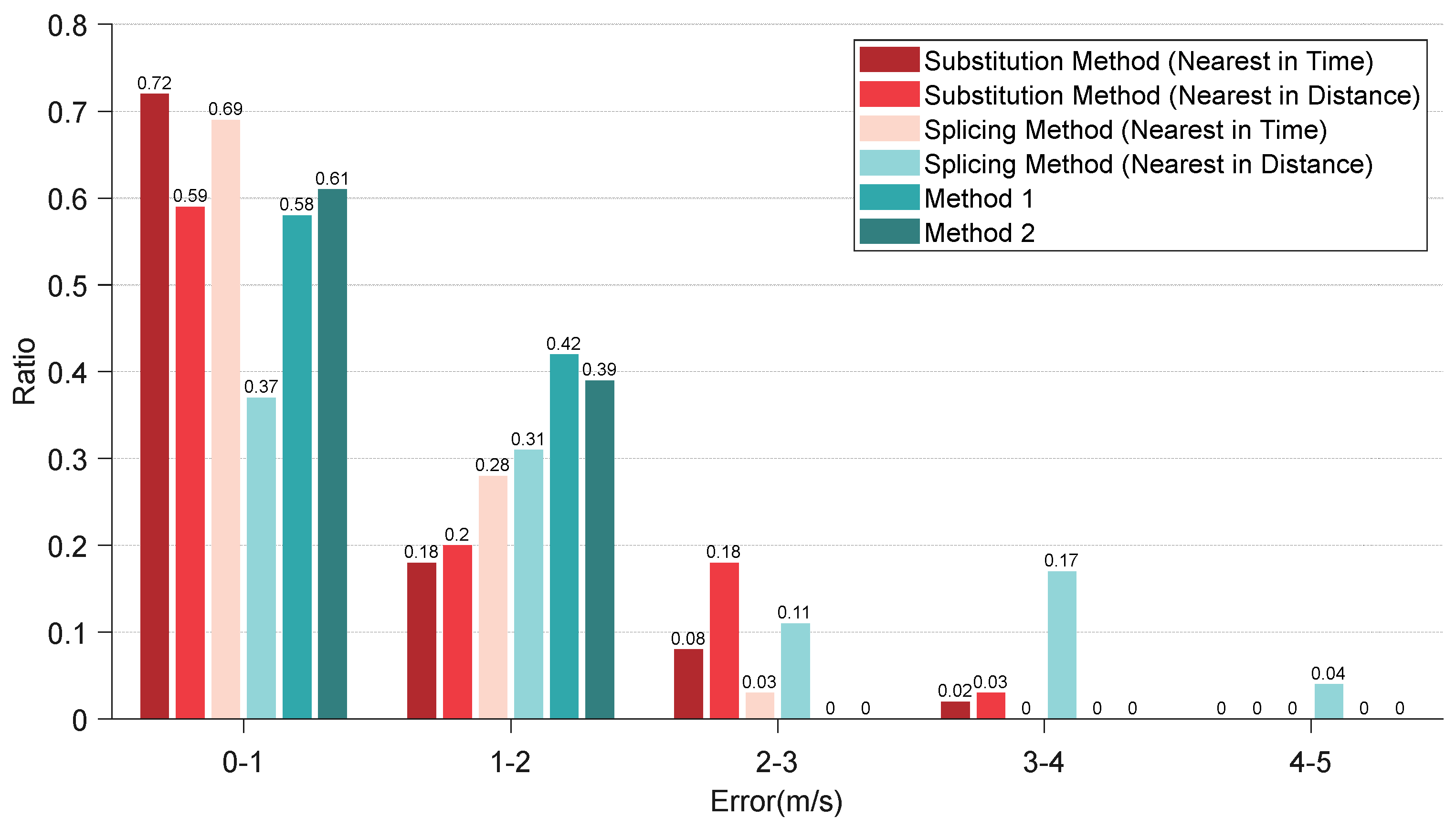
4.1. Analysis of Reconstruction Results with Fixed Sampling Depth of the Measured Sound Speed Profile
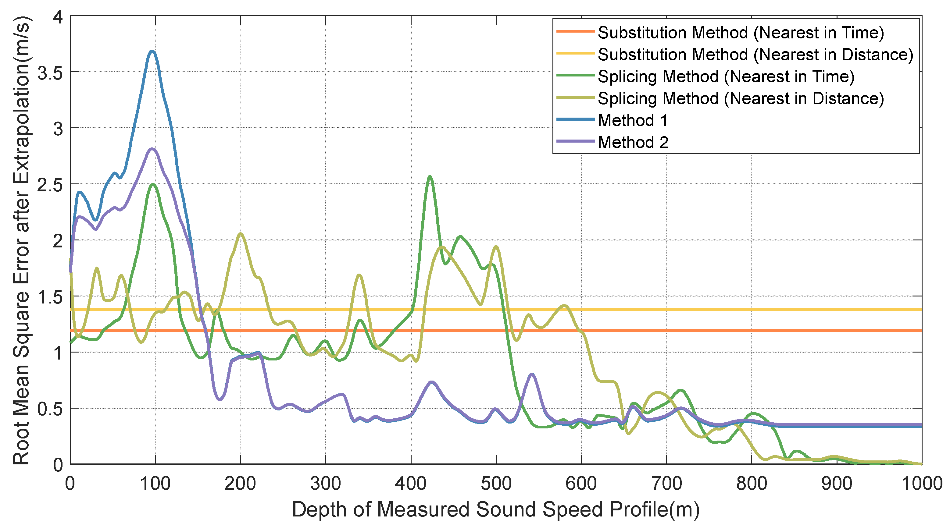
4.2. Analysis of Reconstruction Results with Variable Sampling Depth of the Measured Sound Speed Profile
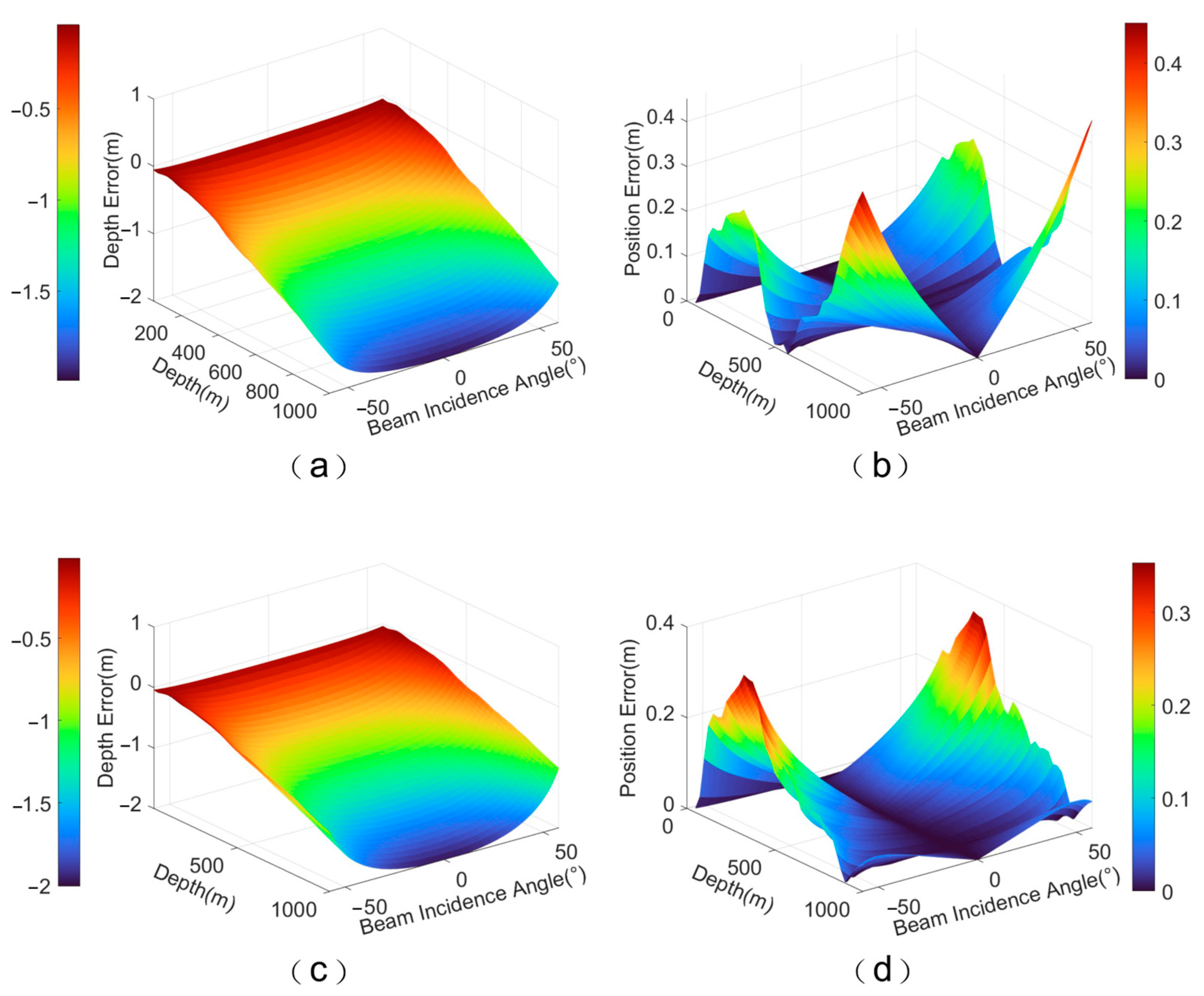
4.3. Analysis of Sound Ray Tracing Results
5. Conclusions
Author Contributions
Funding
Institutional Review Board Statement
Informed Consent Statement
Data Availability Statement
Conflicts of Interest
References
- Li, J. Multibeam Survey Principles, Techniques and Methods; Ocean Press: Beijing, China, 1999; ISBN 7-5027-4834-2. [Google Scholar]
- He, G.W.; Liu, F.L.; Yu, P.; Yang, S.X.; Zhang, Z.R.; Zhao, Z.B. Sound Velocity Correction of Multibeam Bathymetric Systems. Mar. Geol. Quat. Geol. 2000, 4, 109–114. [Google Scholar] [CrossRef]
- Dong, Q.L.; Han, H.Q.; Fang, Z.B.; Pan, L.; Chen, Y.Y.; Lu, G.F. The Influence of Sound Speed Profile’s Correction on Multibeam Survey. Hydrogr. Surv. Charting 2007, 27, 56–58. [Google Scholar]
- Li, J.B.; Zheng, Y.L.; Wang, X.B.; Wu, Z.Y. Main Factors Affecting Multibeam Bathymetric Survey Accuracy. Hydrogr. Surv. Charting 2001, 26–32. Available online: https://kns.cnki.net/KCMS/detail/detail.aspx?dbcode=CJFD&dbname=CJFD2001&filename=HYCH200101005&v= (accessed on 21 March 2024).
- Liu, S.X.; Qu, X.J.; Gao, P.L. New New Idea for the Accuracy of Multibeam Affected by SVP. Hydrogr. Surv. Charting 2008, 28, 31–34. [Google Scholar]
- Zhao, J.H.; Liu, J.N. Multibeam Bathymetric Survey and Image Data Processing; Wuhan University Press: Wuhan, China, 2008; ISBN 978-7-307-06500-0. [Google Scholar]
- Meng, S. Discussion on the Influence of Sound Velocity on Multibeam Bathymetric Measurement and Countermeasures. Ship Supplies Mark. 2019, 6, 20–21. [Google Scholar] [CrossRef]
- Huang, C.H.; Zhang, W.D.; Zhang, Q.L.; Wang, C.; Shen, J.S.; Lu, X.P.; Huang, X.Y. Reconstruction of Full-depth Sound Velocity Profile by Joint WOA2018 Temperature-Salinity Model and In-situ Temperature-Salinity Data (I): Demand Analysis and Technical Scheme. Mar. Surv. 2020, 40, 24–29. [Google Scholar]
- Zhang, Q.G.; Chen, X.; Liu, Q. Research on Sound Velocity Profile Acquisition Method in Remote Multibeam Bathymetric Survey. Mar. Surv. 2019, 39, 1–4. [Google Scholar]
- Huang, C.H.; Lu, X.P.; Ye, A.N.; Luo, S.R.; Huang, X.Y.; Ge, Z.X. Quality Check and Evaluation of Seafloor Topography Measurement Results (II): Acquisition of Sound Velocity Profiles in Deep-sea Areas. Mar. Surv. 2017, 37, 12–16+20. [Google Scholar]
- Zhang, Y.F.; Cheng, D.; Li, S.Q.; Wu, D.S. Research on Sound Velocity Profile Acquisition Method in Deep-sea Areas with Multi-beam Bathymetric Survey. Mar. Surv. 2020, 40, 27–31. [Google Scholar]
- NOAA. NOS Hydrographic Surveys Specifications and Deliverables; NOAA: Silver Spring, MD, USA, 2021. [Google Scholar]
- Huang, C.H.; Wang, Z.; Zhang, X.J.; Yao, J.J.; Li, Z.Q.; Shen, J.S.; Lu, X.P. Reconstruction of Full-depth Sound Velocity Profile by Joint WOA2018 Temperature-Salinity Model and In-situ Temperature-Salinity Data (II): Accuracy Evaluation. Mar. Surv. 2020, 40, 9–14. [Google Scholar]
- Kammerer, E. A New Method for the Removal of Refraction Artifacts in Multibeam Echosounder Systems. Doctoral Dissertation, University of New Brunswick, Fredericton, NB, Canada, 2000. [Google Scholar]
- Wu, T.Y.; Xiao, F.M.; Liu, Y.C.; Zhu, X.C. The Method for Sound Velocity Profile Extrapolation. In Proceedings of the China Society of Surveying and Mapping, Marine Surveying and Mapping Professional Committee, Chengdu, China, 13 September 2009; pp. 227–230. Available online: https://kns.cnki.net/KCMS/detail/detail.aspx?dbcode=CPFD&dbname=CPFD0914&filename=CMJH200909001058&v= (accessed on 21 March 2024).
- Munk, W.H. Sound Channel in an Exponentially Stratified Ocean, with Application to SOFAR. J. Acoust. Soc. Am. 1974, 55, 220–226. [Google Scholar] [CrossRef]
- Davis, T.M.; Count, R.; Yman, K.A.; Carron, M.J. Tailored Acoustic Products Utilizing the NAVOCEANO GDEM (a Generalized Digital Environmental Model). In Proceedings of the 36th Naval Symposium on Underwater Acoustics, San Diego, CA, USA, 1–3 April 1986; pp. 127–131. [Google Scholar]
- Zhang, X.; Zhang, Y.G.; Zhang, J.X.; Dong, N. A New Parametric Method for Sound Velocity Profile. Acta Oceanol. Sin. (Chin. Ed.) 2011, 33, 54–60. [Google Scholar] [CrossRef]
- LeBlanc, L.R.; Middleton, F.H. An Underwater Acoustic Sound Velocity Data Model. J. Acoust. Soc. Am. 1980, 67, 2055–2062. [Google Scholar] [CrossRef]
- Park, J.C.; Kennedy, R.M. Remote Sensing of Ocean Sound Speed Profiles by a Perceptron Neural Network. IEEE J. Ocean. Eng. 1996, 21, 216–224. [Google Scholar] [CrossRef]
- Shen, Y.H.; Ma, Y.L.; Tu, Q.P.; Jiang, X.Q. Feasibility Study of Representing Shallow Water Sound Velocity Profile Using Empirical Orthogonal Functions (EOF). Appl. Acoust. 1999, 18, 21–25. [Google Scholar]
- Sun, W.C.; Bao, J.Y.; Jin, S.H. Impact of EOF Representation of Sound Velocity Profile on Multibeam Bathymetric Data. Mar. Surv. 2014, 34, 21–24+28. [Google Scholar]
- He, L.; Li, Z.L.; Zhang, R.H.; Li, F.H. Empirical Orthogonal Function Representation and Matching Field Inversion of Sound Velocity Profile in East China Sea. Prog. Nat. Sci. 2006, 16, 351–355. [Google Scholar]
- Zhang, Z.M.; Li, Z.L.; Dai, Q.X. Reconstruction of Full-depth Sound Velocity Profile Using Limited-depth Sound Velocity Data. In Proceedings of the 2008 National Acoustics Conference, Shanghai, China, 22–24 October 2008; p. 2. Available online: https://kns.cnki.net/kcms2/article/abstract?v=p7sfyaWOx3OSCy4rHJ9BblVKlFiMvVsmNEAz0a-IYxHD5Kik5UeHLi7FfvKDR75fC2IKhu3gA9IoNous9oypI2tmZOvOFg7_ZZfYkWntGBK3mSsWrdYeSyjy-lch7GeMuIcUHuRZC12CH00gCG1uVw==&uniplatform=NZKPT&language=CHS (accessed on 21 March 2024).
- Zhang, W.; Huang, Y.W.; Wang, Y.Y. Reconstruction of Sound Velocity Profile Using Incomplete Sample Data. Acoust. Tech. 2012, 31, 371–374. [Google Scholar]
- Cheng, F.; Chen, S.; Jin, S.H.; Sun, W.C. Study on Extrapolation Method of Sound Velocity Profile in Continental Margin Deep Water Area. Mar. Surv. 2016, 36, 26–29. [Google Scholar]
- Yang, F.; Zheng, H.; Zheng, H.; Wang, J.; Kong, L.M.; Xu, K. Analysis of Sound Velocity Structure and Empirical Orthogonal Function Extension in Zhoushan Sea Area. China Water Transp. 2016, 16, 142–144. [Google Scholar]
- Pearson, K. On Lines and Planes of Closest Fit to Systems of Points in Space. Lond. Edinb. Dublin Philos. Mag. J. Sci. 1901, 2, 559–572. [Google Scholar] [CrossRef]
- Davis, R.E. Predictability of Sea Surface Temperature and Sea Level Pressure Anomalies over the North Pacific Ocean. J. Phys. Oceanogr. 1976, 6, 249–266. [Google Scholar] [CrossRef]
- Nie, G.G.; Wan, J.H. Application of Akima Interpolation Method in Measurement. Surv. Technol. News 1998, 31–34. Available online: https://kns.cnki.net/kcms2/article/abstract?v=6xaVI2TORM3dHWE9xfyhgc32MqFWacD09temugaiNPMKdrIL9q3lhHKiKPOk7rD2YXP-oJbiPzLOdm57cRLlvtWrpCz8tajgWLsxHs5IWEBvh04ne-b5Vs0N8GMXy9hW4r3iwk1A-c0=&uniplatform=NZKPT&language=CHS (accessed on 21 November 2023).
- Bica, A.M. Optimizing at the End-Points the Akima’s Interpolation Method of Smooth Curve Fitting. Comput. Aided Geom. Des. 2014, 31, 245–257. [Google Scholar] [CrossRef]
- Abdel-Basset, M.; Mohamed, R.; Abouhawwash, M. Crested Porcupine Optimizer: A New Nature-Inspired Metaheuristic. Knowl.-Based Syst. 2024, 284, 111257. [Google Scholar] [CrossRef]
- Zhou, F.N.; Zhao, J.H.; Zhou, C.Y. Determination of Classic Experiential Sound Speed Formula in Multibeam Echo Sounding System. J. Oceanogr. Taiwan Strait 2001, 20, 411–419. [Google Scholar]
- Ding, J.S.; Zhou, X.H.; Tang, Q.H.; Liu, Z.C.; Chen, Y.L. Correction Technique of Sound Ray Refraction for Multibeam Echo Sounder System Based on Equivalent Sound Velocity Profile Method. Hydrogr. Surv. Charting 2004, 24, 27–29. [Google Scholar]
- Fang, W.M. Research on Sound Velocity Correction Method Based on Equivalent Sound Velocity Profile Method and Its Improved Model. China Water Transp. 2013, 13, 72–73. [Google Scholar]
- Wang, J. Research on Sound Velocity Correction Method for Multibeam Echo Sounder. Master’s Thesis, China University of Petroleum (East China), Qingdao, China, 2012. [Google Scholar]
- Qi, N.; Tian, T. Sound Ray Tracking Technology in Multibeam Swath Bathymetry. J. Harbin Eng. Univ. 2003, 24, 245–248. [Google Scholar]
- Lu, X.P.; Bian, S.F.; Huang, M.T.; Zhai, G.J. Improved Algorithm for Average Sound Velocity in Constant Gradient Sound Ray Tracking. J. Wuhan Univ. (Inf. Sci. Ed.) 2012, 37, 590–593. [Google Scholar] [CrossRef]
- IHO. IHO Standards for Hydrographic Surveys, 6th ed.; Special Publication No. 44; IHO: Monaco City, Monaco, 2020. [Google Scholar]
- Zhu, X.C. Research on Key Models and Applications of Multibeam Echo Sounder Data Processing; Dalian Naval Academy: Dalian, China, 2011. [Google Scholar]
Disclaimer/Publisher’s Note: The statements, opinions, and data contained in all publications are solely those of the individual author(s) and contributor(s) and not of MDPI and/or the editor(s). MDPI and/or the editor(s) disclaim responsibility for any injury to people or property resulting from any ideas, methods, instructions, or products referred to in the content. |


| Tested Sound Speed Profile | Sound Speed Profile Nearest in Time | Sound Speed Profile Nearest in Location | |
|---|---|---|---|
| Measurement Time | 15 February 2006 | 15 February 2006 | 20 February 2006 |
| Measurement Location | 24.878° N, 136.277° E | 24.139° N, 135.298° E | 24.983° N, 136.347° E |
| Mode | Eigenvalue | Variance Contribution Ratio (%) | Cumulative Variance Contribution Ratio (%) |
|---|---|---|---|
| 1 | 1996.14 | 52.82 | 52.82 |
| 2 | 1112.03 | 29.43 | 82.25 |
| 3 | 260.00 | 6.88 | 89.13 |
| 4 | 105.77 | 2.80 | 91.93 |
| 5 | 62.05 | 1.64 | 93.57 |
| 6 | 49.51 | 1.31 | 94.88 |
| 7 | 39.40 | 1.04 | 95.92 |
| Mode | Eigenvalue | Variance Contribution Ratio (%) | Cumulative Variance Contribution Ratio (%) |
|---|---|---|---|
| 1 | 1978.36 | 52.15 | 52.15 |
| 2 | 1138.46 | 30.01 | 82.16 |
| 3 | 265.35 | 6.99 | 89.15 |
| 4 | 108.29 | 2.85 | 92.00 |
| 5 | 58.68 | 1.55 | 93.55 |
| 6 | 50.22 | 1.32 | 94.87 |
| 7 | 39.04 | 1.03 | 95.90 |
| Mode | 1 | 2 | 3 | 4 | 5 | 6 | 7 |
|---|---|---|---|---|---|---|---|
| Upper Bound | 71.42 | 76.94 | 37.33 | 22.85 | 15.28 | 15.75 | 18.48 |
| Lower Bound | −92.15 | −80.40 | −42.00 | −15.67 | −22.16 | −18.40 | −16.19 |
| Order | 1 | 2 | 3 | 4 | 5 | 6 | 7 |
|---|---|---|---|---|---|---|---|
| Method 1 | 52.8544 | 1.4062 | 6.0237 | −0.1497 | −13.4213 | 5.1578 | −8.0620 |
| Method 2 | 51.8908 | 1.2862 | 5.9058 | −0.1643 | −14.8596 | 3.7157 | −6.6353 |
| Nearest Substitution Method | Nearest Splicing Method | Method 1 | Method 2 | |||
|---|---|---|---|---|---|---|
| Time Nearest | Location Nearest | Time Nearest | Location Nearest | |||
| RMSE (m/s) | 1.1938 | 1.3802 | 0.9975 | 2.0551 | 0.9594 | 0.9511 |
| MAE (m/s) | 0.8638 | 1.0548 | 0.7739 | 1.5959 | 0.8510 | 0.8492 |
| MAPE (%) | 0.0574 | 0.0701 | 0.0517 | 0.1064 | 0.0568 | 0.0566 |
| R2 | 0.9942 | 0.9922 | 0.9959 | 0.9827 | 0.9962 | 0.9963 |
| Nearest Substitution Method | Nearest Splicing Method | Method 1 | Method 2 | |||
|---|---|---|---|---|---|---|
| Time Nearest | Location Nearest | Time Nearest | Location Nearest | |||
| Maximum (m/s) | 3.7194 | 3.1448 | 2.6747 | 4.2695 | 1.9417 | 1.9325 |
| Minimum (m/s) | −1.7867 | −1.1246 | −2.0204 | 0 | −1.0022 | −1.2678 |
| Mean (m/s) | 0.5180 | 0.8037 | −0.3053 | 1.5959 | 0.7673 | 0.7445 |
Disclaimer/Publisher’s Note: The statements, opinions and data contained in all publications are solely those of the individual author(s) and contributor(s) and not of MDPI and/or the editor(s). MDPI and/or the editor(s) disclaim responsibility for any injury to people or property resulting from any ideas, methods, instructions or products referred to in the content. |
© 2024 by the authors. Licensee MDPI, Basel, Switzerland. This article is an open access article distributed under the terms and conditions of the Creative Commons Attribution (CC BY) license (https://creativecommons.org/licenses/by/4.0/).
Share and Cite
Zhang, W.; Jin, S.; Bian, G.; Peng, C.; Xia, H. A Method for Full-Depth Sound Speed Profile Reconstruction Based on Average Sound Speed Extrapolation. J. Mar. Sci. Eng. 2024, 12, 930. https://doi.org/10.3390/jmse12060930
Zhang W, Jin S, Bian G, Peng C, Xia H. A Method for Full-Depth Sound Speed Profile Reconstruction Based on Average Sound Speed Extrapolation. Journal of Marine Science and Engineering. 2024; 12(6):930. https://doi.org/10.3390/jmse12060930
Chicago/Turabian StyleZhang, Wei, Shaohua Jin, Gang Bian, Chengyang Peng, and Haixing Xia. 2024. "A Method for Full-Depth Sound Speed Profile Reconstruction Based on Average Sound Speed Extrapolation" Journal of Marine Science and Engineering 12, no. 6: 930. https://doi.org/10.3390/jmse12060930
APA StyleZhang, W., Jin, S., Bian, G., Peng, C., & Xia, H. (2024). A Method for Full-Depth Sound Speed Profile Reconstruction Based on Average Sound Speed Extrapolation. Journal of Marine Science and Engineering, 12(6), 930. https://doi.org/10.3390/jmse12060930