Abstract
A numerical model for the simulation of the performance of an oscillating water column (OWC) subjected to non-breaking and breaking waves is proposed in this paper. The numerical model consists of a hydrodynamic model specifically designed to simulate breaking waves and a pneumatic model that takes into account the air compressibility. The proposed numerical model was applied to evaluate the potential mean annual energy production from the waves of two coastal sites characterized by different hydrodynamic conditions: a deep-water condition, where the OWC interacts with non-breaking waves, and a shallow-water condition, where the OWC is subjected to breaking waves. The numerical results show that the effects of the air compressibility can be considered negligible only in numerical simulations of the performances of reduced-scale OWC devices, such as those used in laboratory experiments. We demonstrated that in real-scale simulations, the effect of the air compressibility within the OWC chamber significantly reduces its ability to extract energy from waves. The numerical results show that the effect of the air compressibility is even more significant in the case of a real-scale OWC located in the surf zone, where it interacts with breaking waves.
1. Introduction
In coastal regions, gravity wave motion can be an important alternative renewable source for the production of electric energy. Among the simplest devices for the conversion of wave energy to electric energy are bottom-fixed oscillating water columns (OWCs) [1]. The main structural element of these devices is a semi-submerged chamber fixed to the bottom, with three closed sides and one open side oriented toward the direction of prevailing waves. The lower part of the chamber is occupied by water in direct contact with the sea; the upper part of the chamber is occupied by air, which is connected to the external environment by a pipe that forces it to pass through a turbine. Due to the wave motion, the water in the lower part of the chamber behaves as an oscillating column, which, during its upward movement, pushes the air out of the chamber and draws air inside during its downward movement. The adoption of a self-rectifying turbine (which rotates in the same sense regardless of the air flow direction) allows the OWC to produce electric energy during all phases of a wave’s motion [2]. The assessment of the potential capacity of a coastal site to extract energy from waves requires the simulation of the complex interaction between the prevailing waves and the OWC. The complexity of this phenomenon is due to the mutual interaction between the wave motion outside and inside the chamber and the transit of the air through the turbine. In fact, the wave motion inside the chamber produces air volume variations and a consequent transit of air though the turbine; in turn, the air transit through the turbine causes a pressure jump between upstream and downstream and consequent overpressure or underpressure conditions within the chamber, depending on whether the air exits or enters. Overpressure conditions within the chamber can favor the descending phase of the waves and hinder the ascending one, while underpressure conditions inside the chamber can have the opposite effect. The simulation of these mutual interactions is necessary to evaluate the capacity of a given OWC to extract energy from waves for the different characteristics of the OWC chamber and wave fields. The above-mentioned simulations can be carried out by laboratory experiments [3,4,5] and numerical models [6,7,8,9]. Laboratory tests have the advantage of being able to actually reproduce, albeit on a smaller scale, the physical behavior of a given OWC prototype subjected to a certain wave field. The main disadvantages of this approach are the difficulties of reproducing real-scale phenomena and modifying the chamber geometry and wave characteristics.
On the other hand, numerical models have the advantage of being able to simulate even real-scale phenomena and to easily modify the chamber geometry and wave conditions, making it easier to investigate different OWC operating scenarios. The main disadvantage of this approach is the fact that numerical models reproduce real phenomena in a virtual way with a degree of approximation that is related to the simplifications introduced in the mathematical models and numerical methods. Numerical models for the study of OWC performances usually consist of two main sub-models: a hydrodynamic model for the simulation of water velocity fields and free-surface elevations due to the wave motion; and a pneumatic model, for the simulation of pressure air variations inside the chamber due to the transit of air through the turbine.
In several numerical studies on the hydrodynamic performance of OWCs, the adopted hydrodynamic model is based on the potential flow theory [6,7,8]. Such hydrodynamic models are mainly suitable for the simulation of non-breaking waves that propagate in deep water and, consequently, have good agreement with the experimental data of OWCs located outside the breaking zone. In the case of numerical studies of OWCs located inside the breaking zone or in shallow water, more complex hydrodynamic models are needed, such as those based on the numerical integration of the Navier–Stokes equations by shock-capturing numerical schemes [10,11,12]. This approach has been used in a recent study [13], in which some of the present authors made a comparison between the performances of an OWC subjected to regular waves and those obtained by using irregular waves characterized by the same wave energy. The results of the above-mentioned study demonstrated that the hydrodynamic efficiency of an OWC calculated by using irregular waves (which represent marine wave motion more realistically) is significantly lower than that calculated by using regular waves. As demonstrated in the present work, the evaluation of the OWC efficiency obtained in [13] (although more realistic than that obtained by using regular waves) may still be overestimated because it was calculated by a pneumatic model that is usually adopted in the literature [7,8,9,13], in which the simplifying hypothesis of air incompressibility was assumed. This hypothesis is fully justified only in the case of low air speeds, i.e., a low rate of change in the air volume in the OWC chamber. More sophisticated pneumatic models have recently been proposed in the literature to take into account the effect produced on OWC performances by the compressibility of the air in the chamber [14,15,16]. In such models, the spatial variations in the air characteristics over the chamber are neglected, and a single time-varying value of the air density and pressure inside the chamber is calculated during the simulation. By this approach, a practical model to take into account the air compressibility without excessively increasing the complexity of the numerical model can be obtained.
In the present paper, we present a development of the work of Cannata et al. [13]. We propose a pneumatic model that overcomes the simplifying hypothesis of air incompressibility, and we evaluate the performances of an OWC in two different hydrodynamic conditions, one characterized by non-breaking waves and one by breaking waves. The proposed numerical model consists of two sub-models: (a) a hydrodynamic model in which the Navier–Stokes equations are numerically integrated by a recently proposed shock-capturing numerical scheme that is specifically designed to simulate breaking waves [17]; and (b) a pneumatic model based on the thermodynamic equations proposed in [16], which takes into account the effect of air compressibility on the pressure variations in the chamber.
The proposed numerical model was validated by experimental tests on a laboratory-scale OWC and was applied to the simulation of the performances of a real-scale OWC in two sites on the Italian coast that are characterized by different hydrodynamic conditions. The first set of numerical simulations concerned the performances of a large OWC that is located on the external side of the new breakwater for the protection of the Genoa harbor in a deep-water region (water depth equal to 50 m), where the OWC is subjected to non-breaking waves. The second set of numerical simulations regarded the performances of an OWC that is located on the external side of a T-groin for the protection of the coast of Paola (in southern Italy) in a shallow-water region (water depth equal to 3 m), where the OWC is subjected to breaking waves.
The above-mentioned simulations were carried out both by the proposed numerical model and by a simplified version that is based on the assumption, usually adopted in the literature [8,9,10], of the incompressibility of air. The comparison between the two sets of numerical results allows us to highlight the limits of the applicability of the simplified pneumatic model, which become evident when moving from the laboratory scale to the real scale and are more significant in the case of breaking waves. This paper is organized as follows. In Section 2, we present, in a synthetic way, the equations of the hydrodynamic model, and we extensively derive the equations of the pneumatic model. In Section 3, the proposed model is validated against experimental tests and is applied to the assessment of the energy production from waves in two sites on the Italian coast characterized by different hydrodynamic conditions. Conclusions are drawn in Section 4.
2. Materials and Methods
The proposed numerical model consists of two sub-models: a hydrodynamic sub-model for the simulation of the water velocity fields and free-surface elevations due to wave motion; and a pneumatic sub-model for the simulation of the variations in the pressure in the OWC chamber due the transit of air through the turbine.
2.1. Hydrodynamic Model
In the proposed hydrodynamic sub-model, the water velocity and free-surface elevations are obtained by numerically integrating the Navier–Stokes equations (expressed in an integral and contravariant formulation) on moving curvilinear coordinates that follow the free-surface oscillations [12]. In a two-dimensional vertical space, where is the horizontal Cartesian coordinate and is the vertical one, we define the following time-dependent coordinate transformation:
in which is the total water depth, given by the sum of the still water depth, , and the free-surface elevation, . By indicating with the generic covariant base vectors, with the generic contravariant base vectors, and with the specific contravariant base vector defined at the centre the generic calculation cell of area , the system of motion equations read as follows:
where and are the averaged values, respectively, over the one-dimensional and two-dimensional grid cell of the conserved variables and ; are, respectively, the contravariant components of the water and grid points’ velocity; are the contravariant components of the strain rate tensor; is the dynamic pressure component; is the acceleration due to gravity; is the eddy viscosity (that is calculated by the Smagorinsky sub-grid scale model); indicate the border points of the one dimensional grid cell, which are located on the higher and lower values of ; and , indicate the contour lines of the two-dimensional calculation grid (on which is constant), which are located on the higher and lower values of . Equations (2) and (3) are numerically integrated by a finite-volume shock-capturing scheme specifically designed to simulate breaking waves [17].
2.2. Pneumatic Model
In the proposed pneumatic sub-model, we take into account the air compressibility within the OWC chamber. To this end, we follow the line proposed by [16] and represent the air column inside the OWC chamber as an open thermodynamic system consisting of a perfect gas that exchanges matter and energy with its surroundings. The exchanges of matter are due to air passages (incoming and outgoing) through the turbine between the chamber and the external environment. The exchanges of energy are due (to a lesser extent) to the energy of the gas exchanged with the environment and (to a greater extent) to the work carried out by the air column on the water column below (and vice versa) during the oscillatory motion. For this thermodynamic system, at the generic instant , the total energy, , can be expressed by the sum of the internal energy, , the kinetic energy, , and the potential energy, . By using the first principle of thermodynamics and neglecting the variations in the potential and kinetic energy of the gas and the exchanges of heat with the external environment, the rate of change in the total energy of the open system, , can be written as [18]
where is the amount of energy exchanged, per unit time, in the form of work, between the system and the environment (positive if transferred to the system); is the mass flow rate that at instant is exchanged between the system and the environment (positive if entering the system); and is its enthalpy per unit mass. In the present case, the amount of work per unit time on the right-hand side of Equation (4) reads as follows:
in which and are, respectively, the pressure and time rate of change in the volume of the gas inside the chamber. The enthalpy of the air mass exchanged per unit time on the right-hand side of Equation (4) is obtained by using the relationship between the infinitesimal variations in the enthalpy of a fixed amount of perfect gas, , and the temperature variations,
where the number of moles, is expressed by the ratio between the mass and molar mass , and is the specific molar heat capacity at a constant pressure. By integrating the above equation by parts and multiplying the result by , the last term on the right-hand side of Equation (4) reads as follows:
The left-hand side of Equation (4) is obtained by the equation between the infinitesimal variations in the internal energy of a fixed amount of perfect gas, , and the variations in the temperature,
where is the specific molar heat capacity at a constant volume. By integrating the above equation by parts, we obtain the dependence of the internal energy of a perfect gas on the temperature,. The latter equation is then used to obtain the rate of change in the internal energy of an amount of perfect gas in which, in addition to the temperature, the mass also varies.
By substituting the expressions on the right-hand side of Equations (5), (7) and (9), into Equation (4), we have
By multiplying Equation (10) by and using the adiabatic dilatation coefficient, and Meyer’s equation, (where is the constant of perfect gases), Equation (10) reads as follows:
In order to express the temperature-dependent terms of Equation (11) (left-hand side and last term on the right-hand side) as a function of pressure and volume, we use the equation of state of perfect gases (in which the number of moles is substituted by the ratio )
In fact, by deriving Equation (12) with respect to time, we obtain
By expressing by Equation (13) and by Equation (12), substituting them into Equation (11), and dividing by we obtain
The next step is to express the ratio on the right-hand side of Equation (14) as a function of the air flow rate that passes through the turbine, . By following the convention adopted in [16], we consider the air flow rate exiting the chamber to be positive and the one entering from the external environment to be negative (both passing through the turbine). By indicating the density of the external air with and the air inside the chamber with , the ratio on the right-hand side of Equation (14) reads as follows:
By introducing a coefficient , whose value is if and if , the two conditions for can be written in the following form:
By substituting the right-hand side of Equation (16) into Equation (14) and assuming the typical linear relationship between the air flow rate through the Wells turbine and the pressure difference between upstream and downstream, (where is the turbine constant), and Equation (14) reads as follows:
Equation (17) allow us to express the variations in the air pressure within the chamber as a function of the variations in the air volume and density. Since the volume variations are calculated by the hydrodynamic model, it is sufficient to introduce a relationship between the air density and pressure to close the system of equations of the pneumatic model. To this end, we use the well-known relationship for isentropic transformations, , which, when written in differential form, reads as follows:
The system of Equations (17) and (18) is solved, together with the equations of the hydrodynamic model, by an explicit scheme that is second-order in time. Once the pressure is updated, the instant power absorbed by the turbine, , is given by
This pneumatic model is two-way coupled with the hydrodynamic model described in Section 2.1; at every instant of the simulation, the updating of the air pressure within the chamber is carried out by Equation (17), in which the air density is updated by Equation (18), and the air volume and its rate of change are calculated by the hydrodynamic model at the previous time step; in turn, the hydrodynamic model adopts the air pressure calculated by Equation (17) as a boundary condition on the free surface within the air chamber. This coupling allows us to simulate the mutual interaction between the passages of the waves from outside to inside the chamber and the transit of the air through the turbine.
The wave motion that is transmitted inside the chamber produces the variations in the air volume that induce its transit through the turbine; in turn, the air transit through the turbine produces a pressure jump between upstream and downstream that can favor or hinder the wave motion within the chamber. The simulation of this mutual interaction allows us to assess the ability of an OWC to absorb energy from waves for different OWC geometrical characteristics and wave conditions.
3. Results and Discussion
3.1. Validation
The validation of the proposed model was carried out by numerically reproducing the set of laboratory experiments performed by Morris-Thomas et al. [3], which are usually adopted to verify the ability of numerical models to simulate the interactions between waves and OWCs. These laboratory tests were carried out on a 1:12.5 scale model of an existing OWC. The length of the OWC chamber was , and the still water depth was . The turbine constant was 396. In each laboratory test, the input waves were regular wave trains with a fixed wave height, , and a different wave period (to which a different wavelength corresponded). For each laboratory test, the average power absorbed by the OWC was experimentally measured and divided by the theoretical energy transmitted per unit time by the given undisturbed wave. This ratio, which is between 0 and 1, gives the hydrodynamic efficiency, of the OWC as the period (or wavelength) of the input waves varies.
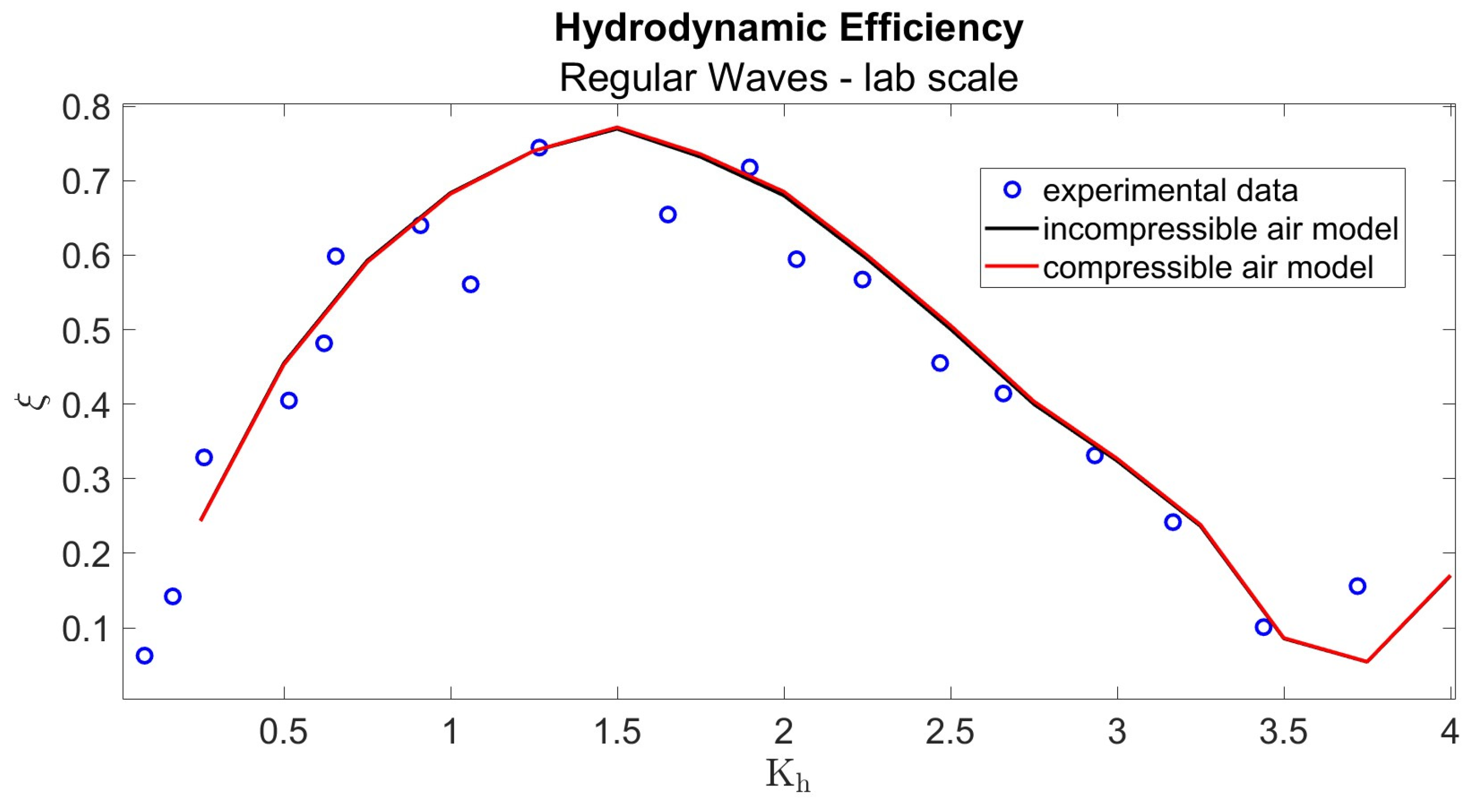
In the present work, the above experimental tests were numerically reproduced by using both the proposed model (hereinafter called the compressible air model) and a simplified version obtained by assuming the incompressibility of the air within the OWC chamber (hereinafter called the incompressible air model). All the numerical simulations were carried out by a moving calculation grid, where the horizontal grid step was , the number of grid cells along the vertical direction was , and the time step was , which guaranteed a Courant–Levy–Fredericks number, , of always less than in order to avoid numerical instabilities. For every case, the simulation duration exceeded 100 wave periods (or peak spectrum periods in the case of irregular waves). The error estimate in every numerical simulation was calculated by the root mean square error, , where and are, respectively, the experimental and corresponding numerical values. Figure 1 shows the comparison between the experimental results obtained by [3] and those obtained by the compressible air model and the incompressible air model. In this case, the root mean square errors were both very low and were, respectively, and . The figure shows the variation in the OWC’s hydrodynamic efficiency as the non-dimensional wave number, , varied, where is the wavenumber and is the still water depth. The experimental measurements show that in the laboratory-scale OWC, the interactions with regular waves whose non-dimensional wave numbers were close to (corresponding to a wavelength ) produced a peak of hydrodynamic efficiency. As demonstrated in a previous work [13], such an efficiency peak is due to resonance phenomena, in which the pressure oscillations within the chamber favor free-surface oscillations and induce their amplification.
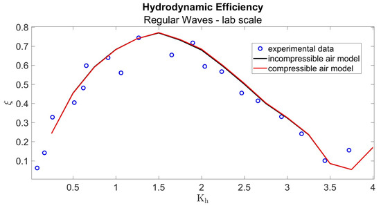
Figure 1.
Hydrodynamic efficiency of a laboratory-scale OWC. Comparison between experimental measurements by [3] (circles), numerical results obtained by the proposed compressible air model (red line), and those obtained the incompressible air model (black line).
The very good agreement between the experimental results and those obtained by both numerical models, which is shown in Figure 1 and was quantified by the very low root mean square errors, demonstrates that for those simulations, the adoption of a simplified pneumatic sub-model was fully justified. In fact, in the case of the laboratory-scale OWC (where the chamber dimensions and wave height were of the order of centimetres), the rate of change in the air volume within the chamber and the speed of the air were so low as to make the effect of the air compressibility negligible.
It must be emphasized that in the case of a large OWC, such as real-scale ones, the rate of change in the air volume and air speed through the turbine can be an order of magnitude higher than those measured in laboratory-scale models. For such real-scale OWCs, the compressibility of the air within the chamber can have a non-negligible effect on the hydrodynamic performance.
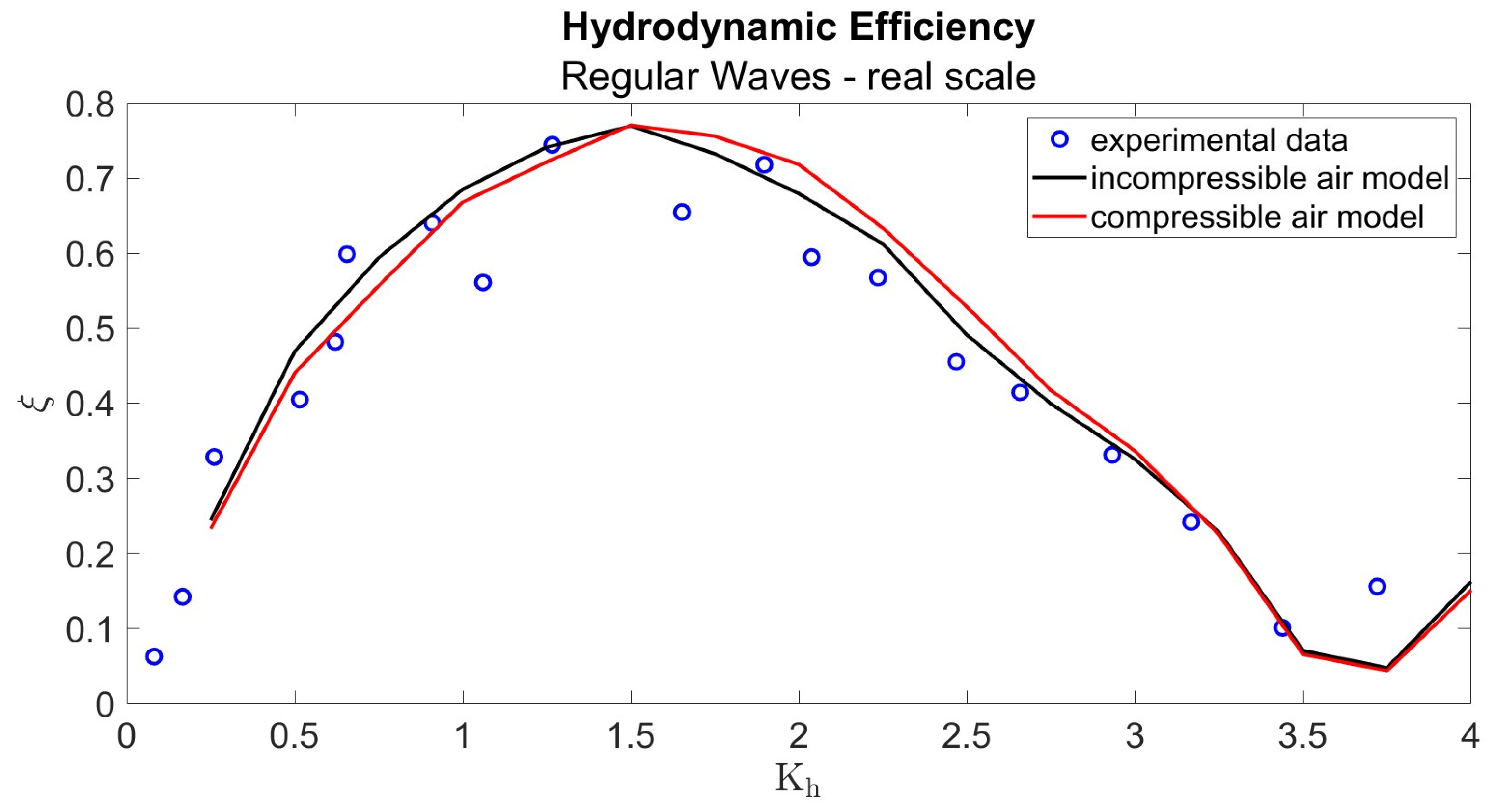
In order to evaluate the effect produced by air compressibility on real-scale OWC performances, in Figure 2, we show the results of a further set of numerical simulations that were carried out by numerically reproducing the real-scale OWC from which the scale model used in the laboratory tests was taken. In those real-scale numerical simulations, the OWC dimensions and the characteristics of the input waves were obtained from the laboratory-scale ones by using the well-known Froude similitude laws. In this way, we numerically simulated the performances of a real-scale OWC subjected to regular waves with a wave height of and a variable wave period between and . These simulations were carried out both by the proposed model (which takes into account the air compressibility) and by the simplified one (in which the air is assumed to be incompressible). As can be seen from Figure 2, the transition from the laboratory-scale dimensions to the real-scale ones involved differences in the numerical results obtained by the two different models that were no longer negligible. In this case, the differences in the OWC’s hydrodynamic efficiency produced by the two different models were approximately 5%.

Figure 2.
Hydrodynamic efficiency of a real-scale OWC. Comparison between experimental measurements by [3] (circles), numerical results obtained by the proposed compressible air model (red line), and those obtained the incompressible air model (black line).
As we demonstrate in the next section, in the numerical simulations regarding a real-scale OWC subjected to irregular waves (that reproduced the wave conditions in a more realistic way than the regular waves used in the laboratory tests), the OWC’s hydrodynamic performances obtained by the compressible air model were significantly worse than those obtained by the incompressible air model. It must be emphasized that these results are justified by theoretical considerations but are not supported by experimental data, since, to the authors’ knowledge, no laboratory experiments are available for such real-scale conditions.
3.2. Real Cases Applications
In this section, the proposed model is applied to assess the potential production of energy from waves of two Italian coastal sites characterized by different hydrodynamic conditions. The first site is in front of the port of Genoa, on the offshore side of the new breakwater. This breakwater design is located in the deep-water region of the Genova gulf, where the water depth is h = 50 m, and the OWC would be subjected to non-breaking waves at this location. The second site is in front of the coast of Paola, in southern Italy, on the offshore side of T-groin placed to protect the coast from waves. The shoreline-parallel part of the T-groin is located in the surf region, where the water depth is h = 3 m, and the OWC would be subjected to breaking waves at this location.
3.2.1. Performance of an OWC Subjected to Non-Breaking Waves (Genoa Port)
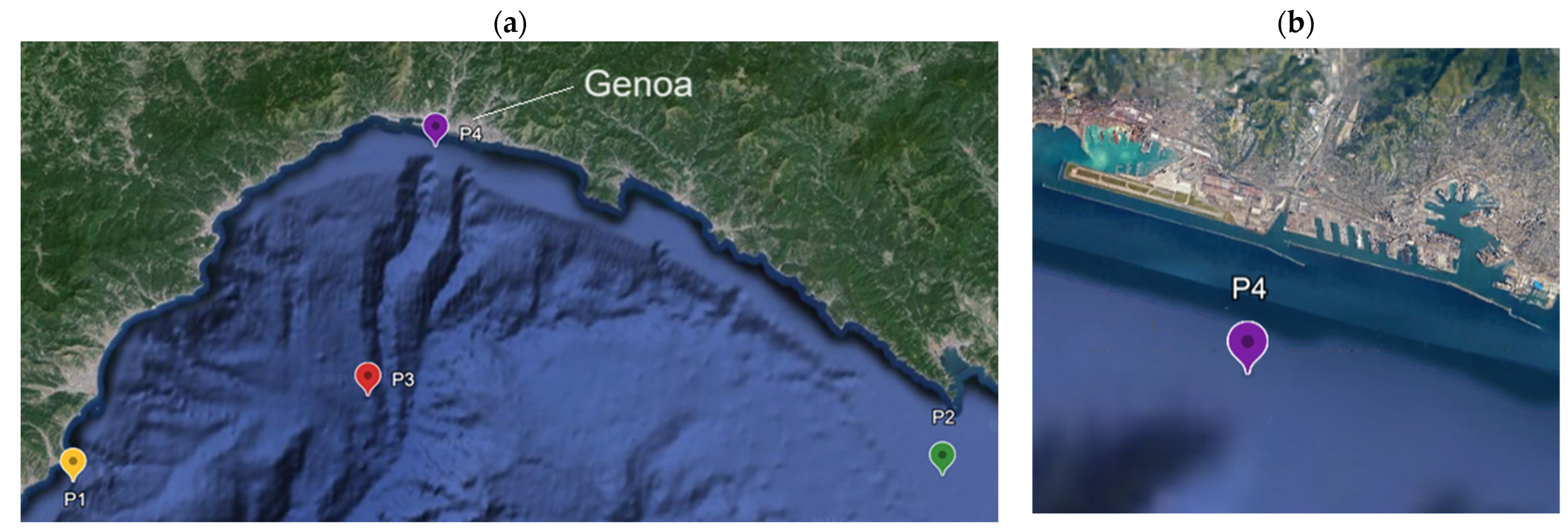
In this section, the results of the numerical simulations of the interactions between an OWC located on the new offshore breakwater of Genoa port and the prevailing waves are shown. The statistical characteristics of the waves were obtained from the meteo-marine study attached to the technical and economic feasibility study of the new offshore breakwater of Genoa port. In absence of direct wave height data measured off the Genoa port, in the above-mentioned study, the authors used a historical series of the wave height measured by two directional wave buoys located at the western and eastern extremes of the Genoa Gulf: the buoy of Capo Mele (point P1 in Figure 3) and the buoy of La Spezia (point P2 in Figure 3). Such data were used in the ERA5 reanalysis to reconstruct the spectral characteristics of a third point located 42 km off the port of Genoa (point P3 in Figure 3). From this point, according to a shoaling and refraction model [19], the waves were propagated to a closer point (point P4 in Figure 3), which is about 1 km away from the port and was the starting point of the numerical simulations carried out by the proposed model. The mean annual wave characteristics at point P4 are shown in Figure 4 and are listed in Table 1. These data were used to build the wave input data of the proposed hydrodynamic model, which were irregular wave trains with JONSWAP spectra, whose significant wave height and peak period are the ones listed in Table 1. For every irregular wave, the input data were the time series of the boundary free-surface elevation and flow velocity obtained by the superposition of sinusoidal waves with different amplitudes and periods, which were derived from the discretized wave spectrum [13]. In this way, we simulated the propagation of the most frequent waves from point P4 to the Genoa port breakwater and we evaluated the mean annual energy production that can be extracted from such waves by an OWC.

Figure 3.
Full (a) and detailed view (b) of the Gulf of Genoa. Point P1: buoy of Capo Mele; point P2: buoy of La Spezia; point P3: reconstructed data point by reanalysis; point P4: starting point of the numerical simulations carried out by the proposed model.

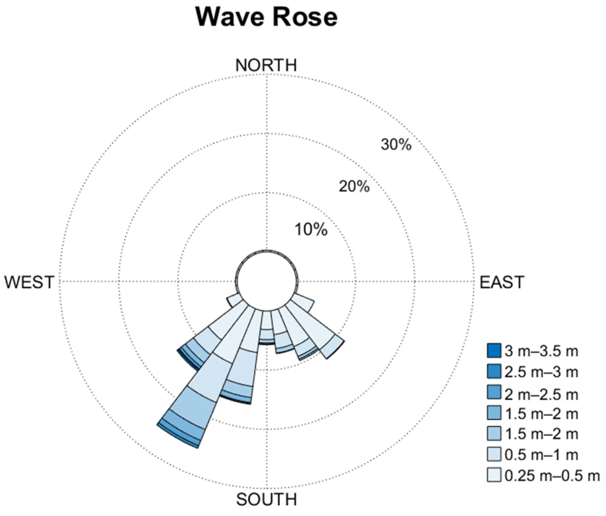
Figure 4.
Wave rose diagram of mean annual significant wave heights of point P4, offshore of Genoa’s port breakwater.

Table 1.
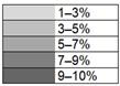
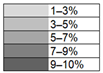
Mean annual wave characteristics of point P4, off the Genoa port breakwater. Angle of direction of origin of the waves ( significant wave height (), mean wave period (number inside the rectangles), and frequency of occurrence of every triplet (gray scale).
In Table 1, we highlight the characteristics of the waves used as the input data of the numerical simulations, which were obtained by dividing the sea states of the reconstructed historical series into classes of significant height, , direction of origin, , and wave period (number inside the rectangles) and calculating the frequency of occurrence of every triplet (gray scale).
The input waves used for this case study were those belonging to the origin wave sector, , with a frequency of occurrence greater than and a significant wave height of . We assumed that the OWCs were located on the offshore side of the breakwater, for a total length equal to , and that the chamber width was equal to , the chamber height was equal to , and the front wall draught was equal to (Figure 5). The water depth at the OWC entrance was set equal to , which is the mean water depth at the base of the considered breakwater. The geometry of the breakwater (parallel to the coast) and the direction of the incoming prevailing waves (perpendicular to the breakwater) allowed us to simulate, by a 2D model, just a 1 m wide vertical cross-section of the breakwater and to extend the numerical results to the whole length of the considered breakwater ().
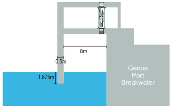
Figure 5.
Geometry of the OWC located on the offshore side of the breakwater that protects the port of Genoa (Italy).
For this real case, the horizontal grid step was , the number of grid cells along the vertical direction was , and the time step was , which guaranteed a Courant–Levy–Fredericks number of less than . The contribution to the energy production of every class of prevailing waves with a frequency of occurrence greater than (shown in Table 1) was calculated by a numerical simulation. At the end of every simulation, the mean mechanical power absorbed from those waves (per unit of length of the wavefront) was multiplied by its annual frequency of occurrence and by the length of the breakwater. The sum of every contribution gave the mean annual energy production.
By using the results of the numerical simulations carried out by the proposed model, the mean annual energy production that can be extracted from the waves at the Genoa port is equal to . This value is equivalent to the annual energy production of the wind park of Scampitella (AV), in southern Italy, which consists of 32 wind turbines with nominal power of each.
For this case study, the dimensions of the OWC and the significant wave height and peak period of the input irregular waves were significantly greater than those used in the laboratory tests. In such conditions, the air compressibility is no longer negligible. In order to quantify the difference in the numerical results obtained by considering or neglecting the air compressibility, all the numerical simulations for this case study were repeated by using a simplified pneumatic model, in which the air was assumed to be incompressible (incompressible air model). By adopting this simplification, the estimation of the mean annual energy production that can be extracted from waves at the Genoa port was , which was 8.56% higher than that obtained by the proposed model. An explanation of this overestimation may be that in the Genoa port case study, the pressure oscillations in the air chamber that were calculated by the incompressible air model were, on average, larger than those calculated by the compressible air model. In fact, by considering the air as incompressible, every variation per unit time of the volume of water inside the chamber (due to wave motion) caused an equivalent and simultaneous increase in the air flow through the turbine, which corresponded to a pressure variation inside the chamber with respect to the atmospheric one. In reality, the rapid variations in the water volume in the chamber due to wave motion can produce compressions or expansions of the air volume that hinder its movement and reduce the air flow through the turbine and the pressure variations inside the chamber (with a consequent decrease in the power absorbed by the OWC). The proposed compressible air model takes into account this effect and, for the same incident waves, produces pressure oscillations in the chamber that are, on average, smaller than those obtained by the air incompressible model.
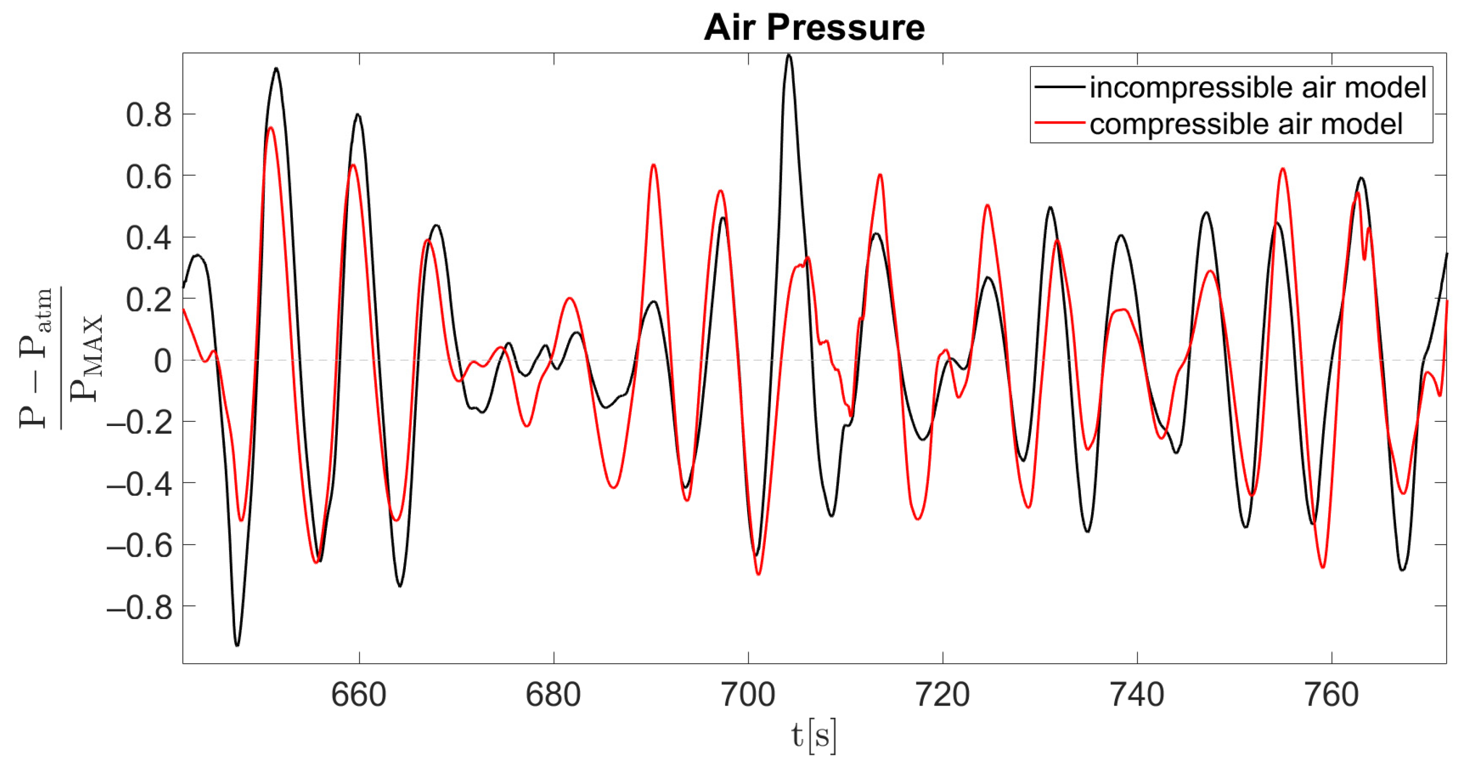
An example of these differences in pressure values inside the chamber is shown in Figure 6, which compares the time evolution of the air pressure in the chamber obtained by both the compressible and incompressible air models during the numerical simulations of the interaction between the OWC and irregular waves with a significant wave height of and a peak period of . For the sake of clarity, the pressure values shown in Figure 6 were non-dimensionalized by dividing them by the maximum pressure value found during the simulation (). In this figure, it is possible to see that higher pressure peaks (in absolute values) were obtained by the incompressible air model and that the maximum differences between the two models were almost 40%. The graph also shows that, during the numerical simulations, the absolute value of the pressure calculated by the incompressible air model was not always higher than the one calculated by the compressible air model. The presence of time intervals in which the opposite result takes places explains why the resulting mean annual energy obtained by the incompressible air model was only 8.56% higher than that calculated by the compressible air model.
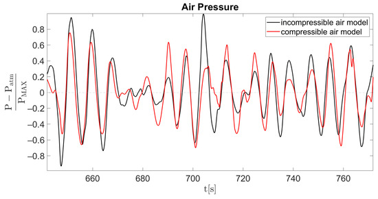
Figure 6.
Genoa port case study. Time evolution of non-dimensional air pressure inside the OWC chamber. Numerical results obtained by the compressible air model (red line) and incompressible air model (black line). ; ; .
3.2.2. Performance of an OWC Subjected to Breaking Waves (Paola Coast)
In this section, we present the results of the numerical simulations of the interaction between the prevailing waves and an OWC located on the offshore sides of a T-groin that protects the cost of Paola, in the southern Italy. The main difference with the previous real case is that the T-groin head is located within the surf zone, where the water depth is about 3 m, and most of the incident waves are breaking waves.
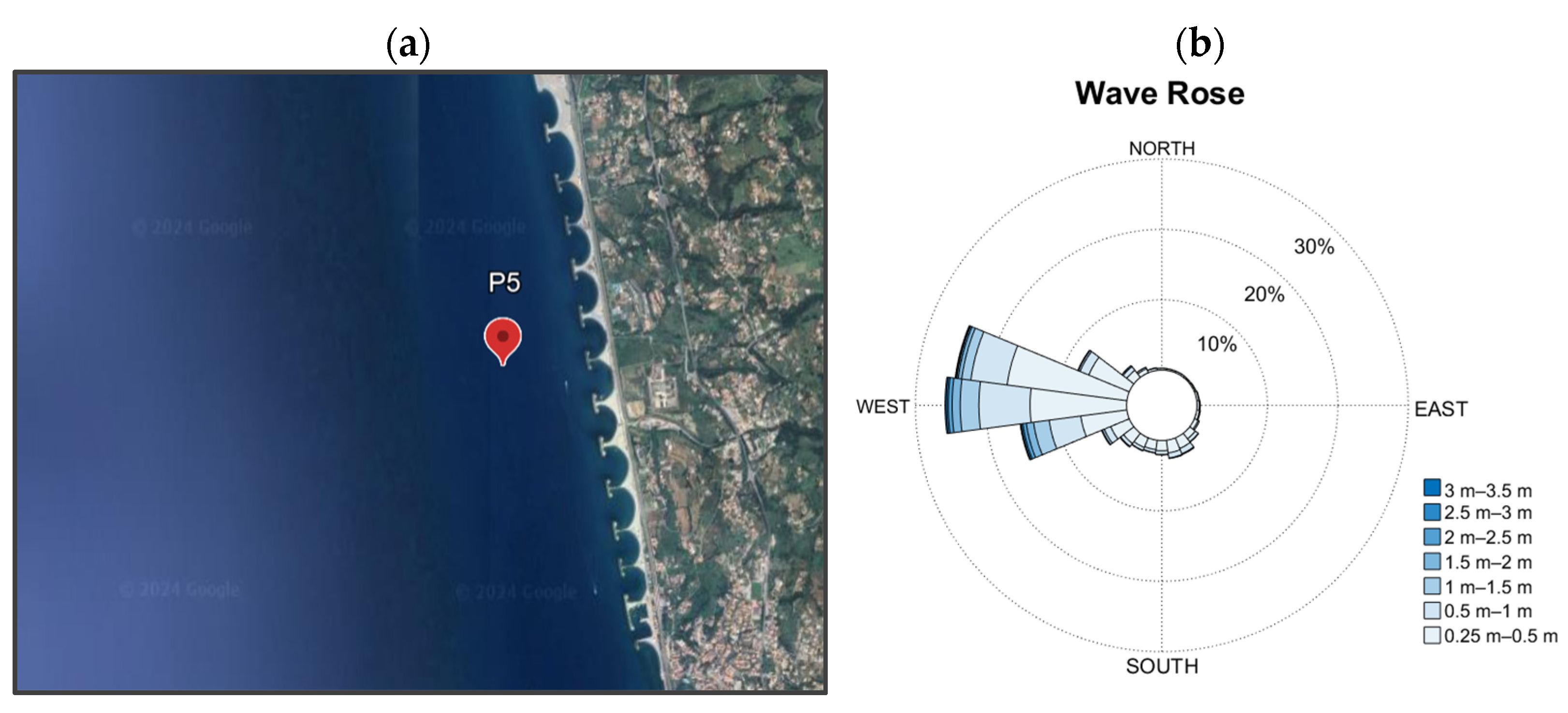
In order to statistically characterize the prevailing waves, we used the ERA5 reanalysis wave data at a point offshore the coast of Paola (point P5 in Figure 7a). The above point, about 500 m from the coast, was the starting point of the numerical simulations carried out by the proposed model. The waves characteristics of point P5 are shown in the polar diagram of Figure 7b and are listed in Table 2, where we highlight the data used to build the JONSWAP spectra of the irregular waves used as the input data of the numerical simulations.
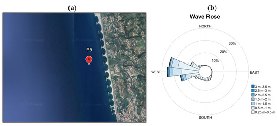
Figure 7.
(a) Coast of Paola and location of point P5. (b) Wave rose diagram of mean annual significant wave heights at point P5.
Table 2.
Mean annual wave characteristics of point P5, off the coast of Paola. Angle of direction of origin of the waves (significant wave height (), mean wave period (numbers inside the rectangles), and frequency of occurrence of every triplet (gray scale).
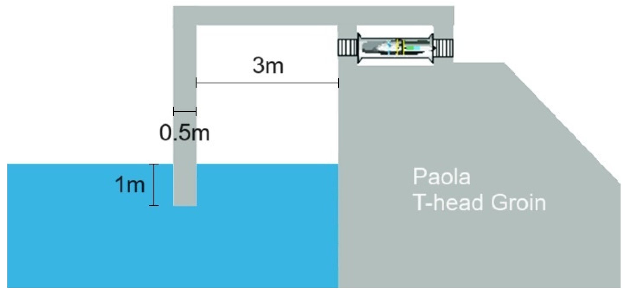
For this case study, the chosen waves were those coming from the sector with a frequency of occurrence greater than and a significant wave height of . The OWC was located on the offshore side of the head of the T-groin, had a chamber length equal to 3, and had a front wall draught equal to (Figure 8).

Figure 8.
Geometry of the OWC located on the offshore side of the T-groin that protects the coast of Paola (Italy).
The horizontal grid step was , the number of grid cells along the vertical direction was , and the time step was , which guaranteed a Courant–Levy–Fredericks number of less than . By considering the existing T-groins, each with a long head, the overall length of the barriers that can be equipped with an OWC is about . For this site, the results of the numerical simulations carried out by the proposed model gave an estimation of the mean annual energy production equal to .
As in the previous real case, the dimensions of the OWC and the characteristics of the simulated incoming waves were significantly greater than those used in the laboratory experiments and, therefore, the air compressibility was not negligible. Furthermore, differently from the previous case, most of the incoming waves were breaking waves that were characterized by steep wave fronts.
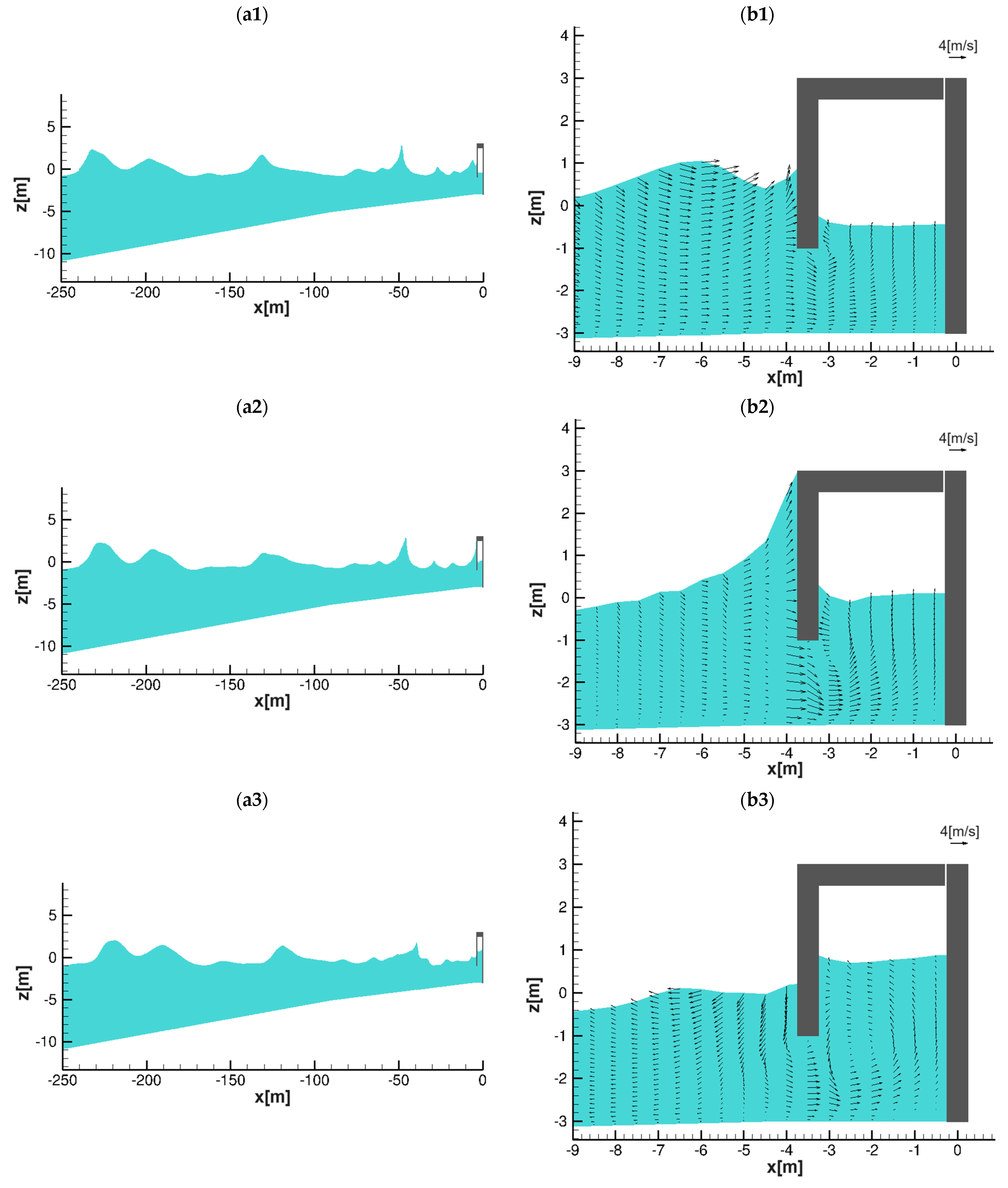
Figure 9 show a sequence of instantaneous wave fields and flow velocities obtained by the proposed model during the numerical simulations of the interaction between the OWC and irregular waves with a significant wave height of and a peak period of . As can be seen in the left images in Figure 9, the wave front significantly steepened and broke before reaching the OWC chamber. Consequently, the interaction of the short crest phase with the OWC was characterized by a rapid and significant increase in the water level within the chamber that was followed by its rapid decrease, while the subsequent longer trough phase was characterized by small water level variations (right images in Figure 9). The resulting pressure variations within the chamber are shown in Figure 10, where the numerical results obtained by the compressible air model are compared with those obtained by the incompressible air model.
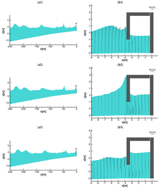
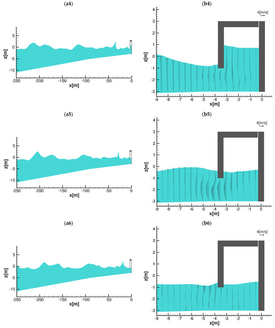
Figure 9.
Coast of Paola case. Interaction between OWC and irregular waves with significant wave height of and peak period of . Sequence of instantaneous wave fields (a1–a6) and detailed view of flow velocities (b1–b6).
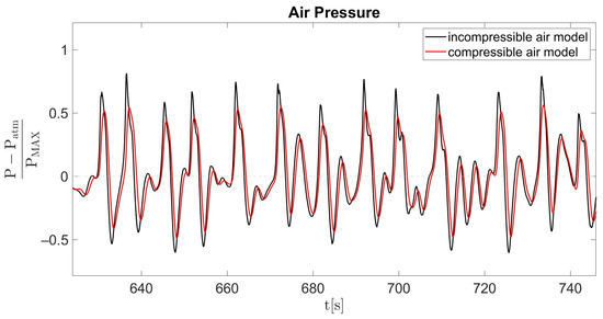
Figure 10.
Paola coast case study. Time evolution of non-dimensional air pressure inside the OWC chamber. Numerical results obtained by the compressible air model (red line) and incompressible air model (blue line).; ; .
Figure 10 shows that, differently from what happened in the case of non-breaking waves (Figure 6), in this case, the pressure oscillations calculated by the incompressible air model were systematically larger than those calculated by the compressible air model. By repeating all the numerical simulations of this real case carried out by the incompressible air model, we obtained a mean annual energy production equal to , which is greater than that obtained by the compressible air model. This overestimation was because the incompressible air model does not take into account the compression and expansion of the air volume within the OWC chamber produced by the rapid variations in the water level during the interaction between the OWC and the steep breaking wave fronts. Consequently, with this simplified pneumatic model, every water level oscillation directly produces an air flux through the turbine and overestimates the energy production.
4. Conclusions
A numerical study on the performances of an OWC subjected to non-breaking and breaking waves is presented in this paper. The potential mean annual energy production by OWCs in two Italian costal sites was evaluated. The numerical simulations were carried out both by the proposed numerical model and by a simplified pneumatic model usually adopted in the literature, in which the air within the OWC chamber is considered incompressible. The comparison between the numerical results demonstrate that the effects of the air compressibility can be considered negligible only in numerical simulations of the performances of reduced-scale OWC devices, such as those used in laboratory experiments. In such conditions, the numerical results obtained by the simplified pneumatic model and by the proposed one are almost coincident and are in good agreement with experimental data. On the contrary, the numerical simulations of the OWC performances carried out at a real scale (where the dimensions of the chamber and the wave characteristics are about one order of magnitude larger) show that in such conditions, the effect of the air compressibility within the chamber significantly reduces the ability of the OWC to extract energy from waves. In both the presented real case applications, the simplified pneumatic model (in which the air is assumed incompressible) gave an estimation of the OWC mean annual energy production that was systematically overestimated with respect to that obtained by the proposed compressible air model. Furthermore, the numerical results show that the effect of the air compressibility is more significant in the case of a real-scale OWC located in the surf zone, where it interacts with breaking waves. For this real case, the evaluation of the energy production obtained by the simplified pneumatic model was overestimated by about 31%.
Author Contributions
Conceptualization, G.C. and F.B.; methodology, G.C., F.B. and M.S.; validation, F.B. All authors have read and agreed to the published version of the manuscript.
Funding
This research received no external funding.
Institutional Review Board Statement
Not applicable.
Informed Consent Statement
Not applicable.
Data Availability Statement
The data presented in this study are available on request from the corresponding author due to privacy.
Conflicts of Interest
The authors declare no conflicts of interest.
References
- Falcão, A.F.O. Overview on Oscillating Water Column Devices. Mater. Res. Proc. 2022, 20, 1–9. [Google Scholar] [CrossRef]
- Falcão, A.F.O.; Henriques, J.C.C.; Gato, L.M.C. Self-rectifying air turbines for wave energy conversion: A comparative analysis. Renew. Sustain. Energy Rev. 2018, 91, 1231–1241. [Google Scholar] [CrossRef]
- Morris-Thomas, M.T.; Irvin, R.J.; Thiagarajan, K.P. An investigation into the hydrodynamic efficiency of an oscillating water column. J. Offshore Mech. Arct. Eng. 2007, 129, 273–278. [Google Scholar] [CrossRef]
- Ning, D.Z.; Wang, R.Q.; Zou, Q.P.; Teng, B. An experimental investigation of hydrodynamics of a fixed OWC Wave Energy Converter. Appl. Energy 2016, 168, 636–648. [Google Scholar] [CrossRef]
- Romolo, A.; Timpano, B.; Laface, V.; Fiamma, V.; Arena, F. Experimental Investigation of Wave Loads on U-OWC Breakwater. J. Mar. Sci. Eng. 2023, 11, 19. [Google Scholar] [CrossRef]
- Ning, D.; Shi, J.; Zou, Q.; Teng, B. Investigation of hydrodynamic performance of an OWC (oscillating water column) wave energy device using a fully nonlinear HOBEM (higher-order boundary element method). Energy 2015, 83, 177–188. [Google Scholar] [CrossRef]
- Kim, J.S.; Nam, B.W.; Park, S.; Kim, K.H.; Shin, S.H.; Hong, K. Numerical investigation on hydrodynamic energy conversion performance of breakwater-integrated oscillating water column-wave energy converters. Ocean Eng. 2022, 253, 111287. [Google Scholar] [CrossRef]
- Koo, W.; Kim, M. Nonlinear time-domain simulation of a land-based oscillating water column. J. Waterw. Port Coast. Ocean Eng. 2010, 136, 276–285. [Google Scholar] [CrossRef]
- Wan, C.; Yang, C.; Bai, X.; Bi, C.; Chen, H.; Li, M.; Jin, Y.; Zhao, L. Numerical investigation on the hydrodynamics of a hybrid OWC wave energy converter combining a floating buoy. Ocean Eng. 2023, 281, 114818. [Google Scholar] [CrossRef]
- Ma, G.; Shi, F.; Kirby, J. Shock-capturing non-hydrostatic model for fully dispersive surface wave processes. Ocean Model. 2012, 43, 22–35. [Google Scholar] [CrossRef]
- Derakhti, M.; Kirby, J.T.; Shi, F.; Ma, G. Wave breaking in the surf zone and deep-water in a non-hydrostatic RANS model. Part 1: Organized wave motions. Ocean Model. 2016, 107, 125–138. [Google Scholar] [CrossRef]
- Cannata, G.; Petrelli, C.; Barsi, L.; Gallerano, F. Numerical integration of the contravariant integral form of the Navier-Stokes equations in time-dependent curvilinear coordinate system for three-dimensional free surface flows. Contin. Mech. Thermodyn. 2019, 31, 491–519. [Google Scholar] [CrossRef]
- Cannata, G.; Simone, M.; Gallerano, F. Numerical Investigation into the Performance of an OWC Device under Regular and Irregular Waves. J. Mar. Sci. Eng. 2023, 11, 735. [Google Scholar] [CrossRef]
- Torres, F.R.; Teixeira, P.R.F.; Didier, E. Study of the turbine power output of an oscillating water column device by using a hydrodynamic—Aerodynamic coupled model. Ocean Eng. 2016, 125, 147–154. [Google Scholar] [CrossRef]
- Teixeira, P.R.F.; Davyt, D.P.; Didier, E.; Ramalhais, R. Numerical simulation of an oscillating water column device using a code based on Navier.Stokes equations. Energy 2013, 61, 513–530. [Google Scholar] [CrossRef]
- Josset, C.; Clément, A.H. A time-domain numerical simulator for oscillating water column wave power plants. Renew. Energy 2007, 32, 1379–1402. [Google Scholar] [CrossRef]
- Cannata, G.; Palleschi, F.; Iele, B.; Gallerano, F. A Wave-Targeted Essentially Non-Oscillatory 3D Shock-Capturing Scheme for Breaking Wave Simulation. J. Mar. Sci. Eng. 2022, 10, 810. [Google Scholar] [CrossRef]
- Moran, M.J.; Shapiro, H.N. Fundamentals of Engineering Thermodynamics, 5th ed.; Wiley: Chichester, UK, 2006; pp. 128–131. [Google Scholar]
- Booij, N.; Holthuijsen, L.H.; Ris, R.C. The “SWAN” wave model for shallow water. Coast. Eng. 1996, 25, 668–676. [Google Scholar] [CrossRef]


Disclaimer/Publisher’s Note: The statements, opinions and data contained in all publications are solely those of the individual author(s) and contributor(s) and not of MDPI and/or the editor(s). MDPI and/or the editor(s) disclaim responsibility for any injury to people or property resulting from any ideas, methods, instructions or products referred to in the content. |
© 2024 by the authors. Licensee MDPI, Basel, Switzerland. This article is an open access article distributed under the terms and conditions of the Creative Commons Attribution (CC BY) license (https://creativecommons.org/licenses/by/4.0/).