Investigations into Motion Responses of Suspended Submersible in Internal Solitary Wave Field

Abstract

When the underwater submersible encounters an internal solitary wave (ISW), its loadings and motions are significantly disturbed. To investigate the interaction mechanism between the suspended submersible and the ISW, a three-dimensional ISW–submersible-interaction numerical model was established, based on the computational fluid dynamics (CFD) method. The generation and propagation of the ISW was simulated in a two-layer fluid numerical wave tank, according to the eKdV theory. The standard operation equation of the submersible was introduced to simulate the six degree of freedom (6DoF) motions of the submersible combined with the overset dynamic mesh method. The motion simulation method was effectively validated by comparing it with published experimental results on the motion responses of a slender body under the ISW. Based on the constructed numerical model, the dynamic mechanisms between the suspended submersible and the ISW were studied, and the effects of the initial submerged depths and the ISW amplitudes on the dynamic responses of the submersible were revealed. According to the numerical results, the motions of the submersible have been significantly determined by its initial submerged depths. The submersible located above the ISW interface has a significant motion along the propagation direction of the ISW and its motion trajectory resembles a counterclockwise semi ellipse. The motion of the submersible located below the ISW interface follows the trace of the lower layer of fluid, which presents as an unclosed clockwise ellipse. The corresponding motions of the submersible would be increased with the increase in the ISW amplitudes.

1. Introduction

An internal solitary wave (ISW) is a kind of nonlinear fluctuation that frequently occurs in the stratified ocean. Due to the small difference in vertical density, the hydrostatic recovery forces of the ISW are much less than that of the free surface wave. Even a small disturbance in the stratified ocean can cause a large amplitude nonlinear internal wave [1,2]. Moreover, due to the balance between dispersion and the nonlinearity effect, the ISW can propagate over several hundred kilometers with a stable wave shape and propagating speed. It carries huge energy in the process of propagation and causes extremely strong underwater shear currents [3,4,5]. Under the action of the huge ISW currents, the loadings and motions of the marine structures may be heavily disturbed, especially for the submerged structure, which is affected by the ISW fluid field directly. In recent years, the reports of the underwater submersible crashing or even sinking while encountering the ISW are not rare [6,7,8]. Therefore, it is necessary and urgent to carry out the investigations into the interaction mechanisms between the ISW fluid field and the movable submersible to improve the safety and maneuverability of the submersible while encountering the ISW.

In order to prevent or weaken the damage caused by the ISW to the marine structures, over the years, many scholars have carried out experimental investigations into the interaction mechanism between the submerged or floating structures and the ISW. For the floating structures, Chen et al. [9,10] performed experimental research on the fixed semi-submersible platform under the ISW environment and measured the ISW loadings on the platform. Cui et al. [11] conducted experimental studies on the moored structure and obtained the motion responses and mooring tensions of the floating structure under the action of the ISW. Moreover, Sara et al. [12] conducted a laboratory experiment to simulate the motion responses of the SPAR wind turbine. For the submerged structure, Wang et al. [13,14] carried out experimental studies on the interaction effect between the ISW and a fixed underwater slender body in the stratified flume and revealed the relationships between the fixed structure and the ISW fluid field. Cui et al. [15,16] recorded the real-time motion responses of the underwater structure under the ISW through the experimental method, and the influences of the amplitude of the ISW and fluid stratification ratios on the motion responses were discussed. However, the model experiments are constrained by the scale effects. In the above-mentioned experiments, the scales of the characteristic structure were intentionally enlarged in order to better measure the loadings or capture the motions of the structure, which may result in some difficulties in converting the experimental results to the realistic physical background. Additionally, there are few experimental studies on the complex structure model, and more attention is drawn to the simple structures such as cylinders or spheres.

Considering the scale effect and high costs of the experimental method, the theoretical analysis method has gradually become an effective way to investigate the interaction mechanism between the ISW and structures. Cai [17,18,19] proposed a new method based on the ISW theory and Morison equations to calculate the ISW loadings on the simple slender cylindrical structure. Based on the above method, some scholars [20,21,22] simulated the motions of the structures while encountering the ISW by introducing the 6DOF motion equations of the rigid body. Moreover, some scholars [23,24] investigated the interaction effect between the floating structure and the ISW based on the potential theory combined with ISW equations. Although most previous investigations of the motion simulations using a mathematical model were convenient and efficient, they cannot consider the dynamic interaction effects between the ISW fluid field and the structure. That is, the theoretical analysis method ignores the interference of the structures on the fluid field and also cannot capture the generation and propagation characteristics of the ISW.

The CFD method has a lower computational efficiency, and its calculation accuracy is limited by the quality of grid. However, the CFD method can fully consider the dynamic two-way interaction effects between the structure and the fluid field and would not be affected by the scale effect. Recently, the CFD method has been widely used to investigate the interaction mechanism between the ISW and the structures. Many scholars [25,26,27] established the numerical model to investigate the FSI (fluid–structure interaction) effect between the ISW and the fixed structure and obtained the loading history of the structure. Subsequently, some scholars [28,29,30] have studied the interaction characteristics between the ISW and the movable structure, and obtained the motion responses of the structure by applying the 6DOF calculation module of CFD software directly. However, the motion responses of the structure may be overestimated, while the underwater stability of the structure is ignored, especially in the pitch direction.

Extensive investigations have been carried out to reveal the interaction effects between the underwater structure and the ISW. However, most previous investigations focus on the ISW loading characteristics on a fixed structure. The investigation into the motion characteristics of the submersible under the ISW environment is still scarce. In order to further investigate the ISW–structure dynamic interaction effects, a time-domain numerical model is proposed, based on the secondary development of CFD software in this paper. The numerical theories involved are introduced in Section 2, and the modeling and validating of the numerical model are introduced in Section 3. In Section 4, the effects of the initial submerged depths of the submersible and the amplitudes of the ISW on the motion responses of the submersible are addressed according to the numerical results. Finally, the conclusions are drawn in Section 5.

2. Theory and Numerics

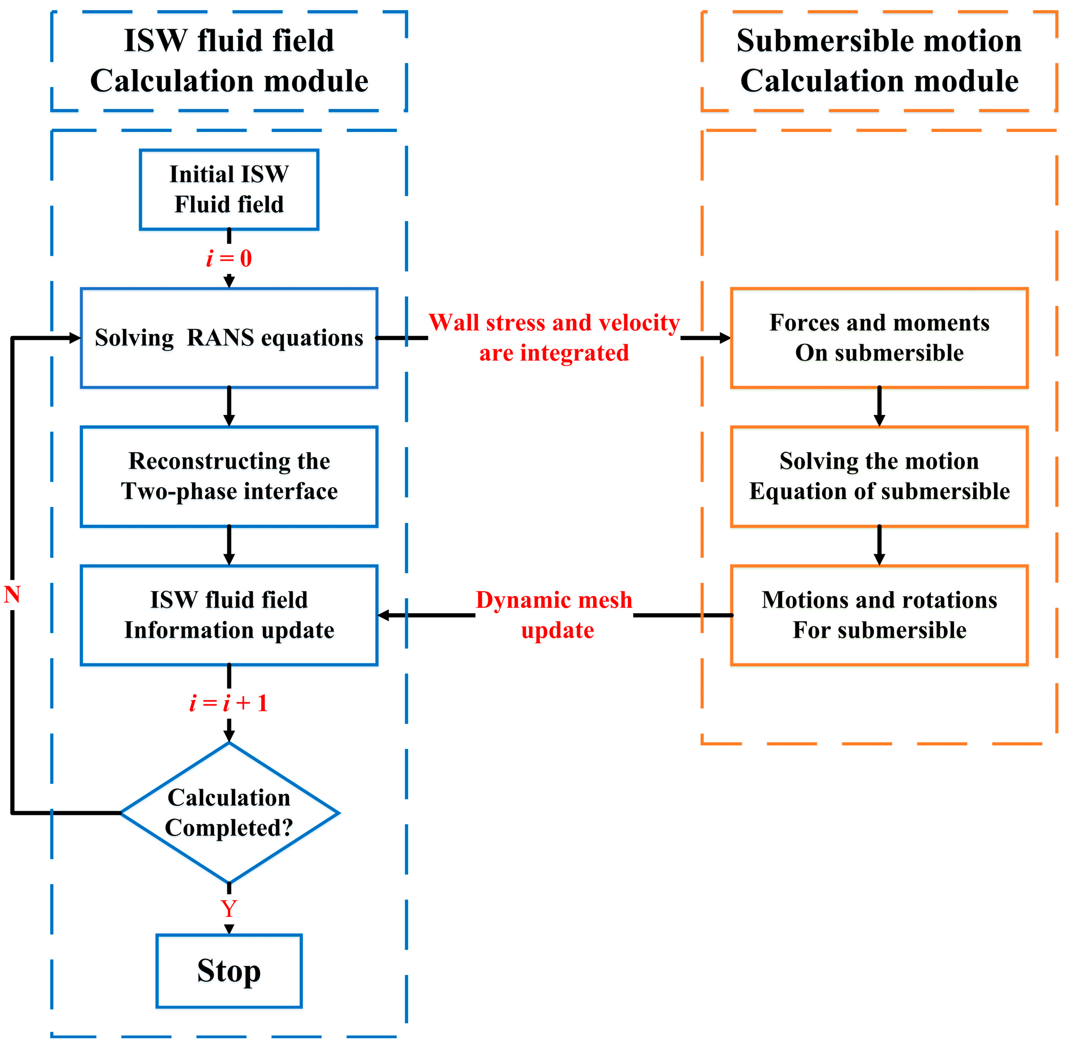
2.1. Basis Equations for Fluid–Structure Interaction

To simulate the motion properties of the movable submersible in the ISW fluid field, therefore, the fluids are treated as incompressible and viscous, to calculate the driving forces acting on the submersible more accurately. The governing equations of the ISW fluid field are the mass continuity equation and the Reynolds-averaged Navier–Stokes (RANS) equations [31]. They can be written as follows:

$$\frac{\mathsf{\partial }\overline{u_i}}{\mathsf{\partial }{x}_i}=0,$$

(1)

$$\frac{\mathsf{\partial }\overline{u_i}}{\mathsf{\partial }t}+\sum _j\overline{u_j}\frac{\mathsf{\partial }\overline{u_i}}{\mathsf{\partial }{x}_j}=-\frac{1}{\rho }\frac{\mathsf{\partial }P}{\mathsf{\partial }{x}_i}+F_i+v\sum _j\frac{{\mathsf{\partial }}^2\overline{u_i}}{\mathsf{\partial }{x}_i^2}-\sum _j\frac{\mathsf{\partial }\overline{u_i^{\prime }{u}_j^{\prime }}}{\mathsf{\partial }{x}_j},$$

(2)

where ${\overline{u}}_i$ is the time-average velocity; $u_i^{\prime }$ represents the fluctuation velocity; $F_i$ is the mass force; $P$ is the pressure; $\rho$ is the fluid density; and $\nu$ is the fluid kinematic viscosity. The above fluid-governing equations are numerically solved by the finite volume method (FVM). The turbulent viscosity of the above governing equations $\nu$ is solved by the RNG k-ε two-equation closed model [32]. The coupled algorithm is applied to solve the pressure–velocity coupling term. Considering the influences of gravity, the body-force weighted method is used for pressure interpolation. The velocity gradient on the left inlet side is solved by the least squares cell-based method.

In order to accurately describe the motion responses and loading characteristics of the suspended submersible under the action of the ISW, here, the two coordinate systems are defined which contained the Earth-fixed coordinate system E-xyz and the moving coordinate system O-x₀y₀z₀ [33]. As shown in Figure 1, the fixed coordinate system is introduced to describe the translational movement of the submersible while its coordinate system origin called E is exactly right on the geometric center of the interface of the two-phase fluid at the velocity entrance. The moving coordinate system is established to describe the hydrodynamic characteristics and rotational movements of the submersible while its coordinate-system origin called O coincides with the center of gravity of the submersible and always moves with the submersible.

In this paper, the standard operation equations of the submersible [34] are introduced to describe the ISW-driven motions of the submersible, and the underwater stability of the submersible is fully considered:

$$\begin{array}{l}m(\frac{\mathsf{\partial }u}{\mathsf{\partial }t}+qw-rv)=F_x\\ m(\frac{\mathsf{\partial }v}{\mathsf{\partial }t}+ru-pw)=F_y\\ m(\frac{\mathsf{\partial }w}{\mathsf{\partial }t}+pv-qu)=F_z\\ I_{xx}\frac{\mathsf{\partial }p}{\mathsf{\partial }t}+(I_{zz}-I_{yy})qr=M_x+N_x\\ I_{yy}\frac{\mathsf{\partial }q}{\mathsf{\partial }t}+(I_{xx}-I_{zz})rp=M_y+N_y\\ I_{zz}\frac{\mathsf{\partial }r}{\mathsf{\partial }t}+(I_{yy}-I_{xx})pq=M_z+N_z\end{array}$$

(3)

where $m$ is the mass of the submersible, $I_{xx}$,$I_{yy}$,$I_{zz}$ are the rotational inertia of the submersible, $u$, $v$, $w$ are the translation velocities of the submersible, $p$, $q$, $r$ are the angular velocities of the submersible relative to the moving coordinate system, and $F_x$,$F_y$,$F_z$ and $M_x$,$M_y$,$M_z$ are the fluid field forces and torques applied on the wet surface of the submersible by the fluid field, which are obtained by solving the discretized RANS equations on Fluent. As seen in the schematic drawing in Figure 2,$N_x$,$N_y$,$N_z$ are the recovery torques of the submersible, derived from the stability of the submersible itself:

$$\left(N_x,N_y,N_z\right)=mg\Delta h\left(-\sin {\theta }_x,-\sin {\theta }_y,0\right),$$

(4)

where ${\theta }_x$,${\theta }_y$ are the turning angles of the submersible in the roll and pitch directions, respectively, and Δh is the height difference between the center of gravity B and the center of buoyancy G.

In order to simulate the two-way FSI process, the interface between the ISW fluid field and the movable submersible is established based on the secondary development of Fluent to achieve the numerical information exchange [35]. The numerical implementation method of the FSI interface is to write the user-defined function (UDF) combined with the overset dynamic mesh method. The specific fluid–structure interaction process is shown as follows, in Figure 3: The generation and propagation of the ISW is simulated in the numerical wave tank by enforcing the internal wave flow conditions on the inlet boundary based on the solution of the ISW equations, and dispersed RANS equations are solved to obtain the hydrodynamic loadings on the submersible in Fluent. The volume of fluid (VOF) method is introduced to capture the generation and evolution of the ISW interface [36]. Then the motions of the submersible can be calculated by introducing the hydrodynamic loadings acting on the wet surface into the standard motion equation of the submersible; thus, the effect of the fluid field on the structure can be considered. Based on the overset dynamic mesh method, the wall boundary of the submersible is updated on the fluid field according to the numerical calculated results to consider the influences of the motions of the structure on the fluid field. The aforementioned process is repeated until the all fluid–structure calculations are complete.

2.2. Theory of Internal Solitary Wave

To simplify the numerical solving process below, the actual continuous-layer density structure of the ocean can be assumed as a fluid with two uniform-density layer systems [37]. As shown in Figure 4, the densities of the upper and lower layer are ${\rho }_1$ and ${\rho }_2$, respectively. The depths of the upper and lower layer are $h_1$ and $h_2$, respectively. The fluid interface between the upper- and lower-fluid layers is treated as the pycnocline. The top boundary side follows the rigid-lid assumption, while the bottom boundary is regarded as a no-slip wall.

There are multifarious numerical theories to describe the ISW [38,39,40,41,42], and different equations are suitable to simulate the generation of the ISW for different depth ratios $h_1/h_2$ and different amplitudes ${\xi }_0$. The eKdV equation [43] is suited to describe the ISW with middle nonlinear amplitude, and this paper employs the eKdV equation to initialize the ISW fluid field. The interface displacement of the ISW can be expressed as follows:

$$\begin{array}{l}\frac{\mathsf{\partial }\zeta }{\mathsf{\partial }t}+c_0\frac{\mathsf{\partial }\zeta }{\mathsf{\partial }x}+c_1\zeta \frac{\mathsf{\partial }\zeta }{\mathsf{\partial }x}+c_2\frac{{\mathsf{\partial }}^3\zeta }{\mathsf{\partial }{x}^3}+c_3{\zeta }^2\frac{\mathsf{\partial }\zeta }{\mathsf{\partial }x}=0,\\ c_0^2=g{h}_1{h}_2\left({\rho }_2-{\rho }_1\right)/\left({\rho }_1{h}_2+{\rho }_2{h}_1\right),\\ c_1=-3c_0\left({\rho }_1{h}_2^2-{\rho }_2{h}_1^2\right)/\left[2\left({\rho }_1{h}_1{h}_2^2+{\rho }_2{h}_1^2{h}_2\right)\right],\\ c_2=c_0\left({\rho }_2{h}_1{h}_2^2+{\rho }_1{h}_1^2{h}_2\right)/\left[6\left({\rho }_1{h}_2+{\rho }_2{h}_1\right)\right],\\ c_3=\frac{3c_0}{h_1^2{h}_2^2}\left(\frac{7}{8}{\left(\frac{{\rho }_1{h}_2^2-{\rho }_2{h}_1^2}{{\rho }_1{h}_2+{\rho }_2{h}_1}\right)}^2-\frac{{\rho }_1{h}_2^3+{\rho }_2{h}_1^3}{{\rho }_1{h}_2+{\rho }_2{h}_1}\right),\end{array}$$

(5)

where $\xi$ denotes the wave profile of the ISW, the analytical solution of $\xi (x, t)$ is

$$\begin{array}{l}\zeta (x,t)={\zeta }_0/\left[B+(1-B){\cosh }^2\left(\left(x-c_{eKdV}t\right)/{\lambda }_{eKdV}\right)\right],\\ B=-c_3{\zeta }_0/\left(2c_1+c_3{\zeta }_0\right),\end{array}$$

(6)

its phase velocity $c_{eKdV}$ and characteristic wave length ${\lambda }_{eKdV}$ are

$$c_{eKdV}=c_0+{\zeta }_0\left(c_1+c_3{\zeta }_0/2\right)/3,$$

(7)

$${\lambda }_{eKdV}=\sqrt{12c_2/\left[\left(c_1+c_3{\zeta }_0/2\right){\zeta }_0\right]},$$

(8)

Numerical simulation of the ISW is carried out by solving the eKdV equation and enforcing the velocity distribution condition on the inlet flow boundary. The upper-layer and lower-layer velocity can be derived from the ISW profiles, respectively [44]. The induced velocities of the upper-layer and lower-layer fluid $u_1$ and $u_2$ are

$$u_i={(-1)}^i\frac{c_{eKdV}{\zeta }_0}{h_i}, \mathrm{where} i=1,2$$

(9)

3. Modeling and Validations

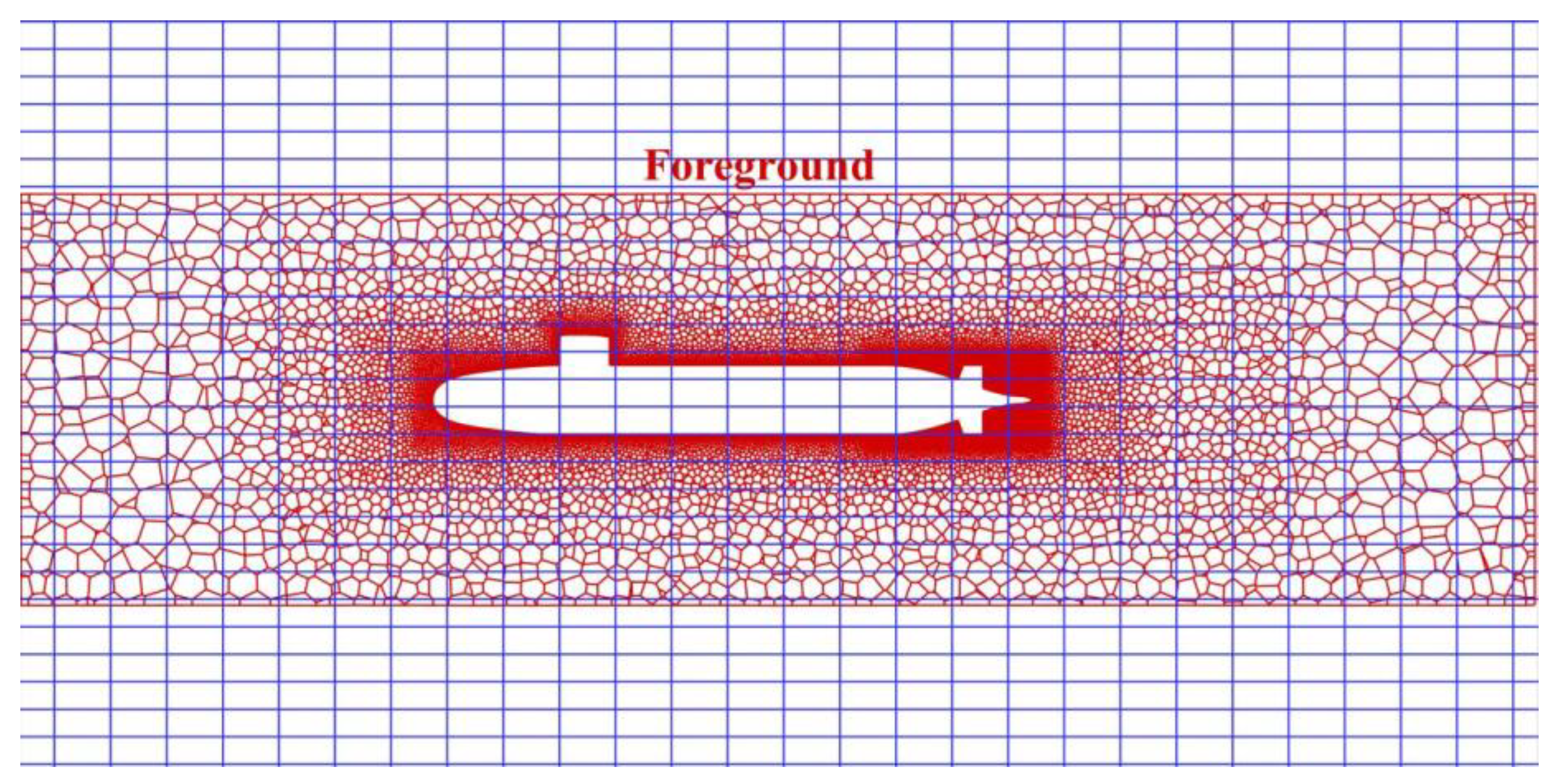
3.1. ISW Numerical Tank and Submersible Model

In this paper, the standard submersible model proposed by the Defense Advanced Research Projects Agency (DARPA), called Suboff [45,46], with a scale of 1:20 is introduced to investigate the fluid–structure interaction effect between the ISW fluid field and the movable submersible. The total length and the maximum diameter of the submersible model are $L_{pp}=4.356 \mathrm{m}$ and $D=0.508 \mathrm{m}$, respectively. The volume of displacement of the submersible is $V=0.705 {\mathrm{m}}^3$ and the height difference between the gravity center G and the buoyancy center B is $\mathsf{\Delta }h=0.0162 \mathrm{m}$. The schematic diagram of the interaction of the numerical model is given in Figure 5. The length of the wave tank is $L=150 \mathrm{m}$, while its width and height are taken as $B=15 \mathrm{m}$ and $H=20 \mathrm{m}$, respectively. The head of the submersible is oriented toward the propagation direction of the ISW, and the initial location of the submersible is 50 m away from the velocity inlet boundary. According to the relevant papers [27,28,29,46,47,48], for the numerical wave-generation tank, the depths of the upper- and lower-fluid layers are $h_1=5 \mathrm{m}$ and $h_2=15 \mathrm{m}$, respectively, and the densities of the upper- and lower-fluid layers are ${\rho }_1=998 \mathrm{k}\mathrm{g}/{\mathrm{m}}^3$ and ${\rho }_2=1025 \mathrm{k}\mathrm{g}/{\mathrm{m}}^3$, respectively. The amplitude of the ISW is set as ${\xi }_0=-3 \mathrm{m}$. According to Equations (5)–(8), the length and period of the ISW are ${\lambda }_{eKdV}=19.94 \mathrm{m}$ and $T_{eKdV}=17.79 \mathrm{s}$, respectively, and its phase velocity is $c_{eKdV}=1.12 \mathrm{m}/\mathrm{s}$. It is also necessary to clarify that the constructed interaction numerical model in this paper meets the scale demanded of 1:20.

The initial submerged depth of the submersible called d is defined to describe the relative vertical distance between the initial position of the submersible and the ISW interface. At the initial moment, while the submersible is above the ISW interface, $d>0$; while the submersible is exactly at the center of the fluid interface, $d=0$; and while the submersible is below the fluid interface, $d<0$. In order to ensure that the submersible could be suspended in the fluid field stably, the density of the submersible body is modified to be consistent with that of the fluid field. The top side of the numerical tank is defined as the symmetrical boundary, according to the rigid-lid assumption. The left and right boundaries are allocated as the velocity inlet boundary and the pressure outlet boundary, respectively. The surface of the submersible and the bottom of the numerical wave tank are both defined as the wall boundary, while the front and back boundaries are both defined as the symmetrical boundary.

This paper aims to investigate the interaction effect between the movable submersible and the ISW fluid field. The overset dynamic mesh method is introduced to consider the large-amplitude motions of the suspended submersible, which can guarantee the nearby grids remaining free from distortion during the motion [49]. As Figure 6 shows, the whole component domain grid is divided into two parts: the foreground grid marked in red and the background grid marked in blue. The background region is meshed by the structured grid while the foreground region is meshed by the unstructured polyhedral grid. The foreground grid uses mesh refinement near the surface of the submersible, which can calculate the hydrodynamic loadings and motions of the submersible more precisely. In order to capture the ISW surface more accurately, the background grid also partially uses mesh refinement near the ISW surface to make the local mesh size 0.2 m. Moreover, the foreground region is set as the dynamic mesh component to simulate the ISW-driven motions of the submersible while the background region is set as fixed. The overset interface is constructed to transfer the fluid field information between the movable structure and background fluid field through the method of interpolation. The overset mesh size should be approximately the same as the nearby background mesh size to ensure the quality of the interpolation.

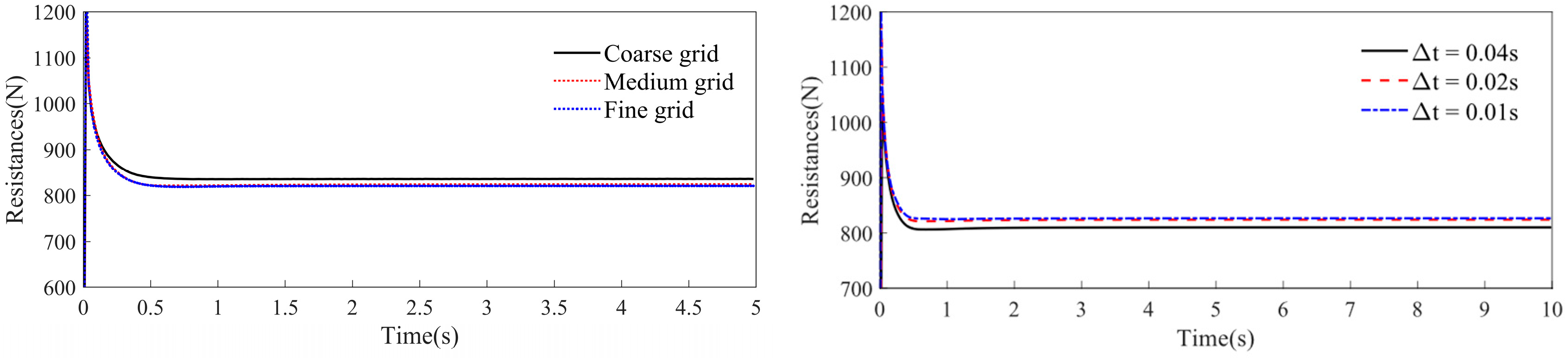
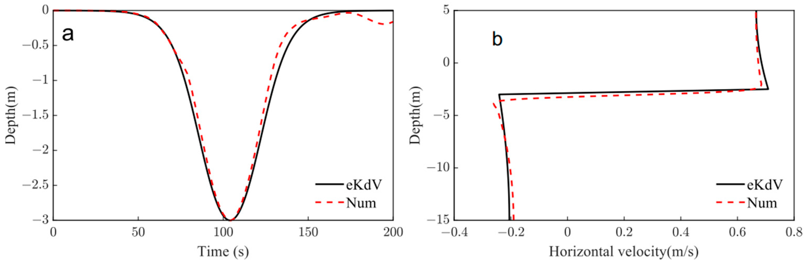
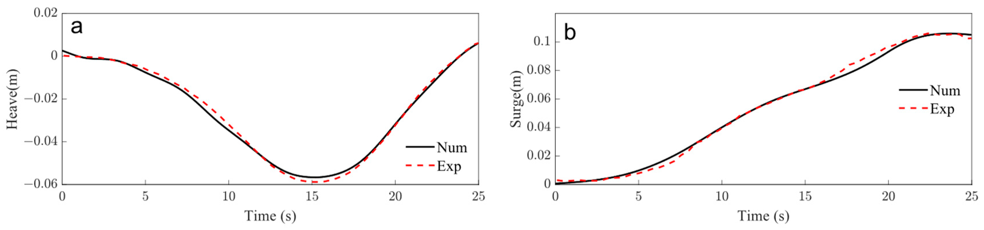
3.2. Numerical Validations

To test the grid and time-step independence of the conducted numerical model, three different foreground grid sizes (i.e., 0.04, 0.02, and 0.01 m) and three different time steps (i.e., 0.04, 0.02, and 0.01 s) are adopted to simulate the resistances of the submersible under the current at a velocity of 17.75 kn. As shown in Figure 7 below, the results indicate that the foreground grid size of 0.02 m and the time step of 0.02 s is accurate enough for the further simulations in Section 4.

Table 1. Relative error between the numerical and experimental resistances of Suboff model.

Velocity (kn)	Numerical Resistances (N)	Experimental Resistances (N)	Relative Error (%)
10	282	284	−0.704
11.85	387	389	−0.514
13.92	526	527	−0.190
16	680	676	0.592
17.79	827	821	0.731

gives the comparison of the resistances of the submersible at different velocities obtained by the numerical method and the experimental method. The reference solution of the experimental result is from the towing tank experiment conducted by Liu and Huang in 1998 [46]. The relative error between the experimental results and the numerical results is less than 1%, and the numerical model can precisely calculate the loadings of the structure.

To validate the accuracy of the ISW generation method, we simulate the generation and propagation of the ISW and record the time history of the ISW interface and the vertical distribution of the horizontal velocity. As shown in Figure 8, good agreements are achieved by comparing the numerical result and theoretical solution of the eKdV equation. Moreover, in the last published article [29], the ISW field and loadings of the underwater structure were well validated by comparing them with the experimental data.

In order to further validate the reliability of the motion simulation of the underwater structure under the action of the ISW, the numerical simulation was conducted and compared with the experimental data of Cui et al. [14]. As shown in Figure 9, the length, width and height of the numerical tank are 15 m, 0.4 m and 0.5 m, respectively, and the depths of the upper- and lower-fluid layers are 0.15 m and 0.35 m, respectively. The density of the upper fluid and lower fluid are ${\rho }_1=998 \mathrm{k}\mathrm{g}/{\mathrm{m}}^3$ and ${\rho }_2=1015 \mathrm{k}\mathrm{g}/{\mathrm{m}}^3$, respectively, and the amplitude of ISW is ${\xi }_0=-6 \mathrm{c}\mathrm{m}$. The length and diameter of the underwater slender body structure are 29.8 cm and 8 cm, respectively. The slender body is placed at the center of the pycnocline, which is 5 m away from the wave-generation boundary. Figure 10 shows the comparison between the calculated motions and the experimental data. The numerical results are in good agreement with the experimental results, which illustrates the fact that the present numerical model is accurate enough to simulate the motions of the underwater structure in the ISW fluid field.

4. Results and Discussions

Due to the strong effect of the ISW fluid field, the motion trajectory of the submersible would be significantly disturbed and the submersible moves up and down during the whole process. In this section, the motion characteristics of the suspended submersible under the ISW is reported, and the influences of the initial submerged depth of the submersible $d$ and the wave amplitude of ISW ${\xi }_0$ on the interaction effects are fully discussed. In order to simplify the numerical case analysis below, the relevant physical quantities such as submerged depth and motions of the structure are converted to dimensionless form by the following expressions:

$$\begin{array}{l}{X}^{*}=\frac{X}{H},Y^{*}=\frac{Y}{H},Z^{*}=\frac{Z}{H}\\ {\zeta }_0^{*}=\frac{{\zeta }_0}{H},d^{*}=\frac{d}{H}\end{array}$$

(10)

The dimensionless variables are introduced with a mark *, and $X$, $Y$ and $Z$ indicate the surge, sway and heave motions of the submersible, respectively.

4.1. Dynamic Responses of the Suspended Submersible under ISW

In this section, the numerical simulation is conducted to explore the dynamic interaction characteristics of the submersible under the ISW fluid field. The suspended submersible is placed at the upper layer of fluid ($d^{*}=0.05$) and the amplitude of the ISW is set as ${\xi }_0^{*}=-0.15$, while other parameters are the same as in Section 3.1 and Section 3.2. Figure 11 gives the whole interaction process between the movable submersible and the ISW surface through the velocity-vector contours. It can be observed that the motions of the submersible are always dominated by the internal-wave fluid field. As the ISW surface propagates near or away from the submersible in the horizontal direction, the submersible moves down first and then moves up quickly.

Figure 12 gives the time history of the motion responses of the suspended submersible located at the upper layer of fluid ($d^{*}=0.05$). In order to describe the interaction process more conveniently, the whole interaction process is divided into three stages, according to the amplitude of the heave motion, which are marked as I, II, and III in Figure 12. The two adjacent stages are separated by vertical black dashed lines. In stage I (0 s–80 s), the ISW propagates forwards and gradually approaches the submersible; the submersible moves slowly, driven by the ISW fluid field. In stage II (80 s–140 s), the submersible dives to the maximum dropping depth under the action of the internal-wave fluid field, while the submersible moves quickly along in the direction of the ISW propagation. In stage III (140 s–200 s), the submersible quickly floats up to the initial suspended surface while the submersible moves to the positive amplitude first and then moves backwards for a short distance, in the horizontal direction.

In the horizontal direction, under the guidance of the ISW fluid field, the suspended submersible moves, and its moving speed changes with the relative horizontal distance to the ISW surface. While the submersible is far from the wave surface, the moving speed is relatively low. By contrast, while the ISW surface propagates to close to the submersible, the submersible will be strongly disturbed by the core fluid field, and its moving speed will increase significantly. Due to the high horizontal velocity of the ISW fluid field, the driven motion of the suspended submersible in the horizontal direction is most significant. Moreover, the propagation phase velocity of the ISW is much larger than the horizontal moving velocity of the submersible; the submersible stops moving and does not continue to follow the fluid field of the ISW after moving for a certain distance along the positive-propagation direction of the ISW.

In the vertical direction, at the first two stages, the ISW propagates forwards and gradually approaches the submersible. Under the action of the ISW fluid field near the right side of the wave surface, the submersible continues to dive, and its diving speed increases as the ISW surface approaches the submersible; Figure 11a–e show the diving process of the submersible. The submersible reaches its dropping amplitude at the end of stage II ($\mathrm{t}\mathrm{i}\mathrm{m}\mathrm{e}=140 \mathrm{s}$), as shown in Figure 11e, and at this time, the submersible is located just above the trough of the ISW. Therefore, the dropping amplitude of the submersible is less than the wave amplitude of the ISW. At stage III, as shown in Figure 11f–h, the submersible quickly moves up and returns to the initial suspended surface under the action of the fluid field near the left wave surface.

In the pitch direction, the pitch angle of the submersible ${\theta }_y$ has hardly changed at the first two stages, and only generates a small angle, which is less than 0.5°, under the influence of the fluctuation of the tail wave at stage III, as shown in Figure 11h. It is also noted that the motion responses of the submersible in the other three directions are not significant because the ISW approximates to a two-dimensional wave.

The motion of the suspended submersible is almost dominated by the ISW fluid field during the whole process. Figure 13 shows the overall motion trajectory of the suspended submersible located at the upper layer of fluid. The suspended submersible floats or dives with the fluctuation of the wave surface and its motion trajectory resembles a counterclockwise semi ellipse. The motion amplitude of the submersible in the x direction is nearly 14 times larger than that in the z direction, and the initial point and end point of the motion trajectory are almost on the same vertical plane. It is also worth noticing that the submersible always moves in the upper layer of the fluid medium, and never penetrates the wave surface during the whole process. The submersible only moves to be close to or far from the wave surface under the fluid field in the vertical direction. It can be seen from Figure 14 that the submersible moves vertically away from the wave surface at stage II and approaches the wave surface at stage III.

In order to illustrate the effect of the recovery moments of the submersible on ensuring the stability of the attitude of the submersible, another case whose recovery moments are set as $N(N_x,N_y,N_z)=0$ is simulated. Figure 15 gives the comparisons of the motion responses of the suspended submersible with or without the recovery moments. The surge motion of the submersible with the recovery moments is totally equal to that without the recovery moments. In the heave motion, there are slight differences between the submersible with recovery moments and that without recovery moments. However, the roll and pitch motions of the submersible without recovery moments are much larger than those contained in the recovery moments. It can be seen that recovery moments play an important role in maintaining the stability of its motion attitude.

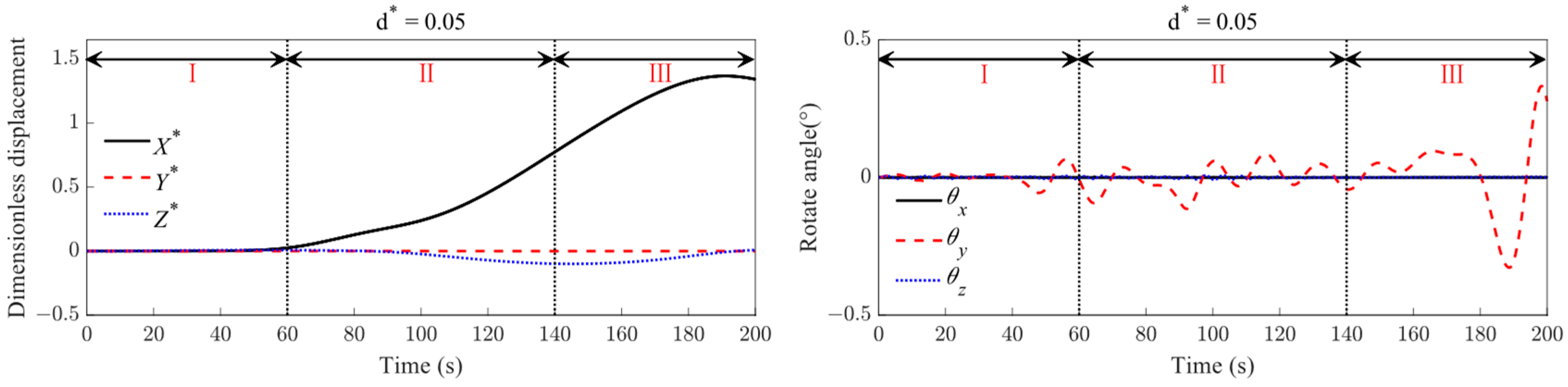
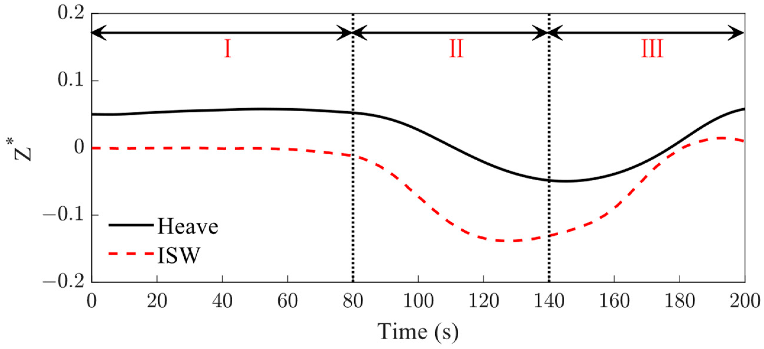
4.2. The Effect of the Initial Suspended Depth on the Motion Response of the Suspended Submersible

In Section 4.1, the interaction characteristics of a suspended submersible located at the upper layer of fluid ($d^{*}=0.05$) are discussed. The motion behaviors of the submersible at different initial submerged positions are significantly different, due to the flow field and density field. In order to explore the effects of the initial submerged depth on the dynamic kinematic properties of the suspended submersible, this section sets out eight cases with various initial suspended positions, as shown in

Table 2. Case setups of the submersible at eight different submerged positions under the ISW.

Position	$\mathbf{Distance} \mathbf{to} \mathbf{Pycnocline} ({\mathit{d}}^{\mathit{*}}$)	$\mathbf{Density} (\mathbf{k}\mathbf{g}/{\mathbf{m}}^3$)
Upper fluid	0.1	998
	0.05	998
Pycnocline	0	1013
Lower fluid	−0.05	1025
	−0.15	1025
	−0.25	1025
	−0.35	1025
	−0.45	1025

and Figure 16.

Figure 17 gives the velocity-vector contours to show the interaction process between the ISW fluid field and the suspended submersible at four different initial submerged depths ($d^{*}=0.05,0,-0.05, \mathrm{a}\mathrm{n}\mathrm{d}-0.15$). It can be found that the heave-motion characteristics of the submersible located at different positions are similar, while the significant differences exist in the longitudinal motion. Moreover, during the whole process, all the submersibles only move in the single medium and do not penetrate the wave surface. Considering the interaction effect between the ISW fluid field and the suspended submersible, in addition to focusing on the induced motions of the submersible under the ISW, the interference of the submersible’s motion on the ISW fluid field cannot be ignored. As shown in Figure 17, the ISW fluid field, especially for the wave surface, is significantly disturbed by the motions of the submersible; the interference effect of the submersible on the ISW fluid field becomes more significant as the submersible becomes close to the wave surface. However, the characteristic length of the submersible $L_{pp}$ is one order of magnitude smaller than the wavelength of the ISW ${\lambda }_{eKdV}$; the interference of the submersible’s motion on the ISW fluid field is relatively limited, and can usually be ignored in a practical physical context. However, in the laboratory experiment, the scale of the structure is frequently overestimated, which may result in some errors.

Figure 18 gives the motion responses of the suspended submersible at different submerged depths under the action of the ISW at the same wave amplitude (${\xi }_0^{*}=-0.15$). Due to the opposite flow velocity directions between the upper and lower layer of fluids, there are significant differences in the longitudinal motion response of the suspended submersible located at the upper and lower layer of fluid. When the suspended submersible is located at or above the wave interface ($d^{*}\ge 0$), the submersible driven by the ISW fluid field moves along the propagation direction of the ISW with significant longitudinal displacements. And the longitudinal motion amplitude of the submersible completely immersed in the upper layer of fluid ($d^{*}>0$) is much larger than that of the submersible located exactly at the fluid interface ($d^{*}=0$); the submersible located below the wave interface ($d^{*}<0$) undergoes significant directional changes twice in the longitudinal motion, and the submersible ultimately moves for a certain distance in the opposite direction of the ISW propagation, relative to its initial position. Its longitudinal motion amplitude is much smaller than that of the submersible located above the wave interface ($d^{*}>0$).

Moreover, for the submersible located in the same fluid medium ($d^{*}>0$ or $d^{*}<0$), the influence of the initial position of the submersible on the longitudinal motion response is not significant, while it leaves slight differences in the motion amplitude. Generally speaking, the longitudinal motion amplitude of the submersible slightly decreases with the increase in the distance from the submersible to the pycnocline in the vertical direction. And the longitudinal motion, characteristic of the submersible with the change in the submerged depth, is consistent with the vertical distribution which is a characteristic of the horizontal flow velocity in the internal-wave flow field; that is, the horizontal velocity of the flow field decreases with the increase in distance to the interface.

Regarding the heave motion, the motion characteristics of the submersible located at different initial suspended depths are similar. The submersible firstly dives to the dropping amplitude and then quickly floats up. However, the motion process of the suspended submersible located at the different positions in the heave direction still retain some differences, as shown in Figure 18b. When the suspended submersible dives to the dropping amplitude, the submersible at the wave interface ($d^{*}=0$) is located exactly at the trough, and the submersible at the upper fluid ($d^{*}>0$) is located above the trough, while the submersible at the lower fluid interface ($d^{*}<0$) is located just below the trough, as shown in Figure 17. The vertical motion of the submersible located at the fluid interface ($d^{*}=0$) is completely synchronized with the ISW surface. For the submersible located in the same medium ($d^{*}>0$ or $d^{*}<0$), the dropping amplitude of the submersible decreases and the time to reach the amplitude increases with an increase in the distance to the ISW interface. Moreover, the dropping amplitude of the submersible located at the lower layer of fluid ($d^{*}<0$) decreases almost proportionally with the increase in the vertical distance to the fluid interface, as shown in Figure 18e.

Regarding the pitch motion, there are significant differences in the longitudinal inclination angle of the submersibles located at different positions, as shown in Figure 18c,e. The pitch motion of the submersible ($d^{*}=0$) located at the interface always fluctuates with the ISW surface, and the pitch angle is always equal to the inclined angle of the wave at the submersible’s position, as shown in Figure 17b. When the submersible dives near the right-hand wave surface, its burial angle increases, due to the uneven distribution of the internal forces acting on the surface of the submersible. When the submersible dives to the ISW trough, its pitch angle returns to exactly zero degrees. When the submersible floats up on the left-hand wave surface, the bow angle of the submersible increases with the inclination angle of the wave. For the submersible located above the wave interface ($d^{*}>0$), there is little change in the pitch motion during the whole process. The submersible located below the wave interface ($d^{*}<0$) only generates a small inclination angle while approaching the core fluid field, and the amplitude of the inclination angle is less than 3°. Similarly, the amplitude of the longitudinal inclination angle decreases as its relative distance to the wave surface increases.

Figure 18d shows the overall motion trajectory of the submersible under the action of the internal wave field. The motion trajectory of the submersible located at the lower layer of fluid ($d^{*}<0$) is exactly the same as the trace of the fluid field, and its shape is like an unclosed clockwise ellipse. As the submerged depth increases, the longitudinal motion responses of the submersible are not affected, but its vertical motion response decreases proportionally, and its motion trajectory becomes flatter. The motion trajectory of the submersible located at the interface ($d^{*}=0$) is shaped like a “V” shape; the trajectory of the submersible located at the upper fluid ($d^{*}>0$) is shaped like a counterclockwise semi ellipse, with large eccentricity.

4.3. The Effect of the Wave Amplitude on the Motion Response of the Suspended Submersible

The ISW fluid field with the largest wave amplitude has higher induced flow velocity, which may result in a huge potential threat to underwater vehicles. In order to investigate the effect of the wave amplitude on the motion responses of the suspended submersible, in this section, six simulation cases for the submersible located at the upper- and lower-fluid layer ($d^{*}=0.05$, $d^{*}=-0.05$) under the ISW at three different ISW amplitudes (${\xi }_0^{*}=-0.1,-0.15, \mathrm{a}\mathrm{n}\mathrm{d}-0.2$) are set, and the other parameters are the same as in Section 4.1, as shown in

Table 3. Case setups of the two submersibles located at the upper- and lower-fluid layer under the ISW with three different amplitudes.

Position	$\mathbf{Distance} \mathbf{to} \mathbf{Pycnocline} ({\mathit{d}}^{\mathit{*}}$)	$\mathbf{ISW} \mathbf{Amplitude} ({\mathit{\xi }}_0^{\mathit{*}}$)
Upper layer of fluid	0.05	$-$0.1
		$-$0.15
		$-$0.2
Lower layer of fluid	$-$0.05	$-$0.1
		$-$0.15
		$-$0.2

and Figure 19.

Figure 20 gives the motion responses of the suspended submersible located at the upper layer of fluid ($d^{*}=0.05$) and the lower layer of fluid ($d^{*}=-0.05$) under the action of the ISW at three different ISW amplitudes (${\xi }_0^{*}=-0.1,-0.15,-0.2$). The driven motion characteristics of the suspended submersible under the ISW at different wave amplitudes are similar, and only leave some differences in its motion amplitudes. With an increase in the amplitude of the ISW, the motion amplitude of the submersible increases, especially in the surge and heave directions. However, the influence of the ISW amplitude acting on the pitch motion of the submersible is not significant compared with the above-mentioned two directions. And the submersible reaches its motion amplitude in the pitch direction while approaching the core fluid field of the ISW.

For the submersible located at the lower layer of fluid ($d^{*}=-0.05$), due to the complexity of the flow field at the lower layer of fluid, the surge motion of the submersible has significant directional changes. Moreover, the time for the submersible to reach the motion amplitude in the surge and heave directions decreases as the wave amplitude increases. However, for the submersible at the upper layer of fluid ($d^{*}=0.05$), with an increase in the wave amplitude, the surge motion is almost completely synchronized and the motion amplitude also increases proportionally.

As shown in Figure 20, the motion trajectory of the submersible located at the upper layer of fluid ($d^{*}=0.05$) is a clockwise semi ellipse, while the trajectory of the submersible located at the lower fluid ($d^{*}=-0.05$) is shaped like an unclosed counterclockwise ellipse. The amplitude of the ISW does not change the shape of the motion trajectory, but only determines the amplitude of its motion trajectory. The range of the motion trajectory of the submersible in the x-o-z plane significantly increases with an increase in the ISW amplitude.

5. Conclusions

In this paper, a three-dimensional interaction numerical model between the suspended submersible and the ISW fluid field is established, based on the CFD method. Based on the conducted numerical model, we investigated the dynamic interaction characteristics of the suspended submersible under the action of the ISW field. The effects of the initial suspended depths and the ISW amplitudes on the motion responses of the submersible are also discussed. The conclusions of this paper are drawn as follows:

(1)

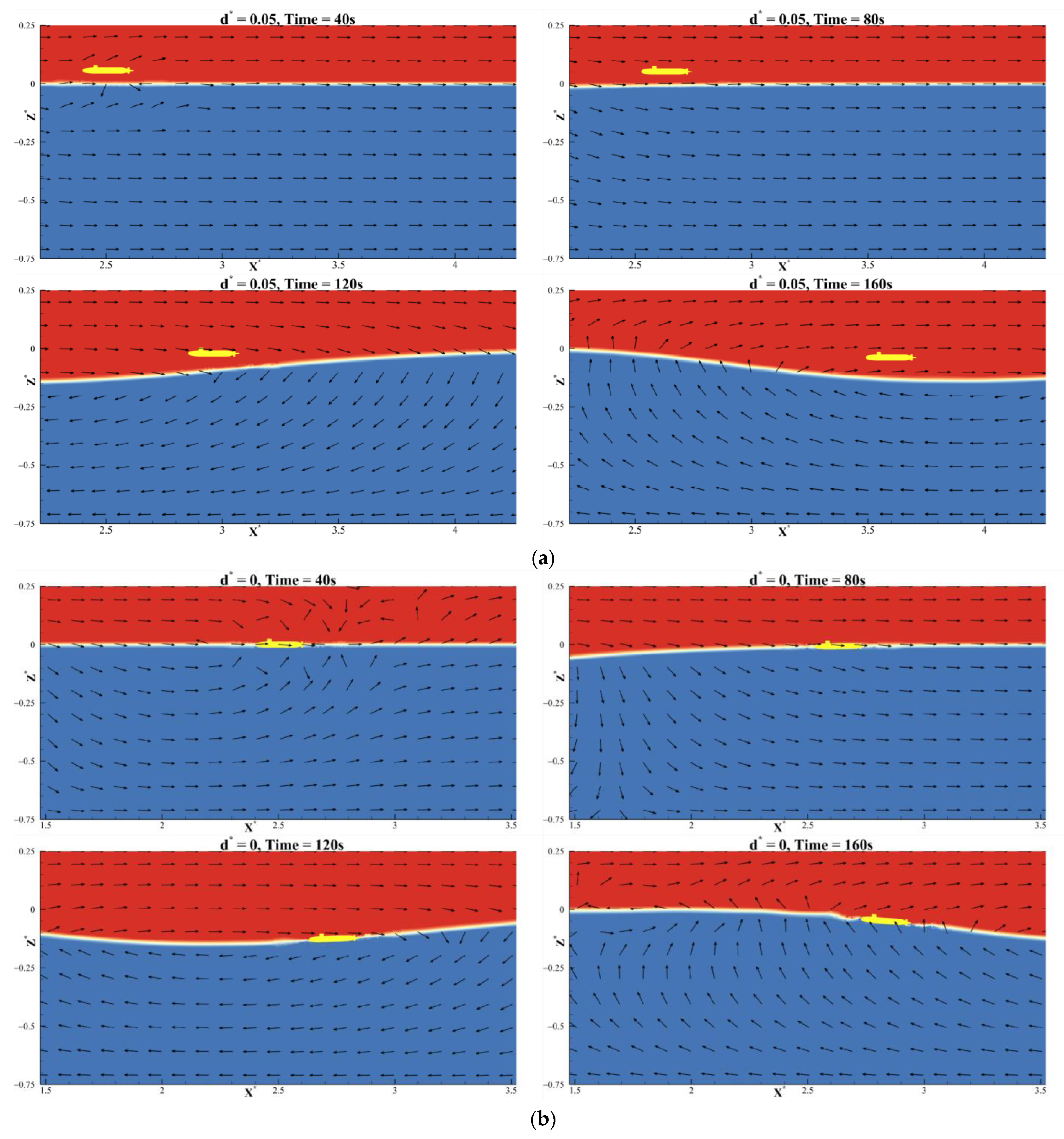
When the suspended submersible encounters the ISW fluid field, the motions of the submersible in the x-o-z plane change significantly. The submersible always drifts with the nearby ISW surface, gradually dives to the dropping amplitude, and then floats quickly under the action of the ISW fluid field. During the whole motion process, the submersible does not penetrate the wave surface. Moreover, the change in the pitch angle is not significant, due to the action of its own stability.

(2)

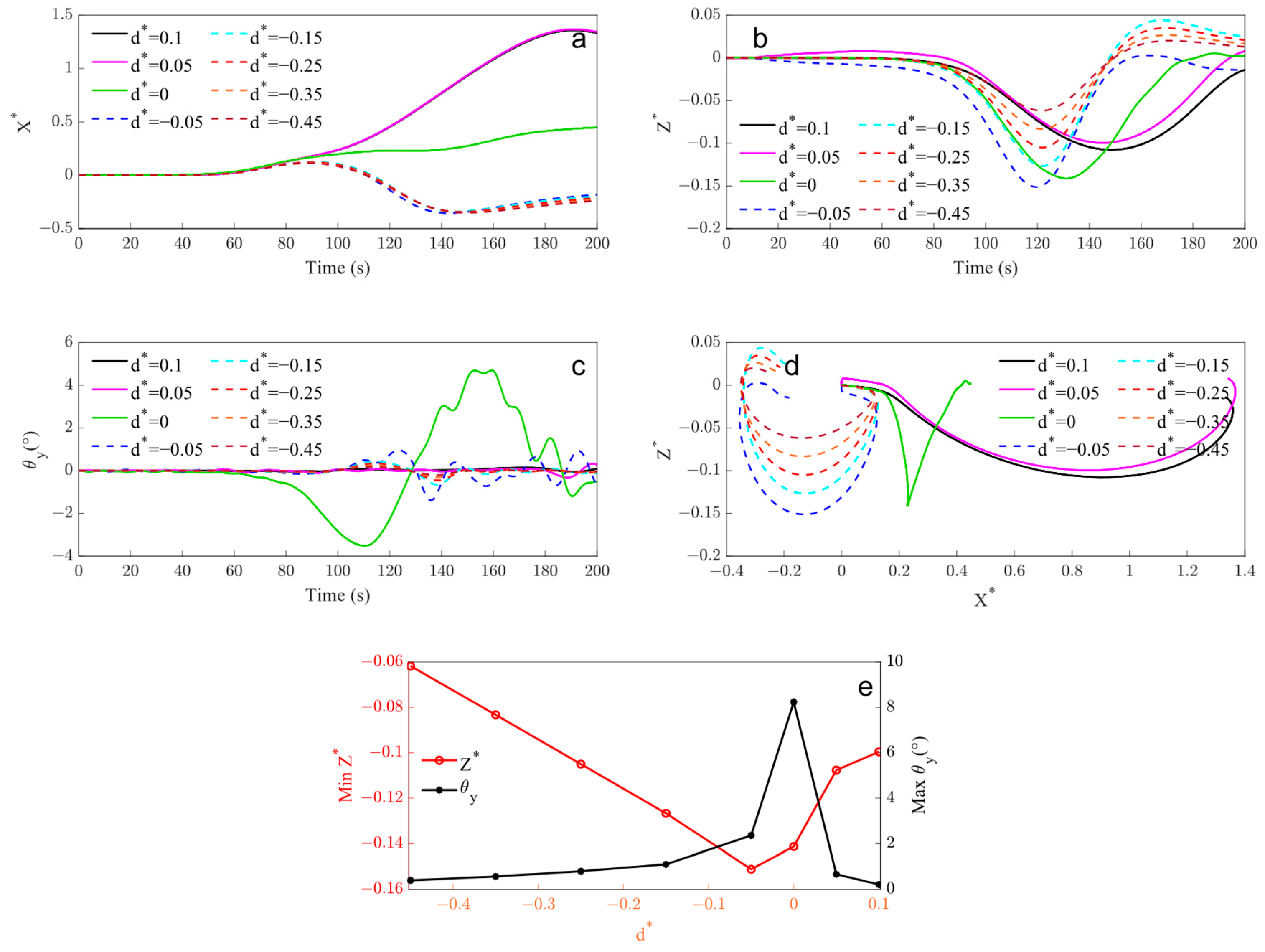
The initial submerged depth of the submersible is a key factor determining the motion response mode: the submersibles located at the wave interface and upper fluid layer ($d^{*}\ge 0$) continue to move for a large distance along the propagation direction of the ISW. The motion trajectory of the submersible immersed in the upper layer ($d^{*}>0$) is similar to an unclosed clockwise ellipse, while that of the submersible at the wave interface ($d^{*}=0$) is similar to a “V” shape. The submersible at the lower layer of fluid ($d^{*}<0$) undergoes directional change movements twice in the longitudinal direction and its motion trajectory presents as an unclosed ellipse, in a clockwise direction.

(3)

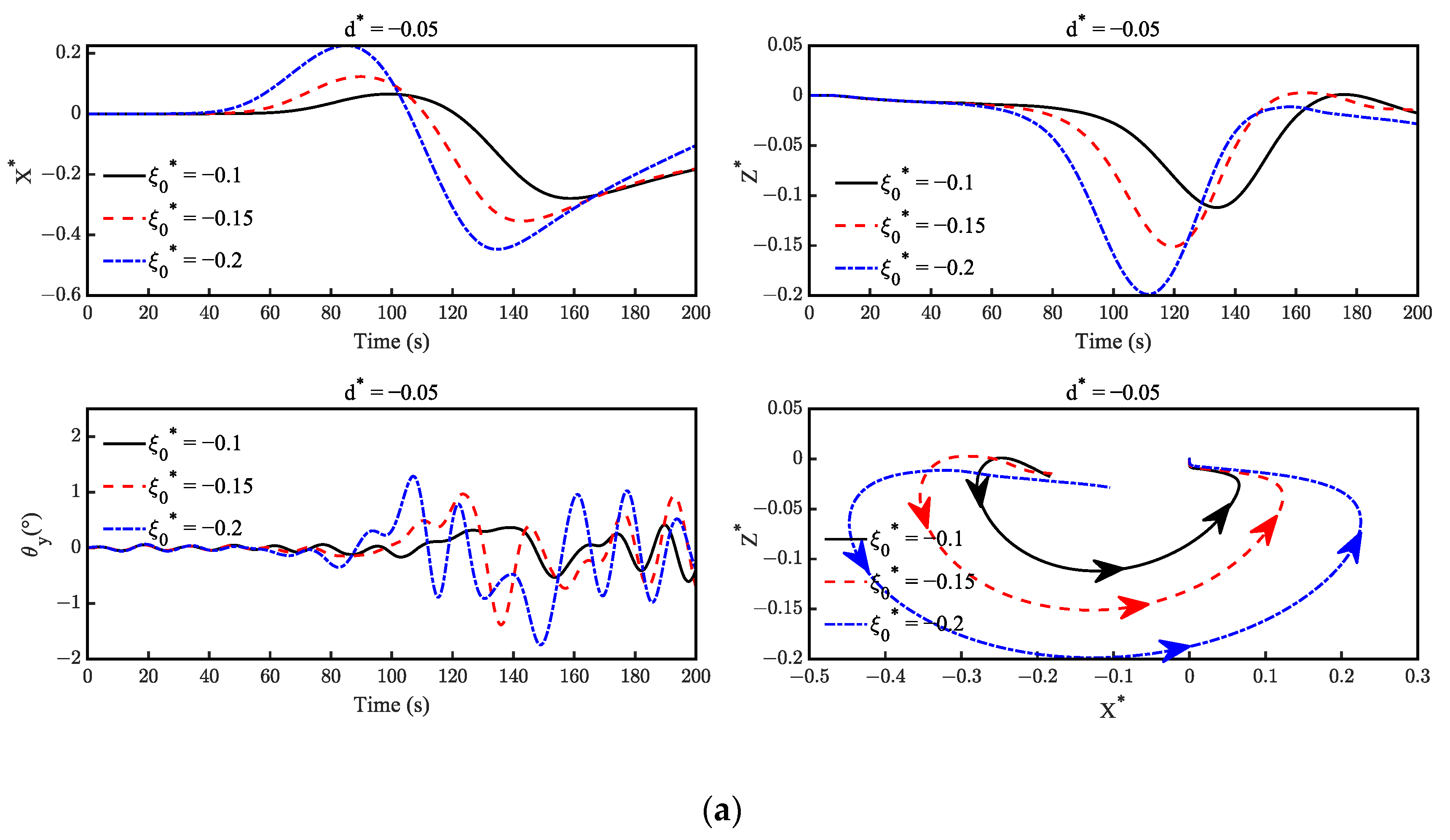
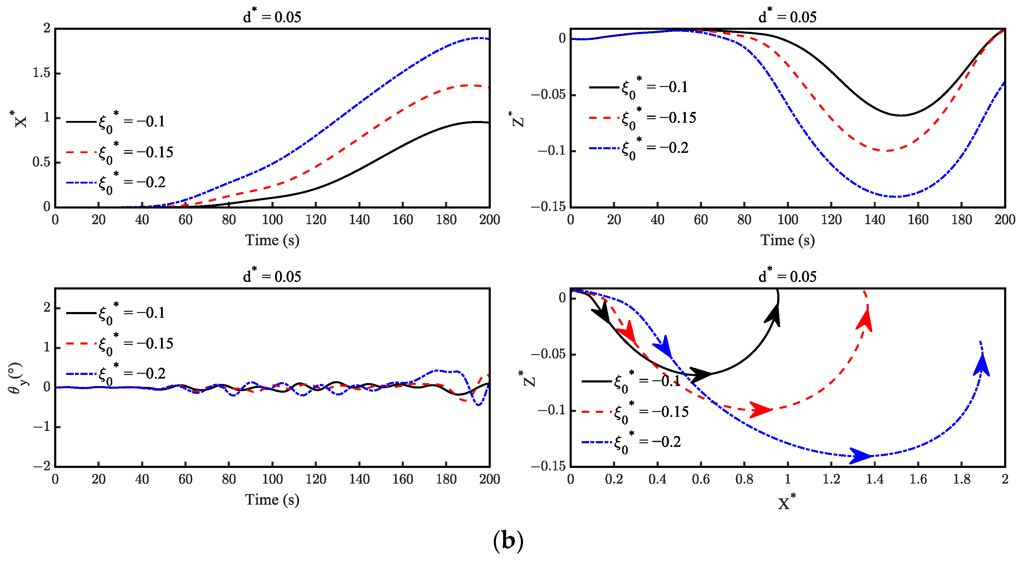
For the submersible located in the same medium ($d^{*}>0$ or $d^{*}<0$), the longitudinal motion is almost unaffected by its initial suspended depth. However, the amplitude of the surge motion slightly increases as the distance to the interface decreases, which is completely consistent with the vertical distribution characteristics of the horizontal velocity in the ISW flow field. The amplitude of the heave motion decreases as the vertical distance from the submersible to the wave interface increases.

(4)

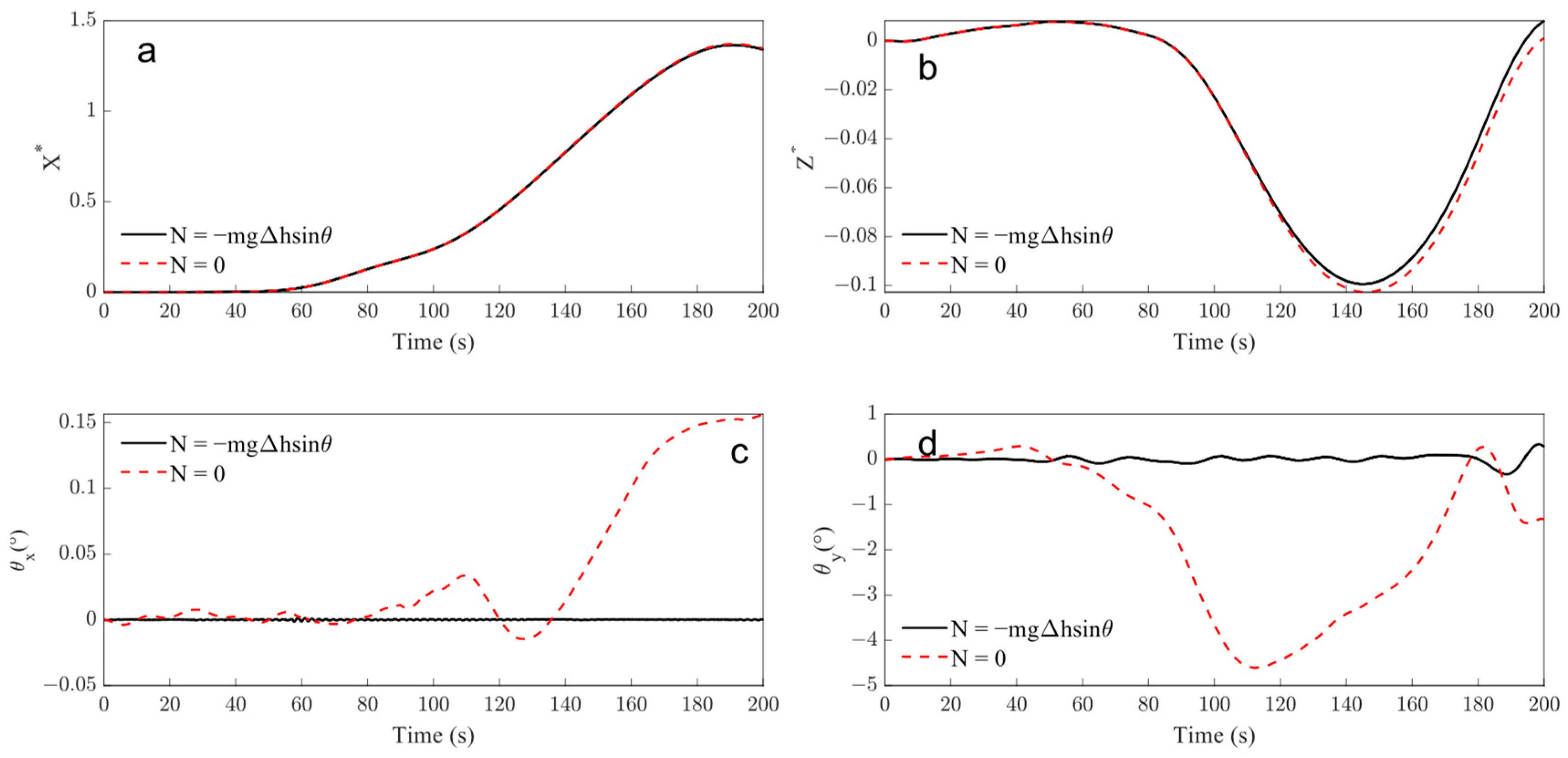
In the case of the submersible located at the pycnocline ($d^{*}=0$), it would always adhere to the ISW surface; its pitch angle changes significantly with the fluctuation of the ISW surface, which may be the most dangerous condition for the submersible.

(5)

The amplitude of the ISW only influences the planar motion amplitude of the submersible and does not determine its natural motion characteristic. The motion responses of the submersible increase with the increase in the amplitude of the ISW. Especially for the heave direction, the amplitude of the submersible even increases proportionally with the increase in the amplitude of the ISW. Moreover, the influence of the amplitude of the ISW, acting on the pitch motion of the submersible, is not significant.

It is worth noting that this paper only investigates the interaction mechanism between the suspended submersible and the ISW. In the future, we could investigate the dynamic responses of the submersible with the propulsive capability of the ISW. Moreover, it is also valuable to explore the interaction effect between the submersible and other types of waves, to enhance the safety and maneuverability of the submersible.

References

- Garrett, C.; Munk, W. Internal waves in the ocean. Annu. Rev. Fluid Mech. 1979, 11, 339–369. [Google Scholar] [CrossRef]
- Osborne, A.R.; Burch, T.L. Internal solitons in the Andaman Sea. Science 1980, 208, 451–460. [Google Scholar] [CrossRef] [PubMed]
- Ebbesmeyer, C.C.; Coomes, C.A.; Hamilton, R.C.; Kurrus, K.A.; Sullivan, T.C.; Salem, B.L.; Romea, R.D.; Bauer, R.J. New observations on internal waves (solitons) in the South China Sea using an acoustic Doppler current profiler. Mar. Technol. Soc. J. 1991, 91, 165–175. [Google Scholar]
- Vlasenko, V.; Stashchuk, N.; Guo, C.; Chen, X. Multimodal structure of baroclinic tides in the South China Sea. Nonlinear Process. Geophys. 2010, 17, 529–543. [Google Scholar] [CrossRef]
- Huang, X.; Chen, Z.; Zhao, W.; Zhang, Z.; Zhou, C.; Yang, Q.; Tian, J. An extreme internal solitary wave event observed in the northern South China Sea. Sci. Rep. 2016, 6, 30041. [Google Scholar] [CrossRef]
- Zhang, M.; Hu, H.; Du, P.; Chen, X.-P.; Li, Z.; Wang, C.; Cheng, L.; Tang, Z. Detection of an internal solitary wave by the underwater vehicle based on machine learning. Phys. Fluids 2022, 34, 115137. [Google Scholar] [CrossRef]
- Gong, Y.; Xie, J.; Xu, J.; Chen, Z.; He, Y.; Cai, S. Oceanic ISWs at the Indonesian submersible wreckage site. Acta Oceanol. Sin. 2022, 41, 109–113. [Google Scholar] [CrossRef]
- Wang, T.; Huang, X.D.; Zhao, W.; Zheng, S.H.; Yang, Y.C.; Tian, J.W. Internal Solitary Wave Activities near the Indonesian Submarine Wreck Site Inferred from Satellite Images. J. Mar. Sci. Eng. 2022, 10, 197. [Google Scholar] [CrossRef]
- Chen, M.; Chen, K.; You, Y. Experimental investigation of internal solitary wave forces on a semi-submersible. Ocean Eng. 2017, 141, 205–214. [Google Scholar] [CrossRef]
- Chen, M.; Chen, J.; You, Y.X. Forces on a semi-submersible in internal solitary waves with different propagation directions. Ocean Eng. 2020, 217, 107864. [Google Scholar] [CrossRef]
- Cui, J.; Dong, S.; Wang, Z.; Han, X.; Yu, M. Experimental research on internal solitary waves interacting with moored floating structures. Mar. Struct. 2019, 67, 102641. [Google Scholar] [CrossRef]
- Russo, S.; Contestabile, P.; Bardazzi, A.; Leone, E.; Iglesias, G.; Tomasicchio, G.R.; Vicinanza, D. Dynamic loads and response of a spar buoy wind turbine with pitch-controlled rotating blades: An experimental study. Energies 2021, 14, 3598. [Google Scholar] [CrossRef]
- Wang, S.D.; Wei, G.; Du, H.; Wu, J.L.; Wang, X.L. Experimental investigation of the wave-flow structure of an oblique internal solitary wave and its force exerted on a slender body. Ocean Eng. 2020, 201, 107057. [Google Scholar] [CrossRef]
- Wang, S.; Du, H.; Wei, G.; Peng, P.; Xuan, P.; Xu, J. Effects of the inhomogeneous vertical structure of an internal solitary wave on the force exerted on a horizontal transverse cylinder. Phys. Fluids 2023, 35, 062117. [Google Scholar] [CrossRef]
- Cui, J.; Dong, S.; Wang, Z.; Han, X.; Lv, P. Kinematic response of submerged structures under the action of internal solitary waves. Ocean Eng. 2020, 196, 106814. [Google Scholar] [CrossRef]
- Cui, J.; Dong, S.; Wang, Z.; Cheng, J.; Ren, J. Experimental study on motion response of a submersible spherical model under the action of internal solitary wave propagating over a ridge topography. Ocean Eng. 2022, 258, 111700. [Google Scholar] [CrossRef]
- Cai, S.; Long, X.; Gan, Z. A method to estimate the forces exerted by internal solitons on cylindrical piles. Ocean Eng. 2003, 30, 673–689. [Google Scholar] [CrossRef]
- Cai, S.; Wang, S.; Long, X. A simple estimation of the force exerted by internal solitons on cylindrical piles. Ocean Eng. 2006, 33, 974–980. [Google Scholar] [CrossRef]
- Cai, S.; Long, X.; Wang, S. Forces and torques exerted by internal solitons in shear flows on cylindrical piles. Appl. Ocean Res. 2008, 30, 72–77. [Google Scholar] [CrossRef]
- Feng, K.; Yao, Z.; Hu, F.; Liu, L. Motion simulation of submersible passing through internal solitary wave. Chin. J. Hydrodyn. 2022, 37, 467–473. [Google Scholar]
- Liu, X.; Gou, Y.; Teng, B. Research on the Trajectory and Gesture of a Slender Submarine Undergoing Significant Motion Under the Action of Internal Solitary Waves. Chin. J. Acta Armamentarii 2023, 1–12. [Google Scholar]
- Liu, M.; Wei, G.; Sun, Z. Motion response of a horizontal slender submerged ellipsoid induced by head-on interfacial solitary waves. In Proceedings of the 30th National Hydrodynamics Symposium and the 15th National Hydrodynamics Academic Conference, Hefei, China, 16–19 August 2019; pp. 247–254. [Google Scholar]
- Junrong, W.; Junfeng, D.; Min, Z.; Anteng, C. An Iterative Updating Method for Dynamic Responses of a Floating Platform Under Action of Internal Solitary Waves. In Proceedings of the ASME 38th International Conference on Ocean, Offshore and Arctic Engineering, Glasgow, UK, 9–14 June 2019; American Society of Mechanical Engineers: New York, NY, USA, 2019; Volume 58769. [Google Scholar]
- Cheng, S.; Yu, Y.; Li, Z.; Huang, Z.; Yang, Z.; Zhang, X.; Cui, Y.; Wu, J.; Liu, X.; Yu, J. The influence of internal solitary wave on semi-submersible platform system including mooring line failure. Ocean Eng. 2022, 258, 111604. [Google Scholar] [CrossRef]
- Li, J.; Zhang, Q.; Chen, T. Numerical Investigation of internal solitary wave forces on submersibles in continuously stratified fluids. J. Mar. Sci. Eng. 2021, 9, 1374. [Google Scholar] [CrossRef]
- He, G.; Xie, H.; Zhang, Z.; Liu, S. Numerical Investigation of internal solitary wave forces on a moving submersible. J. Mar. Sci. Eng. 2022, 10, 1020. [Google Scholar] [CrossRef]
- Ding, W.; Sun, H.; Zhao, X.; Ai, C. Numerical study of the interaction between an internal solitary wave and a submerged extended cylinder using OpenFOAM. Ocean Eng. 2023, 274, 113985. [Google Scholar] [CrossRef]
- Cheng, L.; Du, P.; Hu, H.; Xie, Z.; Yuan, Z.; Kaidi, S.; Chen, X.; Xie, L.; Huang, X.; Wen, J. Control of underwater suspended vehicle to avoid ‘falling deep’ under the influence of internal solitary waves. Ships Offshore Struct. 2023, 1–19. [Google Scholar] [CrossRef]
- Wang, J.; He, Z.; Xie, B.; Zhuang, C.; Wu, W. Numerical investigation on the interaction between internal solitary wave and self-propelled submersible. Phys. Fluids 2023, 35, 107119. [Google Scholar] [CrossRef]
- Wang, C.; Wang, J.; Liu, Q.; Zhao, S.; Li, Z.; Kaidi, S.; Hu, H.; Chen, X.; Du, P. Dynamics and “falling deep” mechanism of submerged floating body under internal solitary waves. Ocean Eng. 2023, 288, 116058. [Google Scholar] [CrossRef]
- Chen, H.C.; Patel, V.C.; Ju, S. Solutions of Reynolds-averaged Navier-Stokes equations for three-dimensional incompressible flows. J. Sci. Comput. Phys. 1990, 88, 305–336. [Google Scholar] [CrossRef]
- Yakhot, V.; Orszag, S. Renormalization group analysis of turbulence. I. Basic theory. J. Sci. Comput. 1986, 1, 3–51. [Google Scholar] [CrossRef]
- Wang, J.; Shi, C.; Wang, H.D.; He, C. Dynamic analysis and swing suppression method of a “Mooring-HLC-Cargo” coupled system. Ocean Eng. 2024, 295, 116840. [Google Scholar] [CrossRef]
- Gertler, M.; Hagen, G.R. Standard Equations of Motion for Submersible Simulation; NSRDC Report 2510; Defense Technical Information Center: Fort Belvoir, VA, USA, 2020. [Google Scholar]
- He, G.; Zhang, C.; Xie, H.; Liu, S. The Numerical Simulation of a Submarine Based on a Dynamic Mesh Method. J. Mar. Sci. Eng. 2022, 10, 1417. [Google Scholar] [CrossRef]
- Yu, T.; Chen, X.; Tang, Y.; Wang, J.; Wang, Y.; Huang, S. Numerical modelling of wave run-up heights and loads on multi-degree-of-freedom buoy wave energy converters. Appl. Energy 2023, 344, 121255. [Google Scholar] [CrossRef]
- Koop, C.; Butler, G. An investigation of ISWs in a two-fluid system. J. Fluid Mech. 1981, 112, 225–251. [Google Scholar] [CrossRef]
- Michallet, H.; Barthelemy, E. Experimental study of interfacial solitary waves. J. Fluid Mech. 1998, 366, 159–177. [Google Scholar] [CrossRef]
- Choi, W.; Camassa, R. Fully nonlinear internal waves in a two-fluid system. J. Fluid Mech. 1999, 396, 1–36. [Google Scholar] [CrossRef]
- Miyata, M. An internal solitary wave of large amplitude. La Mer 1985, 23, 43–48. [Google Scholar]
- Turkington, B.; Eydeland, A.; Wang, S. A computational method for solitary internal waves in a continuously stratified fluid. Stud. Appl. Math. 1991, 85, 93–127. [Google Scholar] [CrossRef]
- Craig, W.; Guyenne, P.; Kalisch, H. Hamiltonian long-wave expansions for free surfaces and interfaces. Commun. Pure Appl. Math. 2005, 58, 1587–1641. [Google Scholar] [CrossRef]
- Kakutani, T.; Yamasaki, N. Solitary waves on a two-layer fluid. J. Phys. Soc. Jpn. 1978, 45, 674–679. [Google Scholar] [CrossRef]
- Kang, X.L.; Wang, J.R.; Xie, B.T.; He, Z.Y. Numerical Study on the Fluid Structure Interaction of internal Solitary Waves and a Spar-Type FOWT. J. Ocean Univ. China 2023, 53, 98–105. [Google Scholar]
- Groves, N.; Huang, T.; Chang, M. Geometric Characteristics of DARPA (Defense Advanced Research Projects Agency) SUBOFF Models (DTRC Model Numbers 5470 and 5471); David Taylor Research Center Bethesda MD Ship Hydromechanics Department; Defense Technical Information Center: Fort Belvoir, VA, USA, 1989. [Google Scholar]
- Liu, H.; Huang, T. Summary of DARPA SUBOFF Experimental Program Data; Naval Surface Warfare Center Carderock Div Bethesda MD Hydromechanics Directorate; Defense Technical Information Center: Fort Belvoir, VA, USA, 1998. [Google Scholar]
- Liu, S.; He, G.H.; Zhang, Z.G.; Hu, C.H.; Zhang, C.; Wang, Z.K.; Xie, H.F. Multi-Parameter Influence Analysis of Interaction Between Internal Solitary Wave and Fixed Submerged Body. Chin. Ocean Eng. 2023, 37, 934–947. [Google Scholar] [CrossRef]
- Duan, J.; Wang, X.; Zhou, J.; You, Y. Effect of internal solitary wave on the dynamic response of a flexible riser. Phys. Fluids 2023, 35, 017107. [Google Scholar] [CrossRef]
- Sukas, O.F.; Kinaci, O.K.; Cakici, F.; Gokce, M.K. Hydrodynamic assessment of planing hulls using overset grids. Appl Ocean Res. 2017, 65, 35–46. [Google Scholar] [CrossRef]