Application of a Statistical Regression Technique for Dynamic Analysis of Submarine Pipelines

Abstract

This study employs a statistical regression technique to investigate the maximum displacement, stress, and natural vibration frequencies of a submarine pipeline subjected to hydrodynamic wave forces. Eighteen pipeline models are designed, varying in wall thickness from 10 mm to 30 mm and diameter from 500 mm to 1000 mm. The hydrodynamic drag and inertia forces are performed by using the Morison equation. Computer-aided Finite Element Analysis is employed to simulate the complex interactions between the fluid and structure in 18 pipelines. Multiple Regression technique is used to evaluate the reliability metrics, considering uncertainties in geometrical properties affecting pipeline performance. Full Quadratic models are developed for expressing more effective and concise mathematical equations. Analysis of Variance (ANOVA) is performed to determine the adequacy of the model in representing the observed data. The Coefficient of Determination (R²), Mean Square Error (MSE), and Mean Absolute Error (MAE) are calculated to assess the equation’s predictive accuracy and reliability. The results confirm the suitability of the suggested regression technique for analyzing the relationships between predictor variables and the response variable.

1. Introduction

The design of submarine pipelines involves a comprehensive approach that integrates knowledge from multiple disciplines, aiming to ensure the long-term integrity and functionality of critical components in the oil and gas industry’s transportation infrastructure. Environmental loads, including wave forces, are carefully analyzed, with particular attention to the physical properties of the water and the characteristics of the pipeline itself, such as diameter (D), thickness (t), and material composition. Additionally, factors like wave height (H), wave period (T), and water depth (d) play a significant role in influencing hydrodynamic processes and the dynamic behaviors of pipelines. Researchers have proposed different methodologies, such as numerical modeling, experimental testing, field measurements, and fault detection techniques in subsea environments, to analyze and mitigate stability concerns [1,2,3,4,5,6,7]. Repeated and complex analyses are performed under variable conditions to determine the structural design.

In recent years, where the importance of achieving results in a shorter time and with fewer resources has increased, the use of statistical prediction methods in the analysis of submarine pipelines has also increased. Youssef et al. employ a statistical method to create a response surface model that predicts the maximum horizontal displacement of a pipeline during storm conditions. The Monte Carlo simulation technique is applied alongside the established response surface model to determine extreme response statistics [8]. Xu and Sinha introduce a thorough analytical structure for statistically analyzing field performance data for water pipelines. The paper provides a detailed explanation of the methodology’s implementation steps, along with preliminary analyses conducted on datasets from two different water utility systems [9]. The study by Zhang and Weng presents a Bayesian network model for analyzing buried gas pipeline failures caused by corrosion and external interference. The model offers a probabilistic framework for assessing the risk of pipeline failure, taking into account various contributing factors and their uncertainties [10]. Zhang et al. develop an optimal statistical regression model capable of predicting the wave-induced equilibrium scour depth beneath pipelines in sandy and silty seabeds [11]. Most of the studies conducted on offshore structures are based on ground movements occurring on the seabed [12,13]. In this study, a suspended pipeline model is examined to avoid the impact of seabed movement.

This study aims to provide a more comprehensive understanding of the factors influencing pipeline dynamic behavior and to enhance the accuracy of stability assessments by using statistical methods. This study focuses on the structural model rather than seabed movement and material properties. This approach allows for a comprehensive assessment of pipeline stability under hydrodynamic wave forces, enabling informed decision-making in design processes.

The multiple regression model, which is most commonly used for complex decision problems in many fields [14], is employed to demonstrate the general tendencies of the relationship between the pipeline design parameters and stability criteria. The hydrodynamic wave forces are obtained by using Airy Wave Theory. Le Méhauté’s diagram is used to determine the applicability theories of water waves according to the values of normalized wave height H and the water depth d [15]. The hydrodynamic drag force (F_D) and inertia force (F_M) are performed by using the Morison equation. Since the ratio of the gap between the pipe and the seabed to the pipe diameter is considered to be greater than 1.0, the hydrodynamic lift force (F_L) has been neglected [16]. The vibration and stability of a simply supported steel pipeline are analyzed when lateral hydrodynamic forces (F_H) act on it. For this, the dynamic behavior of the pipeline is modeled by computer-aided Time History Analyses based on Newmark β [17]. The pipe wall thickness ranges from 10 to 30 mm, and the pipe outer diameter ranges from 500 to 1000 mm. The initial three natural frequencies, maximum values of stress, and displacement are used to create a dataset to explore relationships between variables for 18 pipe models. The multiple regression method is employed to assess the reliability metrics while accounting for uncertainties in the geometric properties that influence pipeline performance. Full quadratic models are constructed to present more efficient and concise mathematical formulations. An Analysis of Variance is conducted to ascertain the model’s adequacy in accurately representing the collected data. The performance of the regression methods is evaluated based on different metrics: Mean Squared Error (MSE), Mean Absolute Error (MAE), and Coefficient of Determination (R²). The results highlighted that the proposed regression methods can be an alternative practical way that provides the correct solution in a shorter time in the preliminary design of submarine pipelines. The relationship between the variables can be implemented in any computational calculation software.

2. Analyzing Procedure

In this paper, a 2D structural model is performed to predict the dynamic behavior of submarine pipelines under wave forces according to displacements, maximum stresses, and natural vibration frequencies. Airy Wave Theory is used to obtain wave forces, which are adopted as environmental loads. Numerical simulations are also applied using the Time History Tool of SAP 2000. The natural vibration frequencies, maximum values of stress, and deflection are derived to create a dataset for the regression process. The multiple regression model is used to learn relationships between four categories of input and five categories of output from example data and to predict novel inputs. Moreover, 144 input values are used for estimating the relationships between dependent and independent variables for each case. The performance metrics of full quadratic equations have demonstrated that regression analyses can be used for forecasting and predicting submarine pipeline reactions based on geometrical properties and effective hydrodynamic forces.

2.1. Structural Model Application

In application, the predominant configuration of suspended submarine pipelines consists of multiple spans (refer to Figure 1), with support provided at intermediate locations through various support mechanisms. In this study, the pipe is selected as similar to the one used in Gücüyen [18], having L_p = 10 m span length and consisting of uniform and homogeneous material.

The structural behavior of the 18 pipe models is achieved under regular waves. The outside diameters of the pipe range from ϕ500 to ϕ1000, and the wall thicknesses are chosen as 10 mm, 20 mm, and 30 mm to verify the effect of cross-section on frequency, stress, and displacement values. The properties of the pipe models are given in

Table 1. Properties of the pipe models.

Model	P1	P2	P3	P4	P5	P6	P7	P8	P9
D (mm)	500	500	500	600	600	600	700	700	700
tw (mm)	10	20	30	10	20	30	10	20	30
Model	P10	P11	P12	P13	P14	P15	P16	P17	P18
D (mm)	800	800	800	900	900	900	1000	1000	1000
tw (mm)	10	20	30	10	20	30	10	20	30

.

The material properties of the pinned–pinned pipe are chosen to represent the steel, with Young’s modulus of 21 × 10⁷ kN/m², Poisson’s ratio of 0.3, and density of 78.50 kN/m³. Various combinations of pipe geometrical properties are performed using Time History analyses. The outer diameter of pipe models influences the value of hydrodynamic forces [19,20]. However, the wall thickness changes the behavior of the pipe in response to the force.

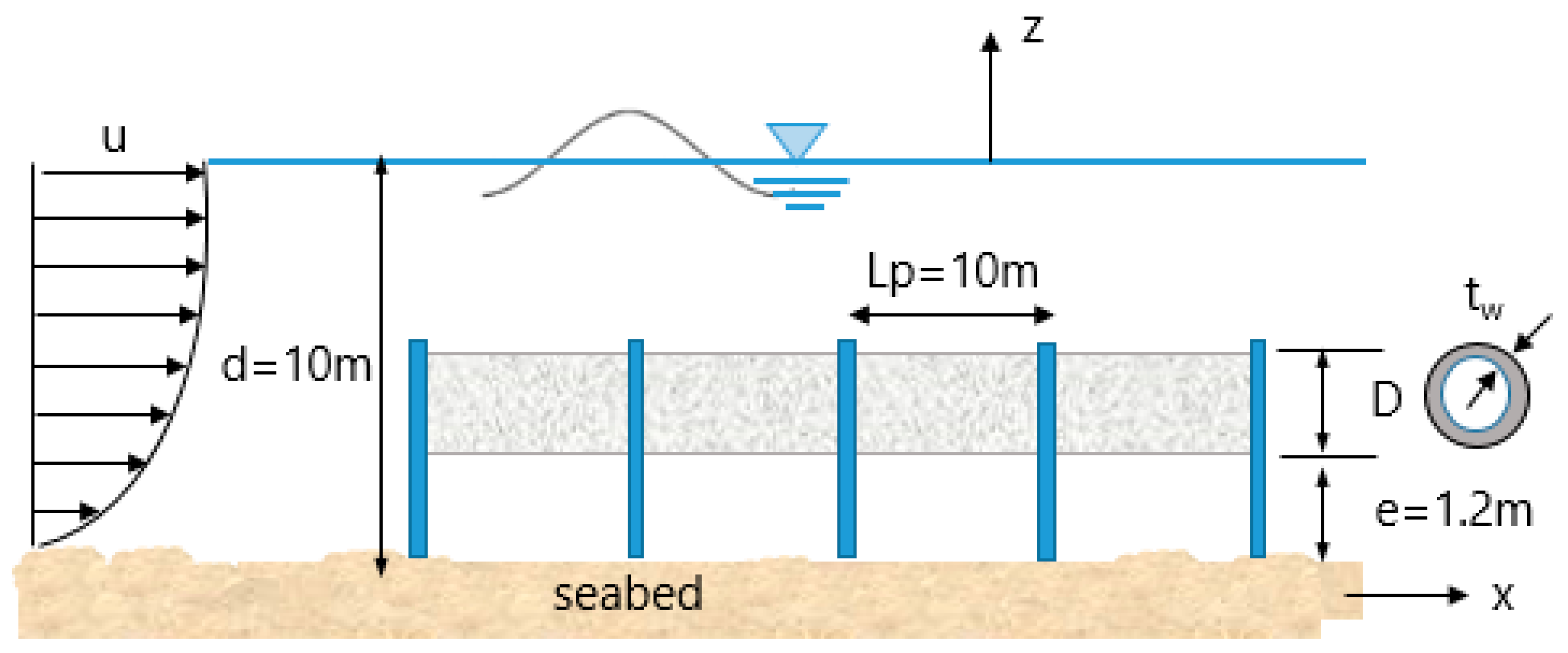
2.2. Environmental Conditions and Load Assessment

The submarine pipeline is designed by considering a combination of dead loads and wave loads. The environmental conditions are modeled in the numerical analysis based on Airy Wave Theory, referring to Le Méhauté’s diagram, which indicates the validity domain of each theory-type of water waves [21].

Water depth, wave period, and height are three major parameters in the design of marine facilities [22]. The employed parameters d = 10.00 m, T = 8.00 s, and H = 0.31 m are considered for the applicability criteria of Airy Wave Theory, which is widely used to model a marine environment [23]. The wave loads are calculated with water particle velocities (u) and accelerations ($\dot{u}$) by two different approaches presented as follows:

$$u=\frac{HgT}{2L}\frac{\cosh \left[2\pi \left(z+d\right)/L\right]}{\cosh \left(2\pi d/L\right)}\cos \left(\frac{2\pi }{L}x-\frac{2\pi }{T}t\right)$$

(1)

$$\dot{u}=\frac{g\pi H}{L}\frac{\cosh \left[2\pi \left(z+d\right)/L\right]}{\cosh \left(2\pi d/L\right)}\sin \left(\frac{2\pi }{L}x-\frac{2\pi }{T}t\right)$$

(2)

where the z-axis is directed vertically upward from the still water level, which is positive. The x-axis is along the direction of the propagation of waves. When the value of the relative water depth (water depth/wavelength, d/L) is between 0.005 and 0.05, it is classified as an intermediate depth wave, as mentioned in this study [24]. The free surface elevation η during the wave generation process is obtained based on the potential flow approach and is given in Figure 2.

The seawater characteristics are assigned as fluid properties, with a salty water density (ρ) of 1025 kg/m³ and a dynamic viscosity (μ) of 0.0015 Ns/m². The wavelength (L) is determined as ≈70.90 m by considering wave parameters.

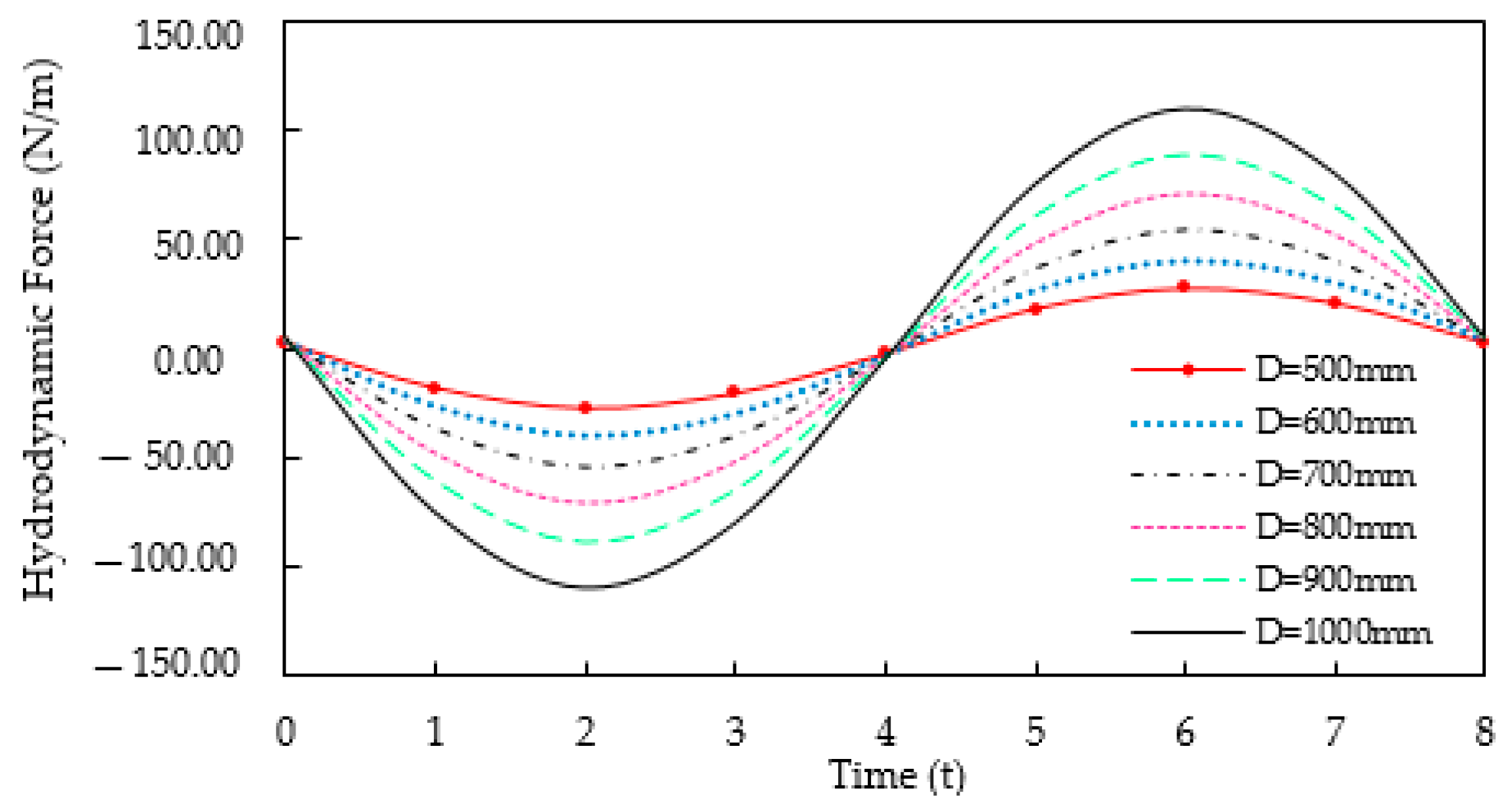
Description of Hydrodynamic Loads Acting on Pipeline

Drag, lift, and inertia forces are hydrodynamic loads caused by the motion of the surrounding water in a pipe. Drag and inertia are defined as the components that are parallel to the flow direction, and lift is the component of the hydrodynamic load that is perpendicular to the flow direction. In this study, the magnitude of the gap ratio between the pipe and the seabed is assumed to be e/D ≈ 1.2. It is observed that when e/D > 1, the importance of the lift force vanishes compared to the in-line forces. This means that the importance of the cross-flow vibration becomes negligible, and in-line vibrations dominate the behavior of the pipe [25]. Hydrodynamic stability is established by using the Morison equation, which relates hydraulic inertial (F_I), drag (F_D) forces to local values of particle velocity and acceleration. The total force (F_H) can be derived by integrating Equation (3) along the z-axis as follows:

$$F_H=F_D+F_I={\displaystyle \underset{-d}{\overset{\eta }{\int }}\frac{1}{2}\rho \hspace{0.17em}{C}_D\hspace{0.17em}D\hspace{0.17em}{u}_{(z,t)}\left|u_{(z,t)}\right|}\hspace{0.17em}dz+{\displaystyle \underset{-d}{\overset{\eta }{\int }}\rho \hspace{0.17em}{C}_M\frac{\pi D^2}{4}{\dot{u}}_{(z,t)}dz}$$

(3)

where D is represented as the diameter of the pipe. As seen in Equation (3), the force components are required to determine the drag force coefficient C_D and the inertia force coefficient C_M. In this paper, the unknown coefficients are assumed to be 2.0 and 0.7, respectively [26]. The dynamic behavior related to changes in hydrodynamic forces over a wave period is analyzed by collecting data at 1 s intervals.

The examinations of total hydrodynamic forces are made on the basis of the definition of Airy Wave Theory, and the results are given in Figure 3.

The hydrodynamic forces are assigned as time-varying external loads on the pipeline in the finite element analysis.

2.3. Time History Analyses

Time history analysis is a sophisticated technique used in structural engineering to assess the dynamic response of structures under various time-dependent loads [27]. This method involves inputting a detailed time series of loading conditions into a computer model of the structure, which then calculates the resulting stresses and displacements at each time step.

The horizontal hydrodynamic forces (F_H) resulting from F_D and F_M are performed in computer-aided Time History analyses based on Newmark β [17]. Time History analyses provide for both linear and nonlinear structural dynamic responses and sinusoidal and non-sinusoidal loading. The time step method, which is supported by computer-aided Time History analyses, determines the solution of an equation at a succession of values of t, t + ∆t, t + 2∆t, etc. For finite element formulation, it was decided to use the well-known commercial software SAP2000, which is based on the implicit time step method. Various implicit methods are available. The widely used Newmark β method is used in the method given below. Starting from a Taylor series [28] as follows:

$$\begin{array}{ll}{Y}_{t+1}=& {\left[\frac{m}{\Delta t^2}+\frac{c}{2\Delta t}+\beta k\right]}^{-1}\\ & x\hspace{0.17em}\left\{\beta F_{t+1}+\left(1-2\beta \right)F_t+\beta F_{t-1}\dots -2\right.\\ & x\left[\left(\frac{1}{2}-\beta \right)k-\frac{m}{\Delta t^2}\right]Y_t\\ & +\left.\left[-\frac{m}{\Delta t^2}+\frac{c}{2\Delta t}-\beta k\right]Y_{t-\Delta t}\right\}\end{array}$$

(4)

Here, m is mass, k is stiffness, c is damping, and F is the loading term. The accuracy of the solution depends on the length of the step interval (∆t). It must be short enough for the load time history, the response time history, and, in many cases, the shortest natural periods to be well defined [29]. The analysis is executed over a duration of 30 s, employing a step interval of 0.01 s and a β value of 0.5. Numerical analysis uses the time-varying external loads as time history functions presented in Figure 3. Various combinations of pipe geometrical properties and hydrodynamic loading conditions are performed using Time History analyses, which provide a time-dependent function for obtaining dynamic structural response under wave forces. The natural frequencies for the initial three modes, the maximum lateral displacement of the pipeline, and the maximum values of stresses are used to generate a set of 144 input–output data pairs.

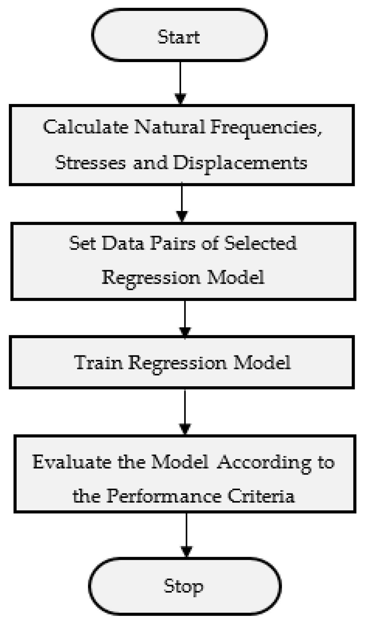
2.4. Regression Techniques Implemented

Regression, as denoted in the statistical literature, contains the prediction or learning of numeric features [30]. Regression holds significance across numerous engineering applications, as a multitude of real-world issues can be effectively addressed through the modeling of regression problems. Extensive research has been conducted in the field of maritime transportation [31,32,33].

Multiple regression (MR) is commonly used to investigate the causal relationship between multiple independent variables and a dependent variable simultaneously based on mathematical equations [34]. Each independent variable has its own coefficient, representing its unique contribution to the prediction of the dependent variable, while holding other variables constant. The algorithm calculates coefficients for the equation in a way that minimizes the sum of squared errors between the predicted values and the actual values [35]. The general mathematical form of multiple regression with “n” predictors is expressed as follows [36]:

$$y={\beta }_0+{\displaystyle \sum _{j=1}^m\left({\beta }_j{x}_j\right)}+\epsilon$$

(5)

Here, y is the dependent variable, x_j is an independent variable, β_j represents the regression coefficient associated with each regressor, β₀ is the constant term, and ε denotes the random error term.

The prediction accuracy of the regression model is investigated by performance metrics containing Coefficient of Determination (R²), Mean Square Error (MSE), and Mean Absolute Error (MAE).

The performance of all regression models is also investigated based on the Coefficient of Determination (R²) as given by the following expression:

$$R^2=1-\frac{{\displaystyle \sum _{i=1}^n{\left(predicte{d}_i-actua{l}_i\right)}^2}}{{\displaystyle \sum _{i=1}^n{\left(actua{l}_i-mean\left(actual\right)\right)}^2}}$$

(6)

R² measures the effectiveness of a model in fitting its data and presents variances in the measured variable. Its scale spans from 0 (indicating no explanatory power) to 1 (representing a perfect fit).

MSE determines the variations between predicted and actual values by averaging their squared disparities. Smaller values of MSE signify higher algorithm performance; however, it is susceptible to the influence of outliers [33].

$$MSE=\frac{1}{n}{\displaystyle \sum _{i=1}^n{\left(predicte{d}_i-actua{l}_i\right)}^2}$$

(7)

MAE evaluates the mean variation between predicted and actual values, treating all errors uniformly. It presents lower sensitivity to outlier data, rendering it advantageous in scenarios where substantial errors are undesirable [37].

$$MAE=\frac{1}{n}{\displaystyle \sum _{i=1}^n\left|predicte{d}_i-actua{l}_i\right|}$$

(8)

where the number of observations is represented by n. Within this manuscript, six main stages are used in the system architecture, as presented in Figure 4. These steps are assigned distinct and crucial responsibilities within the system.

3. Numerical Results and Discussions

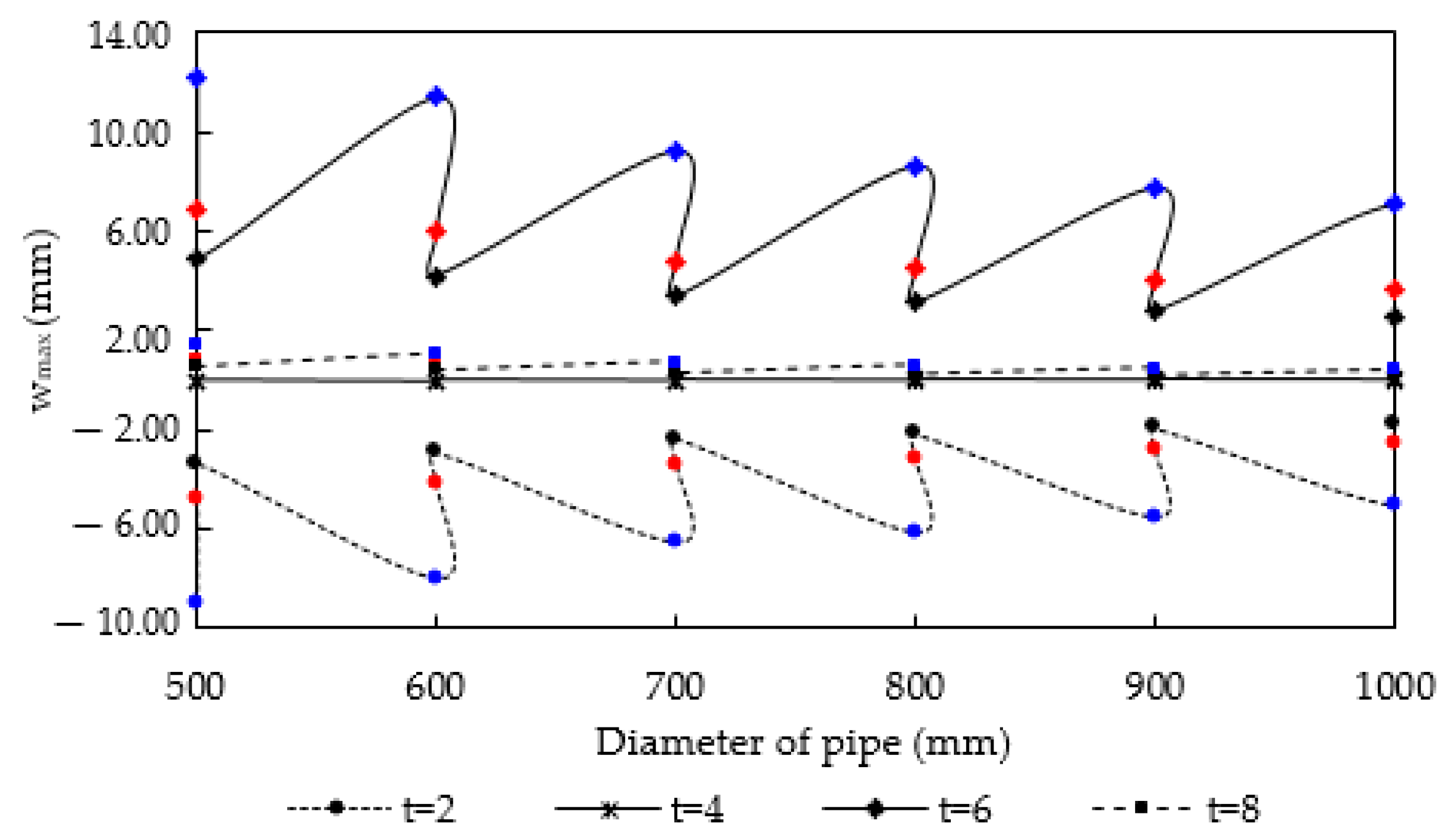
3.1. Natural Vibration Frequencies, Displacements, and Stresses of Pipeline Models

The analysis is conducted for a pipeline with a single opening and simple supported ends using the Euler–Bernoulli beam theory. The basis of the Euler–Bernoulli beam theory relies on three assumptions of continuum mechanics: first, that straight lines initially normal to the beam’s axis retain their straightness after deformation; second, that these lines are inextensible; and third, that they rotate as rigid lines perpendicular to the bent axis of the beam [38]. The axis x of the pipe is defined as a longer dimension, and the transverse vibration of the pipe that occurred on this axis is calculated.

The pipeline system’s dynamic performance can be described by identifying one or more natural vibration frequencies [39]. The high-frequency modes exhibit a more rapid decay in amplitude compared to the slower decay observed in the low-frequency modes. The dominant behavior is caused by the lower frequency modes [40]. Hence, the natural vibration frequencies of the pipe have been calculated for the first three modes in this study. Figure 5 shows the specific displacements required for the first three modes, initiating harmonic vibrations in the pipe.

The comparative results in

Table 2. Comparison of natural vibration frequency values.

D (mm)	tw (mm)	ω1 (Hz)	ω2 (Hz)	ω3 (Hz)
500	10	7.903	21.538	41.597
	20	7.750	21.128	40.833
	30	7.599	20.730	40.080
600	10	9.474	25.694	49.334
	20	9.322	25.297	48.591
	30	9.173	24.900	47.870
700	10	11.024	29.727	56.689
	20	10.906	29.343	55.991
	30	10.726	28.935	55.279
800	10	12.550	33.625	63.654
	20	12.402	33.256	62.972
	30	12.255	32.884	62.344
900	10	14.047	37.383	70.175
	20	13.902	37.023	69.589
	30	13.757	36.657	68.966
1000	10	15.516	40.984	86.993
	20	15.373	40.634	75.758
	30	15.230	40.290	75.131

present the obtained natural vibration frequency values from the analysis conducted for a single opening with simply supported ends of the pipeline.

In assessments where the internal flow in the pipe is neglected, it is observed that the natural vibration frequency values increase with an increase in the pipe diameter. Additionally, for each diameter, three different values of wall thickness also affect the frequency. It is evident that as the wall thickness increases, the results obtained for the same diameter decrease. The highest natural vibration frequency occurs when the wall diameter is 1000 mm and the wall thickness is 10 mm.

The maximum values of stress and displacement are used to create a dataset to explore relationships between variables for 18 pipe models. The maximum stress values contain the most significant strains occurring at the section where the maximum displacement is observed. The hydrodynamic forces vary depending on the velocity of fluid particles changing direction throughout the wave period. This leads to stresses calculated at the cross-section of the pipeline having different effects, with positive (+) and negative (−) pressures, as given in Figure 6. “BS EN 1993-1-1:2005+A1:2014 Eurocode 3. Design of steel structures General rules and rules for buildings” [41] and “BS EN 10025-2:2019 Hot rolled products of structural steels Technical delivery conditions for non-alloy structural steels” [42] are selected as steel standards in this study. The stress levels for all models remain within permissible limits.

The blue, red, and black colors represent the results for wall thicknesses of 10 mm, 20 mm, and 30 mm, respectively. As observed in the figure, results obtained at t = T/2, T/4, 3T/4, and T are compared. The stress values in the pipeline are highest at 2 s and 6 s, where wave crests and troughs occur, representing the peak hydrodynamic forces. An increase in wall thickness enhances strength, leading to a decrease in stress. However, the decrease in stress is not significant due to the increase in hydrodynamic force according to the Morison equation resulting from the increase in diameter. The maximum displacement that can occur in the cross-section of the pipeline is as crucial as stress. Particularly in systems where the gap between the pipeline and the seabed is small, erroneous calculations can lead to the deformation of the pipeline and significant financial losses [43]. Comparative results of maximum values are presented in Figure 7, considering the time intervals as t = T/2, T/4, 3T/4, and T.

Maximum displacements are observed again at the wave crest and trough positions. However, unlike stress values, it is evident that both the diameter and wall thickness values contribute to the decrease in displacement. Evaluating the scenario where displacement takes small values aims to ensure safety within the limits under the internal flow conditions, which will be considered in subsequent studies. The largest displacement, calculated as 0.113 mm, occurs at t = 6 s with D = 500 mm and t_w = 10 mm. The smallest value, 0.003 mm, is determined at t = 8 s when the surface profile returns to a calm sea surface, with D = 1000 mm and t = 30 mm. The relationship between datasets consisting of maximum stress and displacement values, independent of time, is presented in Figure 8.

It is observed that the relationship between maximum stress and displacement values is significant based on the Coefficient of Determination. Deviation in the values occurs when the hydrodynamic forces change from positive to negative. In this wave position, while stress increases, displacement values numerically decrease due to the change in direction.

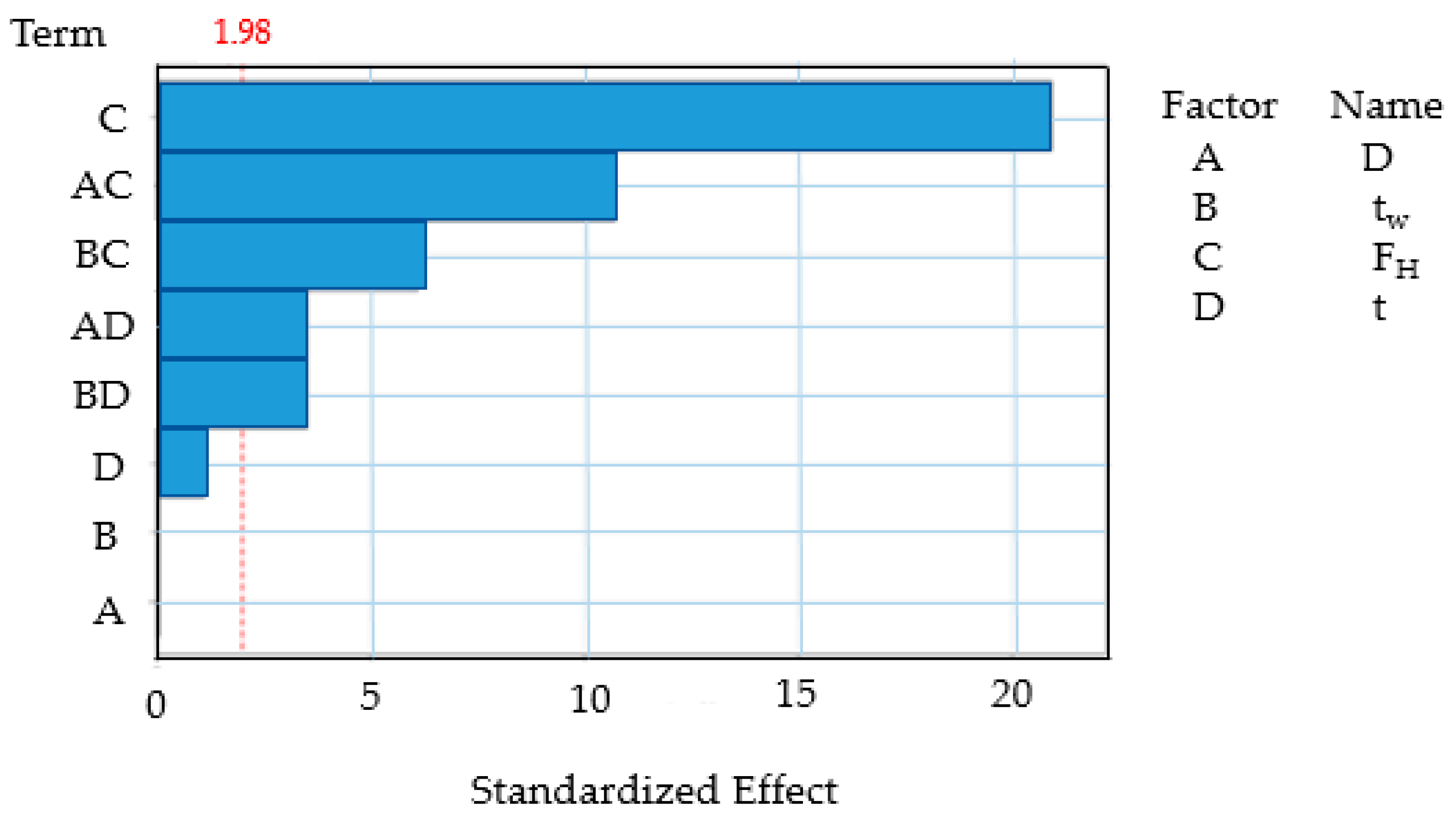
3.2. Comparative Results of Regression Models

In this section of this study, ANOVA (Analysis of Variance) results are generated. The effect magnitude of input parameters (D, t_w, FH, and t) on the outcomes (w_max, σ_max, ω₁, ω₂, and ω₃) is determined. Thus, the impact ratios of pipe diameter D, pipe wall thickness t_w, hydrodynamic force F_H, and time t are evaluated. In analyses where time is considered as input, the t/T approach is used to reach a general correlation. By using the dimensionless time term, the mathematical expression obtained ensures validity for wave models with different wave periods. Full quadratic models that include not only linear terms but also quadratic terms are developed for expressing more effective and concise mathematical equations [44]. The squares of the independent variables appear as part of the quadratic terms. These quadratic terms are included to capture nonlinear relationships between the predictor variables. It is expressed mathematically as follows:

Y = β₀ + β₁X₁ + β₂X₂ + β₃X₃ + … + β_kX_k + β₁₁X₁₂ + β₂₂X₂₂ + β₃₃X₃₂ + … + β_kk
X_k2 + β₁₂X₁X₂ + β₁₃X₁X₃ + … +β_(k−1)kX_(k−1)X_k+ε

(9)

where Y is the dependent variable, and X₁, X₂, X₃, …, X_k are the predictor variables. β₀, β₁, β₂, β₃, …, β_k are the coefficients for the linear terms; β₁₁, β₂₂, β₃₃, …, β_kk are the coefficients for the quadratic terms; β₁₂, β₁₃, …, β_(k−1)k are the coefficients for the interaction terms; and ε represents the error term.

Additionally, the effects of input parameters on the outcome parameters are demonstrated with 3D graphics.

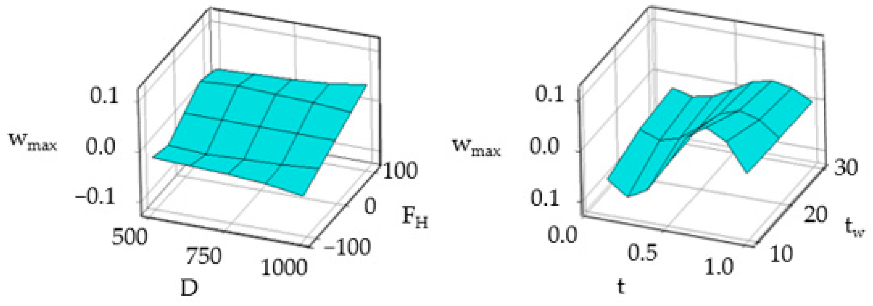
3.2.1. The Effect of Input Variables on Displacement Values

Displacement is an important parameter in the strength of the pipe. Knowing the extent to which each input affects displacement is of great importance. New mathematical models have been created using statistical methods to solve this problem in pipeline transportation systems. The results of the ANOVA analysis are provided in

Table 3. Analysis of Variance for w_max values.

Source	DF	Adj SS	Adj MS	F-Value	p-Value	%
D	1	0.000000	0.000000	0.00	0.969	0.000
tw	1	0.000000	0.000000	0.00	0.968	0.000
FH	1	0.072250	0.072250	438.81	0.000	29.476
t	1	0.000207	0.000207	1.26	0.264	0.084
D × FH	1	0.018939	0.018939	115.03	0.000	7.727
D × t	1	0.002039	0.002039	12.38	0.001	0.832
tw × FH	1	0.006155	0.006155	37.38	0.000	2.511
tw × t	1	0.002037	0.002037	12.37	0.001	0.831
Error	135	0.022228	0.000165			9.068
Total	143	0.245114				100.000

.

As seen in Table 3, within a 95% confidence interval, F_H, D × F_H, and t_w × F_H are the most influential parameters on the maximum displacement occurring throughout the independent period. At the same time frame, both the diameter and wall thickness of the pipe have a significant impact on displacement values. However, when a general regression model independent of time is constructed, hydrodynamic force and the conditions under which this parameter is multiplied become important.

The full quadratic model equation obtained using these parameters is given in Equation (10).

w_max = −0.0745 + 0.000061D + 0.001261t_w + 0.003184F_H + 0.1330t − 0.000002D ×
F_H − 0.000109D × t + 0.000022t_w × F_H − 0.002251t_w × T

(10)

F_H is the most influential parameter on maximum displacement, accounting for 29.476% of the effect. The effect ratio for D × F_H is 7.727%, while the effect ratio for t_w × F_H is 2.511%. The Pareto chart related to effective parameters is given in Figure 9.

The regression model achieves a high R² of 8.952 × 10⁻¹, which is close to the 1.0 perfect fit. Additionally, the model’s MSE value is 1.182 × 10⁻² and its MAE value is 8.081 × 10⁻². The results show that the model can accurately predict the maximum displacements of the pipeline. The relationship between maximum displacement values and input data is presented in Figure 10.

It is observed that hydrodynamic forces reach their maximum values under the crest and trough of the wave surface profile. When the hydrodynamic force is at its maximum, displacement values also increase. The increase in displacement values is more pronounced when the wall thickness is taken as 10 mm. Displacement values decrease as the pipe diameter increases. For the smallest selected diameter of 500 mm, the pipe experiences more oscillation due to the hydrodynamic force, resulting in a displacement change figure resembling the wave surface profile.

For the largest selected diameter of 1000 mm, the displacement values are maximum at the (−) and (+) maximum points of the hydrodynamic force, but the change curve reaches a more linear form. This indicates that increasing the pipe diameter and thickness reduces the destabilizing effect on stability in the transition regions of the hydrodynamic force causing tension and compression. The results obtained also highlight the importance of independent variable effect coefficients determined by ANOVA analysis in the design process.

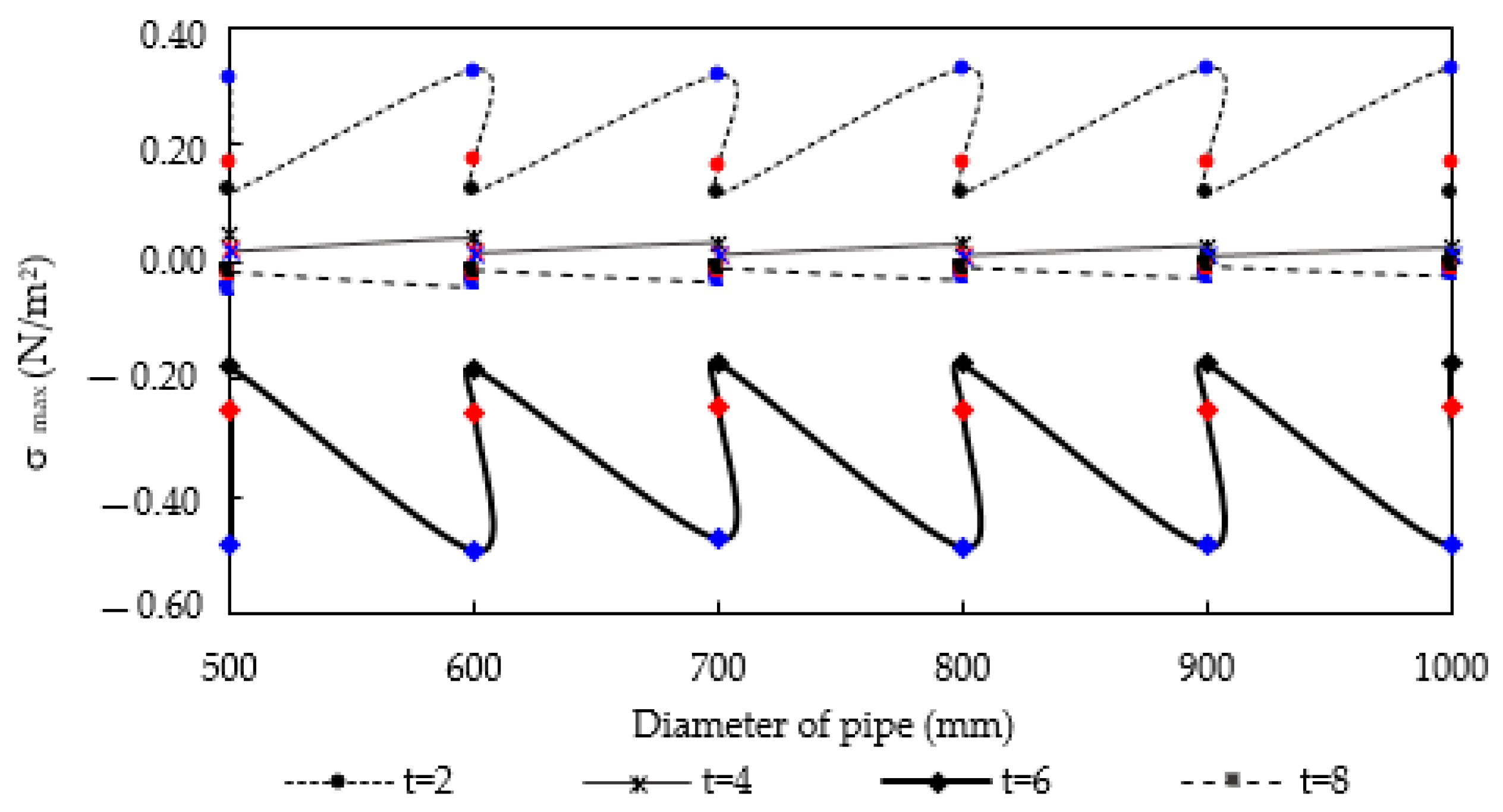
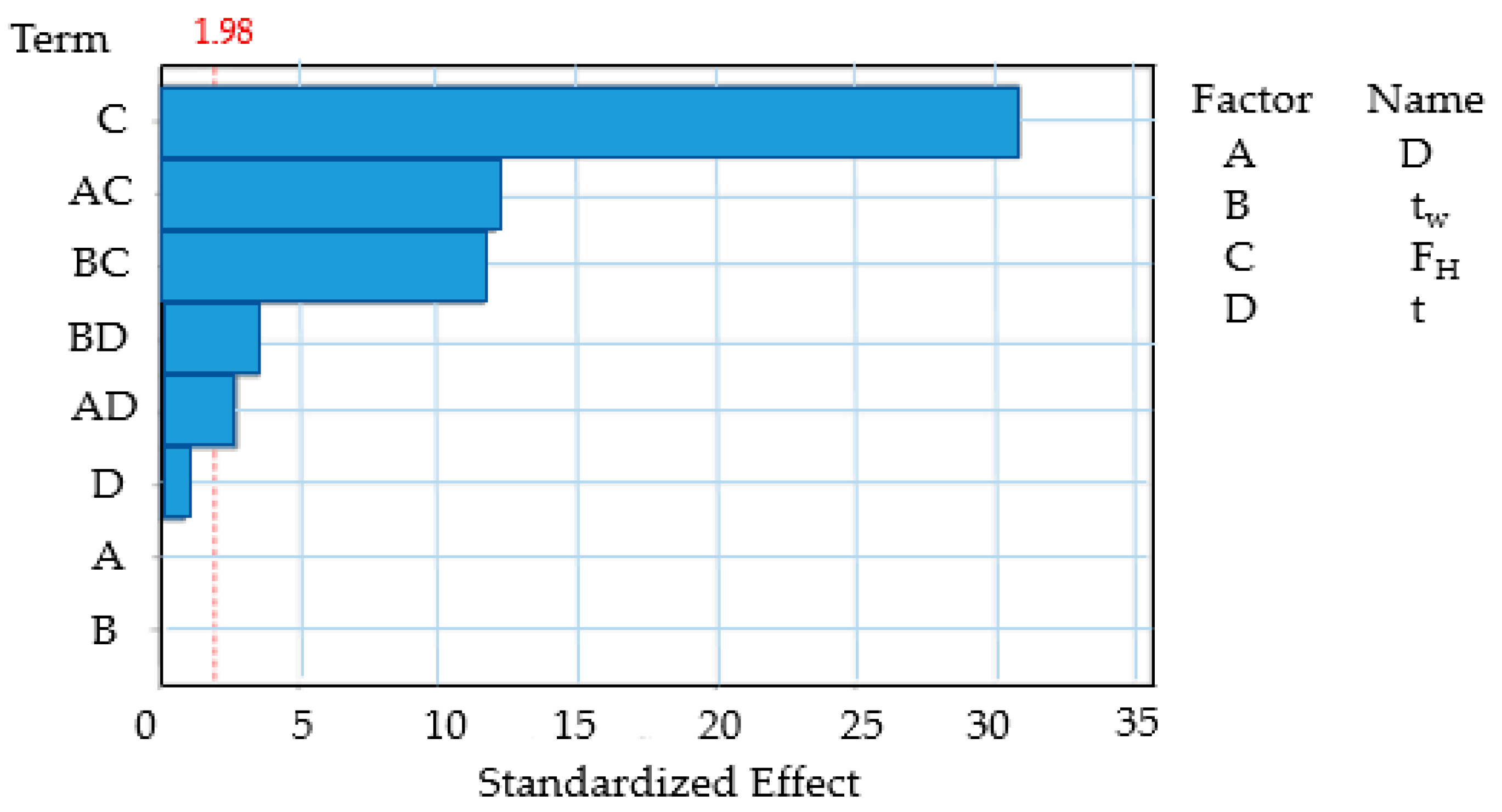
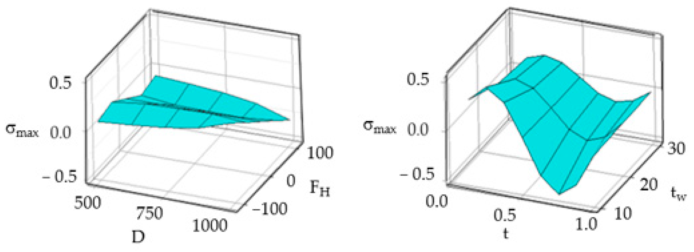
3.2.2. The Effect of Input Variables on Stress Values

Stress values serve as key indicators of the structural performance of submarine pipelines, and their proper evaluation and management are essential for ensuring the safety, reliability, and sustainability of these critical infrastructure systems [45]. The statistical analysis results, aimed at succinctly and practically illustrating the variation of this important parameter with respect to the geometric properties of the submarine pipeline, are presented in

Table 4. Analysis of Variance for σ_max values.

Source	DF	Adj SS	Adj MS	F-Value	p-Value	%
D	1	0.00000	0.00000	0.00	0.998	0.000
tw	1	0.00000	0.00000	0.00	0.998	0.000
FH	1	2.31716	2.31716	955.12	0.000	29.490
t	1	0.00206	0.00206	0.85	0.359	0.026
D × FH	1	0.35671	0.35671	147.04	0.000	4.540
D × t	1	0.01926	0.01926	7.94	0.006	0.245
tw × FH	1	0.33188	0.33188	136.80	0.000	4.224
tw × t	1	0.03215	0.03215	13.25	0.000	0.409
Error	135	0.32751	0.00243			4.168
Total	143	7.85733				100.000

.

As seen in Table 4, F_H is the most influential parameter on maximum stress values, accounting for 29.490% of the effect. The effect ratio for D × F_H is 4.540%, while the effect ratio for t_w × F_H is 4.224%. In the mathematical model, the properties of the pipeline are represented by 2-Way Interaction terms: D × F_H and t_w × F_H. The full quadratic model equation is presented in Equation (11).

σ_max = 0.2530 − 0.000188D − 0.00503tw − 0.016386FH − 0.450t + 0.000010D ×
FH + 0.000334D × t + 0.000164t_w × F_H + 0.00894t_w × t

(11)

The Pareto chart related to effective parameters is given in Figure 11.

The regression model exhibits a strong R² value of 9.518 × 10⁻¹, indicating that it explains a significant portion of the variance in the data. Moreover, MSE is low at 2.691 × 10⁻³ and MAE is 3.903 × 10⁻². The results of quality metrics showed that the model’s predictions are generally close to the actual values. The relationship between the independent variables and maximum stress is given in Figure 12.

The sudden changes in maximum stress values occurring under the wave crest and trough decrease with increasing diameter values. As the cross-sectional area of the pipeline increases, stability is enhanced, resulting in smaller oscillations in frequency. While the increase in pipe diameter leads to a higher hydrodynamic inertia force at t = 0, the resulting reductions in maximum stress values are relatively lower. However, over time, a significant decrease in stress becomes apparent.

The time-dependent maximum stress variation figure is obtained to be consistent with the water surface profile. The maximum stress values decrease with increasing wall thickness. The greatest difference between positive and negative stress values is obtained under the conditions of D = 500 and t_w = 10 mm. Significant variations in maximum tensile and compressive stresses can lead to fatigue of the pipeline over time and the occurrence of additional stresses.

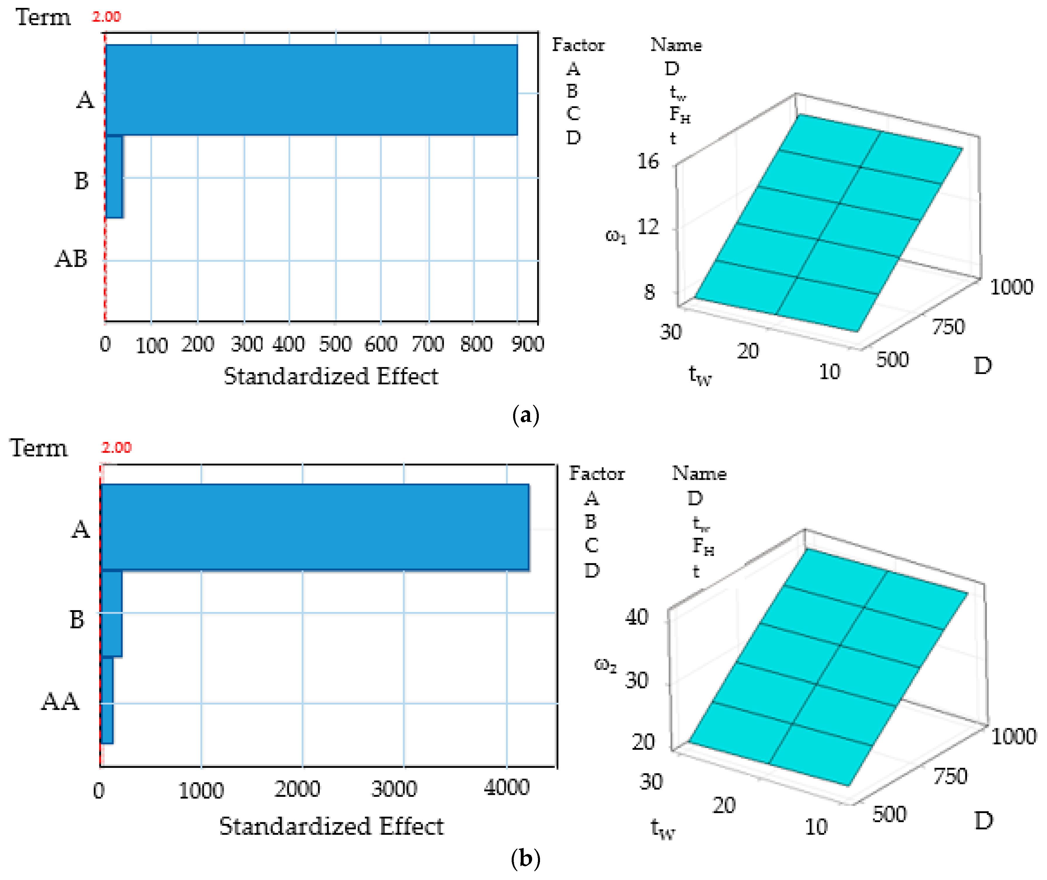
3.2.3. The Effect of Input Variables on Natural Vibration Frequencies

The natural vibration frequencies of submarine pipelines are essential considerations in ensuring their structural integrity and resilience against dynamic forces in underwater environments [46]. Hence, in this study, a variation analysis of the natural vibration frequencies for the initial three modes is conducted. The results of the Analysis of Variance (ANOVA) are presented in

Table 5. Analysis of Variance for ω₁, ω₂, and ω₃ values.

	Source	DF	Adj SS	Adj MS	F-Value	p-Value	%
ω1	D	1	976.437	976.437	795,364.29	0.000	99.768
	tw	1	2.098	2.098	1708.81	0.000	0.214
	D × t	1	0.001	0.001	0.72	0.397	0.000
	Error	140	0.172	0.001			0.018
	Total	143	978.708				100.000
ω2	D	1	6398.67	6398.670	17,918,183.400	0.000	99.718
	tw	1	13.82	13.820	38,706.740	0.000	0.215
	D × D	1	4.21	4.210	11,784.430	0.000	0.066
	Error	140	0.05	0.000			0.001
	Total	143	6416.75				100.000
ω3	D	1	26,667.7	26,667.700	2471.800	0.000	90.280
	tw	1	551.9	551.900	51.160	0.000	1.868
	D × D	1	154.3	154.300	14.300	0.000	0.522
	t × t	1	94.7	94.700	8.780	0.004	0.321
	D × t	1	581.3	581.300	53.880	0.000	1.968
	Error	138	1488.9	10.800			5.040
	Total	143	29,538.8				100.000

.

Typically, the lowest frequency mode, termed the first mode, is characterized by a uniform bending motion along the length of the pipeline. As seen in Table 5, the effect of D in the regression model is calculated as 99.768%, while the effect of t_w is computed as 0.214%. In contrast, the second mode presents a single-loop oscillation, resembling a half-wave pattern. Therefore, in addition to the effects of D at 99.718% and t_w at 0.215%, the term D × D also exhibits an effect of 0.066%. The third mode introduces an additional loop, leading to a more intricate vibration pattern. This also increases the number of terms required to define the mathematical model. In addition to D being the most effective parameter at 90.280% and t_w at 1.868%, the square (D × D, t_w × t_w) and 2-Way Interaction (D × t_w) parameters also gain importance.

The equations for the full quadratic model, obtained to describe the relationships between variables, are presented for the initial three natural vibration frequencies in Equations (12)–(14).

ω₁ = 0.4928 + 0.015212D − 0.01612t + 0.000002D × t

(12)

The model given by Equation (12) exhibits a strong R² value of 9.998 × 10⁻¹, indicating that it explains a significant portion of the variance in the data. Moreover, MSE is low at 1.207 × 10⁻³ and MAE is 2.849 × 10⁻².

ω₂ = −1.0575 + 0.049312D − 0.037945t − 0.000007D × D

(13)

The second vibration frequency model accounts for 100% of the variance in the dependent variable. It means that the model explains all the variability of the dependent variable around its mean using the independent variables. Additionally, both the MSE and MAE are low, recorded at 9.283 × 10⁻³ and 8.667 × 10⁻², respectively.

ω₃ = 11.39 + 0.0463D + 0.153t + 0.000041D × D + 0.01720t × t − 0.001441D × t

(14)

The model obtained using the third natural vibration frequency value exhibits a strong R² value of 9.437 × 10⁻¹, indicating that it explains a significant portion of the variance in the data. Even though defining the equation with more variables may decrease the actual prediction percentage, the results are within acceptable limits. The MSE value is determined to be 5.461, accompanied by a MAE value of 1.758.

The pareto charts, which are used to identify the most significant parameters for natural vibration frequencies, and 3D graphics are presented in Figure 13.

As seen in Figure 13, the geometry of the pipeline, including diameter and wall thickness, affects its natural vibration frequencies. Thicker pipelines tend to have lower frequency values. The effect of pipe thickness on natural vibration frequency increases with larger pipe diameters. Developing explicit expressions that define the relationship between the inputs and the natural vibration frequencies of the pipe would be particularly advantageous in terms of time and computational load, especially in the presence of internal flow.

Table 6. Performance comparison of the prediction equations.

Performance Criteria	Prediction Performance
R2	ω2 → ω1 → σmax → ω3 → wmax
MSE	ω1 → σmax → ω2 → wmax → ω3
MAE	ω1 → σmax → wmax→ ω2 → ω3

summarizes the previously obtained results, where the models are sorted in descending order, in terms of performance criteria, depending on the train data set used.

As seen in Table 6, the suggested equations for the full quadratic model exhibit the best performance for the initial two natural vibration frequencies. However, the relationship for displacement estimation, while remaining within the validity bounds, demonstrates weaker performance in terms of the R² value. The natural vibration frequency values for the third mode yield numerically larger results compared to other outputs. Therefore, MSE and MAE values are correspondingly larger.

4. Conclusions

The primary objective of this investigation is to establish the correlation among the factors influencing submarine pipelines without an extensive and complex analysis process. In this study, the widely used Airy Wave Theory is employed. Hydrodynamic wave forces acting on submarine pipeline models, each characterized by 18 different geometric properties, are calculated using the Morison Equation.

Dynamic behaviors are investigated through Finite Element-based computer-aided Time History analyses, with consideration given to constant clearance and environmental factors for each pipeline. A dataset including maximum displacement, stress, and the initial three natural vibration frequencies is generated. Multiple Regression analysis is performed using 144 data pairs with 4 inputs and 5 outputs. The relationship between inputs and outputs is defined by mathematical equations using a Full Quadratic model. Generally, it is observed that variations in diameter had a greater effect on displacement values than on stress values. The largest variation between predicted and actual values for maximum displacement and stress values occurs under conditions where the diameter is 1000 mm at T/4 and 3T/4. This finding supports the notion that hydrodynamic forces are the predominant variables in stress and displacement prediction equations. Examination of natural vibration frequency values reveals that increasing the number of variables required to describe the relationship between inputs and outputs reduced prediction performance by 5.630%. Therefore, this study aims to obtain the simplest mathematical equation possible, yielding the best results. Considering the influence of submarine pipeline geometry on hydrodynamic force variations, this study is significant in elucidating and interpreting the relationship between maximum stress, displacement, and natural vibration frequency. Furthermore, performance criteria are determined for each equation. These results show that the proposed models provide a highly accurate depiction of the data and give a great deal of confidence in the accuracy and reliability of the model. The results are observed in the case of neglecting the internal flow of the pipeline to simplify the analysis. When the internal flow of the pipeline is taken into account, correlations that include the effects on the outputs, especially on the natural vibration frequency, will become more significant. Future research will incorporate the effects of internal and external fluid flow. From this perspective, this study provides valuable insights into the underlying dynamics of submarine pipeline systems and analyzes inflection points in the relationships between variables.

References

1. Gong, S.W.; Lam, K.Y.; Lu, C. Structural analysis of a submarine pipeline subjected to underwater shock. Int. J. Press. Vessel. Pip. 2000, 77, 417–423. [Google Scholar] [CrossRef]
2. Yang, H.; Wang, A. Dynamic stability analysis of pipeline based on reliability using surrogate model. J. Mar. Eng. Technol. 2013, 12, 75–84. [Google Scholar]
3. Karampour, H.; Albermani, F.; Gross, J. On lateral and upheaval buckling of subsea pipelines. Eng. Struct. 2013, 52, 317–330. [Google Scholar] [CrossRef]
4. Chen, W.; Liu, C.; Li, Y.; Chen, G.; Jeng, D.; Liao, C.; Yu, J. An integrated numerical model for the stability of artificial submarine slope under wave load. Coast. Eng. 2020, 158, 103698. [Google Scholar] [CrossRef]
5. Hafez, K.A.; Abdelsalam, M.A.; Abdelhameed, A.N. Dynamic on-bottom stability analysis of subsea pipelines using finite element model-based general offshore analysis software: A case study. Beni-Suef Univ. J. Basic Appl. Sci. 2022, 11, 36. [Google Scholar] [CrossRef]
6. Meniconi, S.; Brunone, B.; Tirello, L.; Rubin, A.; Cifrodelli, M.; Capponi, C. Transient Tests for Checking the Trieste Subsea Pipeline: Toward Field Tests. J. Mar. Sci. Eng. 2024, 12, 374. [Google Scholar] [CrossRef]
7. Meniconi, S.; Brunone, B.; Tirello, L.; Rubin, A.; Cifrodelli, M.; Capponi, C. Transient Tests for Checking the Trieste Subsea Pipeline 2: Diving into Fault Detection. J. Mar. Sci. Eng. 2024, 12, 391. [Google Scholar] [CrossRef]
8. Youssef, B.S.; Cassidy, M.J.; Tian, Y. Application of statistical analysis techniques to pipeline on-bottom stability analysis. J. Offshore Mech. Arct. Eng. 2013, 135, 031701. [Google Scholar] [CrossRef]
9. Xu, H.; Sinha, S.K. A framework for statistical analysis of water pipeline field performance data. In Pipelines 2019; American Society of Civil Engineers: Reston, VA, USA, 2019; pp. 180–189. [Google Scholar]
10. Zhang, Y.; Weng, W.G. Bayesian network model for buried gas pipeline failure analysis caused by corrosion and external interference. Reliab. Eng. Syst. Saf. 2020, 203, 107089. [Google Scholar] [CrossRef]
11. Zhang, Y.; Wu, J.; Zhang, S.; Li, G.; Jeng, D.S.; Xu, J.; Tian, Z.; Xu, X. An optimal statistical regression model for predicting wave-induced equilibrium scour depth in sandy and silty seabeds beneath pipelines. Ocean. Eng. 2022, 258, 111709. [Google Scholar] [CrossRef]
12. Foo CS, X.; Liao, C.; Chen, J. Two-dimensional numerical study of seabed response around a buried pipeline under wave and current loading. J. Mar. Sci. Eng. 2019, 7, 66. [Google Scholar]
13. Guo, Z.; Hong, Y.; Jeng, D.S. Structure–Seabed Interactions in Marine Environments. J. Mar. Sci. Eng. 2021, 9, 972. [Google Scholar] [CrossRef]
14. Cohen, J.; Cohen, P.; West, S.G.; Aiken, L.S. Applied Multiple Regression/Correlation Analysis for the Behavioral Sciences; Routledge: London, UK, 2013. [Google Scholar]
15. Ducrozet, G.; Bouscasse, B.; Gouin, M.; Ferrant, P.; Bonnefoy, F. CN-Stream: Open-source library for nonlinear regular waves using stream function theory. arXiv 2019, arXiv:1901.10577. [Google Scholar]
16. Sarpkaya, T. Morison’s Equation and the Wave Forces on Offshore Structures; Naval Civil Engineering Laboratory: Carmel, CA, USA, 1981; p. 0270. [Google Scholar]
17. SAP 2000 V14 (Structural Analysis Program). Integrated Finite Element Analysis and Design of Structures; Computers and Structures Inc.: Berkeley, CA, USA, 2000. [Google Scholar]
18. Gücüyen, E. Numerical analysis of deteriorated sub-sea pipelines under environmental loads. Chin. J. Mech. Eng. 2015, 28, 1163–1170. [Google Scholar] [CrossRef]
19. Zhang, D.; Zhao, B.; Zhu, K. Dynamic Analysis of Pipeline Lifting Operations for Different Current Velocities and Wave Heights. FDMP-Fluid Dyn. Mater. Process. 2022, 19, 603–617. [Google Scholar] [CrossRef]
20. Reeve, D.; Chadwick, A.; Fleming, C. Coastal Engineering: Processes, Theory and Design Practice; CRC Press: Boca Raton, FL, USA, 2018. [Google Scholar]
21. Zhao, K.; Wang, Y.; Liu, P.L.F. A guide for selecting periodic water wave theories-Le Méhauté (1976)’s graph revisited. Coast. Eng. 2024, 188, 104432. [Google Scholar] [CrossRef]
22. Gücüyen, E.; Erdem, R.T.; Gökkuş, Ü. Irregular wave effects on dynamic behavior of piles. Arab. J. Sci. Eng. 2013, 38, 1047–1057. [Google Scholar] [CrossRef]
23. Airy, G.B. Tides and Waves; B. Fellowes: London, UK, 1845. [Google Scholar]
24. Chakrabarti, S. Handbook of Offshore Engineering (2-Volume Set); Elsevier: Amsterdam, The Netherlands, 2005. [Google Scholar]
25. Ahmadian, P. Effect of Hydrodynamic Forces on Spanning Pipes. Master’s Thesis, Eastern Mediterranean University (EMU)-Doğu Akdeniz Üniversitesi (DAÜ)), Gazimağusa, Cyprus, 2015. [Google Scholar]
26. Zan, X.; Lin, Z. On the applicability of Morison equation to force estimation induced by internal solitary wave on circular cylinder. Ocean. Eng. 2020, 198, 106966. [Google Scholar] [CrossRef]
27. Lin, W.; Su, C. An efficient Monte-Carlo simulation for the dynamic reliability analysis of jacket platforms subjected to random wave loads. J. Mar. Sci. Eng. 2021, 9, 380. [Google Scholar] [CrossRef]
28. Barltrop, N.D.P.; Adams, A.J. Dynamics of Fixed Marine Structures, 3rd ed.; Atkins Oil & Gas Engineering Limited: Epsom, UK, 1991. [Google Scholar]
29. Silwal, B. An Investigation of the Beam-Column and the Finite-Element Formulations for Analyzing Geometrically Nonlinear Thermal Response of Plane Frames. Master’s Thesis, Southern Illinois University, Carbondale, IL, USA, 2013. [Google Scholar]
30. Uysal, I.; Güvenir, H.A. An overview of regression techniques for knowledge discovery. Knowl. Eng. Rev. 1999, 14, 319–340. [Google Scholar] [CrossRef]
31. Ni, P.; Mangalathu, S.; Liu, K. Enhanced fragility analysis of buried pipelines through Lasso regression. Acta Geotech. 2020, 15, 471–487. [Google Scholar] [CrossRef]
32. Seghier, M.E.A.B.; Keshtegar, B.; Tee, K.F.; Zayed, T.; Abbassi, R.; Trung, N.T. Prediction of maximum pitting corrosion depth in oil and gas pipelines. Eng. Fail. Anal. 2020, 112, 104505. [Google Scholar] [CrossRef]
33. Banik, D.; Paul, R.; Rathore, R.S.; Jhaveri, R.H. Improved Regression Analysis with Ensemble Pipeline Approach for Applications across Multiple Domains. ACM Trans. Asian Low-Resour. Lang. Inf. Process. 2024, 23, 42. [Google Scholar] [CrossRef]
34. Dagli, B.Y.; Ergut, A.; Turan, M.E. Prediction of natural frequencies of Rayleigh pipe by hybrid meta-heuristic artificial neural network. J. Braz. Soc. Mech. Sci. Eng. 2023, 45, 221. [Google Scholar] [CrossRef]
35. Efendi, R.; Nawi, N.M.; Deris, M.M.; Burney, S.A. Cleansing of inconsistent sample in linear regression model based on rough sets theory. Syst. Soft Comput. 2023, 5, 200046. [Google Scholar]
36. Harle, S.M. Advancements and challenges in the application of artificial intelligence in civil engineering: A comprehensive review. Asian J. Civ. Eng. 2024, 25, 1061–1078. [Google Scholar] [CrossRef]
37. Fernandes, A.P.; Fonseca, A.; Pacheco, F.; Fernandes, L.S. Water quality predictions through linear regression-A brute force algorithm approach. MethodsX 2023, 10, 102153. [Google Scholar] [CrossRef] [PubMed]
38. Bauchau, O.A.; Craig, J.I. Euler-Bernoulli beam theory. In Structural Analysis; Springer: Dordrecht, The Netherlands, 2009; pp. 173–221. [Google Scholar]
39. Liu, M.; Wang, Z.; Zhou, Z.; Qu, Y.; Yu, Z.; Wei, Q.; Lu, L. Vibration response of multi-span fluid-conveying pipe with multiple accessories under complex boundary conditions. Eur. J. Mech. A/Solids 2018, 72, 41–56. [Google Scholar] [CrossRef]
40. Hou, R.; Xia, Y. Review on the new development of vibration-based damage identification for civil engineering structures: 2010–2019. J. Sound Vib. 2021, 491, 115741. [Google Scholar] [CrossRef]
41. BS EN 1993-1-1:2005+A1:2014; Eurocode 3-Design of Steel Structures: Part 1-1: General Rules and Rules for Buildings. BSI: London, UK, 1993.
42. BS EN 10025-2:2019; Hot Rolled Products of Structural Steels–Technical Delivery Conditions for Non-Alloy Structural Steels. BSI: London, UK, 2019.
43. Seghier ME, A.B.; Mustaffa, Z.; Zayed, T. Reliability assessment of subsea pipelines under the effect of spanning load and corrosion degradation. J. Nat. Gas Sci. Eng. 2022, 102, 104569. [Google Scholar] [CrossRef]
44. Bethea, R.M.; Rhinehart, R.R. Applied Engineering Statistics; Routledge: London, UK, 2019. [Google Scholar]
45. Revie, R.W. (Ed.) Oil and Gas Pipelines: Integrity and Safety Handbook; John Wiley & Sons: Hoboken, NJ, USA, 2015. [Google Scholar]
46. Hadi, N.; Helmi, M.; Cathaputra, E.; Priadi, D.; Dhaneswara, D. Freespan Analysis for Subsea Pipeline Integrity Management Strategy. J. Mater. Explor. Find. (JMEF) 2023, 1, 5. [Google Scholar]
Figure 1. Pipeline model.
Jmse 12 00955 g001
Figure 2. Surface elevations based on Airy Wave Theory.
Jmse 12 00955 g002
Figure 3. Time-varying hydrodynamic forces.
Jmse 12 00955 g003
Figure 4. Main steps of the system architecture.
Jmse 12 00955 g004
Figure 5. The initial mode shapes.
Jmse 12 00955 g005
Figure 6. Comparison of maximum values of stress.
Jmse 12 00955 g006
Figure 7. Comparison of maximum values of displacement.
Jmse 12 00955 g007
Figure 8. The maximum stress value versus the maximum displacement.
Jmse 12 00955 g008
Figure 9. Pareto chart of the standardized effects for wmax.
Jmse 12 00955 g009
Figure 10. Maximum displacement versus independent variables.
Jmse 12 00955 g010
Figure 11. Pareto chart of the standardized effects for σmax.
Jmse 12 00955 g011
Figure 12. Maximum stress versus independent variables.
Jmse 12 00955 g012
Figure 13. Pareto charts of the standardized effects for natural vibration frequencies and 3D graphics. (a) ω1, (b) ω2, and (c) ω3.
Jmse 12 00955 g013aJmse 12 00955 g013b