
Pursuing Optimization Using Multimodal Transportation System: A Strategic Approach to Minimizing Costs and CO2 Emissions

 ,
,  ,
,  ,
,  ,
,  and
and 
Abstract
1. Introduction
1.1. Contribution
1.2. Motivation
- What are the factors that influence the choice of transportation mode for cargo transshipment and temporary storage warehouses in the route from the south of the country to the ports of San Antonio and Valparaiso?
- How does the optimization model affect the costs and emissions associated with transshipment and temporary storage facilities along the route?
- What are the potential benefits and challenges of locating transshipment and temporary storage facilities in different locations?
2. Background
2.1. Description of System
2.2. Related Works
3. Materials and Methods
- Identify the research motivation, which is rooted in addressing a national logistics problem.
- Exploration of possible solutions to the problem and the decision to use a mathematical optimization model.
- Review and analyze various mathematical models, including the Capacitated Vehicle Routing Problem (CVRP) and discrete simulation, and compare how similar problems have been addressed in other regional contexts.
- Select the Hub and Spoke model as the most appropriate framework for this study.
- Collect freight data categorized by freight type and distances between cities and ports, with a focus on consolidating these data by freight type and mode.
- Conceptual design and development of the mathematical model, followed by its implementation using the GAMS programming language.
- Programming of several model formulations and iterative runs to derive the optimal solution.
- Analysis and discussion of the results, including further adjustments based on sensitivity analysis and additional calculations.
3.1. Optimization Modeling
3.1.1. Model Assumptions
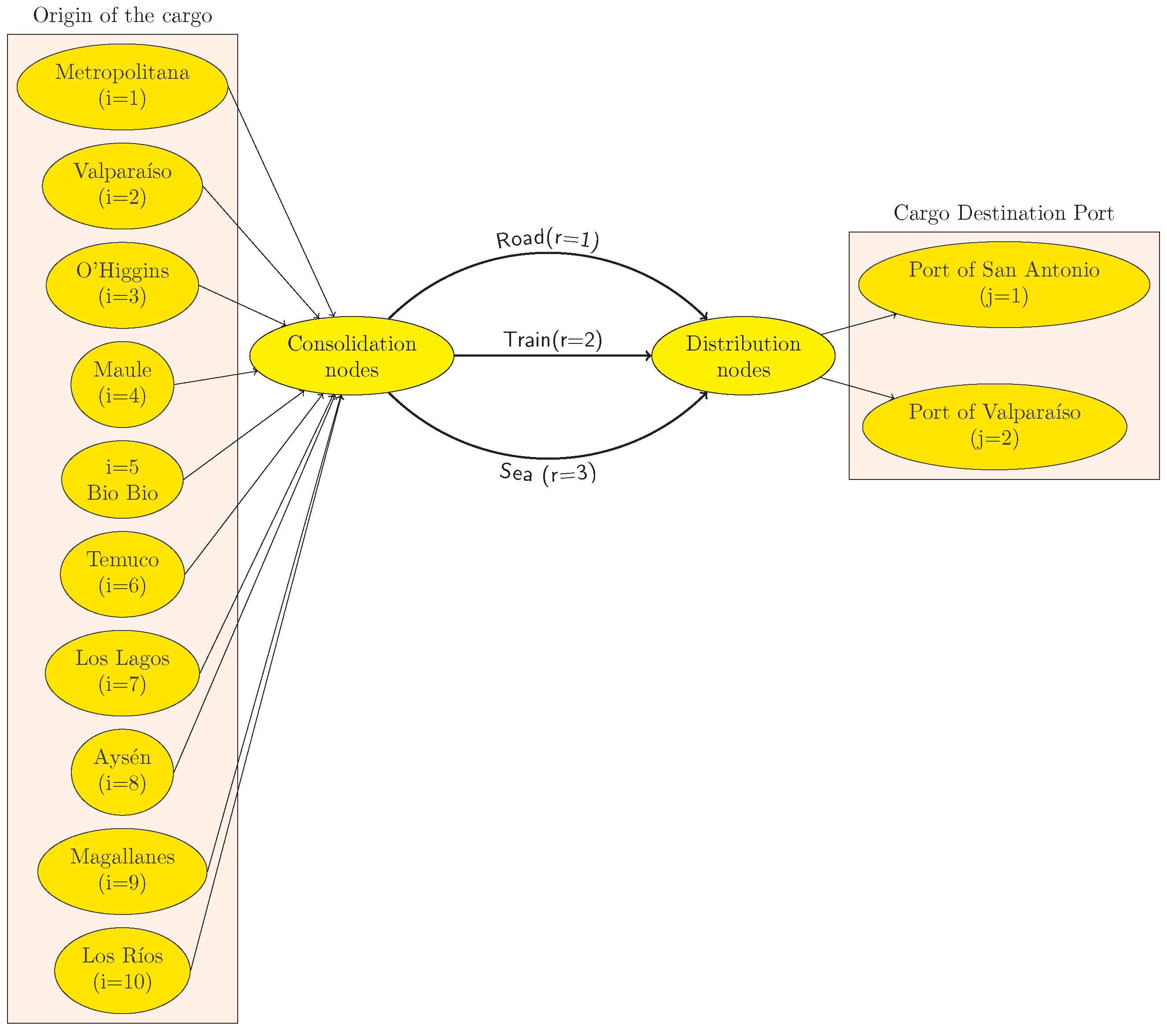
- Zones of origin of the load (index i):
- -
- Metropolitan Region, Santiago (i = 1),
- -
- Valparaíso Region, Valparaíso (i = 2),
- -
- O’Higgins Region, Rancagua (i = 3),
- -
- Maule Region, Talca (i = 4),
- -
- Bío Bío Region, Concepción (i = 5),
- -
- Temuco Region, Temuco (i = 6),
- -
- Los Lagos Region, Puerto Montt (i = 7),
- -
- General Carlos Ibáñez del Campo Region of Aysén, Coyhaique (i = 8),
- -
- Magallanes and Antarctica Chilen Region, Punta Arenas (i = 9)
- -
- Los Lagos Region, Valdivia (i = 10)
- Port cargo destination zones (index j):
- -
- San Antonio (j = 1),
- -
- Valparaíso (j = 2)
- Consolidation node installation zones (index k):
- -
- Metropolitana Region, Santiago (k = 1),
- -
- Valparaíso Region, Valparaíso (k = 2),
- -
- O’Higgins Region, Rancagua (k = 3),
- -
- Maule Region, Talca (k = 4),
- -
- Bío Bío Region, Concepción (k = 5),
- -
- Temuco Region, Temuco (k = 6),
- -
- Los Lagos Region, Puerto Montt (k = 7),
- -
- General Carlos Ibáñez del Campo Region of Aysén, Coyhaique Region (k = 8),
- -
- Magallanes and Antarctica Chilen Region, Punta Arenas (k = 9)
- -
- Los Lagos Region, Valdivia (k = 10)
- Distribution node zones (index m)
- -
- San Antonio (m = 1),
- -
- Zeal Zone of Valparaíso (m = 2),
- -
- Midpoint between San Antonio and Valparaíso (m = 3),
- -
- Calera (m = 4)
- Modes of transport (index r):
- -
- Road (r = 1),
- -
- Train (r = 2),
- -
- Ship (r = 3)
- Type of product (index p ):
- -
- General cargo (p = 1),
- -
- Refrigerated cargo (p = 2),
- -
- Liquid cargo (p = 3),
- -
- Bulk cargo (p = 4)
3.1.2. Objective Function
3.2. Data for the Chilean Multimodal System
3.2.1. Freight Transport Data: Distances and Volumes
3.2.2. Costs of Different Means of Transportation
3.2.3. Warehousing Costs
4. Results
5. Discussion and Conclusions
5.1. Limitations and Optimization Model
- Data Limitations: The applicability of the study is limited to the specific data used, particularly the load data at current rates, which are subject to annual variation.
- Data Availability and Accuracy: The data, such as cargo volumes reported by ports, is sourced from local customs and may contain errors due to regional processing discrepancies or data recording inconsistencies.
- Accuracy of Distance Measurements: Calculated origin-to-port distances are based on official records, which may not accurately reflect the actual routes taken by trucks or cargo, potentially leading to inaccuracies in distance-based analyses.
- Stakeholder Involvement: The study does not consider the involvement of key stakeholders, including local communities [59], in the development and implementation of the multimodal transportation system.
- Uncertainty Factors: The model does not account for uncertainties inherent in the transportation system, such as weather variations; accidents; or the overall volatility, uncertainty, complexity, and ambiguity [60] of the system.
5.2. Conclusions
5.3. Future Research
Author Contributions
Funding
Institutional Review Board Statement
Informed Consent Statement
Data Availability Statement
Acknowledgments
Conflicts of Interest
References
- Idowu, S.; Schmidpeter, R.; Capaldi, N.; Zu, L.; Del Baldo, M.; Abreu, R. (Eds.) CO2 Emissions in 2022; Springer: Cham, Switzerland, 2023; p. 600. [Google Scholar] [CrossRef]
- Li, H.; Wang, Y. Hierarchical Multimodal Hub Location Problem with Carbon Emissions. Sustainability 2023, 15, 1945. [Google Scholar] [CrossRef]
- Islam, D.M.Z.; Dinwoodie, J.; Roe, M. Promoting development through multimodal freight transport in Bangladesh. Transp. Rev. 2006, 26, 571–591. [Google Scholar] [CrossRef]
- Li, S.; Zu, Y.; Fang, H.; Liu, L.; Fan, T. Design Optimization of a HAZMAT Multimodal Hub-and-Spoke Network with Detour. Int. J. Environ. Res. Public Health 2021, 18, 12470. [Google Scholar] [CrossRef] [PubMed]
- Yin, C.Z.; Ke, Y.D.; Chen, J.H.; Liu, M. Interrelations between sea hub ports and inland hinterlands: Perspectives of multimodal freight transport organization and low carbon emissions. Ocean. Coast. Manag. 2021, 214, 105919. [Google Scholar] [CrossRef]
- Zheng, Y.; Ji, Y.; Shen, Y.; Liu, B.; Du, Y. Hub location problem considering spoke links with incentive-dependent capacities. Comput. Oper. Res. 2022, 148, 105959. [Google Scholar] [CrossRef]
- European Conference of Ministers of Transport. Transport Policy and Global Warming; University of Michigan: Ann Arbor, MI, USA, 1993; p. 241. [Google Scholar]
- Elbert, R.; Müller, J.P.; Rentschler, J. Tactical network planning and design in multimodal transportation—A systematic literature review. Res. Transp. Bus. Manag. 2020, 35, 100462. [Google Scholar] [CrossRef]
- Taran, I.; Olzhabayeva, R.; Oliskevych, M.; Danchuk, V. Structural Optimization of Multimodal Routes for Cargo Delivery. Arch. Transp. 2023, 67, 49–70. [Google Scholar] [CrossRef]
- Desrochers, M.; Lenstra, J.K.; Savelsbergh, M.W.P. A classification scheme for vehicle routing and scheduling problems. Eur. J. Oper. Res. 1990, 46, 322–332. [Google Scholar] [CrossRef]
- Ghoseiri, K.; Ghannadpour, S.F. Multi-objective vehicle routing problem with time windows using goal programming and genetic algorithm. Appl. Soft Comput. 2010, 10, 1096–1107. [Google Scholar] [CrossRef]
- Khoufi, I.; Laouiti, A.; Adjih, C. A Survey of Recent Extended Variants of the Traveling Salesman and Vehicle Routing Problems for Unmanned Aerial Vehicles. Drones 2019, 3, 66. [Google Scholar] [CrossRef]
- O’Kelly, M.E.; Campbell, J.F.; de Camargo, R.S.; de Miranda, G., Jr. Multiple Allocation Hub Location Model with Fixed Arc Costs. Geogr. Anal. 2015, 47, 73–96. [Google Scholar] [CrossRef]
- Zhang, H.; Liu, F.; Ma, L.; Zhang, Z. A Hybrid Heuristic Based on a Particle Swarm Algorithm to Solve the Capacitated Location-Routing Problem with Fuzzy Demands. IEEE Access 2020, 8, 153671–153691. [Google Scholar] [CrossRef]
- Hu, Y.; Zhang, K.; Yang, J.; Wu, Y. Application of Hierarchical Facility Location-Routing Problem with Optimization of an Underground Logistic System: A Case Study in China. Math. Probl. Eng. 2018, 2018, 7235048. [Google Scholar] [CrossRef]
- Zare Mehrjerdi, Y.; Nadizadeh, A. Using greedy clustering method to solve capacitated location-routing problem with fuzzy demands. Eur. J. Oper. Res. 2013, 229, 75–84. [Google Scholar] [CrossRef]
- Adi, T.N.; Bae, H.; Iskandar, Y.A. Interterminal Truck Routing Optimization Using Cooperative Multiagent Deep Reinforcement Learning. Processes 2021, 9, 1728. [Google Scholar] [CrossRef]
- Evangelista, D.G.D.; Vicerra, R.R.P.; Bandala, A.A. Approximate Optimization Model on Routing Sequence of Cargo Truck Operations through Manila Truck Routes using Genetic Algorithm. In Proceedings of the 2020 IEEE 12th International Conference on Humanoid, Nanotechnology, Information Technology, Communication and Control, Environment, and Management (HNICEM), Manila, Philippines, 3–7 December 2020; pp. 1–5. [Google Scholar] [CrossRef]
- Heilig, L.; Lalla-Ruiz, E.; Voss, S. Multi-objective inter-terminal truck routing. Transp. Res. Part E-Logist. Transp. Rev. 2017, 106, 178–202. [Google Scholar] [CrossRef]
- Karakas, S.; Kirmizi, M.; Kocaoglu, B. Yard block assignment, internal truck operations, and berth allocation in container terminals: Introducing carbon-footprint minimisation objectives. Marit. Econ. Logist. 2021, 23, 750–771. [Google Scholar] [CrossRef]
- O’Kelly, M.E. The Location of Interacting Hub Facilities. Transp. Sci. 1986, 20, 92–106. [Google Scholar] [CrossRef]
- The World Bank. Data: Logistics Performance Index: Overall (1=low to 5=high). 2023. Available online: https://data.worldbank.org/indicator/LP.LPI.OVRL.XQ (accessed on 21 December 2023).
- Dirección de Presupuestos: Ministerio de Hacienda. Indicadores de Desempeño 2023: Proyecto de Ley de Presupuestos 2023; Technical Report, Ministerio de Economía, Fomento y Turismo; Corporación de Fomento de la Producción: Santiago, Chile, 2022. [Google Scholar]
- Corporación de Fomento de la Producción. Programas Estratégicos Integrados; Corporación de Fomento de la Producción: Santiago, Chile, 2024. [Google Scholar]
- Delbeke, J.; Vis, P. (Eds.) EU Climate Policy Explained; Routledge: New York, NY, USA, 2015; p. 152. [Google Scholar]
- Liu, S. Multimodal Transportation Route Optimization of Cold Chain Container in Time-Varying Network Considering Carbon Emissions. Sustainability 2023, 15, 4435. [Google Scholar] [CrossRef]
- Camara Maritima y Portuaría de Chile, A.G. Análisis Comparativo Comercio Exterior: Enero–Diciembre 2023 vs. 2022; Technical Report; Camara Maritima y Portuaría de Chile A.G.: Valparaíso, Chile, 2024. [Google Scholar]
- Subdirección de Desarrollo. Red Vial Nacional: Dimensionamiento y Características; Technical Report; Dirección de Vialidad, MOP: Santiago, Chile, 2023. [Google Scholar]
- Programa de Desarrollo Logístico—Subsecretaría de Transportes; Ministerio de Transportes y Telecomunicaciones; Ministerio de Economía, Fomento y Turismo. Política Nacional Logística-Portuaria: Consolidado de Diagnósticos y Propuestas; Technical Report; Programa de Desarrollo Logístico—Subsecretaría de Transportes: Santiago, Chile, 2023. [Google Scholar]
- SEP. Informe Financiero a Marzo 2023; Technical Report; Ministerio de Economía, Fomento y Turismo, Gobierno de Chile: Santiago, Chile, 2023. [Google Scholar]
- CORFO. Información Complementaria: Desafíos de Innovación e I+D Empresarial Para Sectores Estratégicos de alto Impacto; Technical Report; CORFO, Gobierno de Chile: Santiago, Chile, 2017. [Google Scholar]
- Subsecretaria de Relaciones Económicas Internacionales de Chile. Comercio exterior de Chile crece 21% y supera los USD104.000 millones en el 2022. 2022. Available online: https://www.legiscomex.com/es/comercio-exterior-de-chile-crece-21-y-supera-los-usd104000-millones-en-el-2022 (accessed on 25 March 2024).
- Behdani, B.; Fan, Y.; Wiegmans, B.; Zuidwijk, R. Multimodal schedule design for synchromodal freight transport systems. Eur. J. Transp. Infrastruct. Res. 2016, 16, 424–444. [Google Scholar] [CrossRef]
- Zhang, M.; Pel, A.J. Synchromodal hinterland freight transport: Model study for the port of Rotterdam. J. Transp. Geogr. 2016, 52, 1–10. [Google Scholar] [CrossRef]
- Okyere, S.; Yang, J.Q.; Adams, C.A. Optimizing the Sustainable Multimodal Freight Transport and Logistics System Based on the Genetic Algorithm. Sustainability 2022, 14, 11577. [Google Scholar] [CrossRef]
- Kotikov, J. Geographic information system modelling of freight transport and logistics in Saint Petersburg, Russia. Proc. Inst. Civ.-Eng.-Civ. Eng. 2015, 168, 31–38. [Google Scholar] [CrossRef]
- Batarliene, N.; Sakalys, R. Mathematical Model for Cargo Allocation Problem in Synchromodal Transportation. Symmetry 2021, 13, 540. [Google Scholar] [CrossRef]
- Chang, Z.; Weng, J.X.; Qi, Z.; Yang, D. Assess economic and environmental trade-off for inland port location. Int. J. Shipp. Transp. Logist. 2019, 11, 243–261. [Google Scholar] [CrossRef]
- Zhang, J.R.; Zhang, S.J.; Wang, Y.J.; Bao, S.H.; Yang, D.Y.; Xu, H.L.; Wu, R.; Wang, R.J.; Yan, M.; Wu, Y.; et al. Air quality improvement via modal shift: Assessment of rail-water-port integrated system planning in Shenzhen, China. Sci. Total. Environ. 2021, 791, 148158. [Google Scholar] [CrossRef] [PubMed]
- Zhang, W.P.; Wu, X.H.; Guo, J. CO2 Emission Efficiency Analysis of Rail-Water Intermodal Transport: A Novel Network DEA Model. J. Mar. Sci. Eng. 2022, 10, 1200. [Google Scholar] [CrossRef]
- Kim, N.S.; Janic, M.; van Wee, B. Trade-Off Between Carbon Dioxide Emissions and Logistics Costs Based on Multiobjective Optimization. Transp. Res. Rec. 2009, 2139, 107–116. [Google Scholar] [CrossRef]
- Yin, C.Z.; Lu, Y.; Xu, X.F.; Tao, X.Z. Railway freight subsidy mechanism based on multimodal transportation. Transp.-Lett.- Int. J. Transp. Res. 2021, 13, 716–727. [Google Scholar] [CrossRef]
- Rodrigues, V.S.; Pettit, S.; Harris, I.; Beresford, A.; Piecyk, M.; Yang, Z.; Ng, A. UK supply chain carbon mitigation strategies using alternative ports and multimodal freight transport operations. Transp. Res. Part -Logist. Transp. Rev. 2015, 78, 40–56. [Google Scholar] [CrossRef]
- Santos, T.A.; dos Santos, G.L.; Martins, P.; Soares, C.G. A methodology for short-sea-shipping service design within intermodal transport chains. Marit. Econ. Logist. 2022, 24, 138–167. [Google Scholar] [CrossRef]
- Yamaguchi, T.; Shibasaki, R.; Samizo, H.; Ushirooka, H. Impact on Myanmar’s Logistics Flow of the East-West and Southern Corridor Development of the Greater Mekong Subregion-A Global Logistics Intermodal Network Simulation. Sustainability 2021, 13, 668. [Google Scholar] [CrossRef]
- Gumuskaya, V.; van Jaarsveld, W.; Dijkman, R.; Grefen, P.; Veenstra, A. Dynamic barge planning with stochastic container arrivals. Transp. Res. Part E-Logist. Transp. Rev. 2020, 144, 102161. [Google Scholar] [CrossRef]
- Iannone, F. The private and social cost efficiency of port hinterland container distribution through a regional logistics system. Transp. Res. Part A-Policy Pract. 2012, 46, 1424–1448. [Google Scholar] [CrossRef]
- Dini, N.; Yaghoubi, S.; Bahrami, H. Route selection of periodic multimodal transport for logistics company: An optimisation approach. Res. Transp. Bus. Manag. 2024, 54, 101123. [Google Scholar] [CrossRef]
- Yang, J.; Liang, D.; Zhang, Z.; Wang, H.; Bin, H. Path Optimization of Container Multimodal Transportation Considering Differences in Cargo Time Sensitivity. Transp. Res. Rec. 2024, 03611981241243077. [Google Scholar] [CrossRef]
- Hu, X.; Cheng, R.; Zhao, J.; Wang, R.; Zhang, T.; Lei, H.; Liu, B. Promotion strategy of low-carbon multimodal transportation considering government regulation and cargo owners’ willingness. In Environment, Development and Sustainability; Springer: Berlin/Heidelberg, Germany, 2024. [Google Scholar] [CrossRef]
- Ge, J.; Sun, Y. Solving a Multimodal Routing Problem with Pickup and Delivery Time Windows under LR Triangular Fuzzy Capacity Constraints. Axioms 2024, 13, 220. [Google Scholar] [CrossRef]
- Dirección Nacional de Aduanas. Base de datos Operaciones de Ingreso. 2023. Available online: https://www.aduana.cl/base-de-datos-operaciones-de-ingreso/aduana/2018-12-28/102736.html (accessed on 27 November 2023).
- Cámara de Comercio de Santiago. Costos de Transporte de Importaciones Profundizó su caída en el Primer Trimestre. 2023. Available online: https://www.ccs.cl/2023/07/20/costos-de-transporte-de-importaciones-profundizo-su-caida-en-el-primer-trimestre/ (accessed on 26 March 2023).
- Steer. Actualización de Modelo de Costos de Transporte de Carga para el Análisis de Costos Logísticos, del Observatorio Logístico; Technical Report; Subsecretaría de Transportes: Santiago, Chile, 2020. [Google Scholar]
- Puertos & Logistica. Memoria Anual 2017 Puertos & Logistica; Technical Report; Puertos & Logistica: Santiago, Chile, 2017. [Google Scholar]
- GAMS Development Corp. The General Algebraic Modeling Language, version GAMS 46.3.0; GAMS Development Corp: Fairfax, VA, USA, 2024. [Google Scholar]
- Zuse Institute Berlin. SCIP: Solving Constraint Integer Programs; Version 9.0.0; Zuse Institute Berlin: Berlin, Germany, 2024. [Google Scholar]
- Pettigrew, S.; Delgado, O.; Pineda, L.; Khan, T.; Rebouças, A.B.; Yang, Z.; Vera, M.; Gardner, G.; Gordillo, J. Fuel Economy Standards and Zero-Emission Vehicle Targets in Chile; Technical Report August 2022; International Council on Clean Transportation: Washington, DC, USA, 2022. [Google Scholar]
- Durán, C.; Fernández-Campusano, C.; Carrasco, R.; Vargas, M.; Navarrete, A. Boosting the Decision-Making in Smart Ports by using Blockchain. IEEE Access 2021, 9, 128055–128068. [Google Scholar] [CrossRef]
- Fuentealba, D.; Flores-Fernández, C.; Carrasco, R. Análisis bibliométrico y de contenido sobre VUCA. Rev. Esp. Doc. Cient. 2023, 46, e354. [Google Scholar] [CrossRef]
- O’Kelly, M.E.; Miller, H.J. The hub network design problem: A review and synthesis. J. Transp. Geogr. 1994, 2, 31–40. [Google Scholar] [CrossRef]
- Ernst, A.T.; Krishnamoorthy, M. Efficient algorithms for the uncapacitated single allocation p-hub median problem. Locat. Sci. 1996, 4, 139–154. [Google Scholar] [CrossRef]
- F & K Consultores. Análisis de Precios del Transporte Ferroviario en Algunas de las Cadenas Logísticas Contenidas en el Plan de Impulso a la Carga Ferroviaria (Picaf), en vías de Propiedad de la Empresa de los Ferrocarriles del Estado; F & K Consultores: Santiago, Chile, 2015. [Google Scholar]
- Janic, M.; Vleugel, J. Estimating potential reductions in externalities from rail–road substitution in Trans-European freight transport corridors. Transp. Res. Part D Transp. Environ. 2012, 17, 154–160. [Google Scholar] [CrossRef]
- Ministerio de Transportes y Telecomunicaciones; Subsecretaria de Transportes. Plan de Impulso a la Carga Ferroviaria; Ministerio de Transportes y Telecomunicaciones: Santiago, Chile, 2014; Volume 3B, p. 43. [Google Scholar]
- Mallat Garcés, G. Chile y los corredores bioceánicos—Santo Tomás en Línea. 2023. Available online: https://enlinea.santotomas.cl/blog-expertos/chile-y-los-corredores-bioceanicos/ (accessed on 27 March 2024).


| Author | Method/Model/Technique | Limitations | Contributions |
|---|---|---|---|
| Transport industry: | |||
| [5] | Multi-objective planning model | Exploring model applicability in various regions, incorporating diverse transport modes, and managing dynamic supply chain and logistics uncertainties are essential areas for research. | Rail transport is the most efficient mode for long distances, surpassing other methods in terms of cost and carbon emissions. |
| [33] | Mathematical modeling to design service schedules for synchromodal freight transport systems. | Examines a case of the Port of Rotterdam hinterland network, limiting generalizability. The study lacks information on barriers to synchromodal freight transport systems. | Improved performance of the intermodal freight system, achieving cost savings equivalent to a reduction of more than 20%. |
| [34] | SynchroMO algorithm | The study of the Port of Rotterdam hinterland network could limit the results’ relevance. Analysis is required for infrastructure, stakeholder collaboration, and regulations. | It allows simulations and comparisons to be made between different routes and schedules, depending on the goods transiting the Rotterdam hinterland container transport. |
| [35] | Genetic algorithm | The study examines 10 regional capitals in Ghana, limiting generalizability. The genetic algorithm model considers time, distance, and CO2 emissions but overlooks other sustainability factors. | By optimizing the system, total cost savings were achieved, representing a reduction of 4.5% compared to the same amount of cargo transported with the traditional system. |
| [36] | ArcGIS and event model | The research centers on GIS modeling of freight transportation and logistics in Russia. It does not mention the specific event model employed or the constraints of the GIS model. The absence of exploration into potential biases of the data utilized. | Optimizes the planning and coordination of the transportation and logistics system in the city of St. Petersburg, thus improving regional connectivity within Europe. |
| [37] | Stochastic integer programming model | The paper presents an optimization model for load allocation in synchromodal transport but lacks detailed information on solution techniques, focuses on a specific problem, and lacks assumptions in the model. | Improves sustainability, increases flexibility, and reduces costs, among other benefits, in the field of freight transportation. |
| [38] | Multi-objective optimization and genetic algorithm | The investigation focuses on transportation cost, fixed cost, and CO2 emissions while overlooking social impacts, land use, and noise pollution factors. Challenges and limitations in applying the model for real-world decisions are not analyzed. | Inland ports are positioned in a multimodal freight transport network to optimize transport and operational costs while lowering CO2 emissions. The growth of inland ports is linked to cost and emission reductions. |
| [39] | Multimodal environment evaluation tool (MEET) | The study examines how modal shifts in Shenzhen affect air quality without considering social impacts, land use changes, or noise pollution. More research is required to assess the success of accompanying strategies and measure extra advantages. | Replacing road transport with sustainable options such as rail and river transport can benefit port cities in terms of transport efficiency and environmental quality. Stricter emission standards for vehicles can improve air quality by reducing NOX and O3 levels. |
| [40] | Data envelopment analysis (DEA) model | The research explores carbon emissions efficiency of rail–water intermodal transport in China, but findings may not be generalizable. It concentrates on CO2 emissions and overlooks other environmental impacts or pollutants. | Evaluates the carbon emission efficiency of rail–water intermodal transport in 14 Chinese ports, facilitating sustainable transport planning and decision making. |
| [41] | Multi-objective optimization | The research on a European port freight transport network may limit generalizability. Other factors like infrastructural constraints and regulatory policies could affect CO2 emissions and logistics costs balance. | Examines the relationship between logistics costs and CO2 emissions in various freight transport networks. Evaluates the effects of changing modes and routes on the balance between costs and emissions, emphasizing the role of the demands and capacities of the freight transport system. |
| [42] | Integrates Dijkstra’s algorithm and a pattern search algorithm in a bi-level programming model | It is necessary to examine the risks of implementing the subsidy mechanism in the various transport and logistics planning modes. Further analysis is required to understand the proposal’s economic, social, environmental, and political effects. | Utilizes Yangtze River data to optimize China Railway Express freight subsidy system in multimodal transportation setup, improving decision-making and policy development for sustainable transport. Sets specific intervals for adjusting unit subsidy based on the transported cargo type. |
| Industria Portuaria | |||
| [43] | Linear optimization | An in-depth examination of transport strategies, associated risks, and subsidy mechanisms implications is needed. Real-world uncertainties like personnel performance in port operations and current regulations must be evaluated. | Examines carbon reduction methods in supply chains of London Gateway, studying alternative ports and transport modes like short sea shipping. Decreasing travel distances and CO2 e emissions leads to lower costs. |
| [44] | Logistic regression model | The logistic regression model of the case study needs to study service reliability and environmental impact to improve the effectiveness of the service design. | Optimizing SSS services in intermodal transport chains involves designing the optimal vessel size based on demand estimation. A case study of a Ro-Pax service in Portugal shows how design adjustments can improve economic performance. |
| [45] | Stochastic network assignment model and global logistics intermodal network simulation model | The model neglects external factors like politics or economics affecting logistics flow. Simulation results are restricted by data availability and accuracy for comparison with observed flows. | Evaluates logistics infrastructure policies in the Greater Mekong subregion of Myanmar and tests various scenarios to determine their effects on goods movement and container traffic. Analyzes the environmental and economic impact of increased truck speed and the opening of the Dawei port on transport modes. |
| [46] | Two-stage stochastic mixed integer model (MIP) | Lack of consideration of weather conditions, port congestion, and labor availability, which affects throughput and operating costs. More accurate costing is required for various scenarios and terminals. | Examines how uncertainty affects barge transportation by analyzing real data from a land terminal and evaluating long-term performance through simulated weekly operations for one year. Creates a stochastic program for transportation planning that demonstrates that uncertainty can influence total costs. |
| [47] | Interport Model (network programming tool) | The model examines the rationality of economic agents and perfect competition. Studying the uncertainty of factors such as container demand, costs, capacity constraints, and regulatory changes is convenient. | Investigates the link between sustainability and container logistics in Campania ports. Examines the impact of policies and measures on the competitiveness and sustainability of container distribution. Emphasizes the reduction of transport costs and suggests public and private strategies for green transport. |
| Symbol | Description |
|---|---|
| Transport of cargo from origin node i to port of embarkation j for product type p. | |
| Unit cost of transport from the origin node i to the consolidation node k for product type p along route r [dollars per ton-kilometer]. | |
| Unit transport cost from consolidation node k to distribution node m for product type p on route r [dollars per ton-kilometer]. | |
| Unit cost of transportation between distribution node m and port j for product type p along route r [dollars per ton-kilometer] | |
| Unit transport cost from origin node i to consolidation node m for product type p via the route. | |
| Unit transport cost from origin node i to consolidation node m for product type p via the route r. | |
| Unit cost of transportation between node i and port of embarkation j for product p and route r. | |
| Generic expression for the distance between the origin node i and the consolidation center at node k. | |
| Generic expression for the distance from consolidation center k to destination node j. | |
| Generic expression for the distance from consolidation center m to destination node j. | |
| Generic expression for the distance between the consolidation center k and the distribution center at node m. | |
| Investment for the setup, operation, and maintenance of a consolidation node. | |
| Investment for the setup, operation, and maintenance of a distribution node. | |
| a | Project evaluation period. |
| Symbol | Description |
|---|---|
| A binary variable that equals 1 if product type p is shipped directly from origin i to destination j via route r, and 0 otherwise. | |
| Binary variable is 1 if transport is from origin i to node k for product type p via route r, and 0 otherwise. | |
| Binary variable equals 1 if cargo is transported from node k to j for product type p along route r, and 0 otherwise. | |
| Binary variable is 1 if cargo moves from consolidation node k to distribution node m for product type p via route r, and otherwise 0. | |
| Binary variable equal to 1 if the cargo is transported from node m to port j for product type p via route r, and 0 otherwise. | |
| Binary variable is 1 if cargo is transported from node k to port j for product type p via route r, and 0 otherwise. | |
| Binary variable that is 1 if a consolidation node is installed at node k, and 0 otherwise. | |
| Binary variable is 1 if a distribution node is installed at node m, and 0 otherwise. | |
| Binary variable: 1 if no consolidation or distribution nodes are installed, and 0 otherwise. | |
| Binary variable set to 1 for installing consolidation node at node k and distribution node at node m, and 0 otherwise. | |
| A binary variable indicating 1 for a distribution node installation at node m, and 0 otherwise. | |
| Binary variable equal to 1 if a consolidation node is installed at node k, and 0 otherwise. |
| ID | Region, Capital City | General | Refrigerated | Liquid | Granel |
|---|---|---|---|---|---|
| 1 | Metropolitan Region, Santiago | 7,543,212 | 640,633 | 15,897 | 17,683 |
| 2 | Valparaíso Region, Valparaíso | 880,155 | 1,153,233 | 19,576 | 0 |
| 3 | O’Higgins Region, Rancagua | 1,491,447 | 3,949,870 | 6456 | 0 |
| 4 | Maule Region, Talca | 2,457,589 | 1,545,269 | 22,395 | 0 |
| 5 | Bío Bío Region, Concepción | 320,855 | 48,966 | 144 | 179,314 |
| 6 | Temuco Region, Temuco | 4345 | 58,460 | 0 | 0 |
| 7 | Los Lagos Region, Puerto Montt | 27,845 | 48,016 | 0 | 0 |
| 8 | General Carlos Ibáñez del Campo Region of Aysén, Coyhaique | 8914 | 60,266 | 0 | 0 |
| 9 | Magallanes and Antarctica Chilen Region | 38,078 | 210,935 | 0 | 0 |
| 10 | Los Ríos Region, Valdivia | 24,358 | 12,794 | 0 | 0 |
| ID | Region, Capital City | General | Refrigerated | Liquid | Granel |
|---|---|---|---|---|---|
| 1 | Metropolitan Region, Santiago | 4,133,243 | 530,133 | 6408 | 1 |
| 2 | Valparaíso Region, Valparaíso | 773,020 | 991,239 | 67,241 | 0 |
| 3 | O’Higgins Region, Rancagua | 673,554 | 3,208,655 | 2836 | 0 |
| 4 | Maule Region, Talca | 809,974 | 749,697 | 15,123 | 45 |
| 5 | Bío Bío Region, Concepción | 39,073 | 22,206 | 2133 | 0 |
| 6 | Temuco Region, Temuco | 22,980 | 22,543 | 0 | 0 |
| 7 | Los Lagos Region, Puerto Montt | 7486 | 15,817 | 0 | 0 |
| 8 | General Carlos Ibáñez del Campo Region of Aysén, Coyhaique | 0 | 2185 | 0 | 0 |
| 9 | Magallanes and Antarctica Chilen Region, Punta Arenas | 531 | 6863 | 0 | 0 |
| 10 | Los Ríos Region, Valdivia | 1769 | 1646 | 0 | 0 |
| (1) | (2) | (3) | (4) | (5) | (6) | (7) | (8) | (9) | (10) | ||
|---|---|---|---|---|---|---|---|---|---|---|---|
| ID | Region | RM 2 | Valparaíso | O’Higgins | Maule | Bio Bio | Temuco | The Lakes | Aysén | Magallanes | Los Lagos |
| 1 | Metropolitan | 0 | 116 | 84 | 257 | 500 | 690 | 1036 | 1898 | 3023 | 855 |
| 2 | Valparaíso | 116 | 0 | 194 | 367 | 610 | 800 | 1203 | 2066 | 3191 | 1023 |
| 3 | O’Higgins | 84 | 194 | 0 | 173 | 416 | 606 | 948 | 1810 | 2935 | 767 |
| 4 | Maule | 257 | 367 | 173 | 0 | 247 | 437 | 777 | 1639 | 2764 | 596 |
| 5 | Bio Bio | 500 | 610 | 416 | 247 | 0 | 305 | 644 | 1506 | 2632 | 464 |
| 6 | Temuco | 690 | 800 | 606 | 437 | 305 | 0 | 353 | 1215 | 1255 | 172 |
| 7 | Los Lagos | 1036 | 1203 | 948 | 777 | 644 | 1032 | 0 | 1042 | 2167 | 211 |
| 8 | Aysén | 1898 | 2066 | 1810 | 1639 | 1506 | 1215 | 1042 | 0 | 1254 | 1073 |
| 9 | Magallanes | 3023 | 3191 | 2935 | 2764 | 2632 | 1255 | 2167 | 1254 | 0 | 2199 |
| 10 | Los Ríos | 855 | 1023 | 767 | 596 | 464 | 172 | 211 | 1073 | 2199 | 0 |
| ID | Origin Node 2 | San Antonio 3 | Valparaiso 3 | Center of Gravity 4 | La Calera |
|---|---|---|---|---|---|
| 1 | Metropolitan | 117 | 125 | 121 | 127 |
| 2 | Valparaíso | 88 | 10 | 39 | 47 |
| 3 | O’Higgins | 141 | 98 | 120 | 208 |
| 4 | Maule | 265 | 366 | 315 | 381 |
| 5 | Bio Bio | 508 | 609 | 558 | 624 |
| 6 | Temuco | 698 | 810 | 754 | 815 |
| 7 | Los Lagos | 1040 | 1142 | 1091 | 1143 |
| 8 | Aysén | 1717 | 1818 | 1767 | 1833 |
| 9 | Magallanes | 3012 | 3123 | 3067 | 3128 |
| 10 | Los Ríos | 856 | 957 | 906 | 958 |
| Origin | San Antonio | Valparaiso (Zeal 2) |
|---|---|---|
| San Antonio | 0 | 88 |
| Valparaiso (Zeal) | 88 | 10 |
| Center of gravity | 8 | 8 |
| Calera | 113 | 57 |
| Cargo | Trailer | Cost [CLP/tn-km] | Cost [dollars/tn-km] |
|---|---|---|---|
| General | Flat Trolley | 24 | 0.03428 |
| Refrigerated | Reefer container | 26 | 0.03714 |
| Liquid | Pond | 25 | 0.03571 |
| Granel | Bulk hopper | 24 | 0.03428 |
| Cargo | Tractor | Cost [CLP/tn-km] | Cost[dollars/tn-km] |
|---|---|---|---|
| General | Flat | 49 | 0.070 |
| Refrigerated | Refrigerated | 53 | 0.075 |
| Liquid | Pond | 52 | 0.074 |
| Granel | Hopper | 53 | 0.0757 |
| Cargo | Storage | Cost [CLP/tn] | Cost [dollars/tn-km] 2 |
|---|---|---|---|
| General | Container | 145 | 0.007631579 |
| Refrigerated | Container reef | 175 | 0.009210526 |
| Liquid | Pond | 58 | 0.003052632 |
| Granel | Pond | 35 | 0.001842105 |
| Items | Values | Units |
|---|---|---|
| Investment | 19 | millions of dollars |
| Warehouse capacity | 250.000 | TEU/año |
| Train capacity | 600 | mt de largo |
| San Antonio | Valparaíso | ||||||||
|---|---|---|---|---|---|---|---|---|---|
| Region | Tipo | General | Reeffer | Liquid | Granel | General | Reeffer | Liquid | Granel |
| 1 RM | Train | 1 | 1 | 1 | 1 | 1 | 1 | 1 | 1 |
| 2 Valparaiso | Road | 0 | 0 | 0 | 1 | 0 | 0 | 0 | 1 |
| 2 Valparaiso | Train | 1 | 1 | 1 | 0 | 1 | 1 | 1 | 0 |
| 3 O’Higgins | Road | 0 | 0 | 0 | 1 | 0 | 0 | 0 | 1 |
| 3 O’Higgins | Train | 1 | 1 | 1 | 0 | 1 | 1 | 1 | 0 |
| 4 Maule | Road | 0 | 0 | 0 | 1 | 0 | 0 | 0 | 0 |
| 4 Maule | Ship | 1 | 1 | 1 | 0 | 1 | 1 | 1 | 1 |
| 5 Bio Bio | Road | 0 | 0 | 0 | 0 | 0 | 0 | 0 | 1 |
| 5 Bio Bio | Ship | 1 | 1 | 1 | 1 | 1 | 1 | 1 | 0 |
| 6 Temuco | Road | 0 | 0 | 1 | 1 | 0 | 0 | 1 | 1 |
| 6 Temuco | Ship | 1 | 1 | 0 | 0 | 1 | 1 | 0 | 0 |
| 7 Los Lagos | Road | 0 | 0 | 1 | 1 | 0 | 0 | 1 | 1 |
| 7 Los Lagos | Ship | 1 | 1 | 0 | 0 | 1 | 1 | 0 | 0 |
| 8 Aysén | Road | 0 | 0 | 1 | 1 | 1 | 0 | 1 | 1 |
| 8 Aysén | Ship | 1 | 1 | 0 | 0 | 0 | 1 | 0 | 0 |
| 9 Magallanes | Road | 0 | 0 | 1 | 1 | 0 | 0 | 1 | 1 |
| 9 Magallanes | Ship | 1 | 1 | 0 | 0 | 1 | 1 | 0 | 0 |
| 10 Los Ríos | Road | 0 | 0 | 1 | 1 | 0 | 0 | 1 | 1 |
| 10 Los Ríos | Ship | 1 | 1 | 0 | 0 | 1 | 1 | 0 | 0 |
| Port | San Antonio Port | Valparaíso Port | Totals | |||||||
|---|---|---|---|---|---|---|---|---|---|---|
| Type of Charge | General | Reefer | Liquid | Granel | General | Reefer | Liquid | Granel | by Region | |
| RM | Charge in tons | 7,543,212 | 640,633 | 15,897 | 18 | 4,133,243 | 530,133 | 6408 | 1 | 12,869,545 |
| Distances (km) | 117 | 117 | 117 | 117 | 125 | 125 | 125 | 125 | ||
| Proposed solution in millions of USD | 620.9 | 57.1 | 1.4 | 0.0 | 362.9 | 50.4 | 0.6 | 0.0 | 1093.3 | |
| Actual solution in millions of USD | 1251.4 | 113.9 | 2.8 | 0.0 | 732.0 | 100.6 | 1.2 | 0.0 | 2201.9 | |
| Savings with the proposed solution in millions of USD | 630.5 | 56.8 | 1.4 | 0.0 | 369.1 | 50.2 | 0.6 | 0.0 | 1108.6 | |
| Savings in dollars per ton-km | 0.7 | 0.8 | 0.8 | 0.8 | 0.7 | 0.8 | 0.8 | 0.8 | ||
| CO2 emission current system (Ton CO2) | 10,590.7 | 899.4 | 22.3 | 0.0 | 6199.9 | 795.2 | 9.6 | 0.0 | 18,517.1 | |
| Optimized CO2 emission (Ton CO2) | 2647.7 | 224.9 | 5.6 | 0.0 | 1550.0 | 198.8 | 2.4 | 0.0 | 4629.3 | |
| VALPARAISO | Charge in tons | 880,155 | 1,153,233 | 19,576 | 0 | 773,020 | 991,239 | 67,241 | 0 | 3,884,464 |
| Distances (km) | 88 | 88 | 88 | 88 | 10 | 10 | 10 | 10 | ||
| Proposed solution in millions of USD | 55.2 | 78.3 | 1.4 | 0.2 | 6.9 | 9.6 | 0.6 | 0.0 | 152.1 | |
| Actual solution in millions of USD | 110.3 | 154.8 | 2.6 | 0.0 | 12.4 | 17.1 | 1.1 | 0.0 | 298.4 | |
| Savings with the proposed solution in millions of USD | 55.1 | 76.5 | 1.2 | 0.0 | 5.5 | 7.5 | 0.5 | 0.0 | 146.4 | |
| Savings in dollars per ton-km | 0.7 | 0.8 | 0.7 | 0.0 | 0.7 | 0.8 | 0.8 | 0.0 | ||
| CO2 emission current system (Ton CO2) | 929.4 | 1217.8 | 20.7 | 0.0 | 92.8 | 118.9 | 8.1 | 0.0 | 2387.7 | |
| Optimized CO2 emission (Ton CO2) | 232.4 | 304.5 | 5.2 | 0.0 | 23.2 | 29.7 | 2.0 | 0.0 | 596.9 | |
| O’HIGGINS | Charge in tons | 1,491,447 | 3,949,870 | 6456 | 0 | 673,554 | 3,208,655 | 0 | 1 | 9,329,983 |
| Distances (km) | 141 | 141 | 141 | 141 | 98 | 98 | 98 | 98 | ||
| Proposed solution in millions of USD | 147.6 | 422.9 | 0.7 | 0.0 | 46.8 | 240.8 | 0.0 | 0.0 | 858.7 | |
| Actual solution in millions of USD | 297.5 | 844.3 | 1.4 | 0.0 | 93.8 | 478.9 | 0.0 | 0.0 | 1715.9 | |
| Savings with the proposed solution in millions of USD | 149.9 | 421.4 | 0.7 | 0.0 | 47.1 | 238.1 | 0.0 | 0.0 | 857.2 | |
| Savings in dollars per ton-km | 0.7 | 0.8 | 0.8 | 0.0 | 0.7 | 0.8 | 0.0 | 0.0 | ||
| CO2 emission current system (Ton CO2) | 2523.5 | 6683.2 | 10.9 | 0.0 | 792.1 | 3,773.4 | 0.0 | 0.0 | 13,783.1 | |
| Optimized CO2 emission (Ton CO2) | 630.9 | 1670.8 | 2.7 | 0.0 | 198.0 | 943.3 | 0.0 | 0.0 | 3445.8 | |
| MAULE | Charge in tons | 2,457,589 | 1,545,269 | 22,395 | 0 | 809,974 | 749,697 | 15,123 | 45 | 5,600,092 |
| Distances (km) | 265 | 265 | 265 | 265 | 366 | 366 | 366 | 366 | ||
| Proposed solution in millions of USD | 104.6 | 78.9 | 0.4 | 0.0 | 46.9 | 52.2 | 0.4 | 0.0 | 283.4 | |
| Actual solution in millions of USD | 916.9 | 617.7 | 8.8 | 0.0 | 416.7 | 413.3 | 8.2 | 0.0 | 2381.7 | |
| Savings with the proposed solution in millions of USD | 812.4 | 538.8 | 8.4 | 0.0 | 369.8 | 361.0 | 7.9 | 0.0 | 2098.3 | |
| Savings in dollars per ton-km | 1.2 | 1.3 | 1.4 | 0.0 | 1.2 | 1.3 | 1.4 | 1.5 | ||
| CO2 emission current system (Ton CO2) | 7815.1 | 4914.0 | 71.2 | 0.0 | 3557.4 | 3292.7 | 66.4 | 0.2 | 19,717.0 | |
| Optimized CO2 emission (Ton CO2) | 976.9 | 614.2 | 8.9 | 0.0 | 444.7 | 411.6 | 8.3 | 0.0 | 2464.6 | |
| BIO BIO | Charge in tons | 320,855.0 | 48,966.0 | 144.0 | 179,314.0 | 39,073.0 | 22,206.0 | 2133.0 | 0.0 | 612,691 |
| Distances (km) | 508 | 508 | 508 | 508 | 609 | 609 | 609 | 609 | ||
| Proposed solution in millions of USD | 25.6 | 4.7 | 0.0 | 3.8 | 3.7 | 2.5 | 0.1 | 0.0 | 40.4 | |
| Actual solution in millions of USD | 228.9 | 37.4 | 0.1 | 138.3 | 33.4 | 20.3 | 1.9 | 0.0 | 460.4 | |
| Savings with the proposed solution in millions of USD | 203.3 | 32.7 | 0.1 | 134.6 | 29.7 | 17.8 | 1.8 | 0.0 | 420.0 | |
| Savings in dollars per ton-km | 1.2 | 1.3 | 1.4 | 0.0 | 1.2 | 1.3 | 1.4 | 0.0 | ||
| CO2 emission current system (Ton CO2) | 1955.9 | 298.5 | 0.9 | 1093.1 | 285.5 | 162.3 | 15.6 | 0.0 | 3811.8 | |
| Optimized CO2 emission (Ton CO2) | 244.5 | 37.3 | 0.1 | 136.6 | 35.7 | 20.3 | 1.9 | 0.0 | 476.5 | |
| TEMUCO | Charge in tons | 4345 | 58,460 | 0 | 0 | 22,980 | 22,543 | 0 | 0 | 108,328 |
| Distances (km) | 698 | 698 | 698 | 698 | 800 | 800 | 800 | 800 | ||
| Proposed solution in millions of USD | 0.5 | 7.6 | 0.0 | 0.0 | 2.9 | 3.4 | 0.0 | 0.0 | 14.3 | |
| Actual solution in millions of USD | 4.3 | 61.3 | 0.0 | 0.0 | 25.8 | 27.1 | 0.0 | 0.0 | 118.5 | |
| Savings with the proposed solution in millions of USD | 3.8 | 53.7 | 0.0 | 0.0 | 22.9 | 23.7 | 0.0 | 0.0 | 104.1 | |
| Savings in dollars per ton-km | 1.2 | 1.3 | 0.0 | 0.0 | 1.2 | 1.3 | 0.0 | 0.0 | ||
| CO2 emission current system (Ton CO2) | 36.4 | 489.7 | 0.0 | 0.0 | 220.6 | 216.4 | 0.0 | 0.0 | 963.1 | |
| Optimized CO2 emission (Ton CO2) | 4.5 | 61.2 | 0.0 | 0.0 | 27.6 | 27.1 | 0.0 | 0.0 | 120.4 | |
| LOS LAGOS | Charge in tons | 27,845 | 48,016 | 0 | 0 | 7486 | 15,817 | 0 | 0 | 99,164 |
| Distances (km) | 1040 | 1040 | 1040 | 1040 | 1142 | 1142 | 1142 | 1142 | ||
| Proposed solution in millions of USD | 4.8 | 9.5 | 0.0 | 0.0 | 1.3 | 3.4 | 0.0 | 0.0 | 19.0 | |
| Actual solution in millions of USD | 40.6 | 75.0 | 0.0 | 0.0 | 12.0 | 27.1 | 0.0 | 0.0 | 154.7 | |
| Savings with the proposed solution in millions of USD | 35.8 | 65.5 | 0.0 | 0.0 | 10.7 | 23.8 | 0.0 | 0.0 | 135.8 | |
| Savings in dollars per ton-km | 1.2 | 1.3 | 0.0 | 0.0 | 1.2 | 1.3 | 0.0 | 0.0 | ||
| CO2 emission current system (Ton CO2) | 347.5 | 599.2 | 0.0 | 0.0 | 102.6 | 216.8 | 0.0 | 0.0 | 1266.1 | |
| Optimized CO2 emission (Ton CO2) | 43.4 | 74.9 | 0.0 | 0.0 | 12.8 | 27.1 | 0.0 | 0.0 | 158.3 | |
| AYSEN | Charge in tons | 8914 | 60,266 | 0 | 0 | 0 | 2185 | 0 | 0 | 71,365 |
| Distances (km) | 1717 | 1717 | 1717 | 1717 | 1818 | 1818 | 1818 | 1818 | ||
| Proposed solution in millions of USD | 2.4 | 19.2 | 0.0 | 0.0 | 0.0 | 0.7 | 0.0 | 0.0 | 22.3 | |
| Actual solution in millions of USD | 21.4 | 155.4 | 0.0 | 0.0 | 0.0 | 6.0 | 0.0 | 0.0 | 182.8 | |
| Savings with the proposed solution in millions of USD | 19.1 | 136.2 | 0.0 | 0.0 | 0.0 | 5.2 | 0.0 | 0.0 | 160.5 | |
| Savings in dollars per ton-km | 1.2 | 1.3 | 0.0 | 0.0 | 0.0 | 1.3 | 0.0 | 0.0 | ||
| CO2 emission current system (Ton CO2) | 183.7 | 1241.7 | 0.0 | 0.0 | 0.0 | 47.7 | 0.0 | 0.0 | 1473.1 | |
| Optimized CO2 emission (Ton CO2) | 23.0 | 155.2 | 0.0 | 0.0 | 0.0 | 6.0 | 0.0 | 0.0 | 184.1 | |
| MAGALLANES | Charge in tons | 38,078 | 210,935 | 0 | 0 | 531 | 6863 | 0 | 0 | 256,407 |
| Distances (km) | 3012 | 3012 | 3012 | 3012 | 3113 | 3113 | 3113 | 3113 | ||
| Proposed solution in millions of USD | 17.5 | 117.5 | 0.0 | 0.0 | 0.3 | 4.0 | 0.0 | 0.0 | 139.2 | |
| Actual solution in millions of USD | 160.6 | 953.5 | 0.0 | 0.0 | 2.3 | 32.1 | 0.0 | 0.0 | 1148.4 | |
| Savings with the proposed solution in millions of USD | 143.1 | 836.0 | 0.0 | 0.0 | 2.1 | 28.1 | 0.0 | 0.0 | 1009.2 | |
| Savings in dollars per ton-km | 1.2 | 1.3 | 0.0 | 0.0 | 1.2 | 1.3 | 0.0 | 0.0 | ||
| CO2 emission current system (Ton CO2) | 1376.3 | 7624.0 | 0.0 | 0.0 | 19.8 | 256.4 | 0.0 | 0.0 | 9276.5 | |
| Optimized CO2 emission (Ton CO2) | 172.0 | 953.0 | 0.0 | 0.0 | 2.5 | 32.0 | 0.0 | 0.0 | 1159.6 | |
| LOS RIOS | Charge in tons | 24,358 | 12,794 | 0 | 0 | 1769 | 1646 | 0 | 0 | 40,567 |
| Distances (km) | 856 | 856 | 856 | 856 | 957 | 957 | 957 | 957 | ||
| Proposed solution in millions of USD | 3.2 | 2.0 | 0.0 | 0.0 | 0.5 | 0.5 | 0.0 | 0.0 | 6.2 | |
| Actual solution in millions of USD | 29.2 | 16.5 | 0.0 | 0.0 | 2.4 | 2.4 | 0.0 | 0.0 | 50.4 | |
| Savings with the proposed solution in millions of USD | 26.0 | 14.4 | 0.0 | 0.0 | 1.9 | 1.9 | 0.0 | 0.0 | 44.2 | |
| Savings in dollars per ton-km | 1.2 | 1.3 | 0.0 | 0.0 | 1.1 | 1.2 | 0.0 | 0.0 | ||
| CO2 emission current system (Ton CO2) | 250.2 | 131.4 | 0.0 | 0.0 | 20.3 | 18.9 | 0.0 | 0.0 | 420.8 | |
| Optimized CO2 emission (Ton CO2) | 31.3 | 16.4 | 0.0 | 0.0 | 2.5 | 2.4 | 0.0 | 0.0 | 52.6 | |
| TOTAL | Charge in tons | 12,796,798 | 7,728,442 | 64,468 | 179,332 | 6,461,630 | 5,550,984 | 90,905 | 47 | 32,872,606 |
| Distances (km) | 8442 | 8442 | 8442 | 8442 | 9038 | 9038 | 9038 | 9038 | ||
| Proposed solution in millions of USD | 982.1 | 797.8 | 3.8 | 4.0 | 472.1 | 367.5 | 1.7 | 0.0 | 2629.0 | |
| Actual solution in millions of USD | 3061.1 | 3029.8 | 15.7 | 138.3 | 1330.9 | 1124.8 | 12.5 | 0.0 | 8713.1 | |
| Savings with the proposed solution in millions of USD | 2079.0 | 2232.0 | 11.9 | 134.6 | 858.7 | 757.3 | 10.8 | 0.0 | 6084.3 | |
| Savings in dollars per ton-km | 10.9 | 11.5 | 5.1 | 0.8 | 9.5 | 11.4 | 4.4 | 2.3 | ||
| CO2 emission current system (Ton CO2) | 26,008.8 | 24,099.0 | 126.0 | 1093.1 | 11,291.0 | 8898.6 | 99.7 | 0.2 | 71,616.4 | |
| Optimized CO2 emission (Ton CO2) | 5006.6 | 4112.4 | 22.5 | 136.6 | 2297.0 | 1698.3 | 14.7 | 0.0 | 13,288.0 | |
Disclaimer/Publisher’s Note: The statements, opinions and data contained in all publications are solely those of the individual author(s) and contributor(s) and not of MDPI and/or the editor(s). MDPI and/or the editor(s) disclaim responsibility for any injury to people or property resulting from any ideas, methods, instructions or products referred to in the content. |
© 2024 by the authors. Licensee MDPI, Basel, Switzerland. This article is an open access article distributed under the terms and conditions of the Creative Commons Attribution (CC BY) license (https://creativecommons.org/licenses/by/4.0/).
Share and Cite
Derpich, I.; Duran, C.; Carrasco, R.; Moreno, F.; Fernandez-Campusano, C.; Espinosa-Leal, L. Pursuing Optimization Using Multimodal Transportation System: A Strategic Approach to Minimizing Costs and CO2 Emissions. J. Mar. Sci. Eng. 2024, 12, 976. https://doi.org/10.3390/jmse12060976
Derpich I, Duran C, Carrasco R, Moreno F, Fernandez-Campusano C, Espinosa-Leal L. Pursuing Optimization Using Multimodal Transportation System: A Strategic Approach to Minimizing Costs and CO2 Emissions. Journal of Marine Science and Engineering. 2024; 12(6):976. https://doi.org/10.3390/jmse12060976
Chicago/Turabian StyleDerpich, Ivan, Claudia Duran, Raul Carrasco, Fabricio Moreno, Christian Fernandez-Campusano, and Leonardo Espinosa-Leal. 2024. "Pursuing Optimization Using Multimodal Transportation System: A Strategic Approach to Minimizing Costs and CO2 Emissions" Journal of Marine Science and Engineering 12, no. 6: 976. https://doi.org/10.3390/jmse12060976
APA StyleDerpich, I., Duran, C., Carrasco, R., Moreno, F., Fernandez-Campusano, C., & Espinosa-Leal, L. (2024). Pursuing Optimization Using Multimodal Transportation System: A Strategic Approach to Minimizing Costs and CO2 Emissions. Journal of Marine Science and Engineering, 12(6), 976. https://doi.org/10.3390/jmse12060976