Abstract
The global climate and energy crisis have underscored the importance of sustainability in energy systems and their efficiency. In the case of vertical axis turbines (VATs) for hydrokinetic applications, the increment in efficiency is a topic of interest. Using winglets as passive flow control devices has the potential to improve the power coefficient of straight-bladed (SB) Darrieus turbines highly due to their impact in the dynamics of the flow close to the tip blade and the general impact in the hydrodynamic performance of each blade. The aim of the present work is to study the influence of the geometric parameters of a symmetric winglet in the performance of an SB-VAT for hydrokinetic applications via numerical simulations based on Computational Fluid Dynamics (CFD). Several simulations were performed in Star CCM+ v2206 varying the cant and sweep angles of the designed winglet. Numerical results show that a cant angle of 45° in combination with a sweep angle of 60° achieved the highest power coefficient with an increment around 20% with respect to the model without winglets. Furthermore, the vortical flow structures that form around straight and winglet blades are examined. This involves assessing the distribution of pressure and skin friction coefficients at different blade azimuthal positions during a turbine revolution. In general, the predicted increment in performance is related to the influence of the winglets in the strength of the tip vortices and in the delay in the flow separation.
1. Introduction
Currently, traditional energy sources such as coal, oil or natural gas, due to their non-renewable nature, have begun to be replaced by other types of energy such as solar energy, wind energy, biomass or geothermal energy. However, renewable energies do not currently have the capacity to fully replace conventional energy sources, so it is necessary to continue developing other alternative sources that can complement energy production; in this sense, there are options such as energy derived from hydrokinetic turbines that can harness the latent energy of ocean currents or rivers.
Essentially, there are two types of turbines used for this purpose, horizontal axis turbines (HATs), in which the axis of rotation is parallel to the direction of flow; and vertical axis turbines (VATs), in which the axis of rotation is perpendicular to the direction of flow. The latter allows for energy extraction independent of the flow direction, which is an advantage over horizontal axis turbines. However, vertical axis turbines present a lower efficiency than horizontal axis turbines; this is mainly due to the fact that the flow around these turbines is characterized by an inherent unsteadiness, and the turbine blades present rapid changes in the angle of attack which allows for dynamic stall at certain angular positions of the turbine and the formation of vortices interacting downstream with the turbine.
There are several techniques to improve the performance of VATs, and all of them are focused on the improvement in the aerodynamic (wind turbines) or hydrodynamic (water turbines) performance of the blades. These technologies have been used in the aeronautic industry for several decades and in the last years have been tested in other applications such as the renewable energy sector. All of these techniques are known as flow control, which are classified as passive or active depending on energy requirements. Passive flow control (PFC) techniques and devices are highly attractive since there is no energy requirement for their operation. Some examples of PFC are vortex generators, slats, flaps, leading or trailing edge modifications, morphing wings, endplates and tip devices, among others. Regarding tip devices, winglets appear as a viable solution that could be used in the performance improvement of VATs. One of the main disadvantages of PFC devices is that they cannot be controlled during operation. The use of winglets as a method of flow control in vertical axis turbines is performed to reduce the formation of vortices at the tips of the turbine blades producing an increase in the lift/drag ratio [1], which maximizes power generation. A detailed explanation of the impact of the tip flow around the blades on the performance of straight-bladed VATs can be found in reference [2]. The aim of the present work is to study the influence of the geometric parameters of a winglet in the performance of a H-type Darrieus (also known as straight-bladed) VAT via numerical simulations based on Computational Fluid Dynamics (CFD).
The advancements in computer processing capacity have facilitated the widespread adoption of CFD in both academic and industrial sectors [3,4,5,6]. This has enabled comprehensive unsteady 3D numerical studies of VATs using CFD, complementing experimental studies and reducing the need for a large number of experiments and the associated costs. Thus, there are studies such as the one by Yagmur et al. [7], in which, through an experimental validation of the results obtained by a numerical simulation on the performance of a Darrieus-type hydrokinetic turbine, the optimal distance that a second turbine should have to be located downstream of the first one, for the installation of a hydroelectric farm, was studied. Numerical results allowed for characterizing the behavior of the turbine in a tip speed ratio (TSR) range between 0.5 and 1.4 and showed that a second turbine located at a distance between 9 and 11 times the turbine diameter can achieve a power of 70% to 80% of the power of the first turbine. Authors in [8] studied the dynamic stall effect on a pair of cross-flow hydrokinetic turbines and analyzed the impact of flow blockage on torque enhancement in twin turbine systems; as a result, it is concluded that moving the turbine closer to a fixed wall can have a positive impact on torque production during certain phases and that the presence of a moving object near the turbine can either enhance or reduce torque, depending on the direction of movement relative to the freestream flow. Guillaud et al. [9] carried out a full 3D numerical and experimental study on a vertical axis hydrokinetic turbine varying the turbine solidity to determine the effect of this parameter, finding that at lower values of solidity, the optimal operating point of the turbine occurs at a higher TSR. Additionally, in the numerical study, the performance is much better at low solidity, but in the experimental study, the differences in performance are very small because there are losses not contemplated due to the simplifications used in the simulations. Singh et al. [10] carried out a study similar to that of reference [9], testing the performance of an H-type Darrieus turbine by varying the turbine aspect ratio. The results showed that, for the turbine design studied, an aspect ratio of 0.44 achieved the best performance.
Due to the variety of winglet designs that can be used and the complex geometries they can have, it is convenient to use methods such as CFD to investigate the effect of these devices on both wind and water turbines. There are several studies in the literature where the influence of winglets on turbine performance is evaluated. Barbarić et al. [11] carried out simulations on an axial hydrokinetic turbine with winglets, evaluating the performance of the turbine by varying the winglet height and the sweep angle. The results showed that the winglet height has a great influence on the turbine performance and that the sweep angle for this type of turbine should be between 20° and 40° to achieve the best performance. Kunasekaran et al. [12] carried out simulations of a horizontal axis hydrokinetic turbine with winglets, evaluating the influence of the winglets by varying the winglet height and the pitch angle. The results showed that at the optimum point, a 7% increase in the power generated by the turbine is achieved and that the optimum corresponds to a pitch angle of 33.2° and a winglet height of 2.04% of the turbine radius. Wang et al. [13] evaluated the influence two winglet designs in the performance of a horizontal tidal turbine, obtaining increases of 19% and 26% at the design tip speed ratio of 5. Malla et al. [14] performed simulations on a Darrieus-type wind turbine studying the influence of the radius of curvature and the height of an asymmetric winglet on the turbine performance. The simulations demonstrated that there is a direct relationship between the turbine performance and the winglet radius of curvature, and it was also observed that decreasing the radius of curvature improved the performance. Miao et al. [15] tested 20 different types of tip devices by means of computational simulations, to determine which one achieved the best performance over a Darrieus-type wind turbine, finding that to achieve better turbine efficiency, the best models are an Endplate-Sk-type winglet and a Winglet-H type. Ghiss et al. [16] tested the performance of an H-type vertical axis wind turbine and its performance when using asymmetric winglets. The results showed that the use of winglets increased turbine performance, reduced vortex formation on the blades, slowed boundary layer separation and promoted vortex separation. Mishra et al. [17] carried out simulations on a Darrieus wind turbine, testing its performance using various wing tip devices, finding that the Endplate-type device achieved the best performance. Sham et al. [18] performed simulations on 20 different wind turbine models by including a winglet design in the blade tip, finding that the use of the winglet increases the turbine torque generation by 4.1% and presents a 20% improvement in turbine self-starting. Cai et al. [19] tested the performance of a straight-bladed Darrieus wind turbine by including winglets, finding that winglets improved performance by 10%–19% and decreased vortex formation over the blade tips; however, they found that the use of winglets did not achieve an improvement in performance at each azimuthal position of the turbine. Zhang et al. [20] evaluated the performance of a vertical axis wind turbine with asymmetric winglets by varying the main winglet parameters, such as height, cant angle, sweep angle, twist angle and chord size at the winglet tip. Results revealed that the twist angle is the most significant factor in turbine performance and that the optimal winglet model decreased the vortex size at the blade tip and achieved a 31% increase in turbine power. Xu et al. [21] carried out simulations of the behavior of a Darrieus turbine with and without winglets, finding that winglets improve turbine performance mainly due to the decrease in the spanwise region affected by tip vortices and not due to the decrease in vortex strength. Laín et al. [22] was one of the first studies that conducted numerical CFD tests to determine which type of winglet achieved the best performance on a Darrieus-type hydrokinetic turbine. For this purpose, two types of winglets were studied, an asymmetric winglet and a symmetric winglet, the difference being that the symmetric winglet actually consists of two winglets, one extending along the extrados and the other along the intrados of the blade. Numerical results showed that the use of winglets improves the turbine performance mainly due to the decrease in the size of the vortices at the tip of the turbine blades; in addition, it was found that the symmetrical winglets achieve the best performance with an approximate 20% increase in turbine power.
From the literature review, it is concluded that the majority of the mentioned previous studies deal with asymmetric winglets with only a few of them trying to improve its design; in fact, Ref. [21] explicitly mentioned the need for winglet shape optimization. Moreover, to the best of the authors’ knowledge, no attempts have been found addressing the optimization of symmetric winglet design for wind or hydrokinetic vertical axis turbines. Therefore, the present study addresses this need by conducting numerical simulations on the performance of a straight-bladed Darrieus turbine equipped with various designs of symmetric winglets serving as a passive flow control technique. The straight-bladed turbine used in this study is the one investigated in reference [7], which is based on a NACA 4418 airfoil. This turbine was experimentally and numerically evaluated over a TSR range from 0.5 to 1.4. The winglet design is performed according to the study reported in reference [22], using a symmetric winglet model. The parameters used to modify the winglet shape include the cant and sweep angles. The computations are aimed at determining the winglet model that achieves the highest power coefficient. Furthermore, the impact of the winglet on the distribution of pressure and skin friction coefficients along the blade is analyzed by comparing it with the blade without winglets.
The structure of the article is as follows: Section 2 presents the main coefficients characterizing the turbine performance and the employed methodology to establish the various winglet designs; the employed meshes and numerical setup are described in Section 3, together with the outcomes of the grid independence study; Section 4 shows the results of the validation study and the selection of the best-evaluated winglet design, which is then compared with the straight blade across a range of tip speed ratios for performance analysis; visualization and discussion of flow structures developing around both blades, with and without winglets, are handled in Section 5, together with an analysis of the effect of winglet of pressure and skin friction coefficients; lastly, Section 6 presents the conclusions of the study.
2. Methodology
2.1. Hydrodynamic Coefficients of HK Turbines
Hydrokinetic turbines are characterized by parameters such as the power coefficient (), torque coefficient (), tangential force coefficient (), normal force coefficient () and tip speed ratio () [23]. They are defined in terms of other parameters as the density of the fluid (), free-stream velocity (), radius of the turbine (), span of the blades (), angular velocity () and azimuth angle () (see Figure 1).
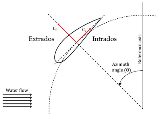
Figure 1.
Sketch of the geometrical configuration of the flow around the turbine. Extrados (outer) and intrados (inner) blade surfaces are also identified.
- Power coefficient:where is the power generated by the turbine and is the frontal area of the turbine. It must be noted that the value of is modified in the turbine configuration including winglets by accordingly increasing the blade height; this allows for a fair comparison with the coefficients obtained for the straight blade.
- Torque coefficient:where is the torque produced by the turbine.
- Tangential and normal force coefficients:where is the component of the hydrodynamic force over the blade that is parallel to the chord of the blade profile and is the component that is perpendicular to the chord of the blade profile as shown in Figure 1. This figure also identifies the location of the outer (extrados) and inner (intrados) blade surfaces.
- Tip speed ratio (TSR):Also, it is possible to obtain the pressure, Equation (6), and skin friction, Equation (7), coefficients as the non-dimensional numbers associated with the pressure and wall shear stress magnitude [24].
- Pressure and skin friction coefficients:where is the reference pressure.
2.2. Geometric Model
In this work, all the geometrical features of the model were obtained from [7], which include the turbine configuration and the dimensions of the water tunnel where the turbine was placed. This geometric model was chosen as the Base case in the simulations due to its numerical and experimental characterization in [7]; this allowed for a comparison of turbine performance with and without winglets. In the following, this Base case will be also denoted as straight blade, SB or no winglets configuration. The relevant geometrical turbine parameters are presented in Table 1.

Table 1.
Geometrical parameters of the turbine.
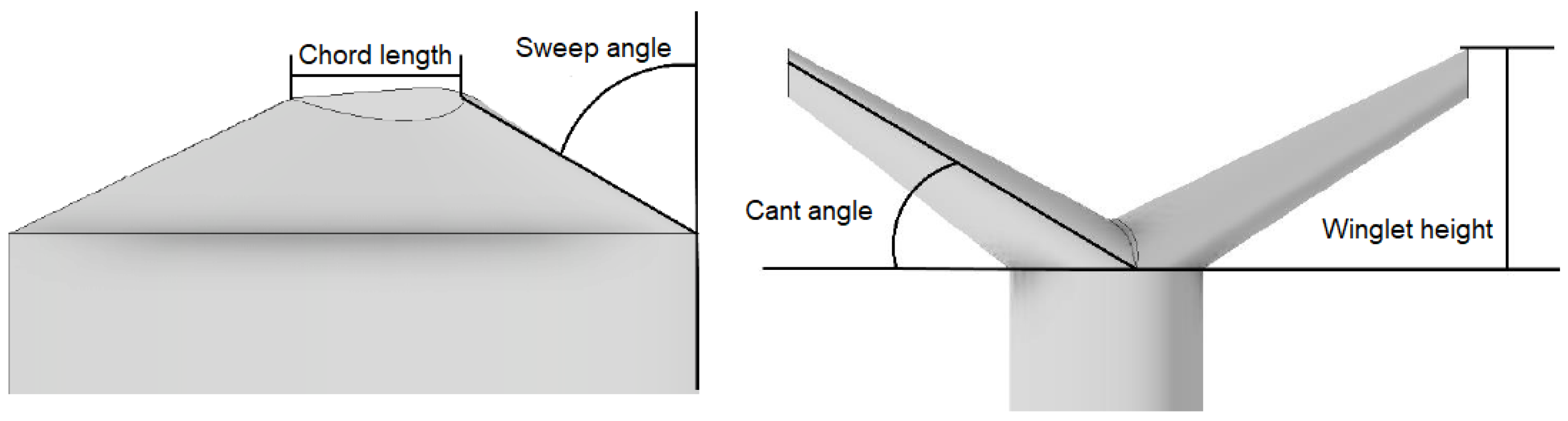
Moreover, since the purpose of this study is to investigate the turbine performance when winglets are used as a flow control device and to find which winglet model among a known range achieves the best performance on the turbine, five winglet models were tested using the symmetric winglet model from [22] as a basis. Four parameters were used to control the shape of winglets: cant angle, sweep angle, winglet height and length of the profile’s chord at the winglet tip. These parameters are presented in Figure 2. However, in the present study, only two of these parameters were used to control the winglet shape, sweep angle and cant angle.
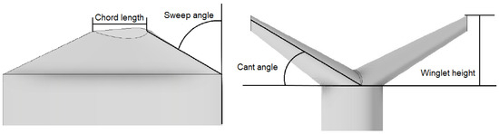
Figure 2.
Illustration of winglets design parameters.
First, the effect of cant angle on the average power extracted by the turbine is assessed by fixing the sweep angle as 60°. Three levels are considered for the cant angle, all with the same winglet height: 15°, 30° and 45°. From them, the angle providing the highest average value is selected. Second, with the chosen cant angle, two additional levels of sweep angle are evaluated: 45° and 75°. From these three combinations, that with the best performance (largest power coefficient) is designated as the best. Table 2 collects the employed values for the parameters in each winglet model.
Table 2.
Reference values for the parameters of each winglet model.
As just described, in Table 2, models 4 and 5 depend on the simulations of the previous three models.
3. Mesh and Computational Set-Up
Three-dimensional unsteady simulations of the dynamic behavior of the turbine were carried out using the overset mesh strategy. Therefore, two meshes were needed for the computational domain: one mesh over the turbine, which is the rotating part of the model (rotational domain), and another grid for the water tunnel (steady domain). In addition, overset meshes need an interface between the rotational and steady domains where the solution is interpolated from the information of both domains [25]. The main features of the computational domain used in the simulations are presented in Figure 3 and Figure 4.
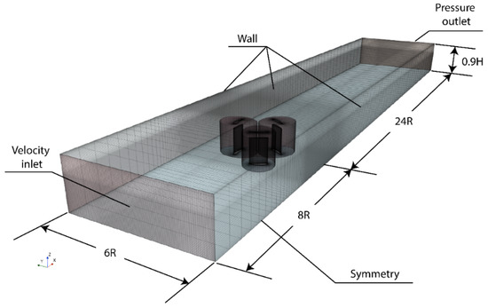
Figure 3.
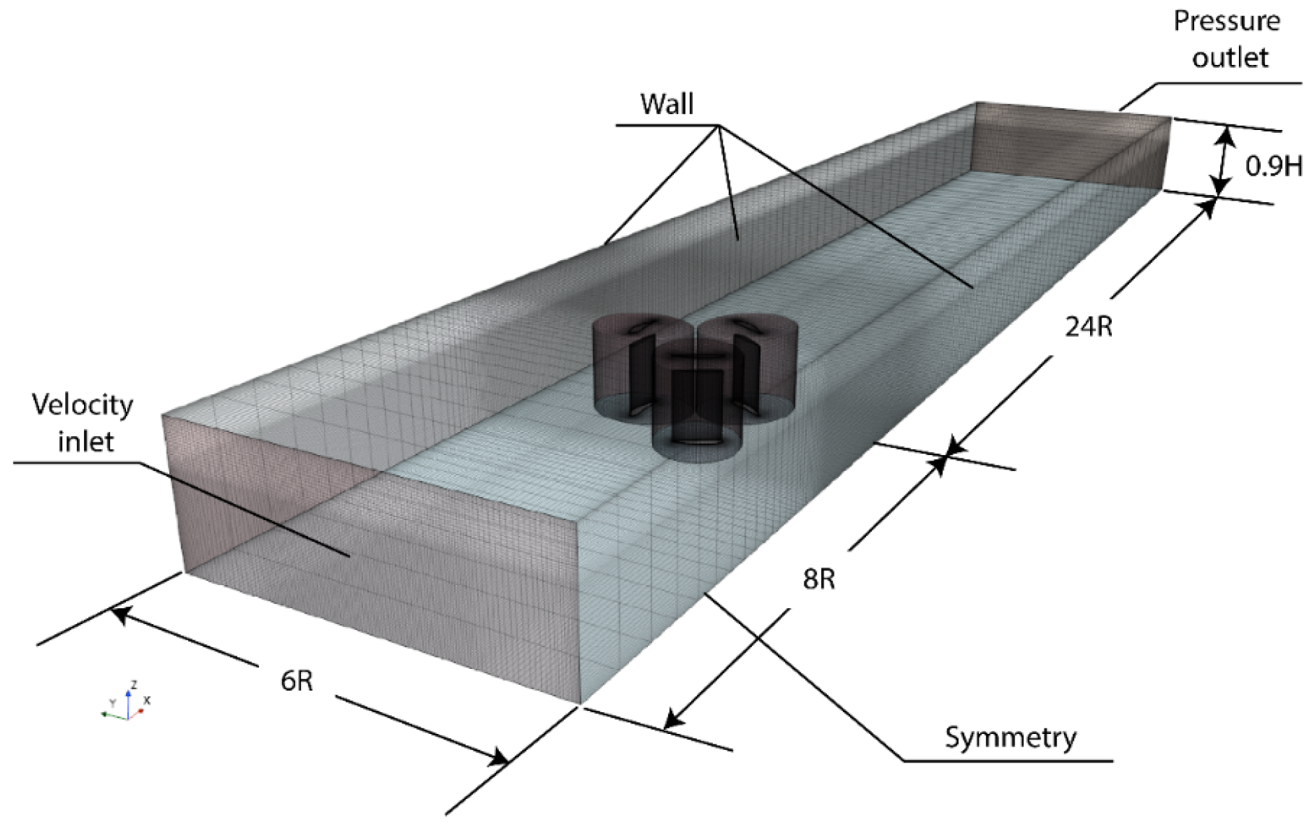
Boundary conditions in the steady domain and its dimensions.
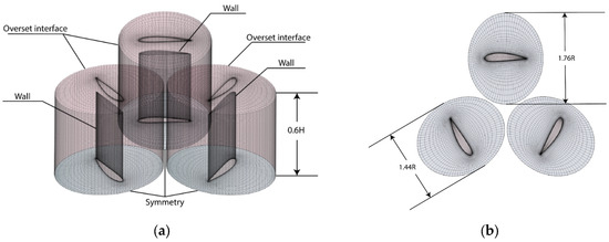
Figure 4.
Boundary conditions in the rotational domain and dimensions. (a) Isometric view, (b) top view.
The dimensions and external boundary conditions of the computational domain are the same as those employed in [7]. Therefore, blockage effects affecting the performance of the turbine in the simulations are the same as in the experimental and computational results obtained by [7]. Moreover, because of the flow configuration’s symmetry, numerical simulations utilized only the upper half of the model to optimize computational resources, resulting in a blade height of . Also, according to [7], neither the turbine axis nor the support arms are included in the simulations. The computational domain is composed of a rectangular stationary domain and three oval cylinders encompassing the blades of dimensions (height major axis minor axis, see Figure 4), constituting the overset mesh. The overset mesh rotates with respect to the turbine axis with prescribed angular velocity in the counter-clockwise direction. The left side of stationary domain is defined as a Velocity Inlet boundary condition with a velocity , while the right side is configured as a zero-gauge Pressure Outlet. The mid-span plane of the computational domain is designated as Symmetry, and the remaining boundaries are set as no-slip Wall. The center of the rotor is located at from the inlet.
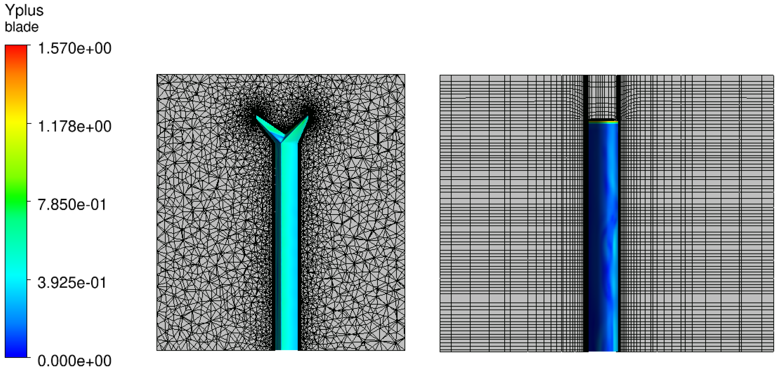
Furthermore, the mesh in the steady domain (the background) is always structured, while in the rotational domain (i.e., the overset region), the mesh is structured in the absence of winglets and unstructured when winglets are present on the turbine (see Figure 5). In both cases, the first cell presents a value well within the viscous region of the boundary layer.

Figure 5.
Mesh details in the overset region in the blade with and without winglets.
For the grid convergence analysis, i.e., the verification study, three meshes were generated decreasing the size of the elements; this information is given in Table 3. The simulations for this study were performed using the configuration of the turbine without winglets or the Base case.
Table 3.
Mesh characteristics.
The simulations were carried out in the commercial software STARCCM+ v2206 considering an incompressible and isothermal flow, assuming water as a Newtonian fluid and neglecting gravitational effects. Moreover, the problem is solved in the transient state, due to the dynamic behavior of the turbine, using URANS (Unsteady Reynolds Averaged Navier Stokes equations) coupled with the SST k-ω Gamma-Re-Theta transition turbulence model [26]. This turbulence model was chosen owing to the Reynolds number calculated on a blade having an approximate value of Re = 30,000, which allows for the transition between the laminar and turbulent flow regime in the turbine. Table 4 presents the setup parameters of the simulation. The employed time step corresponds to of blade rotation according to [7].
Table 4.
Computational parameters employed in the simulations.
Six different cases were studied in the simulations: first, the Base case without winglets and the five different winglet models. For each of these cases, the simulations were performed at . The flow field and integral results were recorded for analysis once the difference between two consecutive cycles was negligible, typically by the twentieth revolution. In addition, after selecting the best winglet model, simulations were conducted at different values to compare the performance curve with the Base case.
Results of Grid Convergence Analysis
A mesh convergence analysis, also called a verification study, was performed to determine the appropriate mesh size to carry out the simulations in the Base case and for . The obtained results are presented in Table 5, showing the average power coefficient along a turbine revolution as a function of the number of cells in each mesh. As it is concluded from that table, the power coefficient tends to stabilize as the number of cells in the mesh increases and the relative difference between the meshes decreases: 2.45% between coarse and fine mesh and 0.6% between fine and extra-fine mesh. Thus, it is observed that for finer meshes, the average power coefficient obtained will not vary with further grid refinement.
Table 5.
Results of the grid convergence analysis.
Moreover, the error between the extra-fine mesh and the numerical analysis at , as conducted by Yagmur et al. [7], is 4.9%, which falls within an acceptable range. Therefore, the extra-fine mesh was selected to carry out the simulations, seeking to minimize the propagation of the error by including the winglets in the simulations.
4. Results and Discussion
4.1. Validation of Simulations versus Reference Study [7]
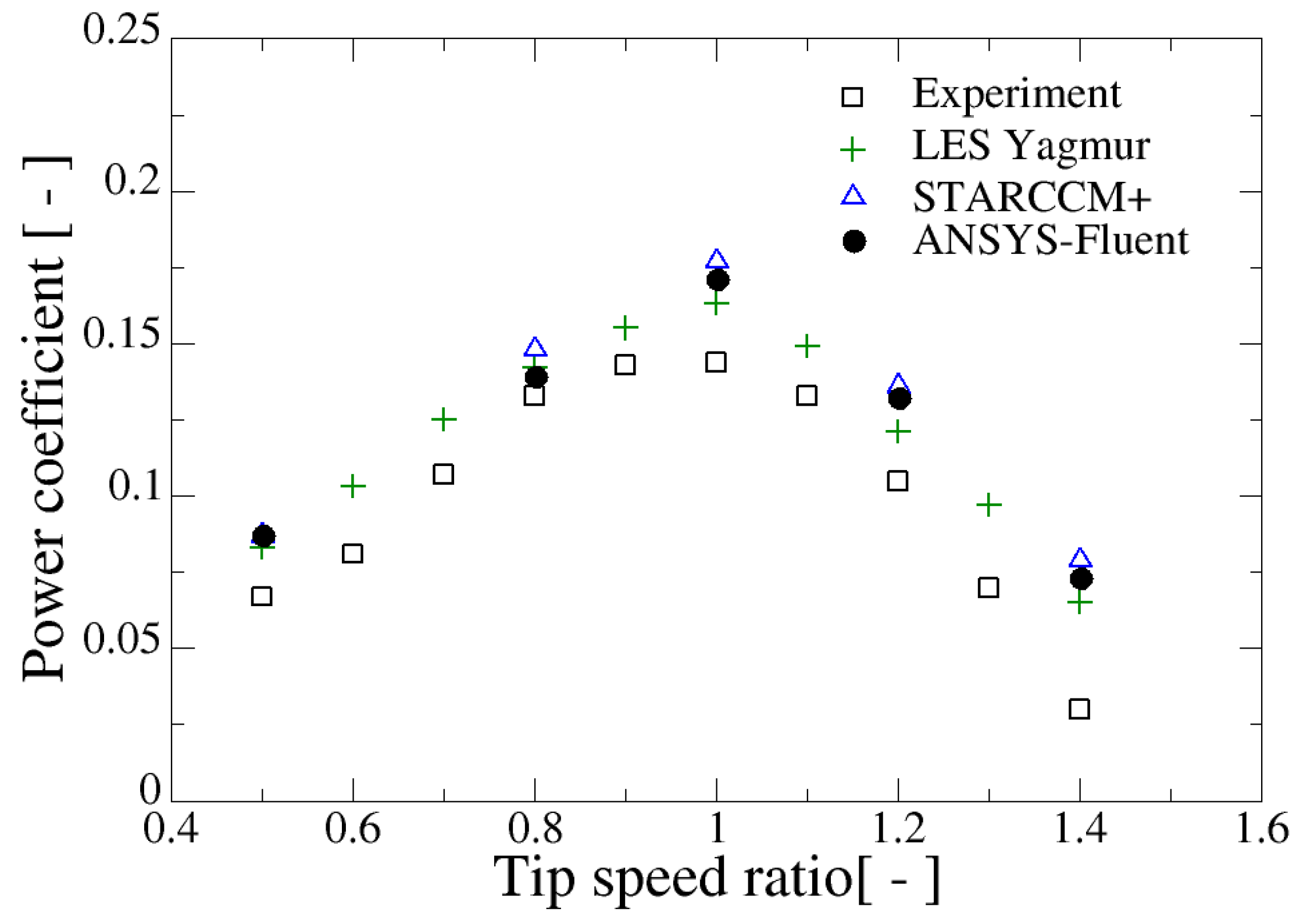
Yagmur et al. [7], provided explicit values for their experimental and numerical average power coefficient at . Those are collected in Table 6 together with that obtained in the present simulations. It is seen that the numerical values of [7], based on Large Eddy Simulation, LES, are above the experimental measurements and that the present results based on URANS are also higher than those of LES; however, the difference between them is lower than 5%, as commented in the previous paragraph.
Table 6.
Comparison of the average power coefficient between [7] and present study.
Moreover, Figure 6 presents the comparison of curves in the Base case (i.e., without winglets) of the present study and the experimental and numerical curves of [7].
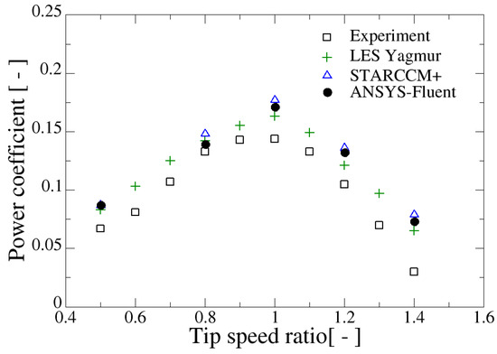
Figure 6.
Total power coefficient curve versus TSR for the hydrokinetic turbine of [7], i.e., in the configuration without winglets.
In order to provide better confidence about the obtained results in the performed simulations of the turbine Base case, in addition to STARCCM+ v. 2206, also the software ANSYS-Fluent v. 2022R1 was employed. In both cases, exactly the same grid (extra fine) was employed in combination with the available SST transition turbulence models in each software. The minor variations in the values of can be attributed to differences in the implementation of turbulence models in each software but typically remain below 5%, thus enhancing the reliability of the obtained results. As can be observed from Figure 6, STARCCM+ tends to provide slightly higher values than Fluent, and both URANS results are above the LES results of [7]. Moreover, all the numerical results are above the experimental measurements, especially for the highest values of TSR, where discrepancies are notorious; the reasons for such overprediction are discussed in [7] but are likely related to some uncertainties in the experimental set up such as “the turbulence characteristics of the tunnel, the centerline position of the turbine, the blade surface roughness and blade-endplate connection screws” [7]; other reasons could be undetectable mechanical and electrical losses in the experimental setup.
Although not shown, the main deviations between the numerical curves for one blade of [7] and the present simulation occurs for azimuthal angles in the downstream cycle, between 300° and 360°. This region is where coherent vortical structures are transported and gathered, significantly influencing the flow development. As a fact, LES provides a better spatial and temporal flow resolution than URANS; consequently, it provides a more accurate description of the evolution of medium-scale vortices, which are typically not adequately resolved using the Reynolds average approach. Therefore, differences between the two numerical approaches are to be expected in the downstroke turbine cycle. As a consequence, the present results for power coefficient slightly overpredict the LES computations.
4.2. Performance of Winglet Models
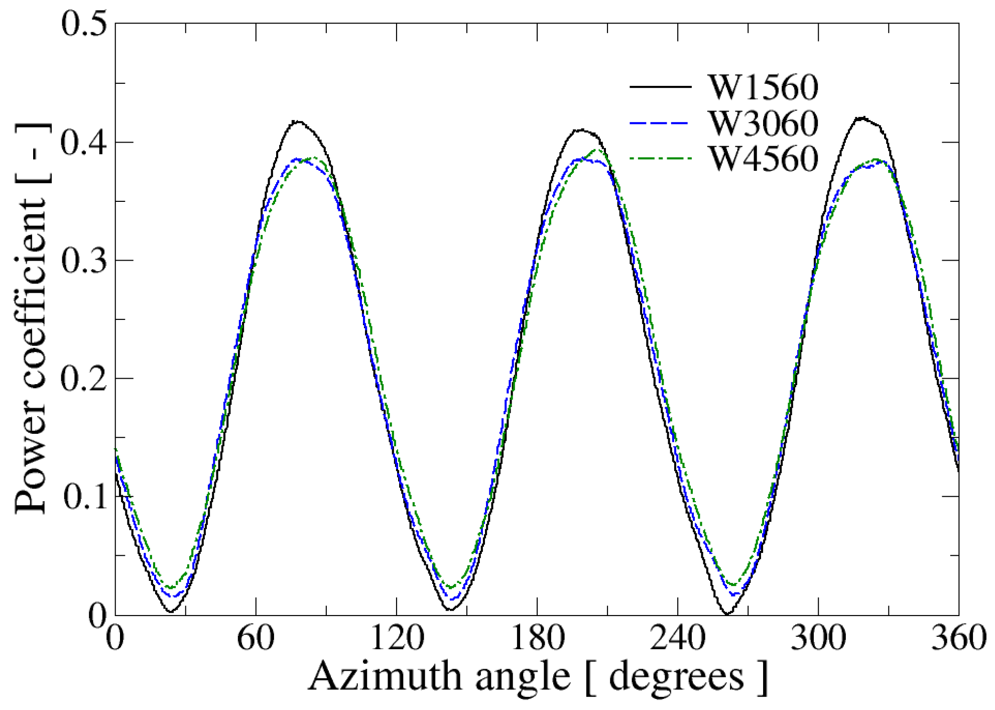
Winglet models were evaluated in two different series of simulations at , i.e., for the optimum operating point. In the first one, models from 1 to 3 were simulated to find out the cant angle that provides the greatest average power coefficient; in the second one, models 4 and 5 were constructed and simulated with the selected cant angle in the first series. From now on, models 1, 2 and 3 of Table 2 are labeled W1560, W3060 and W4560, respectively, explicitly reflecting the cant angle (two first digits) and the sweep angle (two last digits).
Figure 7 shows the instantaneous obtained for the simulation series 1. It is observed that models W3060 and W4560 display very similar behavior, while model W1560 achieves the highest oscillation amplitude in the power coefficient curve. In all cases, the minimum value of is positive, which means that the turbine is able to self-start. When calculating the average power coefficient, = 0.209 is obtained with model W1560, = 0.210 with model W3060 and = 0.214 with model W4560, which yielded the best performance. Model W1560 provides the lowest performance despite having the highest maximum value, which is compensated by its lower minimum values. In fact, the model W4560 is that with the highest minima, presenting very similar maxima to the W3060 model. Actually, the three models exhibit very similar performance with differences between 1.7% and 2.4% with respect to the W4560 model. Likewise, when comparing the W4560 model with the Base case, around a 20% increase in turbine performance is obtained.
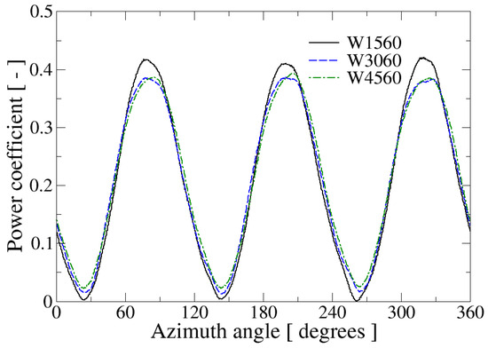
Figure 7.
Comparison of power coefficient between winglet models 1 to 3, varying the cant angle with a fixed value of the sweep angle of 60°.
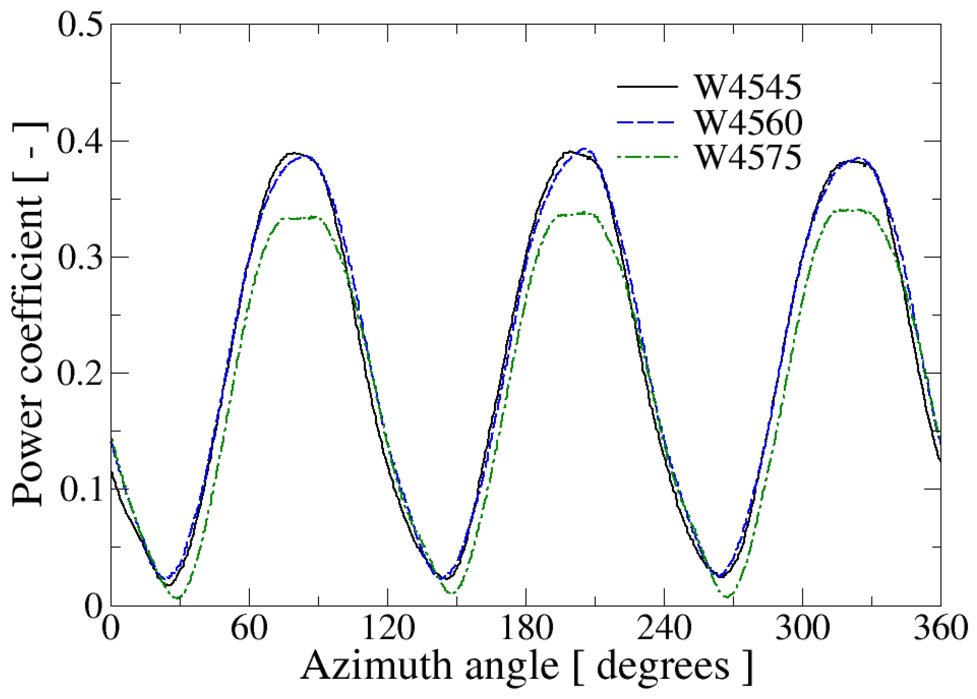
Since model W4560 achieved the best performance on the turbine, it implies that a cant angle of 45° is the best among the angles studied. For that reason, winglet models 4 and 5 were simulated using this angle, labeled W4545 and W4575, respectively. The obtained instantaneous power coefficients for such blades are shown in Figure 8.
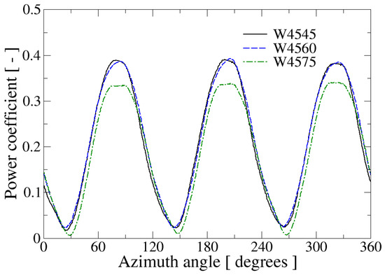
Figure 8.
Comparison of power coefficient between winglet models with 45° cant angle (models 3 to 5 of Table 2).
According to Figure 8, model W4575 shows the smallest amplitude with the bluntest maxima among the three curves, so it is expected to be the one with the worst performance. On the other hand, models W4545 and W4560 have similar behavior. Thus, the average power coefficient is = 0.209 for model W4545 and = 0.189 for model W4575. Therefore, model W4560 remains the model with the best performance among the different models studied. As a remark, it should be noticed that in all cases, the use of winglets improves turbine performance, with increments of 9.5% in the worst case (W4575) and around 20% in the best case (W4560).
From the previous figures, it can be concluded that winglet configurations with cant angles between 30 and 45 degrees combined with sweep angles between 45 and 60 degrees provide quite similar performance results. Among them, the W4560 shows the highest value so this is the selected winglet geometry. In the following, this configuration will be referred to as the winglet blade, WB or W4560 model.
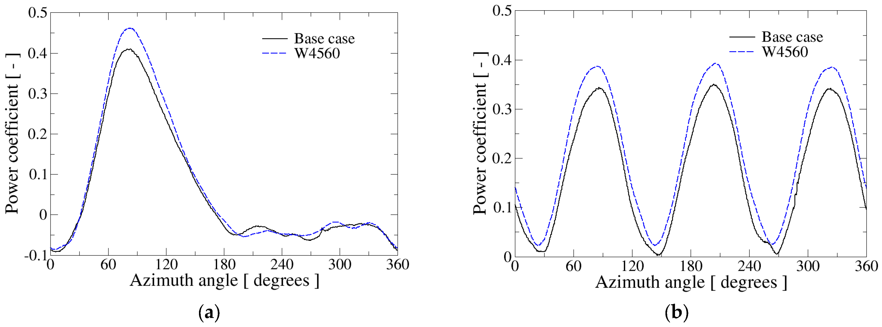
It is instructive to compare the instantaneous curve between the no winglets (Base case) and the W4560 configurations at . The evolution of the power coefficient along a revolution for one blade is presented Figure 9a, while Figure 9b shows the total time-dependent in a cycle.
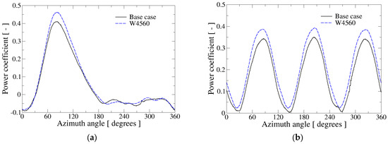
Figure 9.
Evolution of instantaneous power coefficient along a turbine revolution. (a) One blade; (b) three blades.
Figure 9a shows clearly that the main effect of the winglets is produced in the upstream region (azimuthal angle less than 180°), achieving an increase in the power coefficient in the azimuth angle range from 30° to 140°. After the 140° azimuthal angle, in the downstream region, the behavior of the curves is similar with minor differences. As a result, when comparing the total of both cases in Figure 9b, the use of the winglet results in an improvement in the performance of the turbine along the entire turbine cycle, increasing both the minimum power as well as the maximum power produced by the turbine. The fact that the use of winglets augments the minimum torque is beneficial because the turbine self-starting capabilities are improved.
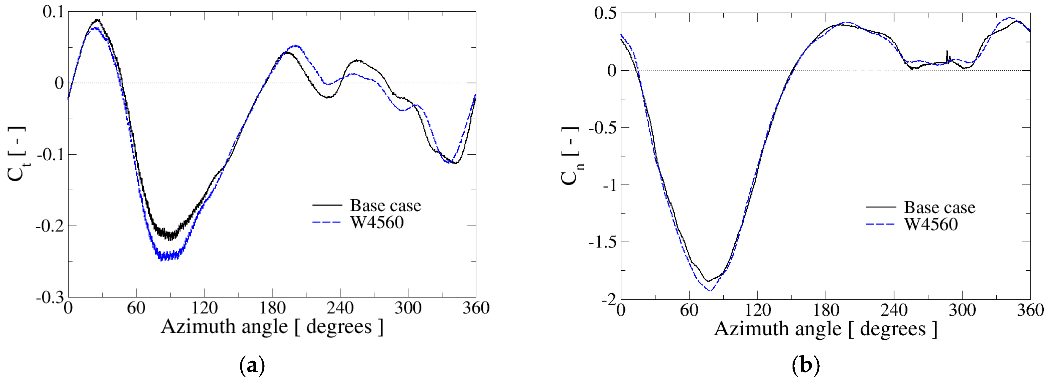
Figure 10 shows the evolution of the tangential (Figure 10a) and normal force (Figure 10b) coefficients acting on one of the turbine blades. The negative tangential force is directly related to the turbine torque and power production, while the negative normal force is related to the cyclic forces acting on the turbine shaft. In both forces, it is observed that the winglet effect produces a general increment in force in the upstream region; in the case of the tangential force, this occurs between 15° and 140° of the azimuthal angle and in the normal force between 20° and 90°. In the downstream region, the curves of the turbine with winglets fluctuate over the behavior of the Base case, showing various crossover points.
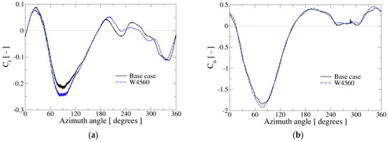
Figure 10.
Evolution of instantaneous force for one blade along a turbine revolution. (a) Tangential force; (b) normal force.
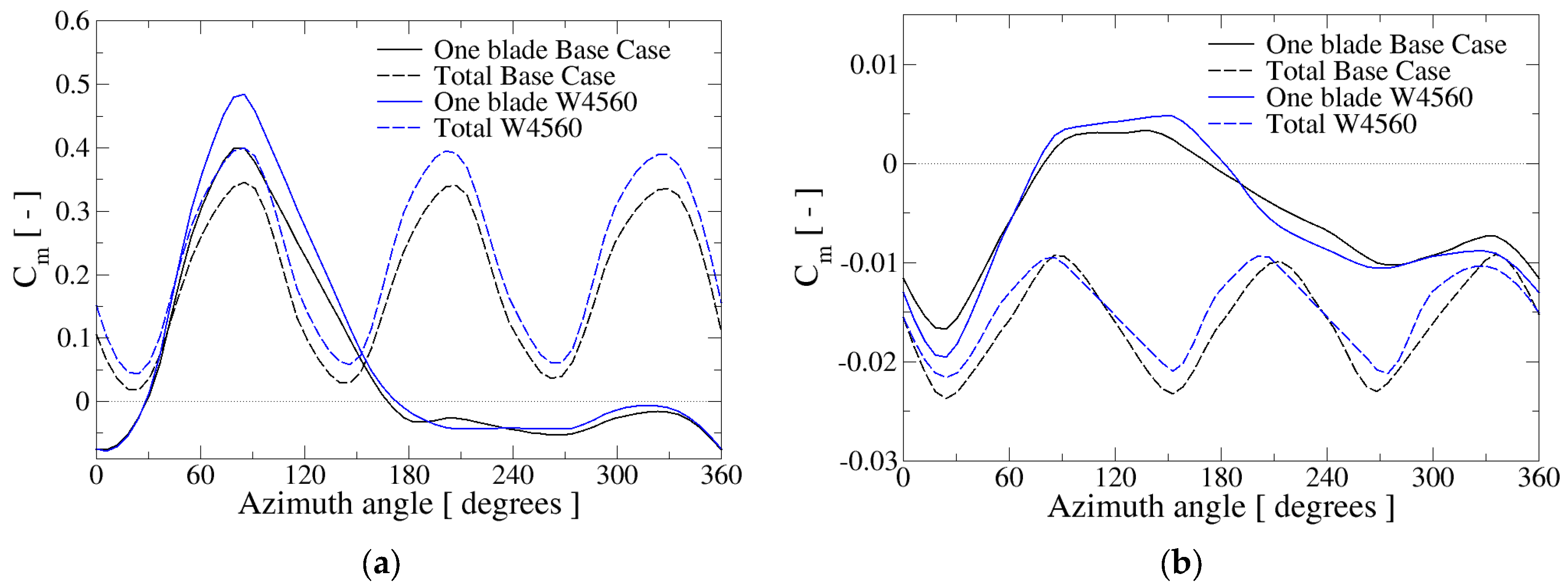
Figure 11 presents the pressure and friction contributions to torque coefficient , Equation (2) in both configurations, with the SB and WB at the design tip speed ratio . From this figure, it is clearly observed that pressure is the dominant contribution to torque coefficient. This was an expected result owing to the high-flow Reynolds number of the order 104. Therefore, the curves for pressure contribution shown in Figure 11a are very close to those in Figure 9, for one blade as well as for total . From Figure 11b, it can be appreciated that the friction contribution to the torque coefficient of one blade is usually negative in both configurations, SB and WB, being slightly positive only in the azimuthal locations between 75 and 180 degrees. Also, the contribution of friction in the winglet blade is larger than in Base case in magnitude. Therefore, when looking at total , it is found that the friction component always tends to reduce the turbine torque which explains why numerical simulations based on potential approaches tend to overpredict turbine performance regarding CFD methods. Also, from Figure 11b, it is noticed that the friction contribution in WB is slightly lower than in SB, due to compensation effects among blades, which is another reason to explain the increase in the performance of winglet blades.
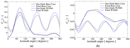
Figure 11.
Pressure (a) and friction (b) contributions to torque coefficient at along a turbine revolution for the two considered configurations, Base case and W4560. One blade and total contributions.
4.3. Characterization of the Turbine and the Best Winglet Model at Different TSR Values
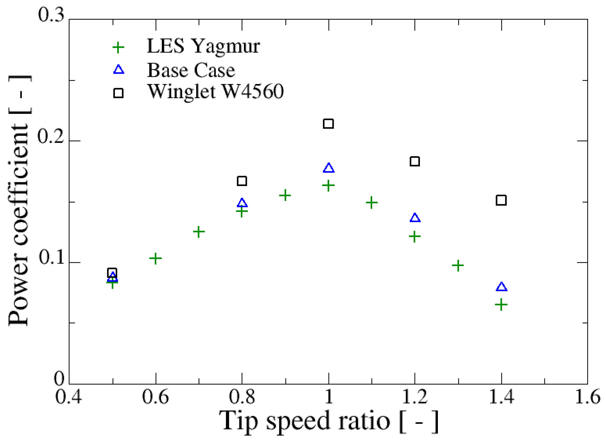
Since the turbine can operate at different rotation speeds or with variable flow velocity, it is necessary to characterize the behavior of the system under different operating conditions. Figure 12 shows the obtained average power coefficient at different TSR values in the numerical study of Yagmur, the Base case and the turbine with the winglet model W4560. From that figure, it is readily noticed that the use of winglets predicts an enhancement of the average in whole range of considered ; however, it is observed that the improvement increases as the tip speed ratio augments ranging from 5% at to nearly 40% at . At , where the curve attains its maximum, the average power coefficient improvement is around 20%, a value similar to that reported in reference [21] for wind turbines and [22] for hydrokinetic turbines.
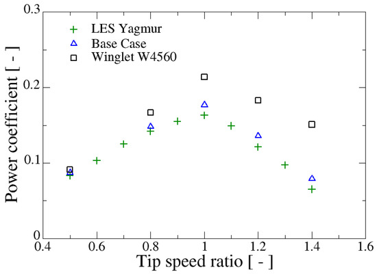
Figure 12.
Variation of power coefficient versus tip speed ratio for the W4560 winglet model compared with the Base case and the LES simulations of [7].
5. Examination of Flow Structures on Straight and Winglet Turbines
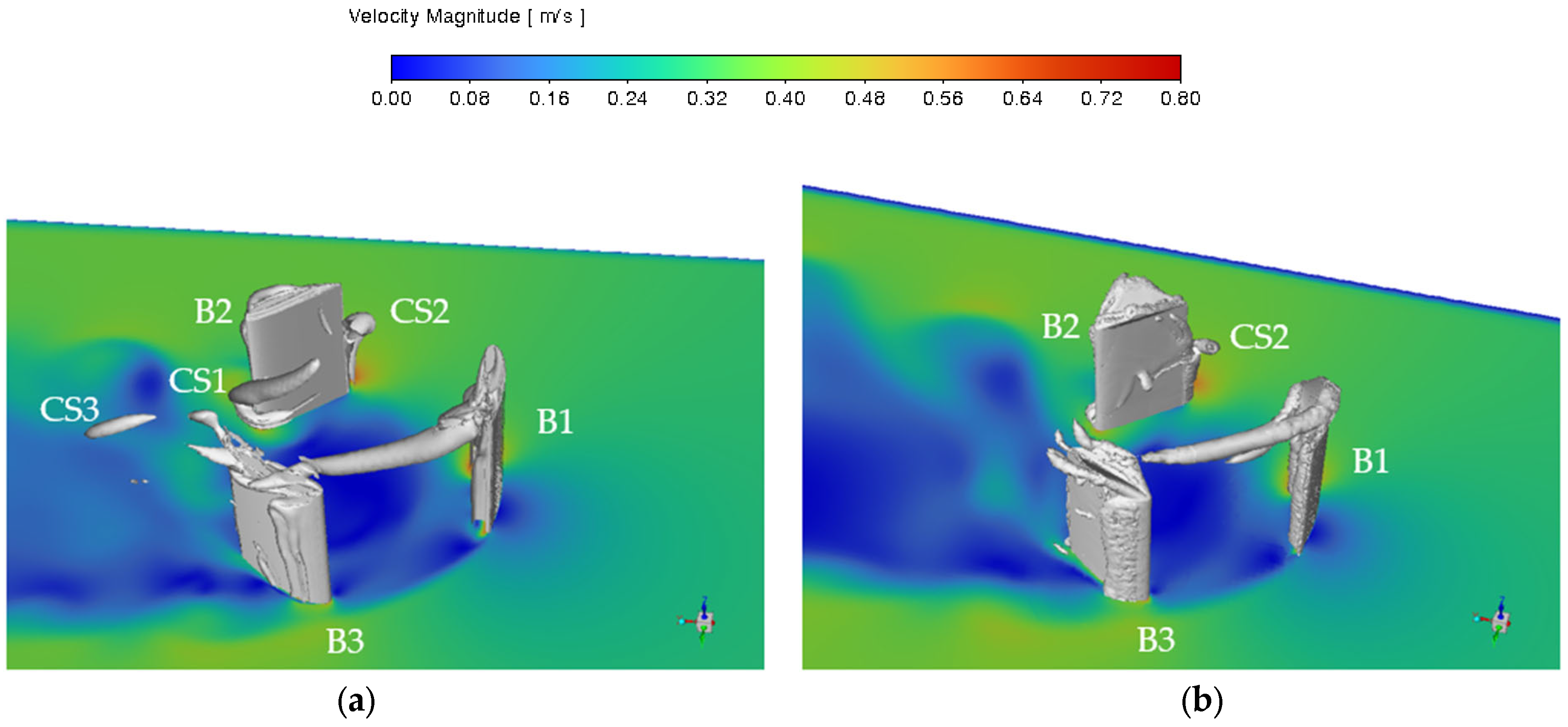
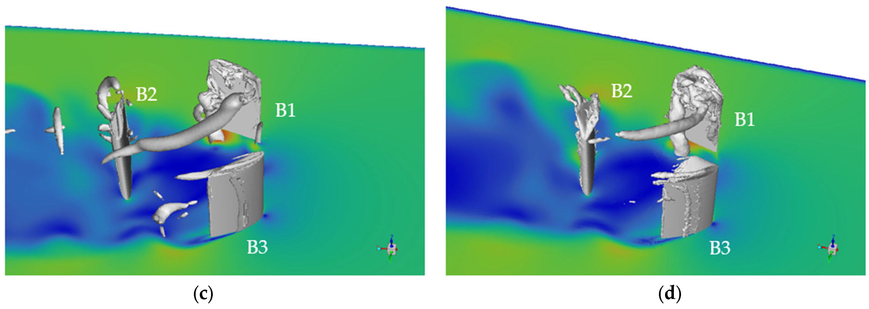
As an illustration of the flow around the turbines, Figure 13 shows the Q-criterion iso-surfaces of 40 s-2 for two angular positions of the first blade, (upper row) and (lower row), in the Base case (left column) and in the W4560 configuration (right column). In such figure, the flow advances from right to left along the positive -direction. Also, the velocity field at the symmetry plane is displayed.

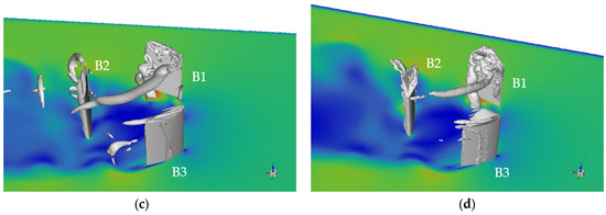
Figure 13.
Iso-surfaces of Q-criterion, Q = 40 s−2, for two azimuthal positions of first blade in the Base case (left column) and winglet (right column) configurations. (a,b) ; (c,d) . Flow progresses along the positive -direction.
In the configuration SB at (Figure 13a), a distinct tip vortex is visible behind blade B1, which is convected downstream by the main flow. Such vortical structure is thick, long-lived and so long that it interacts with blade B3. In fact, the region CS1 represents the remains of the tip vortex detached from the previous blade B2. Around blade B2, a bound vortex CS2 can be distinguished close to the trailing edge while an extra coherent structure CS3 is identified behind blade B3. In the configuration with winglets, Figure 13b, the tip vortex has been split into two components, one at each winglet side. The component emerging from the extrados (outer) side is longer and thicker than its counterpart originating from the intrados (inner) side; however, it is shorter and thinner than the tip vortex in Figure 13a. This observation suggests that the strength of the tip vortices generated by the winglet is lower than in the straight blade, a fact reinforced by the absence of structures similar to CS1 and CS3 in Figure 13b. Moreover, the extrados tip vortex does not reach B3 (as in Figure 13a) and the size of the bound vortex close to the trailing edge of B2 is smaller in the winglet configuration than in the Base case.
At the angular position of (Figure 13c), the tip vortex has been fully detached from B1 in the straight blade, but it is still attached in the winglet configuration (Figure 13d). This fact indicates that another beneficial effect of the winglets is delaying the process of vortex shedding. As noted previously, such vortex is shorter and thinner when it originates from the winglet. Additionally, the number of visible vortical regions in Figure 13d is lower than in Figure 13c, reassuring the observation that the winglet promotes lower-intensity vortices than the straight blade. Looking at the leading edge of B1 in Figure 13c,d, the presence of the so-called –vortex can be noticed. This kind of vortex was identified in a straight blade vertical hydrokinetic turbine in [27] and in wind turbines in [21], and Figure 13d demonstrates that it also appears in presence of winglets. Figure 14 shows a closer view of this kind of vortex in both blade configurations at the angular position , where only half of the blade is displayed.
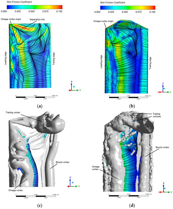
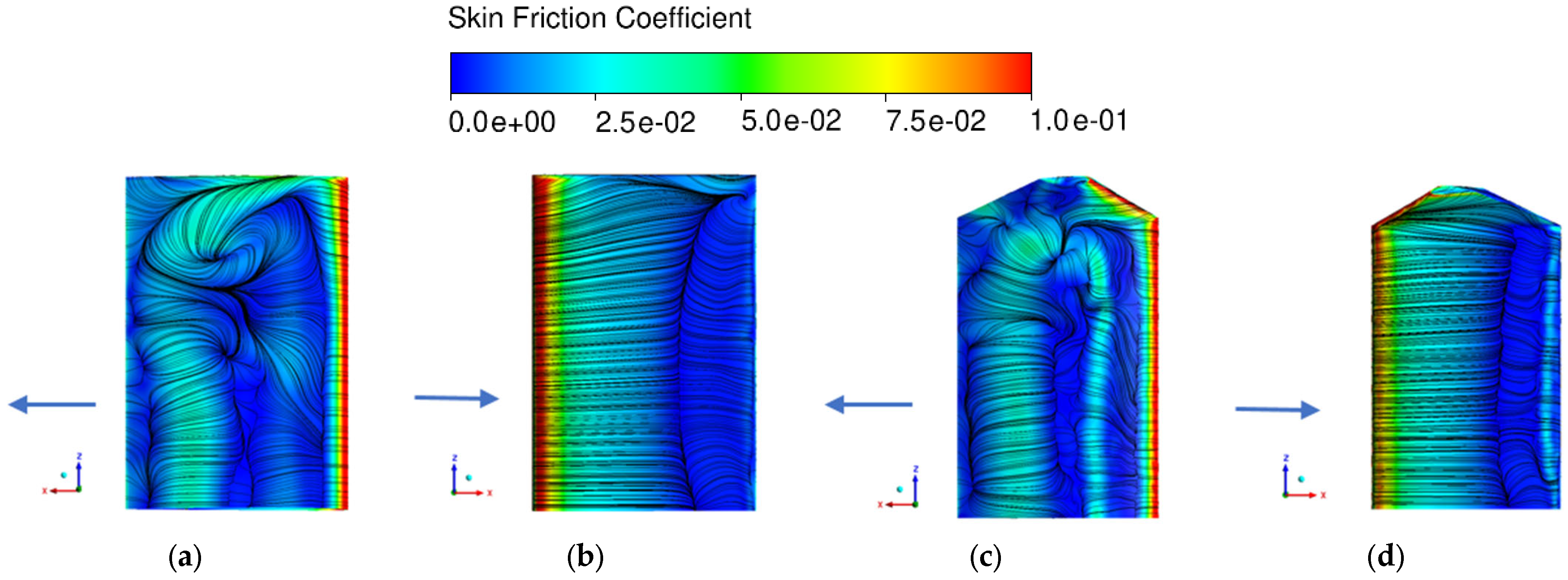
Figure 14.
Illustration of some flow properties around a blade at . Left column: Base case; right column: winglet blade. (a,b) skin friction coefficient with friction lines; (c,d) vorticity iso-surface of 60 Hz.
The omega vortex is typical from the dynamic stall phenomenon on straight wings with flat tips, as discussed in reference [28]. Consequently, the presence of omega vortices in the straight blade during low TSR operation is anticipated. Furthermore, these omega vortices typically combine with the tip vortex to form a vortical system [2,28]. This arrangement is illustrated in Figure 14a,c where a dividing friction line is clearly visible in the upper left zone of the blade (indicated in the plot) separating the two vortices (evidenced by plotting the 60 Hz iso-surface): the –vortex below it and the trailing tip vortex above it (see Figure 14c).
On the other hand, Figure 14 depicts some flow features in the Base case (left column) and in the winglet configuration (right column) at an azimuthal angle of . The upper row of Figure 14 displays the skin friction coefficient , Equation (7), as a contour plot as well as the friction lines. shows higher values close to regions of separation lines where the flow is detached as it can be observed near the leading edge. While the pattern of friction lines is qualitatively similar in both configurations, SB and WB, up to around two-thirds of the blade span, differences arise in the upper third; this fact was also noticed in [21]. In the SB, sharp tip borders become separation lines which promote the formation and detachment of strong tip trailing vortices, while in the WB, the winglet smoothly conducts the flow from its rounded leading edge to the trailing edge with the effect of weakening the strength of the detached trailing vortices (compare Figure 14a and Figure 14b). In the lower row of Figure 14, the 60 Hz vorticity iso-surfaces around both blade configurations are represented. The –vortex is indicated in both cases as well as additional vortical structures, including the bound vortices attached to the trailing edge; in the case of SB, such a bound vortex separates in the upper blade sections, whereas in the WB, it extends along the entire blade span (compare Figure 14c and Figure 14d). The tip trailing vortices are also identified in those figures which consist of one thick component in the Base case but in two components in the W5460, developing from both winglets’ sides; both counterparts are merged as the vortices progress downstream (see Figure 14d).
Figure 15 presents an illustration of the vorticity field in the two considered turbine geometries at two blade sections: mid-span, m (Figure 15a), and the tip plane of the SB blade, m (Figure 15b). The left column corresponds to the Base case and the right column to the W4560 configuration. In the figure, each blade is identified to ease the analysis: B1 is located at , B2 at and B3 at .
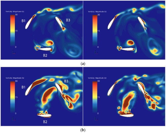
Figure 15.
Vorticity field at B1 azimuthal location of . Left column: Base case; right column: winglet blade. (a) Mid-span plane; (b) turbine tip plane.
At the turbine middle plane, the identified vortical structures are very similar in both turbine designs (Figure 15a). Nevertheless, the following comments can be made in the case WB regarding the SB: the chain of vortices shedding from B1 is more diffuse, the vortex around the extrados of B3 has nearly disappeared and the magnitude of the vortex above the intrados of B2, which is the footprint of the –vortex, is slightly larger.
At the tip plane (Figure 15b), the differences in the vorticity fields around the two blade geometries are more evident. Firstly, the size of the vortical region extending from blade intrados of B1 has been very much reduced in the WB configuration. Second, the large vortex which has detached from B2 intrados reaches B3 in the SB case, but it is much nearer to B2 in the W4560 geometry; this fact demonstrates that the winglet delays the trailing tip vortex separation, reducing the interference of such vortex with B3. Third, for B3, despite that the size and strength of the vorticity field close to the blade seem similar, it is clear that in the case with winglets, the boundary layer is fully attached especially in the extrados; all these effects result in an increase in of that turbine when blades traverse the upstream region.
Analysis of the Behavior of Pressure and Skin Friction Coefficients
In this subsection, the main features of the pressure and friction coefficients on both blade geometries along a turbine revolution are evaluated and discussed. With a few exceptions, these coefficients are usually not examined in the literature dealing with hydrokinetic turbines.
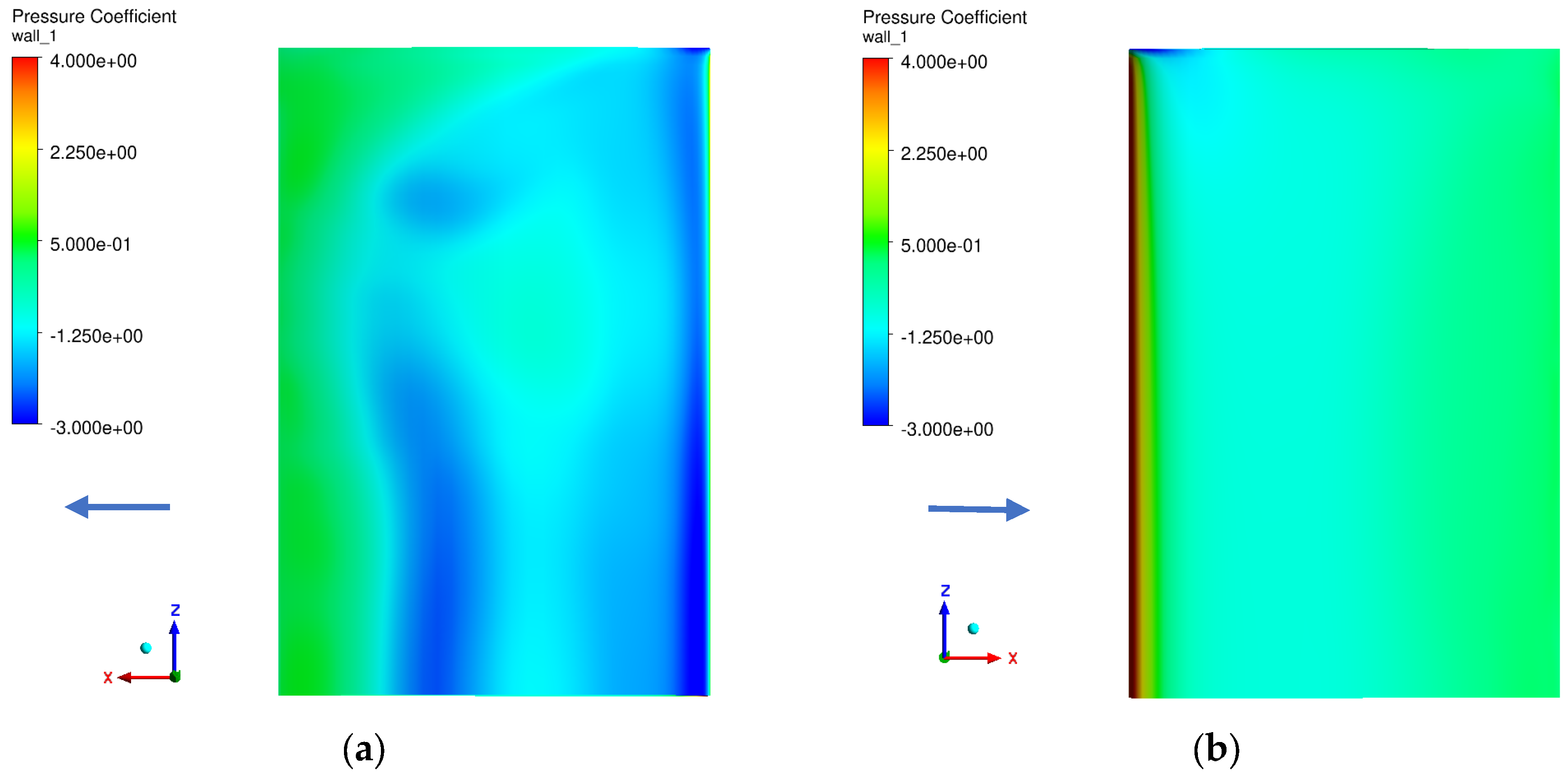
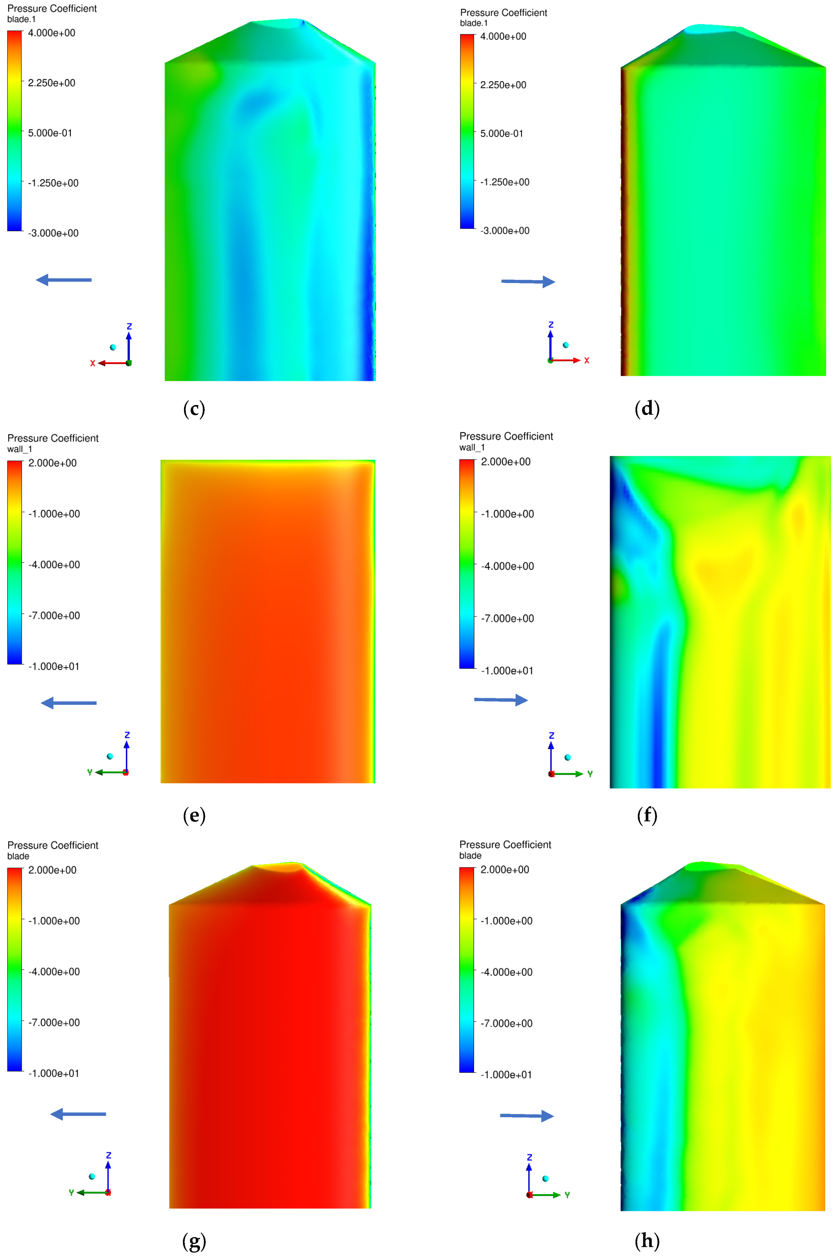
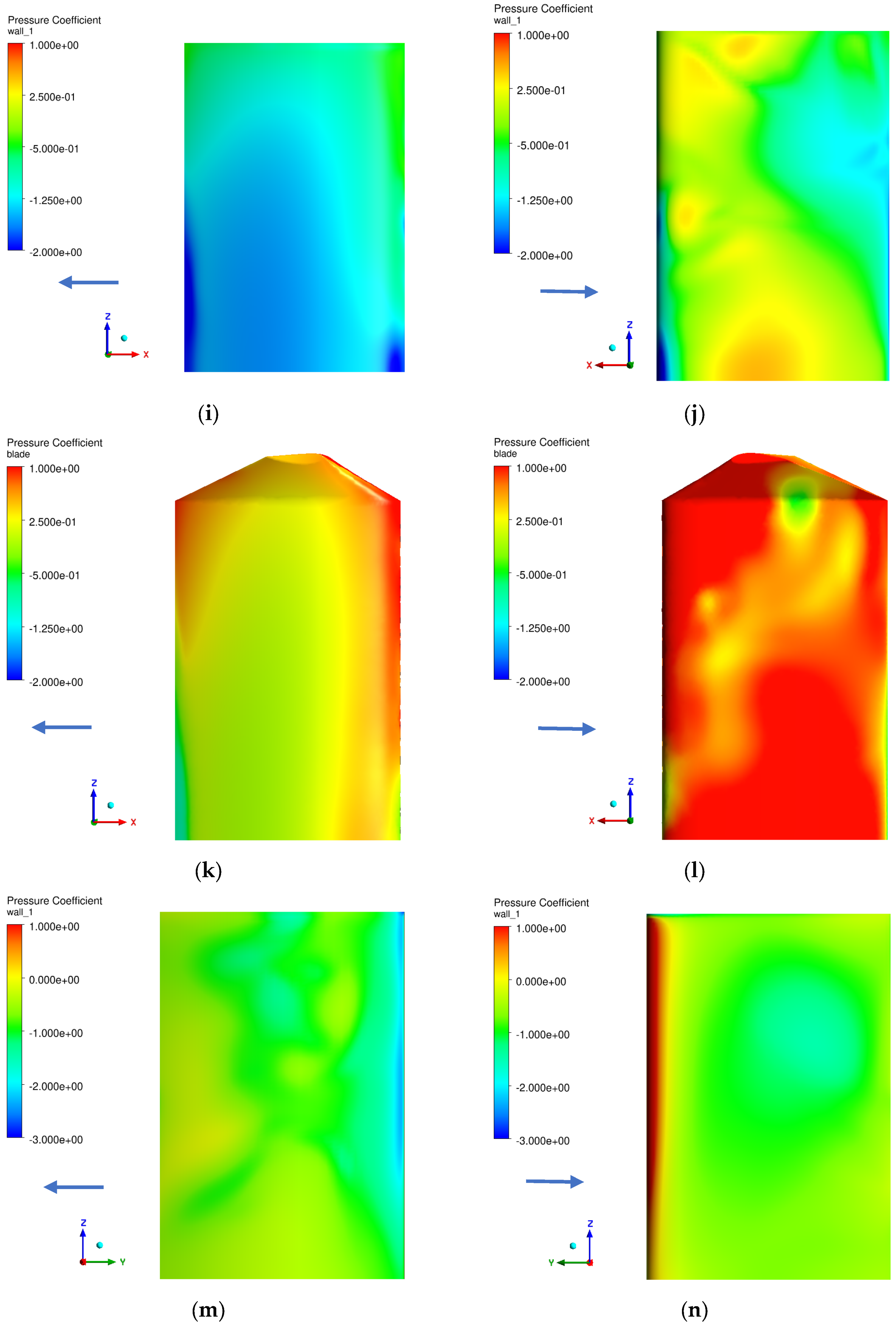
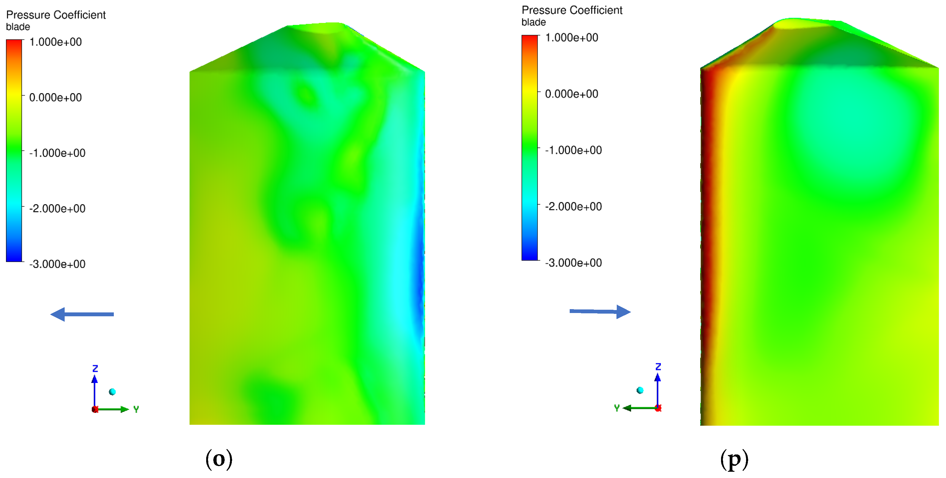
Figure 16 presents the contour plots of the pressure coefficient, Equation (6), for the straight (two leftmost columns) and the winglet (two rightmost columns) blades at and azimuthal angles . Both sides of the blades, the extrados and intrados as shown in Figure 1, are shown; this denomination is preferred instead of pressure and suction sides as the locations of maximum and minimum pressure change along the turbine rotation. The arrow in each subplot indicates the flow direction. Moreover, Figure 17 shows values versus the profile normalized chord (0 meaning leading edge and 1 trailing edge), for the previous azimuthal positions, at two profiles along the blade span: the symmetry plane, m, and very close to the end of the straight blade, m. In the figure, the left column corresponds to the Base case and the right column to the W4560 configuration. In the following, the results are discussed with reference to Figure 16 and Figure 17 simultaneously.
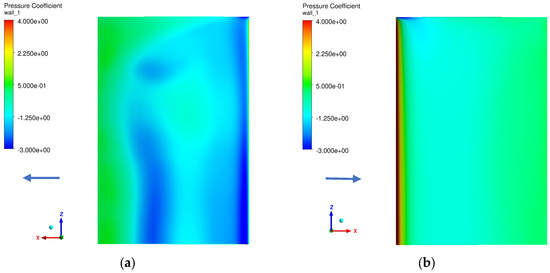
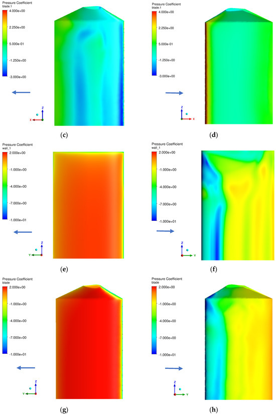


Figure 16.
Contour plots of pressure coefficient at for the straight blade and winglet blade at four azimuthal locations . Arrows indicate the flow direction. (a) , extrados no winglets; (b) , intrados no winglets; (c) , extrados winglets; (d) , intrados winglets; (e) , extrados no winglets; (f) , intrados no winglets; (g) , extrados winglets; (h) , intrados winglets; (i) , extrados no winglets; (j) , intrados no winglets; (k) , extrados winglets; (l) , intrados winglets; (m) , extrados no winglets; (n) , intrados no winglets; (o) , extrados winglets; (p) , intrados winglets.
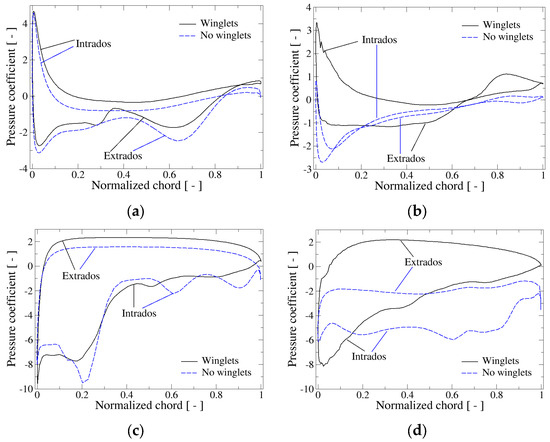
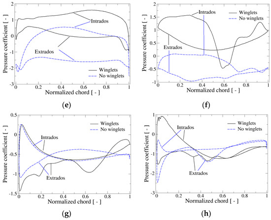
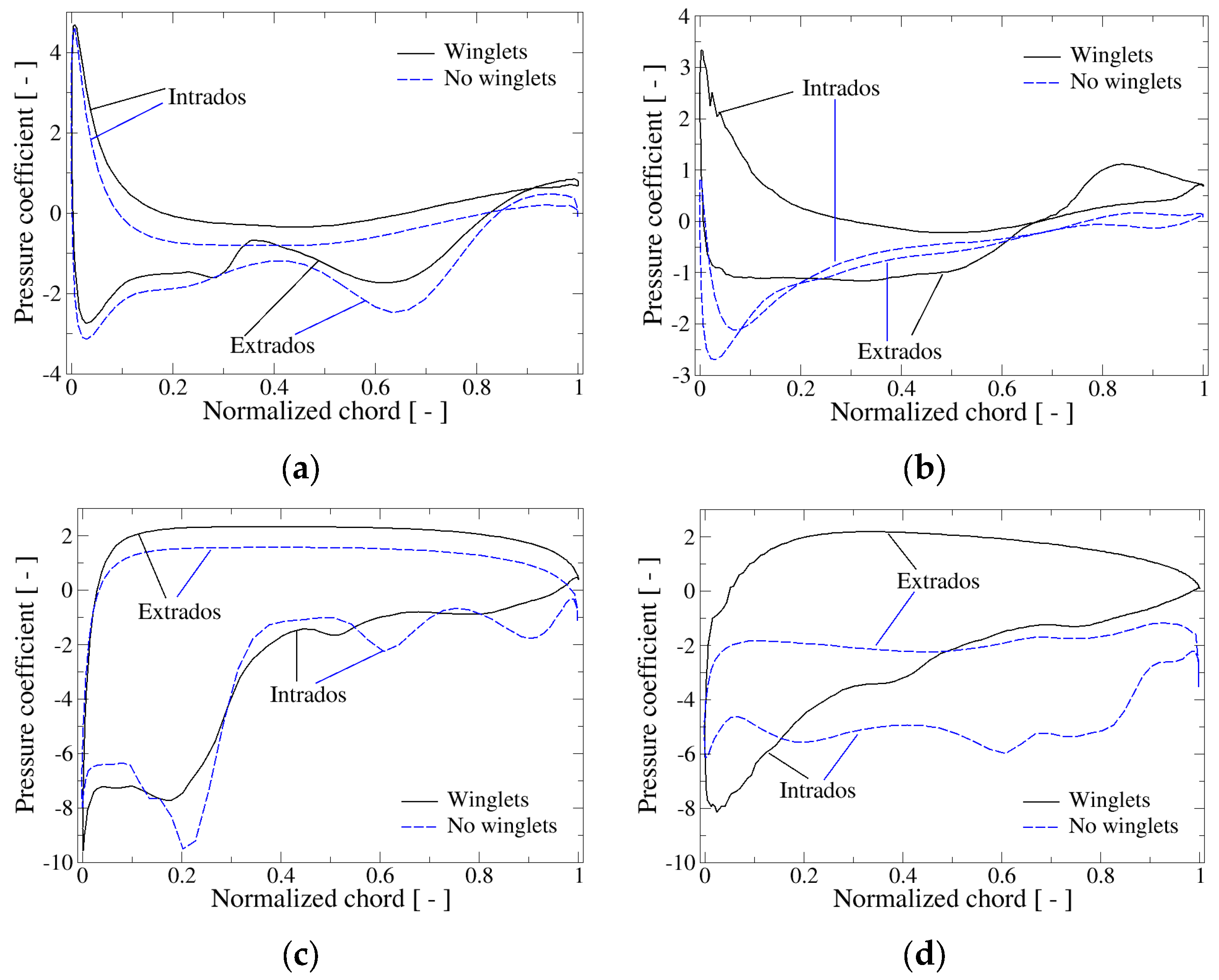
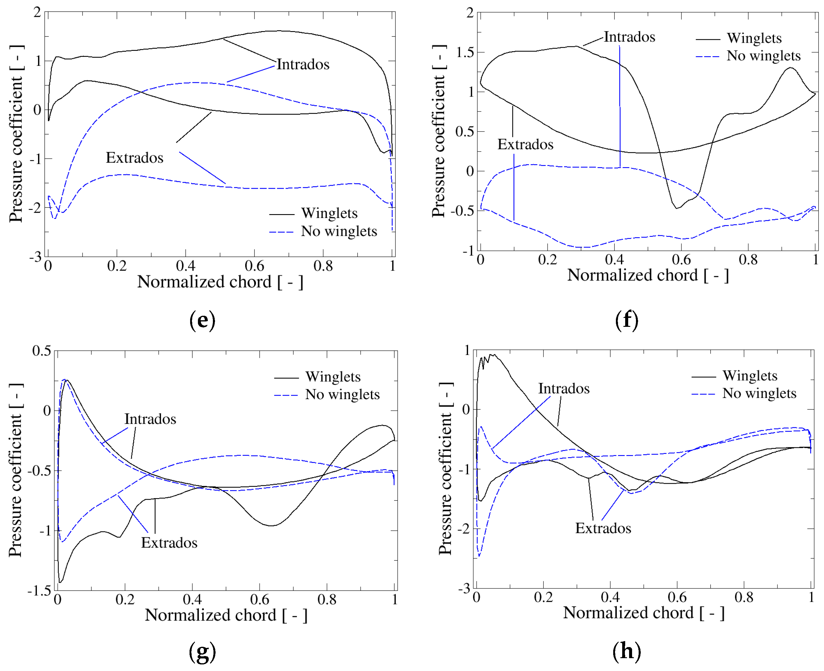
Figure 17.
Profiles of pressure coefficient at for both blade geometries at two sections m (left column), m (right column) and at four azimuthal locations . (a) ; (b) ; (c) ; (d) ; (e) ; (f) ; (g) ; (h) .
At , where the main flow is aligned with the profile chord, the extrados corresponds to the suction side and intrados to pressure side. In the extrados surface, the stream-wise lower value areas of at around two-thirds of the chord are the footprint of detached vortices close to the blade (Figure 16a,c). The intrados of the SB blade shows mainly negative values of the pressure coefficient, differently from the WB blade where it is positive. At the symmetry plane, the profile is very similar in the SB and WB cases with nearly identical maximum and minimum values of the coefficients (Figure 17a); however, the curves for the WB are slightly displaced upwards. At m, a clear change is observed in the Base case where the pressure coefficient in both blade sides is very similar and mainly negative, whereas the W4560 case presents the typical overpressure in the extrados and suction in the intrados.
At the azimuthal location , the second row of Figure 16, the shape of the contours changes substantially regarding , although still the extrados shows positive and the intrados shows negative values of pressure. In this position, the blade is orthogonal to the main flow and, therefore, the extrados side experiences a very uniform maximum pressure (Figure 16e,g). Close to the leading edge of the intrados, strong negative pressure coefficients are seen (Figure 16f,h), which are visible in the curves of Figure 17c,d. The appearance of color fringes on this side reflect the presence of span-wise separated vortices close to the surface. Similar to what happened at at m, the curves for the SB and WB cases are qualitatively very similar, with a gentle upward shift of the latter regarding the former (Figure 17c). However, near the blade tip (Figure 17d), the extrados pressure coefficient in the straight blade experiences a fast decrease and attains negative values (see Figure 16e); as a result, pressures tend to equalize in both surfaces. On the contrary, in the winglet case, the extrados still holds positive values of maintaining the pressure difference between the two sides.
The third row in Figure 16 displays the pressure coefficient at . In this scenario, the main flow is aligned with the blade’s linear displacement, albeit reaching it from the trailing edge. At at this location, it is particular that the blade moves with the same velocity as the main flow, so that some of the vortical structures at the blade tip are able to progress from the trailing to the leading edge, contrarily to the usual direction. is barely positive in the intrados of SB (Figure 16j), while it is mainly positive in the extrados of WB (Figure 16k). Pressure coefficient contour plots on the intrados of both blade configurations reveal a complex structure of detached vortical structures with no clear orientation. Regarding the curves, is the angular position where more differences are found between the two types of blades, as at m, there is a remarkable downward shift in the SB curves (Figure 17e); in particular, there are qualitative differences in the intrados portions of . At the blade tip, m, the pressure coefficient is negative in the Base case and essentially positive in the W4560 geometry, as shown in Figure 17f. In that figure, a sudden drop in in the intrados surface of WB is observed, passing from around to , which is reflected in the green spot visible in Figure 16l; this phenomenon is generated by the detachment of a vortex whose footprint is a localized low value of the pressure coefficient, as mentioned before.
Finally, at (bottom row of Figure 16), the pressure distribution is mainly negative in both blade geometries, except in a short area near the leading edge of the intrados surface. Nevertheless, extrados surfaces exhibit more negative values of . In the upper half of both blades’ intrados, two light blue areas can be noticed (Figure 16n,p), again indicating the presence of a separated trailing vortex close to the surface. Regarding the pressure coefficient curves, at m, they are qualitatively similar for the two geometries (Figure 17g), with those of the intrados being very close while the along the extrados of WB is more wavy than that of SB. At m, the pressure coefficient along both sides tends to equalize in the Base case, being negative, while that in the W4560 configuration reflects pressure differences along the first half of the chord.
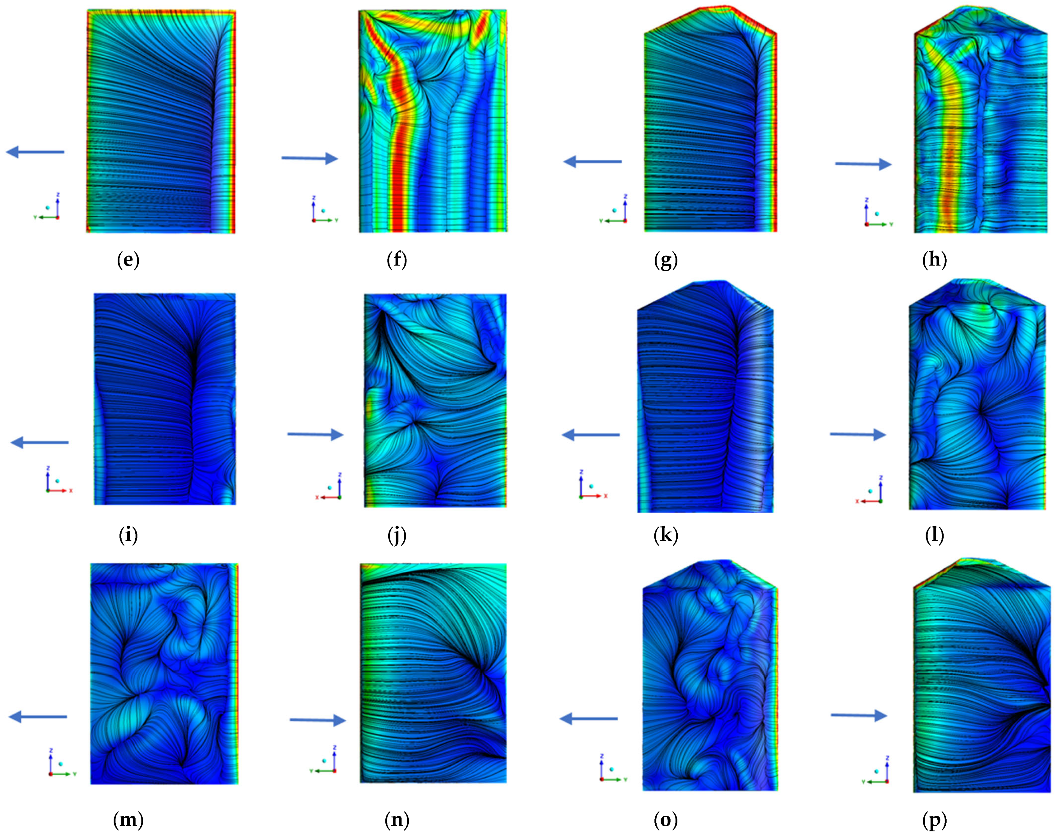
Figure 18 and Figure 19 have the same structure as Figure 16 and Figure 17 but substitute the pressure coefficient with the skin friction coefficient, Equation (7). Moreover, besides the contours of , Figure 18 displays the friction lines on the surface, whose pattern allows for identifying critical flow lines and points [28].

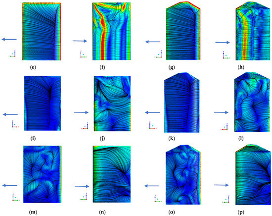
Figure 18.
Contour plots of skin friction coefficient at for the straight blade (two leftmost columns) and winglet blade (two rightmost columns) at four azimuthal locations . In the plots, also the friction line pattern is displayed. Arrows indicate the flow direction. (a) , extrados; (b) , intrados; (c) , extrados; (d) , intrados; (e) , extrados; (f) , intrados; (g) , extrados; (h) , intrados; (i) , extrados; (j) , intrados; (k) , extrados; (l) , intrados; (m) , extrados; (n) , intrados; (o) , extrados; (p) , intrados.
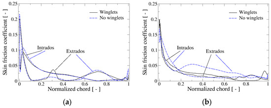
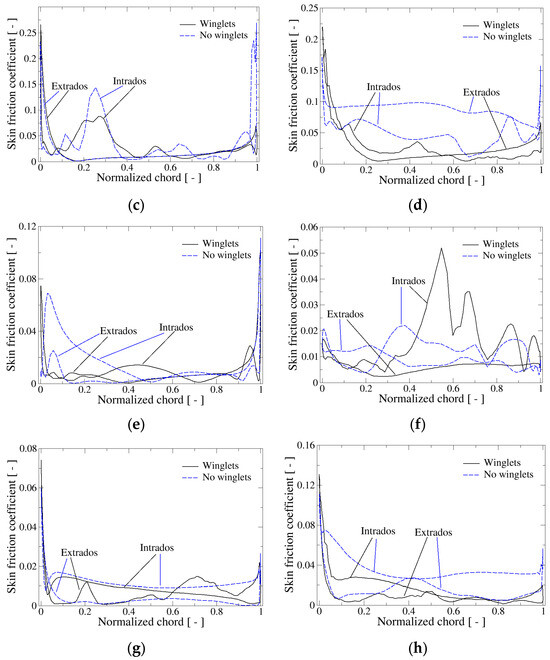
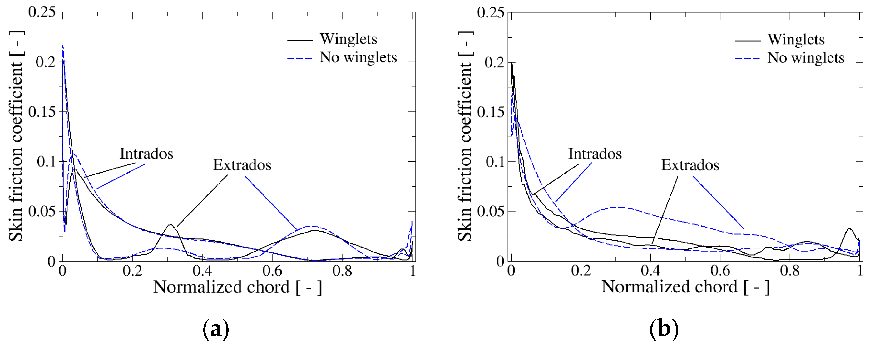
Figure 19.
Profiles of skin friction coefficient at for both blade geometries at two sections, m (left column), m (right column), and at four azimuthal locations . (a) ; (b) ; (c) ; (d) ; (e) ; (f) ; (g) ; (h) .
The first row of Figure 18 shows the behavior of the skin friction coefficient at an azimuthal angle of for the two blade geometries. The intrados surfaces present a relatively simple distribution and friction line pattern (Figure 18b,d): its value is high at the leading edge and diminishes gradually along the profile chord up to the quasi span-wise detachment line where , reflecting separated flow. The contour of skin friction in the extrados is more complex. In the SB geometry (Figure 18a), a separation line, similar to that discussed in Figure 14a, can be observed delimitating the presence of the –vortex and the tip trailing vortex. The footprint of the –vortex close to the surface is the light blue area in the contour plot (showing higher values than the surroundings). A similar situation appears for the WB case (Figure 18c), although in this case the separation line is not so clearly visible; moreover, a thin span-wise light blue strip located at around 30% of the chord is noticed, reflecting the presence of an area of separated flow close to the surface. Regarding the skin friction coefficient curves, at m, they are very similar for the two blades (Figure 19a); in them, various points with can be distinguished, corresponding to separation lines. At m, curves for the intrados and extrados of the winglet blade lie very close to each other, but they differ in the straight blade, where the extrados line is above that of the intrados (Figure 19b).
At , the second row in Figure 18, the roles of the intrados and extrados regarding are inverted; this time, the extrados is that which presents a simpler distribution and friction line pattern, while they are more convoluted in the intrados. In the extrados, for the two blade geometries, the skin friction coefficient is maximum at the leading edge, decreases rapidly up to 0, where a span-wise separation line is observed, and then increases gently up to the trailing edge, where it experiences a faster augmentation. The distribution on intrados surfaces shows span-wise color fringes, revealing the presence of separated span-wise vortical structures. The vertical area colored in red corresponds to an –vortex developing on this surface. Additionally, in the SB case, the footprint of the tip trailing vortex is very clear just behind the leading edge in the upper blade area. Regarding the skin friction coefficient curves, at m, they are qualitatively similar for the two configurations (Figure 19c), although they show some quantitative differences related to the position of the span-wise separated structures. The situation changes at m, where the curves for the Base case are noticeably displaced upwards regarding the W4560 geometry (Figure 19d), reflecting the different dynamics of the flow close to blade tip in both configurations.
The behavior of distribution at is presented in the third row of Figure 18. The extrados keeps the relatively simple friction line pattern in both geometries (Figure 18i,k), developing from the leading edge and showing a separation line in the span-wise direction; in such surfaces, the skin friction coefficient maintains very low values. The intrados side for both blade configurations displays a more convoluted structure of the friction lines with several critical points and lines; also, the contour plot of exhibits spots of higher values of such coefficient, revealing the development of vortical structures close to that surface (Figure 18j,l). The friction line pattern on the intrados is qualitatively similar in the lower half of the blade for the SB and WB configurations, but it differs in the upper half, demonstrating the influence of winglets. In the case of the curves, at m, qualitative differences are appreciated in the intrados although not so much in the extrados: in the Base case, the skin friction coefficient has high values in an area close to the leading edge, but in the W4560 geometry, it diminishes abruptly just behind the leading edge, keeping low values along the profile chord up to reaching the trailing edge where increases suddenly (Figure 19e). At m, the profiles for both sides differ qualitatively and quantitatively; the spotted nature of the skin friction coefficient contour plot in the intrados manifests into peaks and valleys, while in extrados, has higher values in the SB than in the WB configuration (Figure 19f). As a comment, the highest peak present in the intrados of the winglet blade is the wall shear counterpart of the sudden pressure drop observed in Figure 17f, revealing the footprint of a detached vortex close to the surface.
Lastly, the bottom row of Figure 18 shows the contour plot of together with the friction lines on both blade surfaces at . At this location, the involved friction line pattern is present in the extrados in both blade configurations while intrados displays a more regular arrangement. In fact, the wall shear in the intrados decreases smoothly from the leading to the trailing edge (Figure 18n,p). In the extrados, beyond the peak at leading edge, has low values (dark blue) with a few spots of somewhat higher values (light blue) in the proximity of critical lines (Figure 18m,o). Figure 19g presents the evolution along the chord of the skin friction coefficient at the cross-section m; the extrados curve in the winglet blade displays a number of bumps which are not seen in the straight blade (Figure 19g). Moreover, in the former case, the profiles of both surfaces show a cross-over point around 60% of the chord, while in the SB configuration, the wall shear in the intrados is higher than in the extrados along the whole chord length. At m, the curves for the Base case are mainly above those of the W4560 blade (Figure 19h); in particular, in the intrados is larger for the straight than for the winglet blade, due to the presence of the tip trailing vortex close to the surface in the first.
6. Conclusions
This contribution has focused on enhancing the performance of a straight blade hydrokinetic turbine, based on an existing laboratory model reported in [7], by incorporating a symmetrical winglet at its tip. A sensibility analysis study of the winglet design has been carried out by varying the parameters of cant and sweep angles but keeping fixed the winglet height and chord length. As a result, it was determined that the winglet configuration with a cant angle of 45° and a sweep angle of 60° yielded the highest average power coefficient, denoted by W4560. The obtained improvement in performance at the optimal tip speed ratio is around 20%. Furthermore, a comparative analysis was conducted between the straight and W4560 blades, examining the instantaneous power coefficient, tangential and normal forces, as well as the curve. This study also included an evaluation of the pressure and friction components contributing to turbine torque. The final section of the article focuses on examining the vortical flow structures that develop around both straight and winglet blades. This includes analyzing the distribution of pressure and skin friction coefficients at various blade azimuthal positions throughout a turbine revolution.
The main attained conclusions can be summarized as follows:
- While the W4560 design achieved the highest average power coefficient, similar performance enhancements were observed with winglet configurations featuring cant and sweep angles ranging from 30° to 45° and 45° to 60°, respectively, at .
- By analyzing the hydrodynamic coefficients and comparing the base case with the turbine equipped with winglets, it was found that the power generation increase occurs in the upstream region. The rise in such coefficients is generally observed as the turbine moves through azimuthal positions ranging from 30° to 140°.
- The performance improvement with winglets happens over the entire operational range and increases with a growing tip speed ratio.
- One of the main impacts of the winglets is the influence in the tip vortex. The shape, size and strength of the tip vortex are altered due to the presence of the winglets. A second, smaller tip vortex formation was clearly observed due to the symmetrical characteristics of the winglet design.
- Analysis through the flow visualization revealed that the use of winglets weakens the detached trailing vortices and delays the flow separation near the blade tip in the upstream cycle of the turbine. Both effects contribute to the observed increase in turbine power when using winglets.
- In the upper blade area near the tip, the pressure coefficient for the straight blade tends to equalize and become negative on both the pressure and suction sides, whereas in the winglet configuration, the pressure difference is sustained. Additionally, the skin friction coefficient tends to be higher in the SB than in the WB configuration.
One limitation of the current study is that the winglet improvement focused solely on two parameters: cant and sweep angles. In the near future, it is planned to conduct a multi-objective optimization by incorporating additional winglet parameters such as chord length, height, as well as twist and toe angles. Future work will also include experimental work with a turbine prototype with and without the improved winglets in order to verify numerical results presented in this paper.
Author Contributions
Conceptualization, S.L. and O.D.L.; methodology, S.L. and O.D.L.; software, N.B.; validation, N.B. and S.L.; formal analysis, O.D.L. and S.L.; investigation, S.L., N.B. and O.D.L.; resources, O.D.L. and S.L.; data curation, N.B. and S.L.; writing—original draft preparation, N.B.; writing—review and editing, S.L., E.E.N. and O.D.L.; visualization, N.B. and S.L.; supervision, O.D.L. and S.L.; project administration, E.E.N.; funding acquisition, E.E.N. and S.L. All authors have read and agreed to the published version of the manuscript.
Funding
Vicerrectoría de Investigación, Innovación y Emprendimiento of Universidad Autónoma de Occidente through the research project 22INTER-409. This work was also supported by Vicerrectoria de Investigaciones of Universidad de los Andes.
Institutional Review Board Statement
Not applicable.
Informed Consent Statement
Not applicable.
Data Availability Statement
The data presented in this study are available on reasonable request from the corresponding author.
Acknowledgments
Computational resources used were provided by the advanced computer lab and the center for high-performance computing at Universidad de los Andes.
Conflicts of Interest
The authors declare no conflicts of interest.
References
- Kroes, M.J.; Nolan, M.S. Shapes and dimensions of airfoils. In Aircraft Basic Science, 8th ed.; McGraw-Hill Education: New York, NY, USA, 2013. [Google Scholar]
- Tong, G.; Yang, S.; Li, Y.; Feng, F. Effects of blade tip flow on aerodynamic characteristics of straight-bladed vertical axis wind turbines. Energy 2023, 283, 129105. [Google Scholar] [CrossRef]
- Trivedi, C.; Cervantes, M.J.; Gandhi, B.K. Investigation of a high head Francis turbine at runaway operating conditions. Energies 2016, 9, 149. [Google Scholar] [CrossRef]
- Lain, S.; Sommerfeld, M.; Quintero, B. Numerical simulation of secondary flow in pneumatic conveying of solid particles in a horizontal circular pipe. Braz. J. Chem. Eng. 2009, 26, 583–594. [Google Scholar] [CrossRef]
- Marsh, P.; Ranmuthugala, D.; Penesis, I.; Thomas, G. The influence of turbulence model and two and three-dimensional domain selection on the simulated performance characteristics of vertical axis tidal turbines. Renew. Energy 2017, 105, 106–116. [Google Scholar] [CrossRef]
- Lain, S.; Sommerfeld, M. A study of the pneumatic conveying of non-spherical particles in a turbulent horizontal channel flow. Braz. J. Chem. Eng. 2007, 24, 535–546. [Google Scholar] [CrossRef]
- Yagmur, S.; Kose, F.; Dogan, S. A study on performance and flow characteristics of single and double H-type Darrieus turbine for a hydro farm application. Energy Convers. Manag. 2021, 245, 114599. [Google Scholar] [CrossRef]
- Doan, M.N.; Obi, S. Numerical study of the dynamic stall effect on a pair of cross-flow hydrokinetic turbines and associated torque enhancement due to flow blockage. J. Mar. Sci. Eng. 2021, 9, 829. [Google Scholar] [CrossRef]
- Guillaud, N.; Balarac, G.; Goncalvès, E.; Zanette, J. Large Eddy Simulations on Vertical Axis Hydrokinetic Turbines—Power coefficient analysis for various solidities. Renew. Energy 2020, 147, 473–486. [Google Scholar] [CrossRef]
- Singh, E.; Roy, S.; Yam, K.S.; Law, M.C. Numerical analysis of H-Darrieus vertical axis wind turbines with varying aspect ratios for exhaust energy extractions. Energy 2023, 277, 127739. [Google Scholar] [CrossRef]
- Barbarić, M.; Batistić, I.; Guzović, Z. Numerical study of the flow field around hydrokinetic turbines with winglets on the blades. Renew. Energy 2022, 192, 692–704. [Google Scholar] [CrossRef]
- Kunasekaran, M.; Hyung Rhee, S.; Venkatesan, N.; Samad, A. Design optimization of a marine current turbine having winglet on blade. Ocean. Eng. 2021, 239, 109877. [Google Scholar] [CrossRef]
- Wang, Y.; Guo, B.; Jing, F.; Mei, Y. Hydrodynamic performance and flow field characteristics of tidal current energy turbine with and without winglets. J. Mar. Sci. Eng. 2023, 11, 2344. [Google Scholar] [CrossRef]
- Malla, A.; Han, Z.; Zhou, Z. Effect of a winglet on the Power Augmentation of Straight Bladed Darrieus Wind Turbine. IOP Conf. Ser. Earth Environ. Sci. 2020, 505, 012041. [Google Scholar] [CrossRef]
- Miao, W.; Liu, Q.; Xu, Z.; Yue, M.; Li, C.; Zhang, W. A comprehensive analysis of blade tip for vertical axis wind turbine: Aerodynamics and the tip loss effect. Energy Convers. Manag. 2022, 253, 115140. [Google Scholar] [CrossRef]
- Ghiss, M.; Bahri, Y.; Souaissa, K.; Troudi, H.; Ting, D.S.K.; Tourki, Z. Enhancing Vertical Axis Wind Turbine Performance Using Winglets. In Design and Modeling of Mechanical Systems-V. CMSM 2021; Lecture Notes in Mechanical Engineering; Springer: Cham, Switzerland, 2023. [Google Scholar] [CrossRef]
- Mishra, N.; Gupta, A.S.; Dawar, J.; Kumar, A.; Mitra, S. Numerical and Experimental Study on Performance Enhancement of Darrieus Vertical Axis Wind Turbine with Wingtip Device. J. Energy Resour. Technol. 2018, 140, 121201. [Google Scholar] [CrossRef]
- Sham, S.; Khamis, A.; Abdallftah, M.T.; Fares, M.; Shahid, S. CFD Analysis of Vertical Axis Wind Turbine with Winglets. J. Renew. Energy Res. Appl. 2021, 3, 51–59. [Google Scholar] [CrossRef]
- Cai, X.; Zhang, Y.; Ding, W.; Bian, S. The aerodynamic performance of H-type darrieus VAWT rotor with and without winglets: CFD simulations. Energy Sources Part A Recovery Util. Environ. Eff. 2019, 1–12. [Google Scholar] [CrossRef]
- Zhang, T.T.; Elsakka, M.; Huang, W.; Wang, Z.G.; Ingham, D.B.; Ma, L.; Pourkashanian, M. Winglet design for vertical axis wind turbines based on a design of experiment and CFD approach. Energy Convers. Manag. 2019, 195, 712–726. [Google Scholar] [CrossRef]
- Xu, W.; Li, G.; Wang, F.; Li, Y. High-resolution numerical investigation into the effects of winglet on the aerodynamic performance for a three-dimensional vertical axis wind turbine. Energy Convers. Manag. 2020, 205, 112333. [Google Scholar] [CrossRef]
- Laín, S.; Taborda, M.A.; López, O.D. Numerical Study of the Effect of Winglets on the Performance of a Straight Blade Darrieus Water Turbine. Energies 2018, 11, 297. [Google Scholar] [CrossRef]
- Manwell, J.F.; McGowan, J.G.; Rogers, A.L. Wind Energy Explained: Theory, Design and Application, 2nd ed.; Wiley: Chichester, UK, 2009. [Google Scholar]
- Roy, S.; Branger, H.; Luneau, C.; Bourras, D.; Paillard, B. Design of an offshore three-bladed vertical axis wind turbine for wind tunnel experiments. OMAE2017-61512. In Proceedings of the ASME 2017 36th International Conference on Ocean, Offshore and Arctic Engineering OMAE2017, Trondheim, Norway, 25–30 June 2017. [Google Scholar] [CrossRef]
- Steger, J.L.; Dougherty, F.; Benet, J.A. A Chimera Grid Scheme; The American Society of Mechanical Engineers: New York, NY, USA, 1983; Volume 5. [Google Scholar]
- Langtry, R.B.; Menter, F.R. Correlation-based transition modeling for unstructured parallelized computational fluid dynamics codes. AIAA J. 2009, 47, 2894–2906. [Google Scholar] [CrossRef]
- Laín, S.; Cortés, P.; López, O.D. Numerical Simulation of the Flow around a Straight Blade Darrieus Water Turbine. Energies 2020, 13, 1137. [Google Scholar] [CrossRef]
- Spentzos, A.; Barakos, G.; Badcock, K.; Richards, B.; Wernert, P.; Schreck, S.; Raffel, M. Investigation of Three-Dimensional Dynamic Stall Using Computational Fluid Dynamics. AIAA J. 2005, 43, 1023–1033. [Google Scholar] [CrossRef]


Disclaimer/Publisher’s Note: The statements, opinions and data contained in all publications are solely those of the individual author(s) and contributor(s) and not of MDPI and/or the editor(s). MDPI and/or the editor(s) disclaim responsibility for any injury to people or property resulting from any ideas, methods, instructions or products referred to in the content. |
© 2024 by the authors. Licensee MDPI, Basel, Switzerland. This article is an open access article distributed under the terms and conditions of the Creative Commons Attribution (CC BY) license (https://creativecommons.org/licenses/by/4.0/).