Abstract
Addressing the shortcomings of existing ship trajectory compression methods that rely on the empirical setting of a fixed threshold and face challenges in controlling the spatial similarity before and after compression, this paper proposes a self-adaptive compression method for ship trajectories that does not require threshold setting. Initially, a hierarchical and sequential tree structure based on the trajectory characteristics is constructed to determine the importance of a ship’s trajectory points. Subsequently, the dynamic time warping (DTW) operator is introduced to assess the spatial similarity of the trajectory before and after compression, exploring the laws governing similarity variations in the step changes during the compression process from lower to higher levels of the hierarchical and sequential sequence. Finally, the trajectory point that causes the largest step change in similarity within the hierarchical and sequential sequence is identified, and points at lower levels than this point are discarded, thus achieving the objective of self-adaptive adjustment of the level of compression. Our case study results demonstrate that, compared with existing ship trajectory compression methods based on empirically set thresholds, the proposed method has the following advantages: (1) it does not require presetting a fixed threshold and adaptively determines the degree of compression by identifying the trajectory point that leads to the largest step change in similarity, and (2) under the condition of a similar data compression rate, the DTW calculation value is reduced by approximately 25%, significantly enhancing the similarity of the trajectory before and after compression.
1. Introduction
The automatic identification system (AIS) is a pivotal tool for ship identification and maritime traffic management, bolstering safety and regulatory efficiency through the exchange of positional and navigational data. As a critical source for maritime safety management, traffic coordination, behavioral analysis, and environmental preservation [1], the AIS’s importance cannot be overstated. However, the burgeoning number of vessels, coupled with advancements in communication technology, has led to exponential growth in the AIS’s data volume, particularly in congested maritime regions, where data refresh rates may soar to 2–12 s per vessel movement update [2]. This surge in voluminous and frequent AIS data updates presents formidable challenges in data storage, management, and processing. The imperative to maximize the utility of AIS data necessitates the compression of raw data to eliminate redundancies while preserving the essence of ships’ trajectories, thereby diminishing storage demands and enhancing the efficiency of data transmission and analysis [3].
In recent years, scholars have conducted extensive research on AIS ship trajectory compression and have developed a series of optimization algorithms. Bellman [4], leveraging dynamic programming theory, was the first to propose the Bellman algorithm, which optimizes trajectories by minimizing the number of points within a given error threshold. However, this algorithm is characterized by relatively high computational complexity. Subsequently, Douglas and Peucker introduced the Douglas–Peucker (DP) algorithm [5], which utilizes an error distance threshold as the basis for compression. This algorithm is widely acclaimed for its simplicity and outstanding compression performance. Addressing the needs of online compression scenarios, Keogh et al. [6,7] proposed the sliding window algorithm, which continuously updates trajectories by dynamically selecting and removing points through a sliding window, making it particularly suitable for real-time or streaming data processing. Building upon these foundational studies, the academic community has further developed various trajectory compression algorithms, including the TD-TR (trajectory-driven trajectory reduction) algorithm [8] and the Visvalingam–Whyatt algorithm [9]. Muckell et al. [10] conducted a comprehensive comparative analysis of existing trajectory compression algorithms, validating that the DP algorithm surpasses the TD-TR, STTrace, and Bellman algorithms in terms of both computational efficiency and spatial accuracy.
In the DP algorithm, the crux of the trajectory compression’s quality lies in setting an appropriate threshold. Traditional approaches derive these thresholds from empirical analyses that are specific to vessel types and navigational contexts. For instance, Gao and Shi [11] deduced a heading angle deviation threshold of 9° through iterative testing, segmenting compression levels into high, medium, and low, with respective distance thresholds at 43%, 38%, and 33% of the ship’s length. Similarly, Li et al. [12] employed statistical experiments to ascertain the optimal distance threshold for Douglas–Peucker compression, specifically when it was tuned to AIS data within a particular channel. Zhang et al. [13] proposed a threshold defined as the ship’s length multiplied by 0.8, while Wei, Xie, and Zhang [14] adopted this threshold, adjusting for speed and heading variations via a sliding window approach.
However, these methodologies are not without limitations:
- The reliance on a single threshold to control the overall compression ratio of trajectories does not permit nuanced regulation of spatial congruence at an individual trajectory or localized level. Consequently, this may lead to the inadvertent omission of pivotal navigational points in complex maritime areas or the retention of excessive, non-critical points in more open seas, resulting in data redundancy;
- Existing methods rely on empirical thresholds, derived from historical data tied to specific ship types and navigational circumstances; consequently, their applicability may wane with significant contextual shifts.
Spatial similarity is a measure of the consistency of spatial entities in terms of their location, shape, and other spatial attributes [15]. Wang et al. [16] introduced spatial similarity as a metric, establishing a quadratic function relationship between the map scale and simplification threshold for geographic linear features, thereby achieving scale-based adaptive threshold determination. Although this method is only applicable to the adaptive compression of map features with clearly defined scales, inspired by this approach, this paper employs spatial similarity as a quantitative evaluation metric for the compression of ship data and proposes a threshold-free adaptive ship trajectory compression method. Firstly, a hierarchical tree sequence of the importance of ship trajectory points is constructed based on trajectory features. Then, the spatial similarity of the trajectories before and after compression is evaluated using the dynamic time warping (DTW) operator, exploring the pattern of similarity changes during the compression process along the hierarchical tree from low to high levels. Finally, by identifying the trajectory points with the most significant similarity between their step function changes, the number of points retained post compression is automatically adjusted to achieve adaptive compression.
The main contributions and innovations of this paper are as follows:
- This paper proposes an enhancement of the DP algorithm, overcoming the traditional DP algorithm’s limitations in adjusting the similarity in local spatial regions of trajectories, thereby improving the quality of the compressed data.
- The proposed method achieves adaptive compression of ship trajectories without the need for threshold setting by extracting the trajectory points that cause the greatest step change in spatial similarity. To the best of our knowledge, this is the first time that spatial similarity has been used to evaluate the effectiveness of trajectory compression.
- The proposed method is widely applicable and could effectively compress trajectories for various types of ships, including cargo ships, tankers, and fishing vessels.
2. Methodology
Figure 1 illustrates the structural framework of the proposed method. Based on the basic principles of the DP algorithm (Section 2.1), this paper enhances the DP algorithm by constructing a hierarchical and sequential tree structure for the compression of ships’ trajectory points (Section 2.2). Then, the trajectory points are compressed from the bottom to the top along this hierarchical sequence tree structure, and the step changes in similarity during this process are explored (Section 2.3). Finally, according to the change patterns, the maximum step change points are used for adaptive compression of the trajectories (Section 2.4).
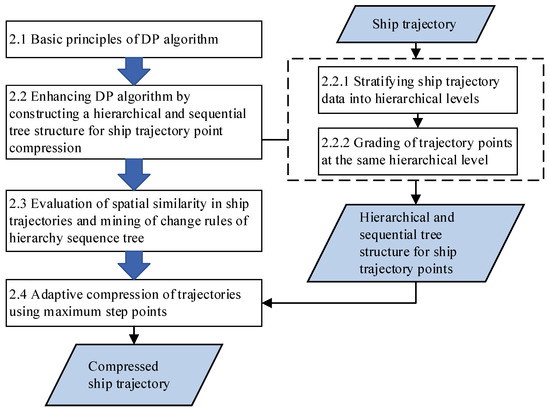
Figure 1.
Structural diagram of the method.
The algorithm runs along the black solid arrow on the right side of Figure 1. First, the ship trajectory is stratified (Section 2.2.1) and then graded (Section 2.2.2), generating a hierarchical sequence tree structure of trajectory points. Based on this structure, the trajectory point that causes the maximum step changes in similarity are extracted, and points with a lower hierarchy than this point are discarded (Section 2.4), thus obtaining the data on the adaptive compression of the ship’s trajectory.
2.1. Basic Principles of the DP Algorithm
The DP algorithm, a cornerstone in the realm of linear trajectory data compression, is renowned for its application in geospatial data refinement and the optimization of moving object trajectory analyses. Its methodology is straightforward yet powerful, delineated as follows:
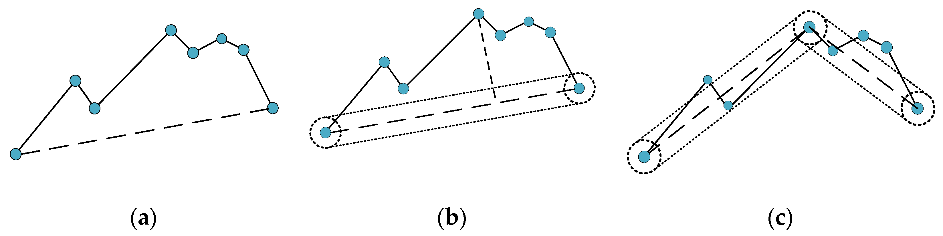
Step 1: Baseline Establishment. The algorithm commences by selecting the initial and terminal points of the trajectory as the pivotal baseline, which acts as a reference for the ensuing compression, depicted in Figure 2a.
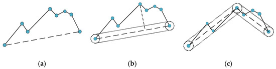
Figure 2.
Schematic diagram (a–c) of the principle of the DP algorithm.
Step 2: Perpendicular Distance Calculation. Subsequently, the algorithm computes the orthogonal distance from every point along the trajectory to the baseline. The point at the maximum distance is deemed the ‘key point’ for the current iteration, as illustrated in Figure 2b.
Step 3: Threshold Evaluation. This step involves comparing the orthogonal distance of the identified key point to a pre-established threshold to ascertain if it falls within the permissible margin of error.
Step 4: Trajectory Bifurcation. Should the key point’s perpendicular distance surpass the threshold, it is preserved as a critical juncture. The trajectory is then segmented at this juncture, subdividing the original path into two segments and thereby setting the stage for subsequent iterations, as showcased in Figure 2c.
Step 5: Iterative Refinement. The process enters a recursive phase, where Steps 2 through 4 are reiterated for each sub-trajectory. This recursive refinement continues until all points on the sub-trajectories lie within the acceptable distance threshold from their respective baselines.
A key characteristic of the DP algorithm is its ability to modulate the granularity of the compression via threshold manipulation. A diminutive threshold value ensures a compressed trajectory that closely mirrors the original dataset, preserving maximum fidelity. On the other hand, elevating the threshold value can lead to a more generalized representation, potentially omitting finer details in the process. Thus, the judicious selection of the threshold is critical, as it directly influences the balance between data integrity and compression in the application of the DP algorithm to trajectory data.
2.2. Enhancing the DP Algorithm for the Construction of a Hierarchical and Sequential Tree Structure for Ship Trajectory Point Compression
The classic DP algorithm traditionally employs a singular, experientially derived distance threshold to compress trajectories, which may not always optimally reflect the spatial intricacies of varying maritime environments. Particularly in complex maritime zones brimming with islands and reefs, the convoluted nature of ships’ pathways necessitates finer thresholds to preserve critical navigational points, ensuring the retention of trajectory resemblance. Conversely, the more uniform and predictable routes found in open sea regions can accommodate broader thresholds. However, the one-size-fits-all approach of the original DP algorithm can lead to an overgeneralization of trajectory data in intricate sea areas, possibly discarding vital navigational markers or, conversely, maintaining superfluous trajectory points in open waters, leading to data redundancy.
Addressing the shortcomings of a fixed-distance threshold approach, this paper innovates the field by constructing a tiered hierarchy of ship trajectory points, capitalizing on their distinctive attributes.
2.2.1. Stratifying Ship Trajectory Data into Hierarchical Levels
The quintessential strategy of DP-derived algorithms is the bifurcation of trajectories into segments that are delineated by points of maximum divergence from a baseline, which are then addressed recursively. This concept resonates with the foundational mechanisms of the multi-branch-tree pre-order construction algorithm [17]. Drawing inspiration from this, this paper harnesses the multi-branch-tree pre-order concept to facilitate a structured and layered approach to the processing of ship trajectories.
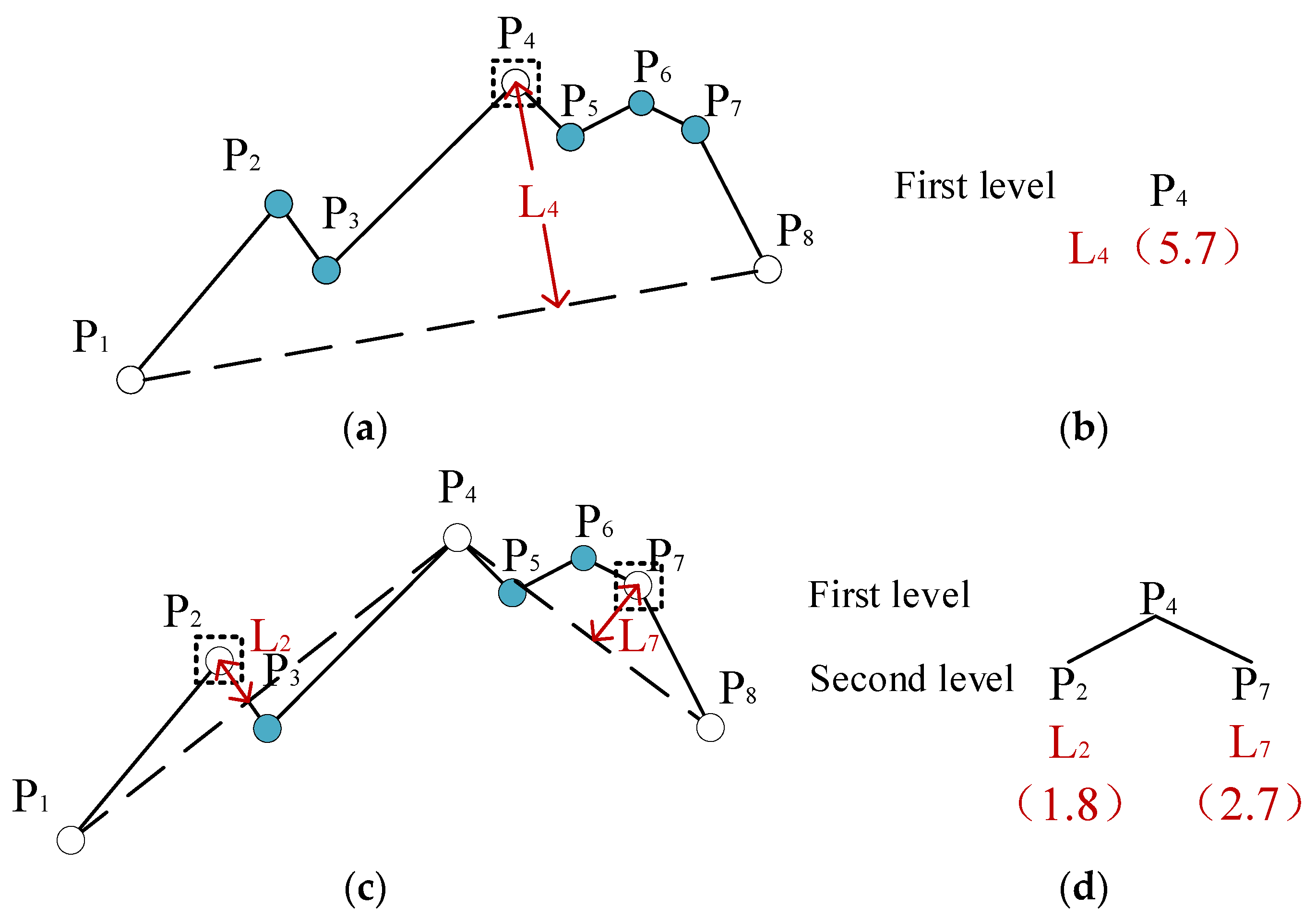
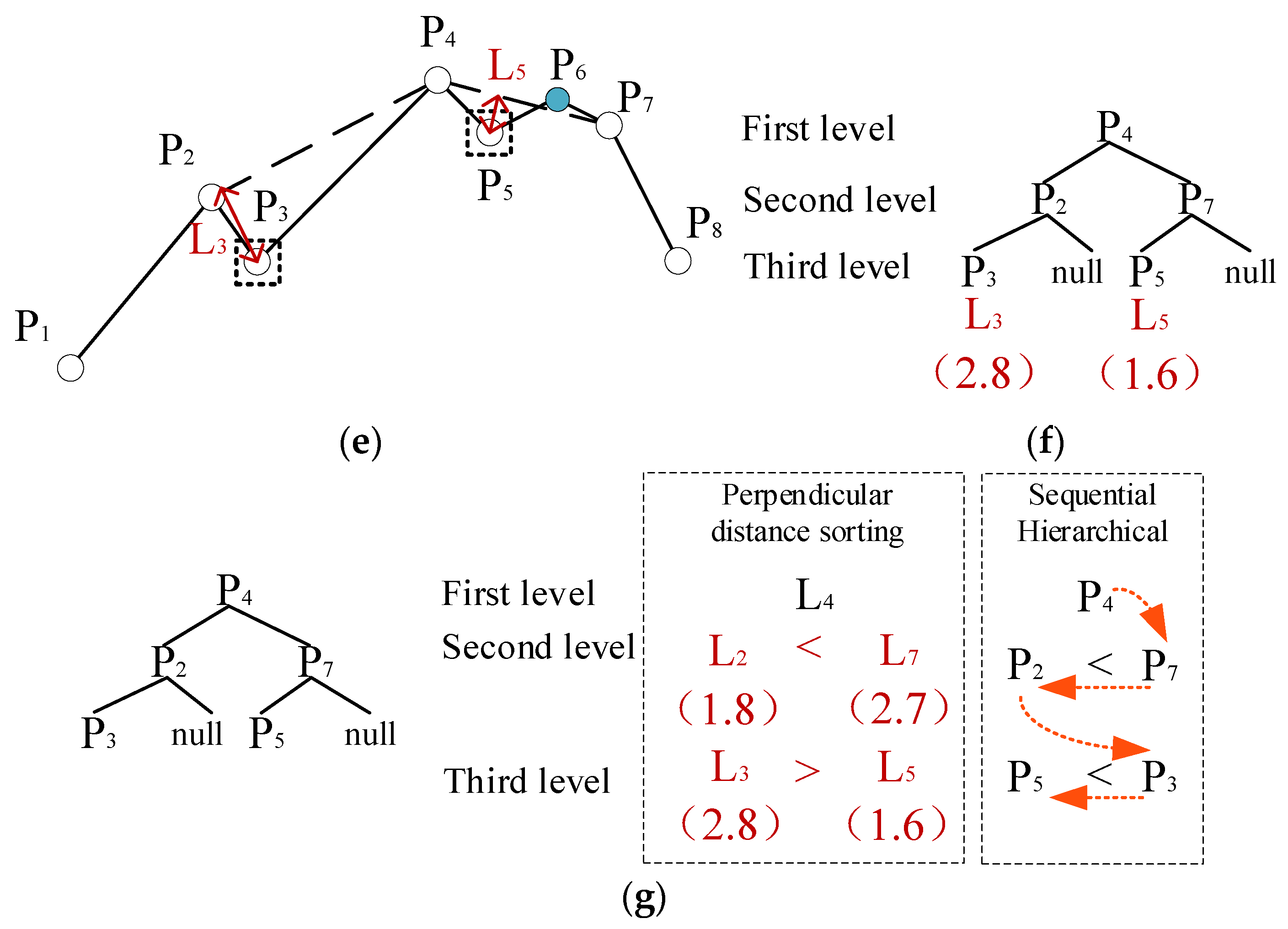
As illustrated in Figure 3a,b, the point of greatest perpendicular distance, point P4, is identified as the initial root node, establishing it as the primary tier and noting its perpendicular distance L4 (value 5.7); the trajectory is subsequently segmented at P4, as depicted in Figure 3c,d, thus positioning the points of the next greatest distances, P2 and P7, as P4’s offspring in the second tier, recording their respective distances L2 (value 1.8) and L7 (value 2.7); proceeding to Figure 3e,f, the process iteratively continues, dissecting at P2 and P7, with subsequent points along the sub-segments being classified into the third tier; this recursive execution persists until all points are integrated within the tree structure, with the recursion count defining each point’s hierarchical level.
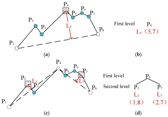
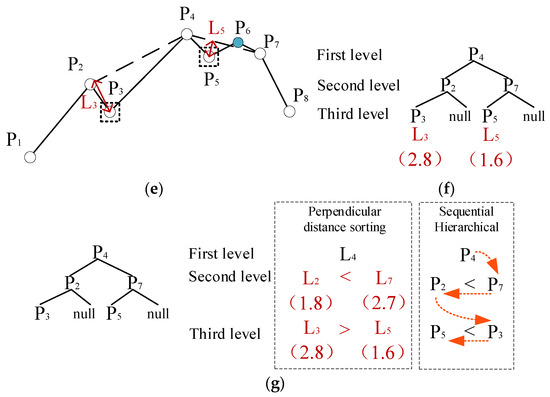
Figure 3.
Schematic diagram (a–g) of the hierarchy sequence tree for ships’ trajectory points.
2.2.2. The Grading of Trajectory Points at the Same Hierarchical Level
Once the trajectory points are systematically categorized within the tree structure, each node representing a trajectory point retains a record of both its hierarchical tier and the magnitude of its perpendicular distance. Subsequently, the tree is traversed utilizing a multi-branch-tree pre-order algorithm, cataloging nodes of identical tiers into a list; this culminates in the sorting of these lists by their perpendicular distances, as delineated in Figure 3g, with the arrows indicating the hierarchical flow from superior to subordinate tiers.
Upon the establishment of this hierarchical and sequential tree structure of the trajectory points, the algorithm facilitates a progressive refinement of points to be retained, advancing from the lower to the higher tiers. This method not only refines the spatial similarity across trajectories for effective compression but also dynamically aligns the compression process with the underlying geographical complexity of the ship routes.
2.3. Evaluation of Spatial Similarity in Ship Trajectories and Mining of Change Rules of the Hierarchy Sequence Tree
Trajectories can be constructed as line features composed of temporal points through preprocessing. The main methods for evaluating line feature similarity include:
(1) The Hausdorff Distance-Based Evaluation Method [18]: This method assesses similarity by evaluating the minimum distance between the compression nodes and the original trajectory. The principle of this method is clear and straightforward, focusing primarily on spatial location. However, in applications where point order or temporal information is essential, it often overlooks critical sequential information.
(2) The Fréchet Distance-Based Evaluation Method [19]: This method considers the positions and order of the trajectory points before and after compression. It primarily concerns the geometric shape of the curves rather than temporal information. If two trajectories are similar in shape but have temporal shifts, the Fréchet distance may not accurately reflect their similarity.
(3) The Dynamic Time Warping (DTW) Method [20,21]: DTW is an algorithm for processing time series data, characterized by its temporal elasticity matching capability, allowing it to find the best match between trajectories with time shifts or speed inconsistencies. This flexibility in handling time series data makes it particularly suitable for evaluating trajectory similarity with temporal factors.
Considering that the nodes, trajectory length, and time series of ship trajectories will change before and after compression and that the DTW algorithm can handle shape changes and length differences between time series while measuring their similarity, it is an ideal choice for evaluating ship trajectory similarity.
The DTW algorithm can be described mathematically as follows:
where X and Y are the two sequences (trajectories) that are being compared, d(xi, yj) represents the distance between points xi and yj, and K is the warping path length. The DTW distance is computed by finding the optimal alignment that minimizes the cumulative distance between the two sequences.
This paper selects four historical AIS trajectories as sample cases. By gradually reducing the number of trajectory points in the ship trajectories along the hierarchical sequence, the changes in two key indicators, similarity and the similarity gradient, are monitored throughout the compression process. These changes are plotted as the similarity transformation curves and absolute difference curves, as shown in Figure 4, to study the laws governing trajectory similarity changes during the compression of trajectory points.
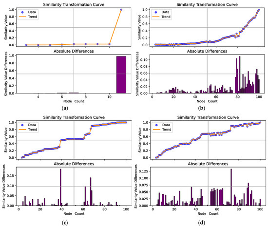
Figure 4.
Similarity variation graph of hierarchical and sequential trees for trajectory points. The graph is divided into subgraphs (a–d), each representing the similarity and similarity gradient curves for different AIS trajectory samples. The subgraphs provide a detailed view of how the similarity between the compressed and original trajectories changes as the number of trajectory points is reduced.
From the similarity and gradient curves in Figure 4, it can be seen that as the trajectory points are progressively compressed, the disparity between the compressed and original trajectories gradually increases. The similarity decreases as more points are discarded, leading to the gradual omission of some trajectory features.
During this process, the change in similarity is not always smooth. A significant drop in similarity can be observed when some important feature points in the trajectory are discarded, which is defined in this paper as the local step jump phenomenon, and these points are defined as step jump points. In the initial stages of compression along the hierarchical tree, the similarity changes calculated by DTW are more pronounced, especially around the step jump points. This is because the trajectory loses key feature points from its complete state, significantly reducing the similarity between the compressed trajectory and the original trajectory. After passing the maximum step jump, the rate of similarity change gradually slows down, reflecting that the difference between the compressed trajectory and the original trajectory has expanded to a certain extent, causing the subsequent compression to have an increasingly limited impact on the similarity.
Therefore, the maximum step jump is a crucial parameter in the trajectory compression process. This point can be used to guide the setting of the compression level to ensure that the key features of the trajectory are preserved as much as possible.
2.4. Adaptive Compression of Trajectories Using Maximum Step Points
In Section 2.3, the establishment of an optimal compression magnitude is identified as a fundamental factor for the effective compression of trajectory point sequences within a hierarchical structure. It is acknowledged that with the increase in compression level, there is a concomitant decrease in similarity, with the maximum step jump point emerging as a pivotal parameter in the trajectory compression framework. This parameter aids in calibrating the compression magnitude. Consequently, this study focuses on pinpointing the trajectory points exhibiting the most substantial jumps in similarity within the hierarchical sequence, subsequently omitting points below this threshold to achieve the desired compression.
The specific resolution process is as follows:
(1) Compute the Gradient of Change: Calculate the gradient of the DTW (dynamic time warping) computation values with respect to the number of points that are retained after compression. This can be expressed as:
where ΔDTW represents the change in DTW value and ΔN represents the change in the number of points retained.
(2) Analyze the Gradient Changes: Identify the points of significant mutation, where the DTW computation values experience the greatest change during the compression process. This can be determined by finding the local maxima in the gradient changes.
(3) Determine the Number of Retention Points: Identify the number of points to retain at the local maximum of the gradient change. This can be mathematically formulated as:
where Nretained is the number of points to be retained after compression.
(4) Compression Implementation: Using Nretained as the number of points to retain, remove those points in the original trajectory that correspond to secondary features. The goal is to preserve the essential characteristics of the trajectory as much as possible after compression.
In this formula, T represents the original set of trajectory points and Tcompressed denotes the trajectory after compression, with the amplitude defined by Nretained.
By selecting Nretained as the number of points to retain, one could remove the points in T that correspond to secondary features, aiming to preserve the essential characteristics of the trajectory as much as possible after compression.
3. Results and Discussion
3.1. Background
This paper selects AIS trajectory data from different types of vessels, including cargo ships, oil tankers, and fishing vessels (catching boats), to use as case studies. Each trajectory contains dynamic information such as timestamps, geographical coordinates (latitude and longitude), speed over ground, and course, as well as static information such as the Maritime Mobile Service Identity (MMSI) number, vessel name, and vessel length.
The case study is divided into two main parts: the first part consists of testing the effectiveness of the algorithm’s self-adaptive trajectory compression with a small number of trajectories; then, the universality of the algorithm for self-adaptive trajectory compression under different conditions is evaluated with a larger sample.
The classic ship trajectory compression method based on threshold setting considers safety and seaworthiness issues. Through statistical study, the threshold baseline for the Douglas–Peucker (DP) compression method was chosen to be 0.8 times the vessel length [13]. This vessel domain DP compression method (hereinafter referred to as the VD-DP method) is widely adopted in current research [14] and was therefore chosen as the comparative method for this paper (hereinafter referred to as SACST, self-adaptive compression for ship trajectory).
3.2. Case Study I: Small-Sample Trajectory Compression
Differences exist in the trajectories of various types of vessels. Fishing vessels may exhibit complex and variable trajectories due to frequent changes in course during fishing activities. In contrast, cargo ships typically navigate along fixed shipping lanes, resulting in relatively stable trajectories, while oil tankers, due to their heavier loads and larger size, usually move more slowly and make fewer turns. To verify the capability of the proposed method (SACST) to handle multi-type trajectory data, this study utilizes real voyage data from two cargo ships, two oil tankers, and two fishing vessels recorded by the AIS in the Yellow and Bohai Seas on 1 August 2019 for testing. The basic information on these trajectories, including trajectory name, type of vessel, MMSI code, and the number of trajectory points, is detailed in Table 1.

Table 1.
Basic information on the small-sample trajectory data.
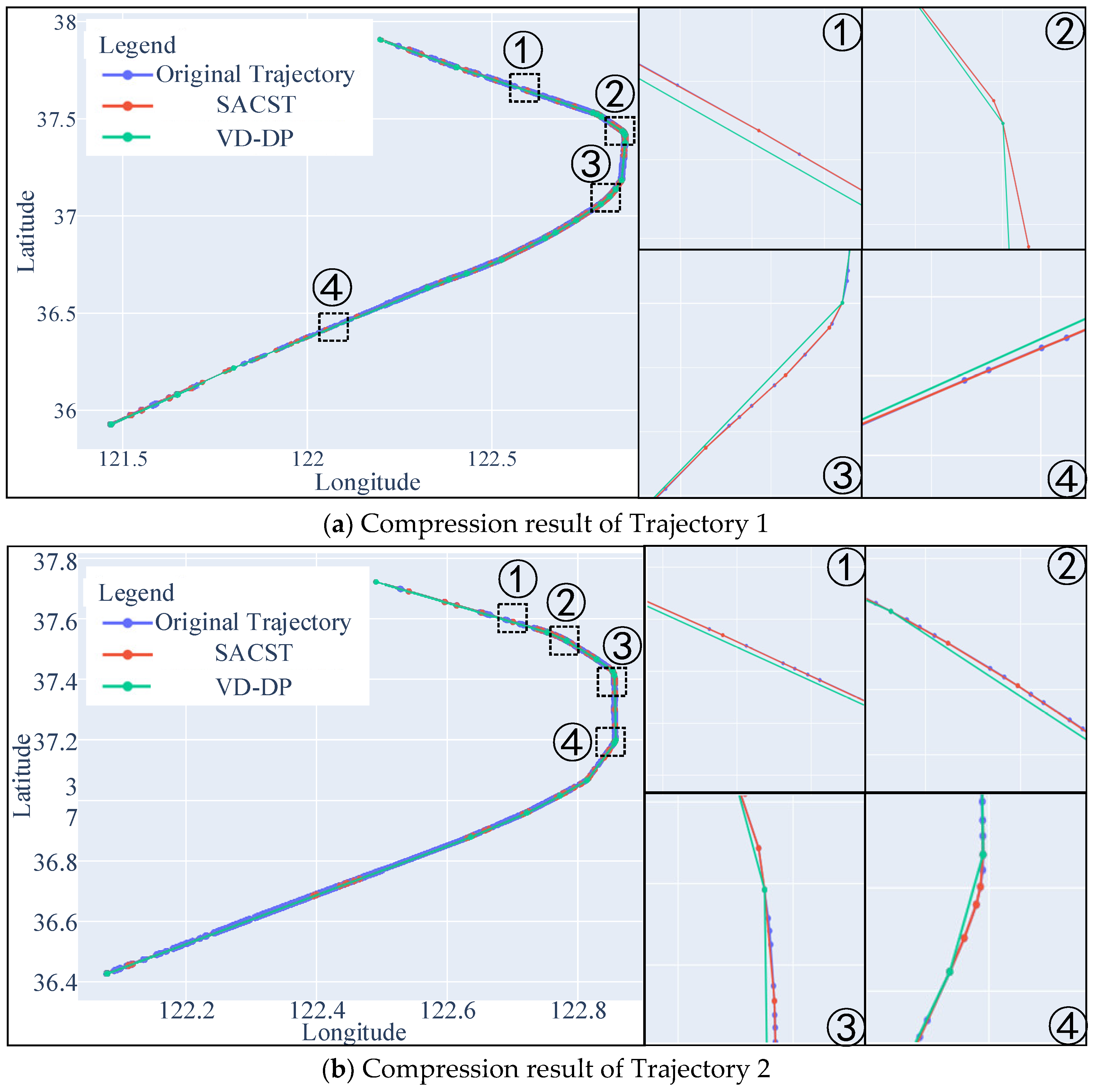
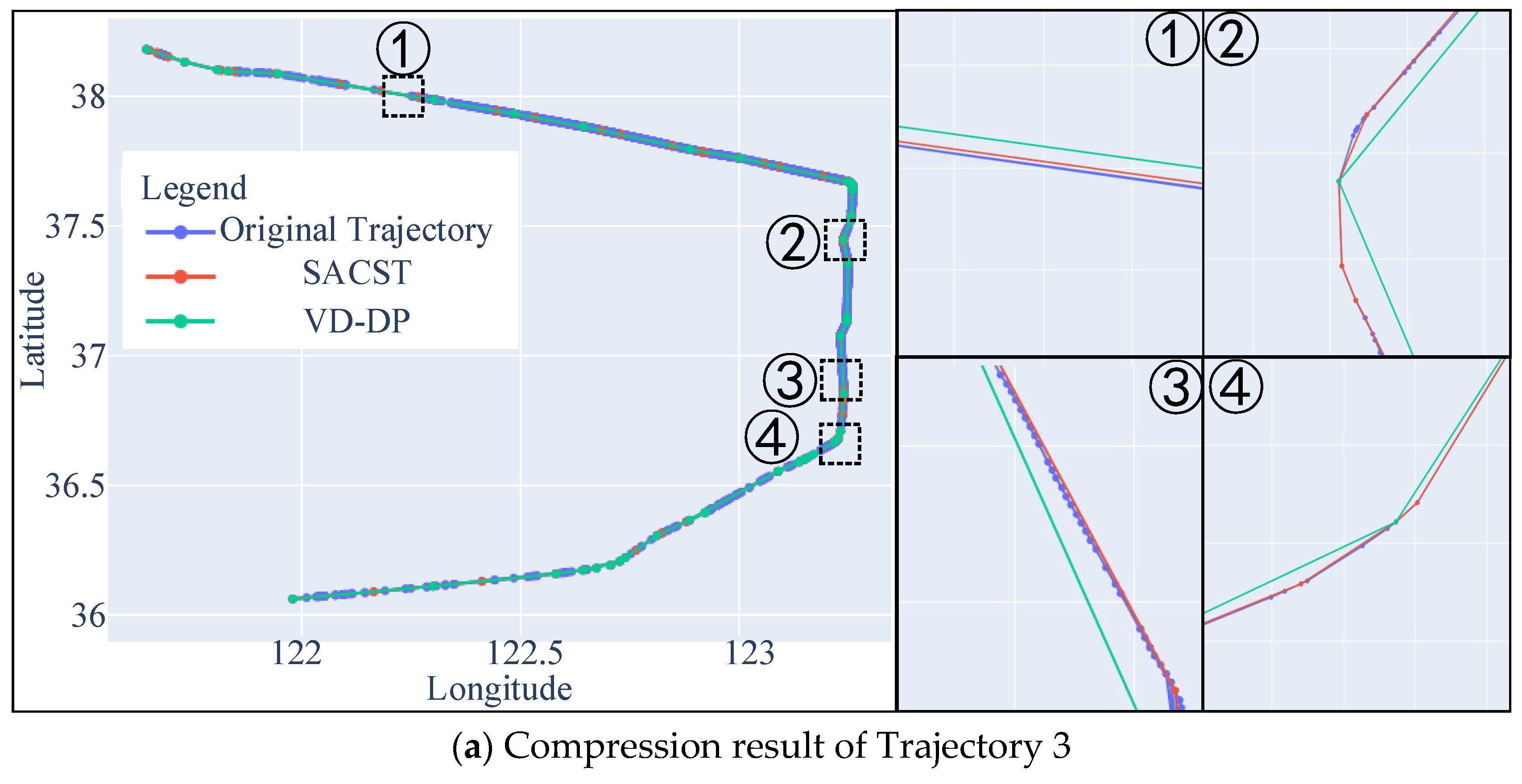
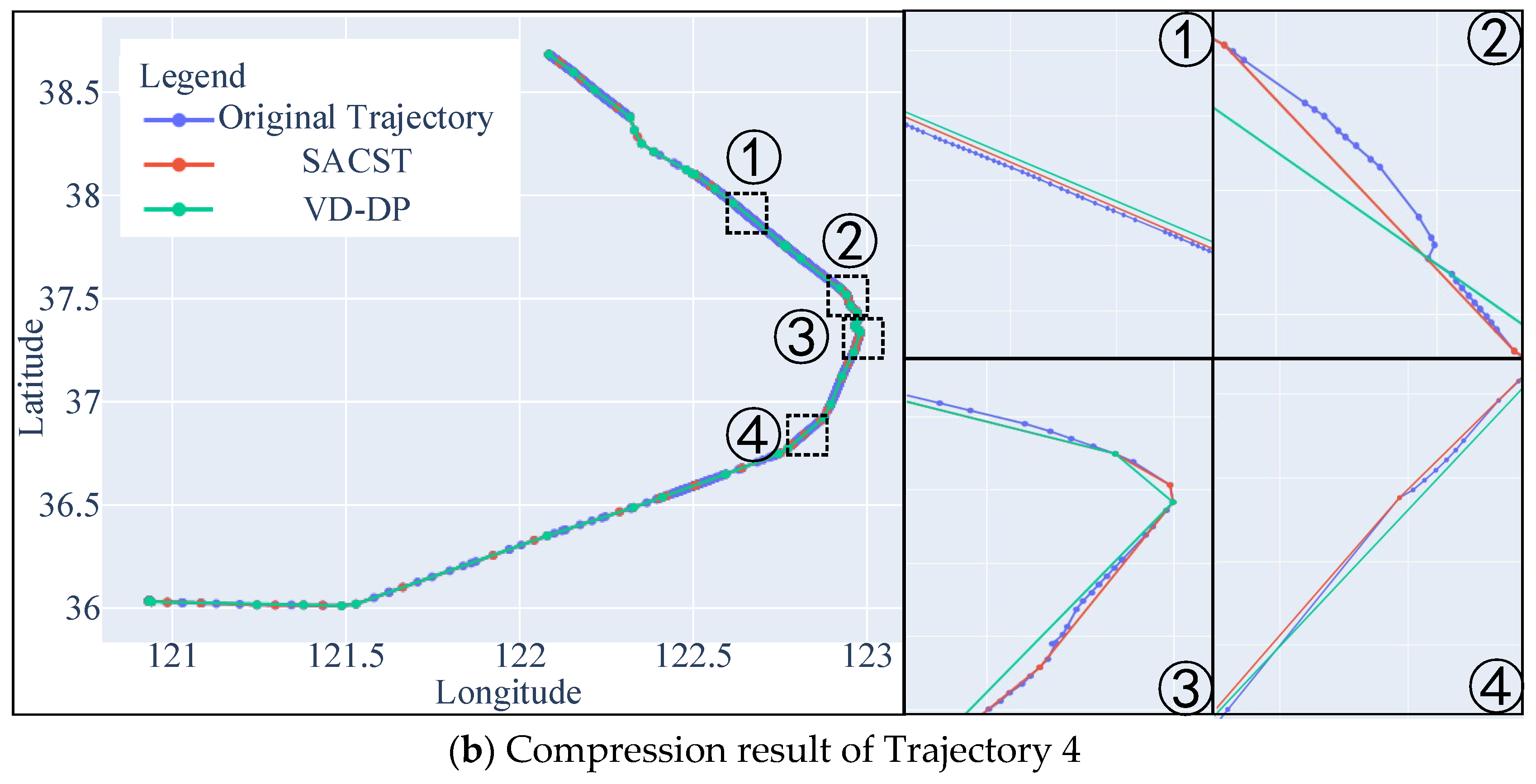
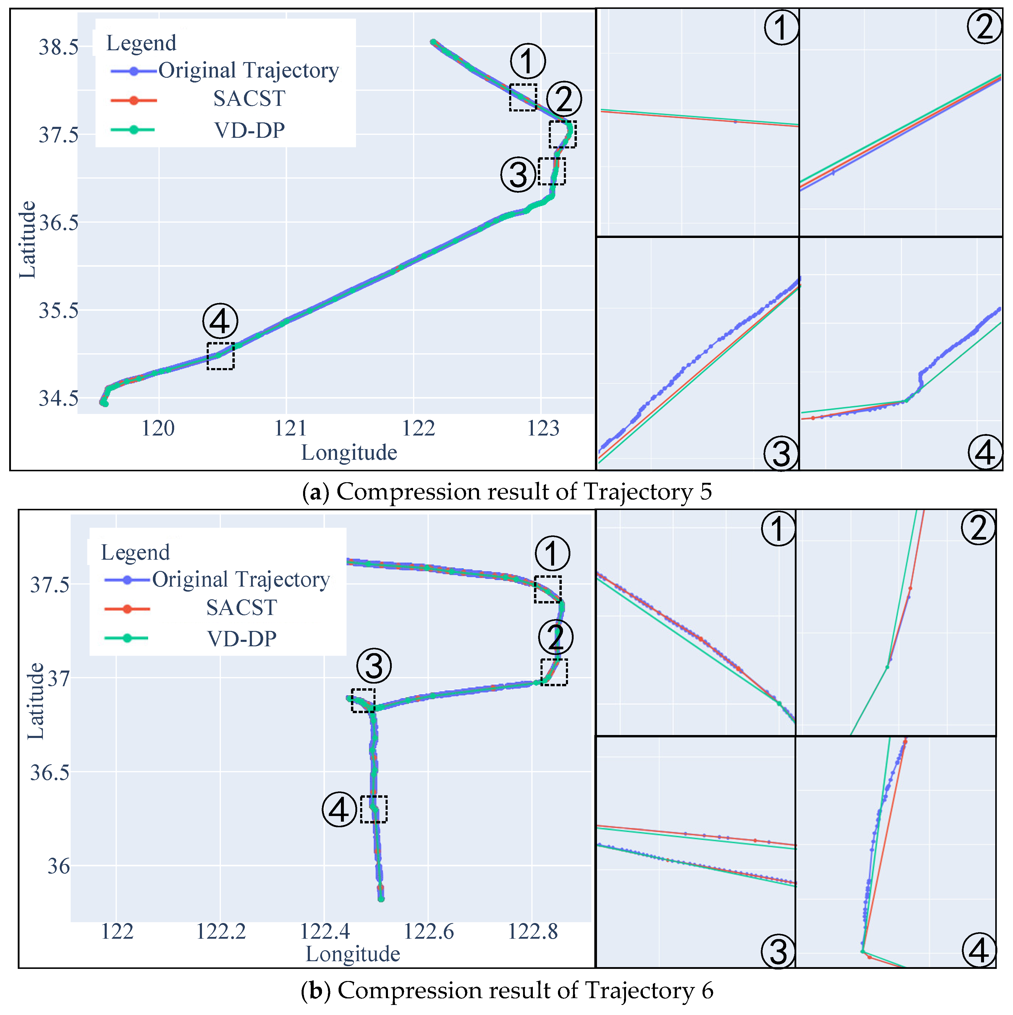
The case study compresses Trajectories 1–6 using both SACST and VD-DP. Figure 5 illustrates the compressed trajectories of a fishing vessel; Figure 6 presents the trajectory of a cargo ship; and Figure 7 shows the trajectory of an oil tanker. The original trajectories are represented by blue polylines, those processed by SACST are represented by a red polyline, and those processed by VD-DP are represented by a green polyline.
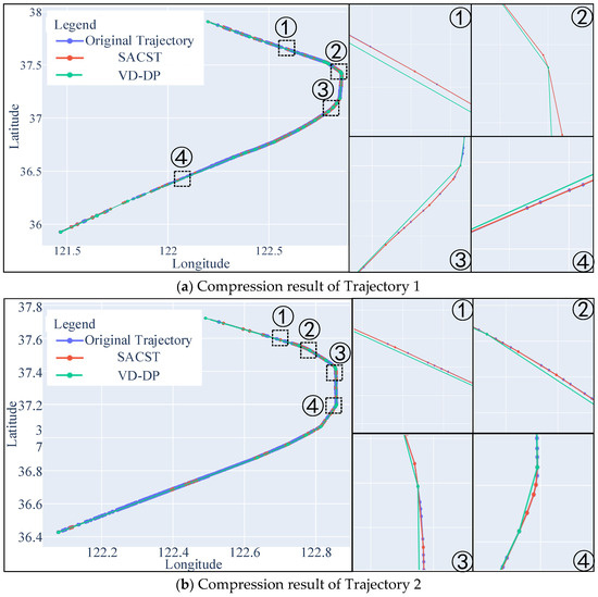
Figure 5.
Schematic diagram of fishing vessel trajectory compression.
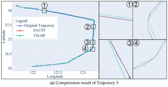
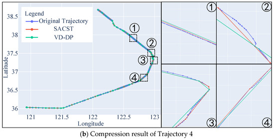
Figure 6.
Schematic diagram of cargo ship trajectory compression.
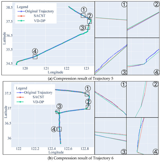
Figure 7.
Schematic diagram of oil tanker trajectory compression.
The visual comparison of the trajectories indicates that the ship trajectories generated by SACST match the original trajectories more closely. In the magnified diagrams ①②③④ of Figure 5, Figure 6 and Figure 7, the trajectories compressed using the self-adaptive compression ship trajectory (SACST) method, depicted in red, are predominantly closer in spatial proximity to their original counterparts (illustrated in blue) compared to those compressed by the variable densification–Douglas–Peucker (VD-DP) algorithm, represented in green. This proximity is particularly evident at locations with pronounced change features, such as turning points. This demonstrates that SACST can preserve the detailed features of the original trajectories after compression more effectively.
To quantitatively validate the superior performance of SACST, this paper employs two key metrics: the compression ratio (CR), which measures the reduction in trajectory points through compression, and dynamic time warping (DTW), a measure of the trajectory similarity before and after simplification. The compressed trajectories from both algorithms are compared with the original trajectories for analysis. The results are presented in Table 2.
Table 2.
Statistical data on parameters for small-sample trajectory compression results.
As indicated in Table 2, for the fishing and cargo ship trajectories (Trajectories 1–4), the compression ratio of SACST is slightly lower than that of VD-DP; however, it remains fundamentally consistent. Nevertheless, the DTW values between the compressed and original trajectories using SACST significantly decrease compared to VD-DP, with a 75.7% reduction for Trajectory 1, a 64.03% reduction for Trajectory 2, a 42.25% reduction for Trajectory 3, and a 21.16% reduction for Trajectory 4. These results demonstrate that SACST, while ensuring compression efficiency, is better at preserving the original characteristics of the trajectory, significantly enhancing the similarity of the compressed trajectory.
The compression indicators for Trajectory 6 of the oil tanker are largely consistent with the aforementioned results. However, there is a discrepancy with Trajectory 5, where the DTW value of SACST is slightly higher than that of VD-DP, with an increase of 0.29%. A visual comparison of the trajectories compressed by the two methods, as depicted in Figure 7a(①②③④), reveals that they are essentially identical. This suggests that for the less maneuverable and more uniform characteristics of oil tanker trajectories, the proposed method may achieve effects that are practically comparable to the comparative method under certain conditions.
In conclusion, the SACST method not only maintained a high compression ratio when compressing ship trajectories under various types of vessels and navigation conditions, but also significantly improved the spatial similarity compared to the VD-DP method. This indicates that SACST can adaptively compress trajectories with greater precision and effectiveness, based on their specific characteristics, without relying on the setting of parameter thresholds.
3.3. Case Study II: Large-Sample Trajectory Compression
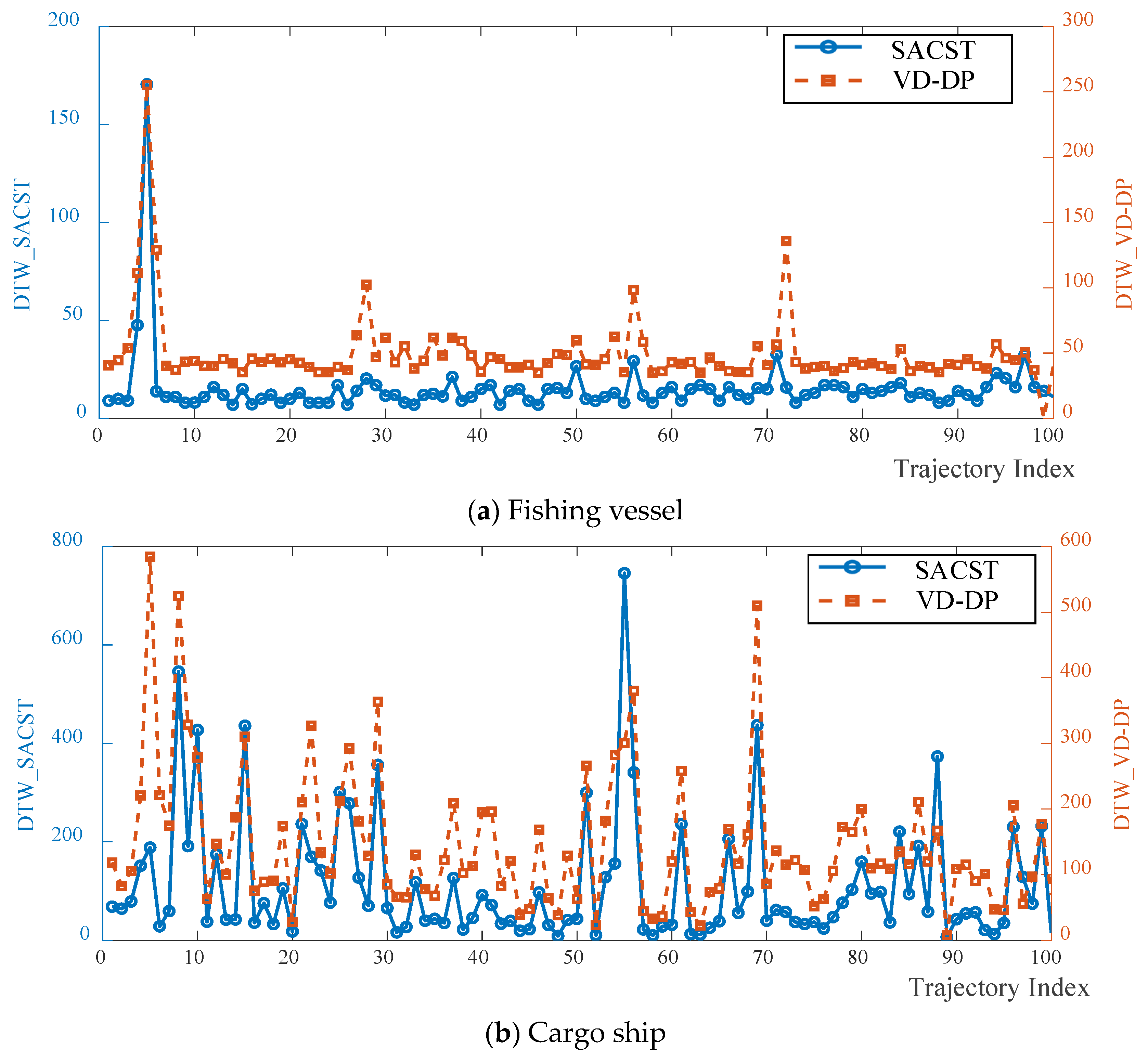
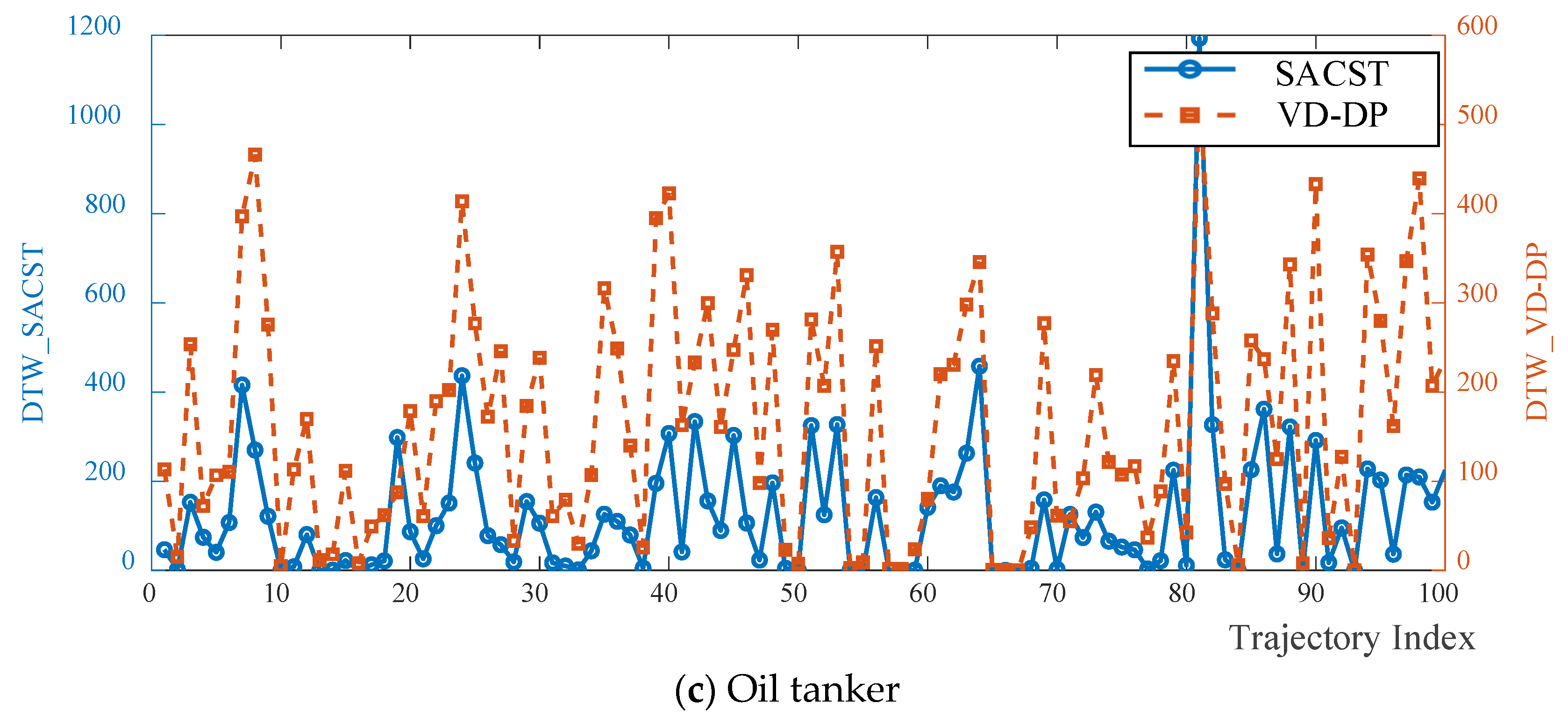
This section is dedicated to validating the universality of SACST in self-adaptive trajectory compression through an extensive trajectory compression case study on a large sample set. The selected sample set comprises 100 vessel trajectories for each of the three different types: fishing boats, cargo ships, and oil tankers. The sample set represents vessel trajectories that passed through ports, reef areas, and open waters in the Yellow and Bohai Seas on 1 August 2019, ensuring the wide applicability of the case study data. Figure 8 presents the similarity comparison curves between the SACST and VD-DP trajectory compression methods, where similarity is measured using the DTW value, with a smaller DTW value indicating greater similarity between the compressed and original trajectories. Specifically, Figure 8a illustrates the DTW curve for the compressed trajectory of a fishing vessel, Figure 8b shows the DTW curve for the compressed trajectory of a cargo ship, and Figure 8c presents the DTW curve for the compressed trajectory of an oil tanker. It can be observed from Figure 8 that, regardless of whether they are for fishing vessels, cargo ships, or oil tankers, the DTW curves generated by the SACST method are, in the vast majority of cases, positioned below those generated by the VD-DP method, demonstrating that SACST performs better in maintaining trajectory similarity.
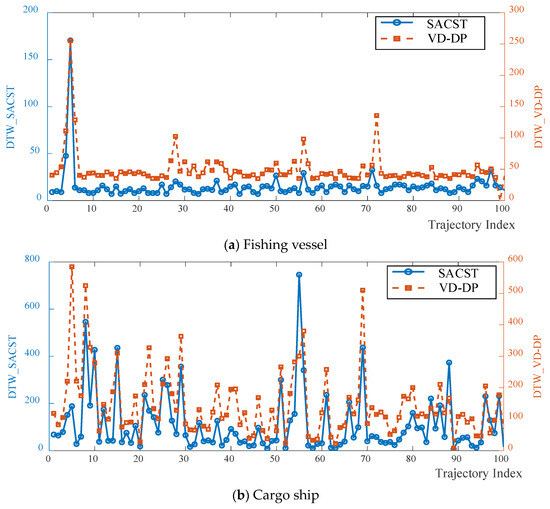
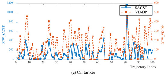
Figure 8.
Similarity comparison curve for ship trajectory compression.
The detailed statistical data on the effects of trajectory compression are presented in Table 3. The table lists two main trajectory compression techniques, VD-DP and SACST, and compares their performance in terms of their compression ratio (CR) and dynamic time warping (DTW) values when processing the trajectory data of three different types of vessels: fishing vessels, cargo ships, and oil tankers. Through this comparison, it is possible to clearly assess the efficiency and similarity preservation capabilities of both methods when dealing with trajectory data from different types of ships.
Table 3.
Statistical data on parameters for large-sample trajectory compression results.
The results of the trajectory compression on a large scale indicate that for fishing vessel trajectories, the DTW values between the trajectories compressed by the method proposed in this paper and the original trajectories decreased significantly compared to those of the comparative method, showing a reduction of 70.3%. For cargo ship trajectories, the DTW values using the proposed method showed a decrease of 19.7% compared to the comparative method; for oil tanker trajectories, there was a reduction of 19.8%. These findings demonstrate that for the complex and variable trajectories of fishing vessels, the method proposed in this paper better accounts for the spatial structural characteristics of the trajectories, significantly improving data compression accuracy while maintaining a basic compression rate. However, for the relatively stable trajectories of cargo ships and oil tankers, the room for improvement in compression effects is relatively limited. Although the method proposed also enhances the data compression accuracy, the magnitude of the improvement is not as significant as the effects seen in the compression of fishing vessel trajectories.
Moreover, in contrast with the comparative method, which requires the input of empirical threshold values, the proposed method adaptively determines the compression extent directly based on the spatial structural features of the trajectory. During the case study, there was no need to preset threshold parameters, which also efficiently addresses the issue of the potential lack of universality in empirical parameter thresholds.
4. Conclusions
To address the limitations of existing methods for ship trajectory compression, which rely on fixed thresholds that are empirically set and encounter challenges in maintaining spatial similarity both before and after compression, this paper proposes a self-adaptive compression method for ship trajectories without threshold setting. Through theoretical analysis and case study validation, the main conclusions reached are as follows:
- (1)
- The method proposed in this paper, known as SACST, has demonstrated superior performance in compression, effectively retaining the intricate details of the original ship trajectories. The visual comparative analysis and numerical validation data from Case Study I indicate that the trajectories after compression by means of SACST exhibit a higher degree of spatial similarity to the original trajectories compared to those compressed using the VD-DP algorithm, particularly at points with pronounced change features, such as turning points.
- (2)
- In the case of trajectory compression with large sample sets, compared to the VD-DP method, SACST reduced the DTW calculation value between the compressed and original trajectories by 25%, significantly enhancing the spatial similarity of the post-compression trajectories. This achievement is attributed to SACST’s ability to adaptively adjust the compression thresholds based on trajectory characteristics, accommodating various types and navigational states of ship trajectories, and thereby achieving a notable increase in spatial similarity across large-scale samples.
- (3)
- SACST could self-adaptively compress ships’ trajectories across various types of vessels and navigational conditions at high quality, showing broad application potential. SACST provides a comprehensive solution to alleviate the storage burden of raw AIS data for maritime surveillance platforms, which is anticipated to improve the efficiency and accuracy of maritime safety management and data oversight.
However, the introduction of spatial similarity analysis calculations did increase the computational load to a certain extent. Optimizing efficiency in computation time and resource usage for large datasets remains a challenge for future research.
Author Contributions
Conceptualization, Y.Z., L.Z., L.T., S.J. and Z.D.; methodology, Y.Z., L.Z. and L.T.; validation, Y.Z. and L.Z.; writing—original draft preparation, Y.Z. and L.Z.; visualization, Y.Z.; supervision, Y.Z. and L.Z.; funding acquisition, L.Z. All authors have read and agreed to the published version of the manuscript.
Funding
This work was supported by the National Natural Science Foundation of China under grants 41871369, 41901320, and 42071439.
Institutional Review Board Statement
Not applicable.
Informed Consent Statement
Not applicable.
Data Availability Statement
The data presented in this study are available from the corresponding author upon request. The data are not publicly available due to military sensitivity.
Conflicts of Interest
The authors declare no conflicts of interest.
References
- BS Pd IEC PAs: 61174-1:2021; Maritime Navigation and Radiocommunication Equipment and Systems. British Standards Institution: London, UK, 2021.
- Zhao, L.; Shi, G. A Method for Simplifying Ship Trajectory Based on Improved Douglas–Peucker Algorithm. Ocean Eng. 2018, 166, 37–46. [Google Scholar] [CrossRef]
- Robards, M.D.; Silber, G.; Adams, J.; Arroyo, J.; Lorenzini, D.; Schwehr, K.; Amos, J. Conservation Science and Policy Applications of the Marine Vessel Automatic Identification System (AIS)—A Review. Bull. Mar. Sci. 2016, 92, 75–103. [Google Scholar] [CrossRef]
- Bellman, R. On the approximation of curves by line segments using dynamic programming. Commun. Assoc. Comput. Mach. 1961, 4, 284. [Google Scholar] [CrossRef]
- Douglas, D.H.; Peucker, T.K. Algorithms for the reduction of the number of points required to represent a digitized line or its caricature. Cartogr. Int. J. Geogr. Inf. Geovisualization 1973, 10, 112–122. [Google Scholar] [CrossRef]
- Keogh, E.; Chu, S.; Hart, D.; Pazzani, M. An online algorithm for segmenting time series. In Proceedings of the IEEE International Conference on Data Mining, San Jose, CA, USA, 29 November–2 December 2001; pp. 289–296. [Google Scholar]
- Gao, M.; Guoyou, S.; Weifeng, L. Online compression algorithm of AIS trajectory data based on an improved sliding window. J. Traffic Transp. Eng. 2018, 18, 218–227. [Google Scholar] [CrossRef]
- Panagiotakis, C.; Pelekis, N.; Kopanakis, I. Segmentation and sampling of moving object trajectories based on representativeness. IEEE Trans. Knowl. Data Eng. 2012, 24, 1328–1343. [Google Scholar] [CrossRef]
- Visvalingam, M.; Whyatt, J.D. Line generalization by repeated elimination of points. In Landmarks in Mapping; Routledge: London, UK, 2017; pp. 144–155. [Google Scholar]
- Muckell, J.; Hwang, J.-H.; Lawson, C.T.; Ravi, S.S. Algorithms for Compressing GPS Trajectory Data: An Empirical Evaluation. In Proceedings of the 18th SIGSPATIAL International Conference on Advances in Geographic Information Systems (GIS 2010), San Jose, CA, USA, 2–5 November 2010; pp. 402–405. [Google Scholar] [CrossRef]
- Gao, M.; Shi, G.Y. Ship Spatiotemporal Key Feature Point Online Extraction Based on AIS Multi-sensor Data Using an Improved Sliding Window Algorithm. Sensors 2019, 19, 2706. [Google Scholar] [CrossRef] [PubMed]
- Li, Y.; Liu, R.W.; Liu, J.; Huang, Y.; Hu, B.; Wang, K. Trajectory Compression-Guided Visualization of Spatio-temporal AIS Vessel Density. In Proceedings of the 8th International Conference on Wireless Communications y Signal Processing (WCSP), Yangzhou, China, 13–15 October 2016; Volume 2016, pp. 1–5. [Google Scholar] [CrossRef]
- Zhang, S.K.; Liu, Z.J.; Cai, Y.; Wu, Z.L.; Shi, G.Y. AIS Trajectories Simplification and Threshold Determination. J. Navig. 2016, 69, 729–744. [Google Scholar] [CrossRef]
- Wei, Z.; Xie, X.; Zhang, X. AIS Trajectory Simplification Algorithm Considering Ship Behaviours. Ocean Eng. 2020, 216, 107086. [Google Scholar] [CrossRef]
- Yan, H. Spatial Similar Relationships; Science Press: Beijing, China, 2022. (In Chinese) [Google Scholar]
- Wang, R.; Yan, H.W.; Lu, X.M. Automation of the Douglas-Peucker Algorithm Based on Spatial Similarity Relations. Geogr. Inf. Sci. 2021, 23, 1767–1777. [Google Scholar]
- Cormen, T.H.; Leiserson, C.E.; Rivest, R.L.; Stein, C. Introduction to Algorithms, 3rd ed.; MIT Press: Cambridge, MA, USA, 2009. [Google Scholar]
- Chehreghan, A.; Ali Abbaspour, R. An assessment of the efficiency of spatial distances in linear object matching on multi-scale, multi-source maps. Int. J. Image Data Fusion 2018, 9, 95–114. [Google Scholar] [CrossRef]
- Buchin, K.; Löffler, M.; Ophelders, T.; van Renssen, A. Computing the Fréchet distance between uncertain curves in one dimension. Comput. Geom. 2023, 109, 101923. [Google Scholar] [CrossRef]
- Rakthanmanon, T.; Campana, B.; Mueen, A.; Batista, G.; Westover, B.; Zhu, Q.; Zakaria, J.; Keogh, E. Searching and Mining Trillions of Time Series Subsequences under Dynamic Time Warping; Academic Medicine: Cambridge, MA, USA, 2012; pp. 262–270. [Google Scholar] [CrossRef]
- Wang, L.; Koniusz, P. Uncertainty-DTW for Time Series and Sequences. In Computer Vision—ECCV 2022; Springer: Cham, Switzerland, 2022; pp. 176–195. [Google Scholar] [CrossRef]


Disclaimer/Publisher’s Note: The statements, opinions and data contained in all publications are solely those of the individual author(s) and contributor(s) and not of MDPI and/or the editor(s). MDPI and/or the editor(s) disclaim responsibility for any injury to people or property resulting from any ideas, methods, instructions or products referred to in the content. |
© 2024 by the authors. Licensee MDPI, Basel, Switzerland. This article is an open access article distributed under the terms and conditions of the Creative Commons Attribution (CC BY) license (https://creativecommons.org/licenses/by/4.0/).