
Node Load and Location-Based Clustering Protocol for Underwater Acoustic Sensor Networks

Abstract
1. Introduction
- (1)
- We propose a node load and location-based cluster member number optimization mechanism. Load determines the length of time slots required for channel access, while location affects the efficiency of channel access. By analyzing the impact of cluster member numbers on congestion based on node load and location information, we derive constraints on the maximum cluster member. Finally, the network complexity is reduced by maximizing the number of cluster members without congestion.
- (2)
- We propose a node degree and location-based cluster member selection mechanism to reduce network complexity by increasing the average number of cluster members. Firstly, the average number of cluster members is improved by removing nodes with node degree less than the maximum number of cluster members to avoid clusters with very few cluster members. Then, based on location, nodes farthest from the cluster head are removed to increase cluster cohesion. Thereby, the maximum number of cluster members that can be accommodated in a cluster is increased by enhancing the upper limit of intra-cluster information transmission.
- (3)
- We propose an novel priority-based clustering mechanism. Nodes are assigned cluster priority based on the maximum cluster member constraint without congestion. This approach ensures that as many clusters as possible have a number of cluster members close to the maximum, thus reducing the total cluster number after clustering completion. Ultimately, the purpose of maximizing the reduction of network complexity without congestion is achieved.
2. Related Work
2.1. Related Work
2.2. Problem Statement
3. LLCP
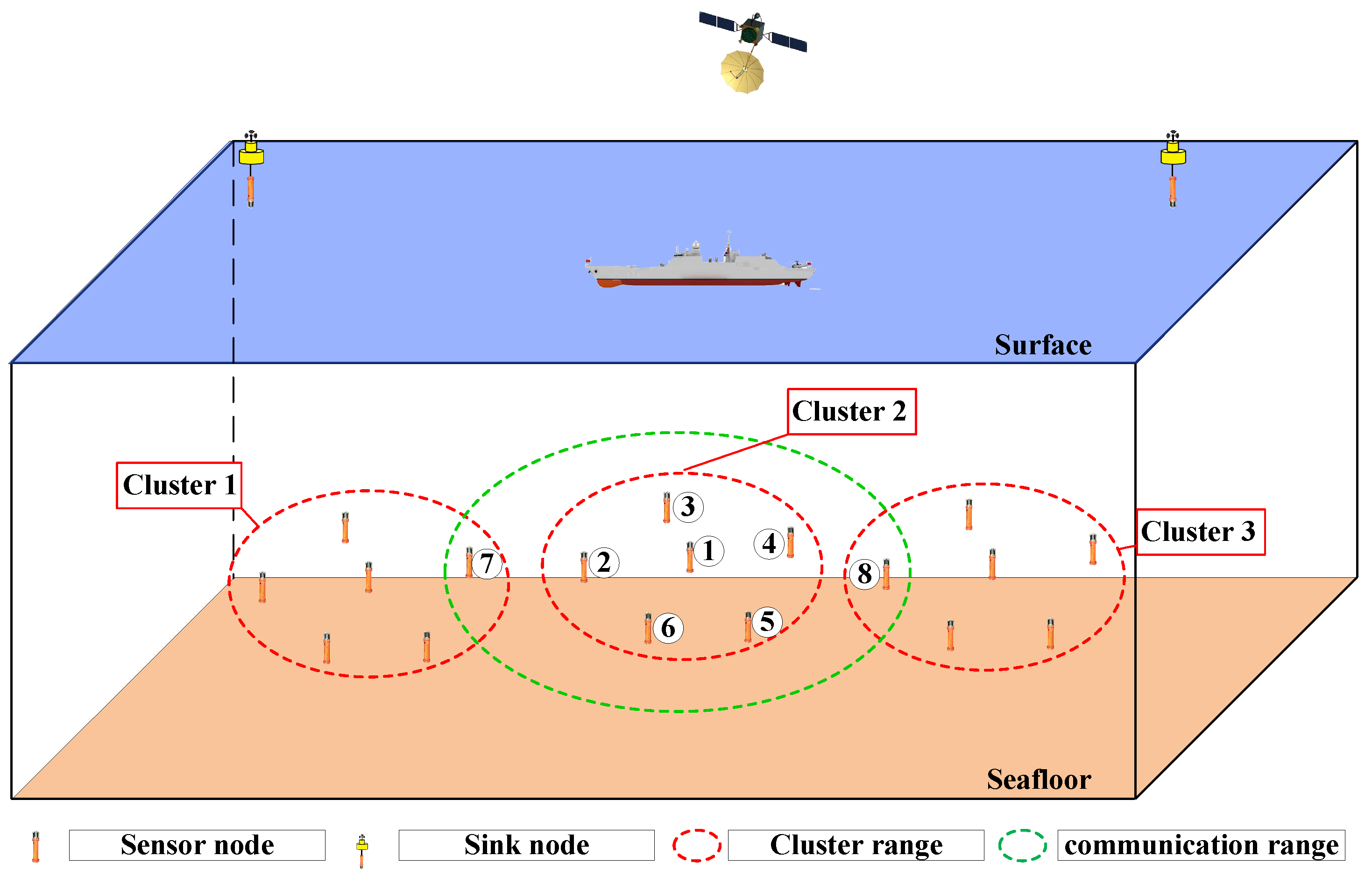
3.1. Network Modem
3.2. Frame Structure
3.3. Node Load and Location-Based Cluster Member Number Optimization Mechanism
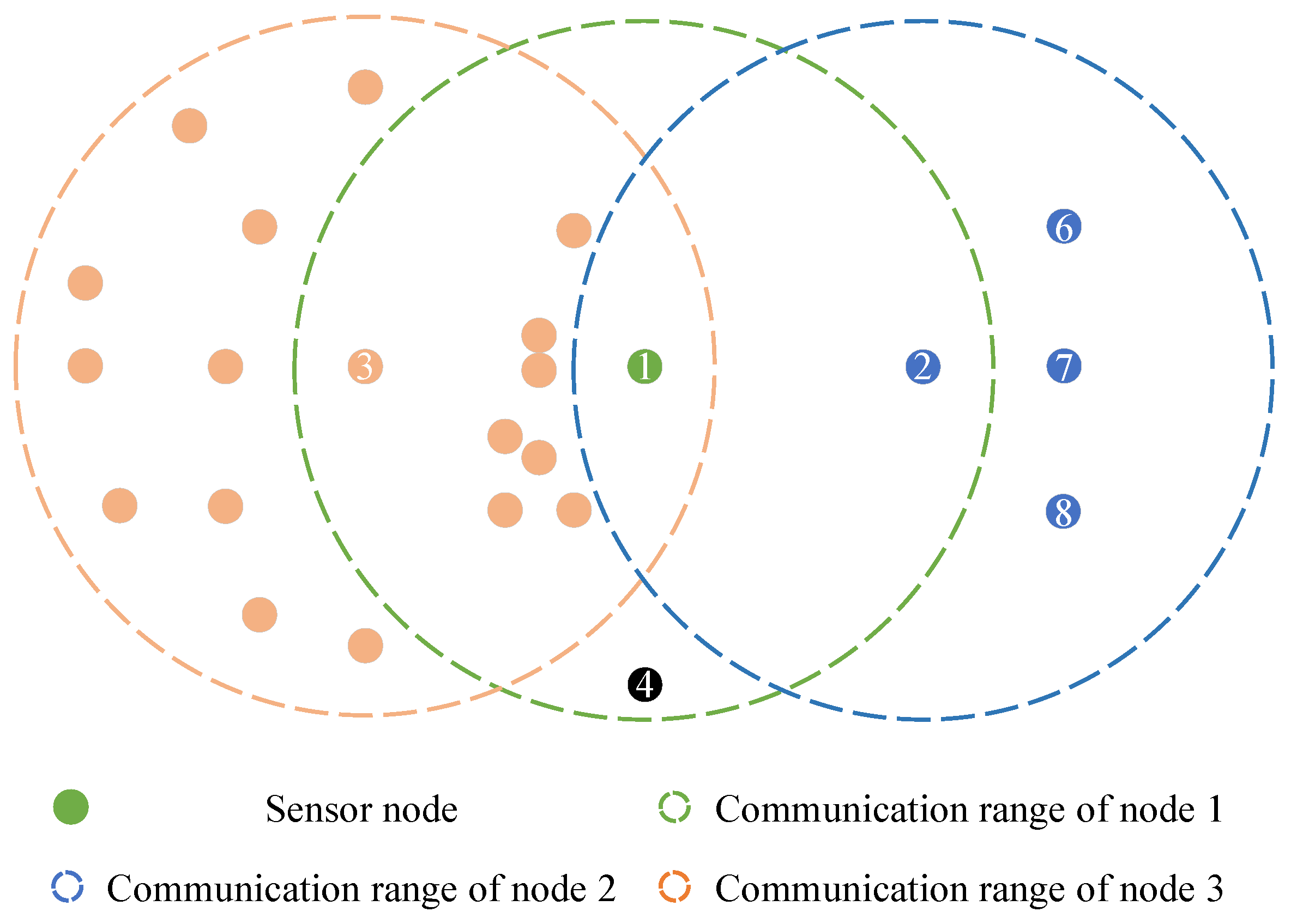
3.4. Node Degree and Location-Based Cluster Member Selection Mechanism
| Algorithm 1 Cluster Member Selection Algorithm Based on Node Degree and Location |
|
3.5. Priority-Based Clustering Mechanism
| Algorithm 2 Cluster Algorithm |
|
4. Simulation
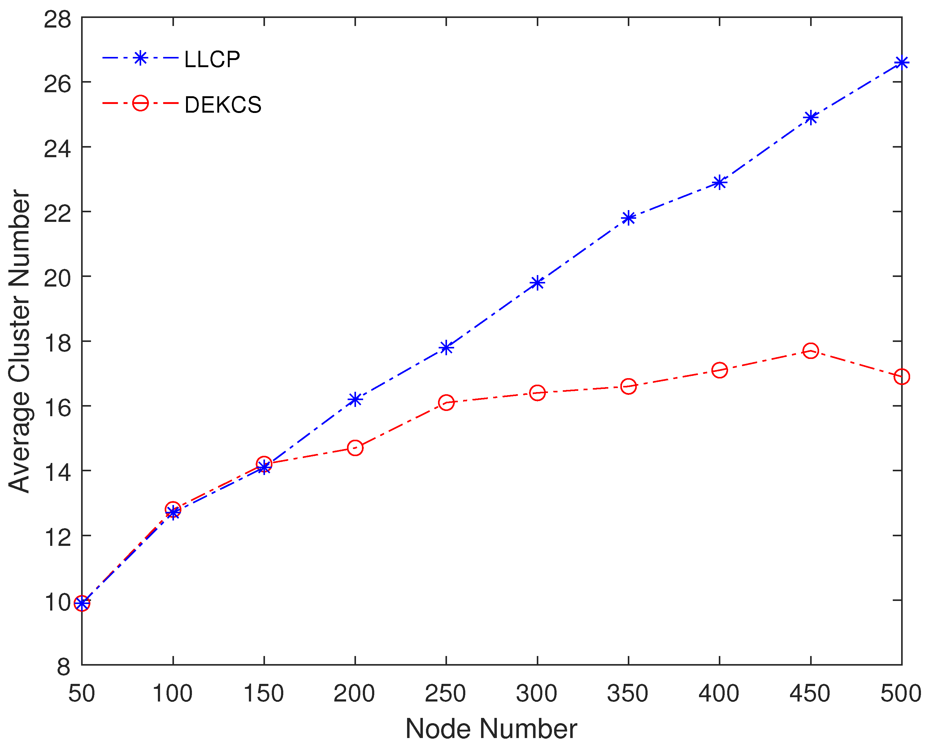
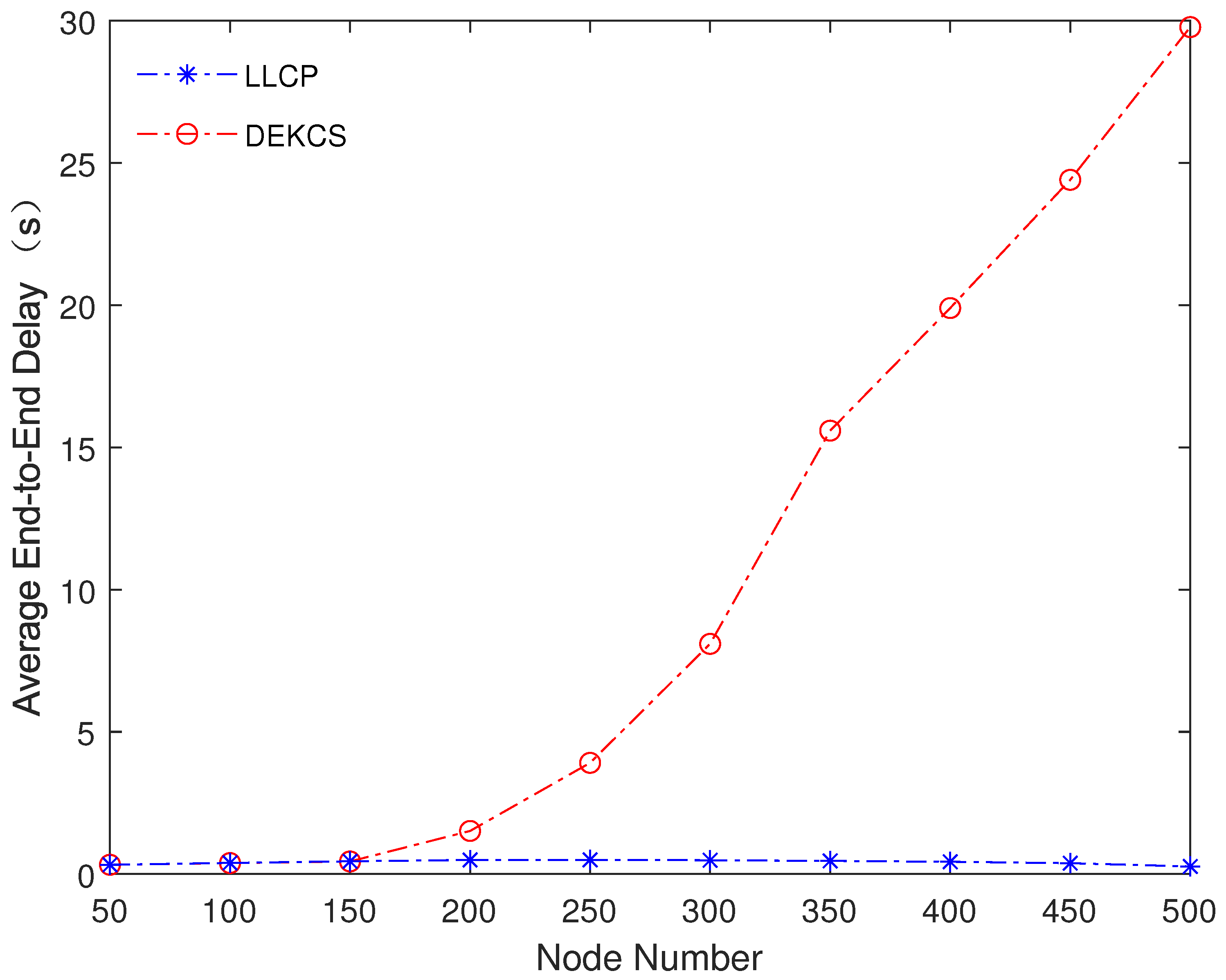
4.1. Performance under Different Node Numbers
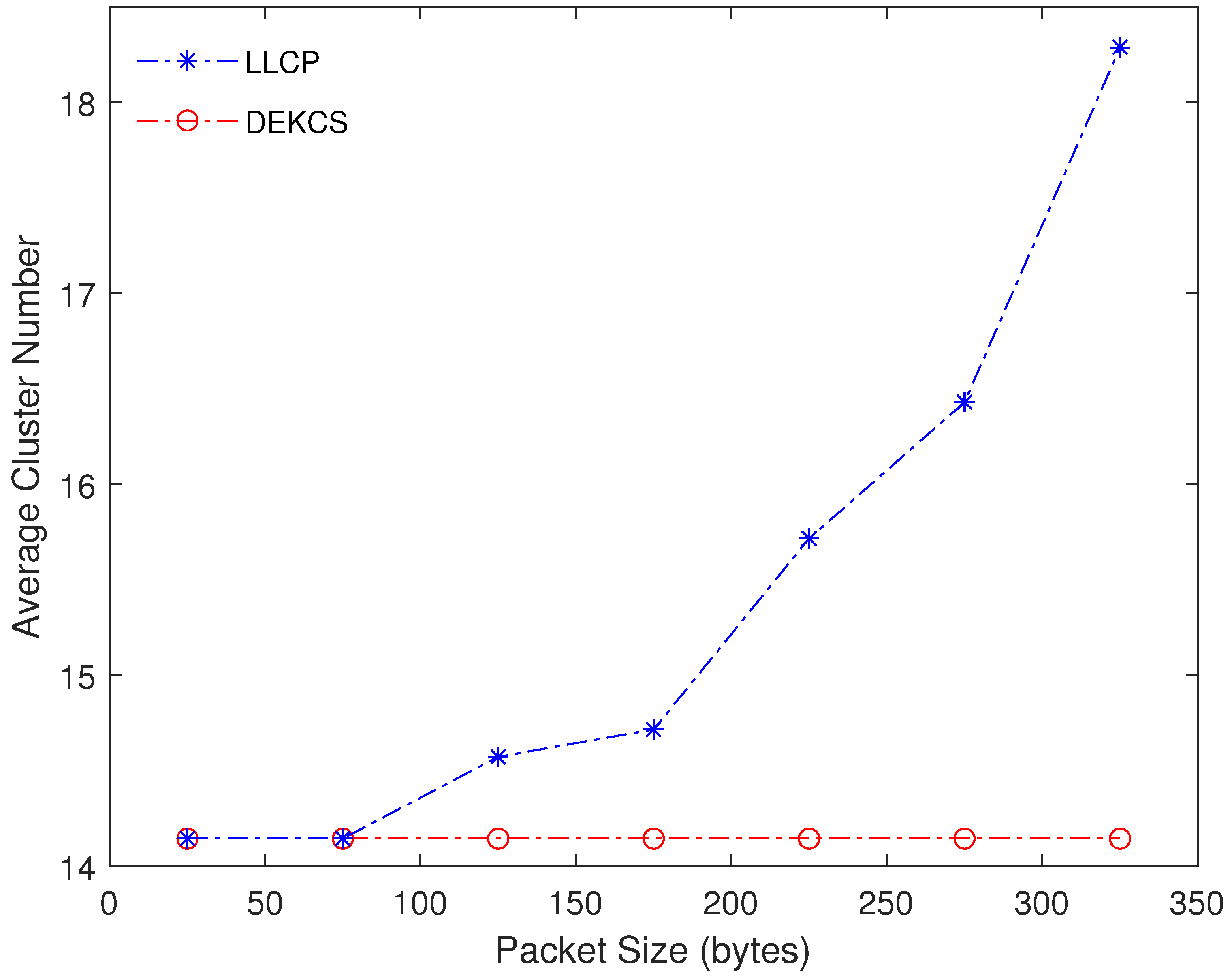
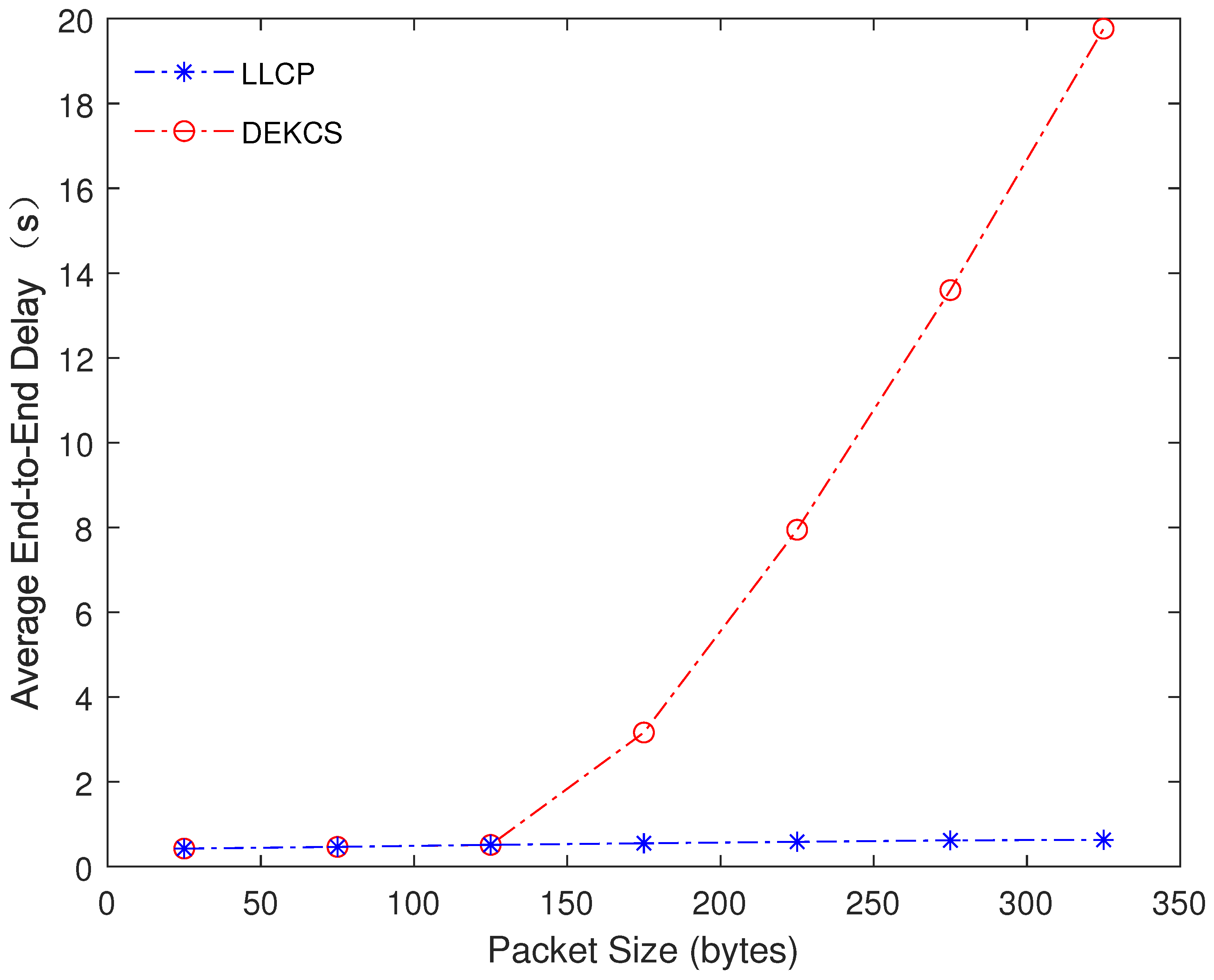
4.2. Performance under Different Packet Sizes
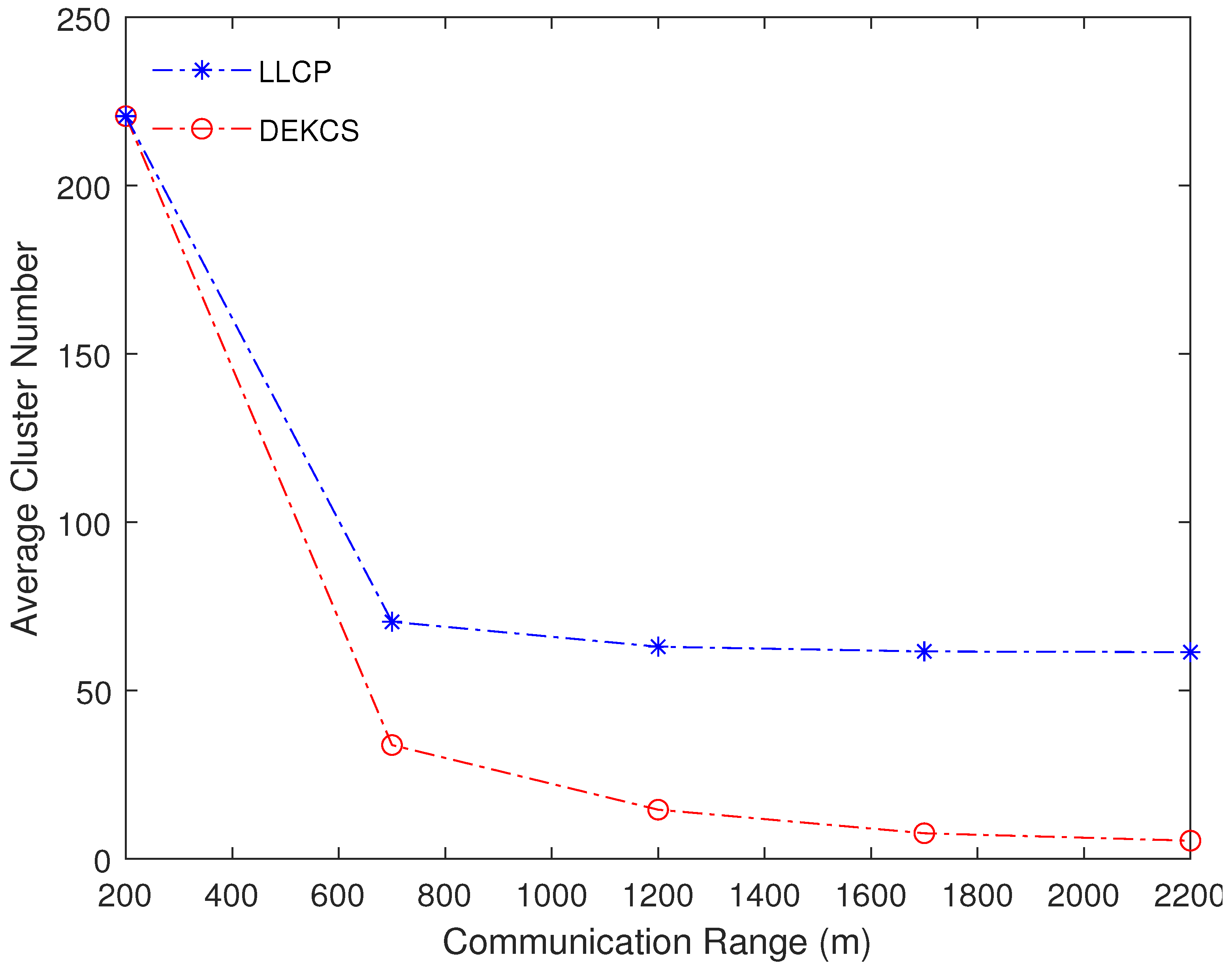
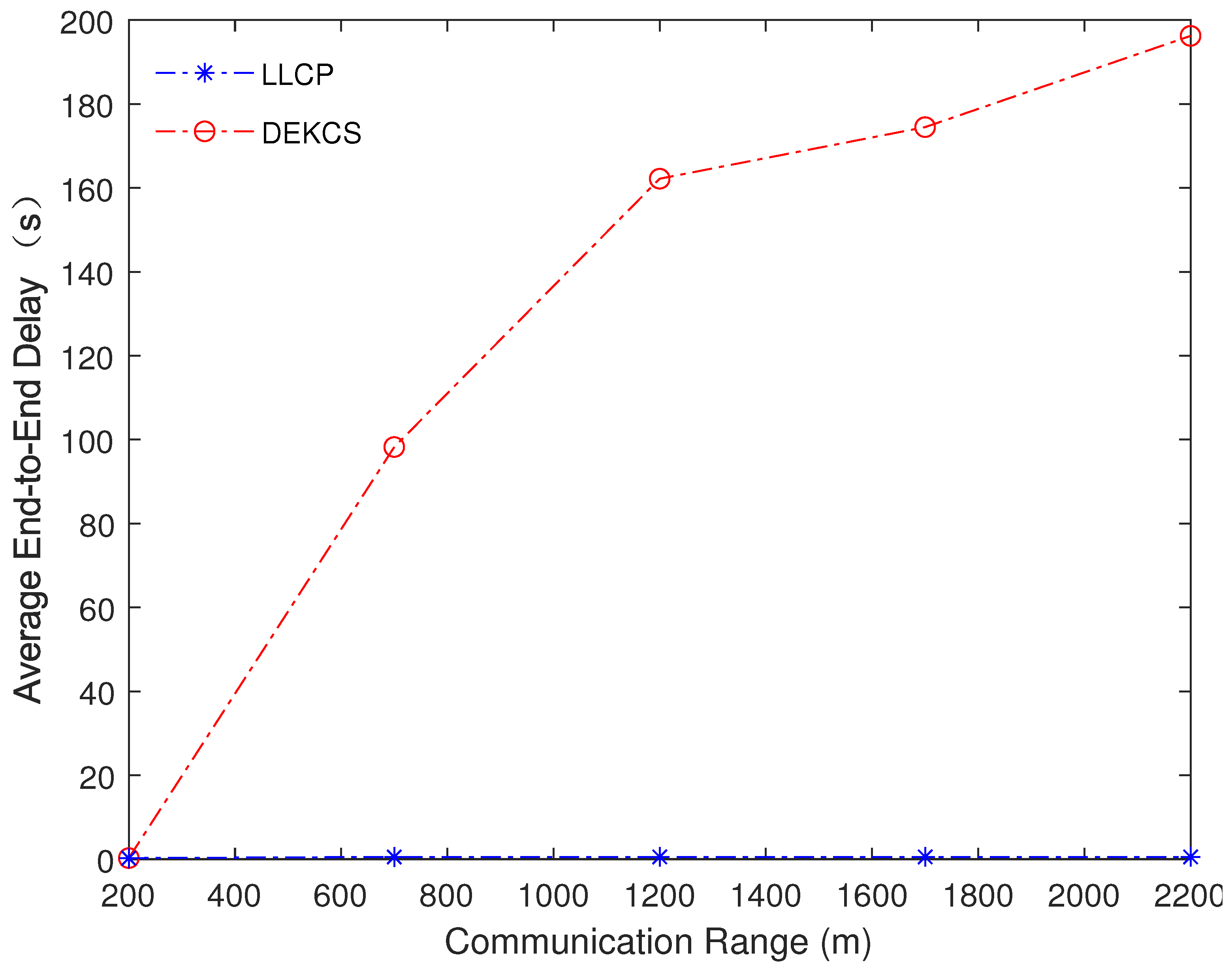
4.3. Performance under Different Communication Ranges
5. Conclusions
Author Contributions
Funding
Institutional Review Board Statement
Informed Consent Statement
Data Availability Statement
Conflicts of Interest
Abbreviations
| UASNs | underwater acoustic sensor networks |
| LLCP | node load and location-based clustering protocol for UASNs |
| DEKCS | distance and energy-constrained k-means clustering scheme |
| LEACH | low-energy adaptive clustering hierarchy |
| ACUN | adaptive clustering routing algorithm for underwater wireless sensor networks |
| ANCRP | anchor nodes assisted cluster-based routing protocol |
| GTC | game-theory-based clustering scheme |
| UCPSO | unequal clustering method based on particle swarm optimization |
| DNC-MPRP | distributed node clustering routing protocol with mobility pattern support |
| EOCSR | energy hole mitigation through optimized cluster head selection and strategic routing |
| CCCS | centralized control-based clustering scheme |
| EULC | energy-balanced unequal layering clustering |
| EEUCP | energy efficient underwater wireless sensor networks clustering protocol |
| MCBOR | energy-aware multilayer clustering-based butterfly optimization routing |
| EAMC | energy-aware multilevel clustering scheme |
| FNCBR | floating nodes assisted cluster-based routing |
| NS-3 | Network Simulator 3 |
References
- Coutinho, R.W.L.; Boukerche, A. OMUS: Efficient Opportunistic Routing in Multi-Modal Underwater Sensor Networks. IEEE Trans. Wirel. Commun. 2021, 20, 5642–5655. [Google Scholar] [CrossRef]
- Hao, K.; Ding, Y.; Li, C.; Wang, B.; Liu, Y.; Du, X.; Wang, C.Q. An Energy-Efficient Routing Void Repair Method Based on an Autonomous Underwater Vehicle for UWSNs. IEEE Sens. J. 2021, 21, 5502–5511. [Google Scholar] [CrossRef]
- Shen, Z.; Yin, H.; Xing, F.; Ji, X.; Huang, A. A distributed routing-aware power control scheme for underwater wireless sensor networks. Comput. Commun. 2023, 210, 10–21. [Google Scholar] [CrossRef]
- Wang, Q.; Li, J.; Qi, Q.; Zhou, P.; Wu, D.O. An Adaptive-Location-Based Routing Protocol for 3-D Underwater Acoustic Sensor Networks. IEEE Internet Things J. 2021, 8, 6853–6864. [Google Scholar] [CrossRef]
- Shen, Z.; Yin, H.; Jing, L.; Liang, Y.; Wang, J. A Cooperative Routing Protocol Based on Q-Learning for Underwater Optical-Acoustic Hybrid Wireless Sensor Networks. IEEE Sens. J. 2022, 22, 1041–1050. [Google Scholar] [CrossRef]
- Zenia, N.Z.; Kaiser, M.S.; Mahmud, M.; Ahmed, M.R.; Kaiwartya, O.; Kamruzzaman, J. REER-H: A Reliable Energy Efficient Routing Protocol for Maritime Intelligent Transportation Systems. IEEE Trans. Intell. Transp. Syst. 2023, 24, 13654–13669. [Google Scholar] [CrossRef]
- Yang, G.; Guo, Q.; Ding, H.; Yan, Q.; Huang, D.D. Joint Message-Passing-Based Bidirectional Channel Estimation and Equalization With Superimposed Training for Underwater Acoustic Communications. IEEE J. Ocean. Eng. 2021, 46, 1463–1476. [Google Scholar] [CrossRef]
- Mei, H.; Wang, H.; Shen, X.; Jiang, Z.; Bai, W.; Wang, C.; Zhang, Q. An Adaptive Routing Protocol for Underwater Acoustic Sensor Networks With Ocean Current. IEEE Sens. J. 2023, 23, 28220–28243. [Google Scholar] [CrossRef]
- Jha, A.V.; Appasani, B.; Khan, M.S.; Song, H.H. A Novel Clustering Protocol for Network Lifetime Maximization in Underwater Wireless Sensor Networks. IEEE Trans. Green Commun. Netw. 2024. [Google Scholar] [CrossRef]
- He, S.; Li, Q.; Khishe, M.; Salih Mohammed, A.; Mohammadi, H.; Mohammadi, M. The optimization of nodes clustering and multi-hop routing protocol using hierarchical chimp optimization for sustainable energy efficient underwater wireless sensor networks. Wirel. Netw. 2024, 30, 233–252. [Google Scholar] [CrossRef]
- Omeke, K.G.; Mollel, M.S.; Ozturk, M.; Ansari, S.; Zhang, L.; Abbasi, Q.H.; Imran, M.A. DEKCS: A Dynamic Clustering Protocol to Prolong Underwater Sensor Networks. IEEE Sens. J. 2021, 21, 9457–9464. [Google Scholar] [CrossRef]
- Heinzelman, W.B.; Chandrakasan, A.P.; Balakrishnan, H. An application-specific protocol architecture for wireless microsensor networks. IEEE Trans. Wirel. Commun. 2002, 1, 660–670. [Google Scholar] [CrossRef]
- Sathish, K.; Venkata, R.C.; Anbazhagan, R.; Pau, G. Review of Localization and Clustering in USV and AUV for Underwater Wireless Sensor Networks. Telecom 2023, 4, 43–64. [Google Scholar] [CrossRef]
- Zhang, Q.; Wang, H.; Zhao, R.; Shen, X.; He, K.; Zhang, H. The Design of Clustering Algorithm and MAC Protocol for Low Delay Underwater Acoustic Sensor Networks. IEEE Sens. J. 2023, 23, 3251–3261. [Google Scholar] [CrossRef]
- Datta, A.; Dasgupta, M. Energy Efficient Layered Cluster Head Rotation Based Routing Protocol for Underwater Wireless Sensor Networks. Wirel. Pers. Commun. 2022, 125, 2497–2514. [Google Scholar] [CrossRef]
- Goyal, N.; Kumar, A.; Popli, R.; Awasthi, L.K.; Sharma, N.; Sharma, G. Priority based data gathering using multiple mobile sinks in cluster based UWSNs for oil pipeline leakage detection. Clust. Comput. 2022, 25, 1341–1354. [Google Scholar] [CrossRef]
- Yang, Y.; Wu, Y.; Yuan, H.; Khishe, M.; Mohammadi, M. Nodes clustering and multi-hop routing protocol optimization using hybrid chimp optimization and hunger games search algorithms for sustainable energy efficient underwater wireless sensor networks. Sustain. Comput. Inform. Syst. 2022, 35, 100731. [Google Scholar] [CrossRef]
- Ayaz, M.; Ammad-Uddin, M.; Sharif, Z.; Hijji, M.; Mansour, A. A hybrid data collection scheme to achieve load balancing for underwater sensor networks. J. King Saud Univ. Comput. Inf. Sci. 2023, 35, 74–86. [Google Scholar] [CrossRef]
- Kaur, P.; Kaur, K.; Singh, K.; Bharany, S.; Almazyad, A.S.; Xiong, G.; Mohamed, A.W.; Shokouhifar, M.; Werner, F. Acoustic Monitoring in Underwater Wireless Sensor Networks Using Energy-Efficient Artificial Fish Swarm-Based Clustering Protocol (EAFSCP). Preprints 2023, 2023101325. [Google Scholar] [CrossRef]
- Kaveripakam, S.; Chinthaginjala, R. Energy balanced reliable and effective clustering for underwater wireless sensor networks. Alex. Eng. J. 2023, 77, 41–62. [Google Scholar] [CrossRef]
- Yang, Q.; Chen, Y.; Dong, W.; Li, T.; Zhu, R.; Huang, X. Cluster-Based Spatial–Temporal MAC Scheduling Protocol for Underwater Sensor Networks. IEEE Sens. J. 2023, 23, 17690–17702. [Google Scholar] [CrossRef]
- Wan, Z.; Liu, S.; Ni, W.; Xu, Z. An energy-efficient multi-level adaptive clustering routing algorithm for underwater wireless sensor networks. Clust. Comput. 2019, 22, 14651–14660. [Google Scholar] [CrossRef]
- Karim, S.; Shaikh, F.K.; Aurangzeb, K.; Chowdhry, B.S.; Alhussein, M. Anchor Nodes Assisted Cluster-Based Routing Protocol for Reliable Data Transfer in Underwater Wireless Sensor Networks. IEEE Access 2021, 9, 36730–36747. [Google Scholar] [CrossRef]
- Xing, G.; Chen, Y.; Hou, R.; Dong, M.; Zeng, D.; Luo, J.; Ma, M. Game-Theory-Based Clustering Scheme for Energy Balancing in Underwater Acoustic Sensor Networks. IEEE Internet Things J. 2021, 8, 9005–9013. [Google Scholar] [CrossRef]
- Hou, R.; Fu, J.; Dong, M.; Ota, K.; Zeng, D. An Unequal Clustering Method Based on Particle Swarm Optimization in Underwater Acoustic Sensor Networks. IEEE Internet Things J. 2022, 9, 25027–25036. [Google Scholar] [CrossRef]
- Chenthil, T.R.; Jesu Jayarin, P. An energy-efficient distributed node clustering routing protocol with mobility pattern support for underwater wireless sensor networks. Wirel. Netw. 2022, 28, 3367–3390. [Google Scholar] [CrossRef]
- Gupta, S.; Singh, N.P. Energy hole mitigation through optimized cluster head selection and strategic routing in Internet of Underwater Things. Int. J. Commun. Syst. 2022, 35, e5283. [Google Scholar] [CrossRef]
- Tian, W.; Zhao, Y.; Hou, R.; Dong, M.; Ota, K.; Zeng, D.; Zhang, J. A Centralized Control-Based Clustering Scheme for Energy Efficiency in Underwater Acoustic Sensor Networks. IEEE Trans. Green Commun. Netw. 2023, 7, 668–679. [Google Scholar] [CrossRef]
- Hou, R.; He, L.; Hu, S.; Luo, J. Energy-Balanced Unequal Layering Clustering in Underwater Acoustic Sensor Networks. IEEE Access 2018, 6, 39685–39691. [Google Scholar] [CrossRef]
- Bhaskarwar, R.V.; Pete, D.J. Energy efficient clustering with compressive sensing for underwater wireless sensor networks. Peer-to-Peer Netw. Appl. 2022, 15, 2289–2306. [Google Scholar] [CrossRef]
- Chenthil, T.R.; Jesu Jayarin, P. An Energy-Aware Multilayer Clustering-Based Butterfly Optimization Routing for Underwater Wireless Sensor Networks. Wirel. Pers. Commun. 2022, 122, 3105–3125. [Google Scholar] [CrossRef]
- Chinnasamy, S.; Naveen, J.; Alphonse, P.J.A.; Dhasarathan, C.; Sambasivam, G. Energy-Aware Multilevel Clustering Scheme for Underwater Wireless Sensor Networks. IEEE Access 2022, 10, 55868–55875. [Google Scholar] [CrossRef]
- Jatoi, G.M.; Das, B.; Karim, S.; Pabani, J.K.; Krichen, M.; Alroobaea, R.; Kumar, M. Floating Nodes Assisted Cluster-Based Routing for Efficient Data Collection in Underwater Acoustic Sensor Networks. Comput. Commun. 2022, 195, 137–147. [Google Scholar] [CrossRef]
- Song, S.; Liu, J.; Guo, J.; Zhang, C.; Yang, T.; Cui, J. Efficient Velocity Estimation and Location Prediction in Underwater Acoustic Sensor Networks. IEEE Internet Things J. 2022, 9, 2984–2998. [Google Scholar] [CrossRef]


| Parameter | Description |
|---|---|
| The upper limit of intra-cluster information transmission capacity | |
| The max channel utilization of the cluster head | |
| R | The communication rate of the physical layer |
| The duration of one time frame for the cluster head | |
| The minimum idle time of the cluster head within one time frame | |
| The time slot scheduling moment of cluster member i in time frame M | |
| The time slot length of cluster member i in time frame M | |
| The propagation delay from cluster member i to the cluster head | |
| The channel utilization of the cluster head in the Mth time frame | |
| The idle waiting time of the cluster head caused by cluster member i in the Mth time frame | |
| The guard interval | |
| A gap between the arrival time of the first data packet from the next time frame at the cluster head and the arrival time of the last cluster member’s data packet from the previous time frame | |
| The number of cluster members | |
| The maximum number of cluster members | |
| The time slot length of the cluster head in the time frame M | |
| The node number to be removed | |
| The total node number within the cluster | |
| The node degree | |
| The number of neighboring node | |
| The cluster cohesion | |
| The distance between cluster member i and the cluster head | |
| The neighbor node set | |
| The neighbor node set of neighbor node i | |
| The node locations | |
| The minimum neighbor node number | |
| The maximum distance | |
| The node farthest from the cluster head | |
| The maximum number of cluster members when clustering with node i and its neighboring nodes | |
| The node with the minimum node degree | |
| The adjusted neighbor node set | |
| The node type of node i | |
| The clustering priority | |
| The neighbor node set of neighbor node i | |
| The experimental average end-to-end delay | |
| The experimental average cluster number | |
| The total number of independent replication simulation | |
| The end-to-end delay of the jth data packet in the ith independent replication simulation | |
| The total number of successfully received data packets in the ith independent replication simulation | |
| The cluster number in the ith independent replication simulation |
| Parameter | Description |
|---|---|
| Src | Source node address |
| Dest | Destination node address |
| Type | Packet type |
| CM | Address of cluster member |
| TS | Time slot scheduling of sensor node |
| CF Packet | Cluster formation packet |
| Slot | Time slot of cluster member |
| Slot | Time slot of cluster header |
| Idle | Idle waiting time |
| CF Phase | Cluster formation phase |
| Parameter | Values |
|---|---|
| Sensor node number | 50–500 |
| Packet size | 25–325 bytes |
| Node location | Random deployment |
| Number of independent replication simulation | 5 |
| Communication range | 200–2200 m |
Disclaimer/Publisher’s Note: The statements, opinions and data contained in all publications are solely those of the individual author(s) and contributor(s) and not of MDPI and/or the editor(s). MDPI and/or the editor(s) disclaim responsibility for any injury to people or property resulting from any ideas, methods, instructions or products referred to in the content. |
© 2024 by the authors. Licensee MDPI, Basel, Switzerland. This article is an open access article distributed under the terms and conditions of the Creative Commons Attribution (CC BY) license (https://creativecommons.org/licenses/by/4.0/).
Share and Cite
Mei, H.; Wang, H.; Shen, X.; Jiang, Z.; Yan, Y.; Sun, L.; Xie, W. Node Load and Location-Based Clustering Protocol for Underwater Acoustic Sensor Networks. J. Mar. Sci. Eng. 2024, 12, 982. https://doi.org/10.3390/jmse12060982
Mei H, Wang H, Shen X, Jiang Z, Yan Y, Sun L, Xie W. Node Load and Location-Based Clustering Protocol for Underwater Acoustic Sensor Networks. Journal of Marine Science and Engineering. 2024; 12(6):982. https://doi.org/10.3390/jmse12060982
Chicago/Turabian StyleMei, Haodi, Haiyan Wang, Xiaohong Shen, Zhe Jiang, Yongsheng Yan, Lin Sun, and Weiliang Xie. 2024. "Node Load and Location-Based Clustering Protocol for Underwater Acoustic Sensor Networks" Journal of Marine Science and Engineering 12, no. 6: 982. https://doi.org/10.3390/jmse12060982
APA StyleMei, H., Wang, H., Shen, X., Jiang, Z., Yan, Y., Sun, L., & Xie, W. (2024). Node Load and Location-Based Clustering Protocol for Underwater Acoustic Sensor Networks. Journal of Marine Science and Engineering, 12(6), 982. https://doi.org/10.3390/jmse12060982