Abstract
The continuous improvement in the seaworthiness of Arctic shipping routes has caused an urgent international demand for meteorological and sea ice information. In view of the diversity of Arctic meteorological and sea ice information websites and the uneven service levels of the websites, and to assist Arctic navigation ships in selecting timely, stable, and reliable meteorological and sea ice information, this paper summarizes the websites providing Arctic meteorological and sea ice information. Constructing an evaluation indicator system for the service level of the Arctic meteorological and sea ice information websites from the two dimensions of data quality and browsing experience, this system integrates the cloud model, the Dempster–Shafer (D-S) evidence theory, and the Technique for Order of Preference by Similarity to Ideal Solution (TOPSIS) method to construct a corresponding service-level evaluation and decision optimization process of Arctic meteorological and sea ice information websites. Finally, through case analysis, the feasibility of this research method is demonstrated.
1. Introduction
Compared with traditional shipping routes, the opening of Arctic shipping routes has greatly shortened the distance from Asia or North America to Europe and brought great benefits to the shipping industry. The extent of sea ice in the Arctic has been shrinking since 1970, and predictive studies indicate that there will be an “ice-free summer”, making Arctic shipping routes an increasingly important shipping strategy [1]. Obtaining timely and accurate information on the navigational environment in the Arctic region can assist ships in making the correct decision and reduce the navigational risk to a certain extent. In addition, the International Maritime Organization (IMO) has implemented an e-navigation strategy to exchange maritime information electronically between the ship end and shore end [2]. Therefore, accurate and timely polar navigation information is of great significance.
Paying attention to the environmental variables involved in research related to Arctic navigation safety, Sahin and Kum [3] used the improved fuzzy analytic hierarchy process to summarize various navigational risk factors in the Arctic region, including harsh environmental conditions and lack of hydrometeorological information. Zhang et al. (2020) constructed a real-time assessment and prediction model for the maritime risk state of Arctic shipping routes by categorizing the factors affecting navigation in the Arctic region into solid and dynamic factors (such as sea temperature, wind, and sea ice concentration) [4]. To determine an economically safe shipping route in the Arctic Ocean, Lee et al. (2021) combined sea ice concentration, sea ice thickness, sea ice type, wind, wave, ocean current and other risk factors to conduct risk assessments of navigation conditions [5]. Based on the improved polar operational limit assessment risk indexing system (POLARIS), Li et al. (2020) built a navigation plan model by comprehensively considering sea ice, waves, ocean currents, wind, and temperature [6]. Li et al. (2021) have constructed a risk assessment model for LNG carriers sailing in Arctic waters by using dynamic Bayesian networks and combining wind, sea temperature, wave and sea ice density data [7]. Based on the sea ice status data from 2011 to 2020, An et al. (2022) identified three key waters and navigation windows affecting the safety of navigation ships along the Northeast Passage [8]. Yang et al. (2024) comprehensively analyzed 149 relevant pieces of literature exploring the main risk factors and data sources considered by different risk assessment models [9]. Considering the variables involved in the above research, the variables concerned in this paper are divided into two categories: sea ice information and meteorological information. Sea ice information includes sea ice concentration, sea ice thickness and sea ice type. Meteorological information includes wind, sea temperature, waves, and ocean currents.
Reviewing the relevant research on Arctic navigation safety and noting the website sources of relevant research environmental data, Kotovirta et al. (2009) built an ice route navigation optimization system based on the sea ice information provided by the Swedish Meteorological and Hydrological Institute [10]. Nam et al. (2013) used information on sea ice, sea temperature, wind, and waves to construct a navigation model to determine the best Arctic shipping routes, with data from the European Centre for Medium-Range Weather Forecasts (ECMWF) [11]. Liu et al. (2016) designed an autonomous ice navigation system using the sea ice information of the Canadian Ice Service [12]. Knol et al. (2018) analyzed the service types and service objects of three websites, namely BarentsWatch, Polar View and Arctic Web [13]. Zhang et al. (2019) built a data-driven model using sea ice, wind, wave, sea temperature and other data from the National Marine Environmental Forecasting Center to predict the energy efficiency of Arctic ships [14]. Li et al. (2020) comprehensively considered sea ice, waves, ocean currents, wind and temperature, and conducted a path optimization study considering fuel consumption. The data came from the UK Met Office [6]. Wu et al. (2022) used the data of the National Snow and Ice Data Center (NSIDC) to build a ship navigation information service system [15]. Chen et al. (2023) used the sea ice concentration and sea ice thickness data products provided by the Copernicus Marine Environment Monitoring Service (CMEMS) to achieve multi-objective route optimization of the Arctic route [16]. Inoue (2021) introduced the predictable nature of Arctic weather and sea ice and mentioned the ECMWF data [17]. The above representative data sources are evaluated in Section 2.1.
Many scholars have conducted research on website evaluation. Li et al. (2011) conducted an evaluation of Chinese e-commerce websites in terms of content, ease of use, offers, and emotional factors [18]. Li et al. (2020) combined a gray fuzzy comprehensive analysis and entropy weight Technique for Order of Preference by Similarity to Ideal Solution (TOPSIS) method to explore the factors of successful website design from the aspects of information quality, website design, service quality, security and privacy [19]. However, the service level evaluation and decision-making optimization problem of the Arctic meteorological and sea ice information websites has the characteristics of fuzziness, randomness and uncertainty. Cloud models can complete the conversion between qualitative and quantitative information and effectively solve the problems of fuzziness and randomness in evaluation problems [20]. The Dempster–Shafer (D-S) evidence theory can integrate multi-dimensional information membership based on its strong information synthesis ability, thus effectively solving the uncertainty of evaluation problems [21]. Then, the TOPSIS method can be used to make optimal decisions for different alternatives with the same evaluation level [22], thus realizing an evaluation of the service level of the Arctic meteorological and sea ice information websites and optimal decision-making.
Since Arctic meteorological and sea ice information is relatively limited and scattered among different sources, this paper will collect and summarize open-source information websites and website information status. In view of the diversity of Arctic meteorological and sea ice information websites, the uneven service levels of websites, and to assist ships in selecting timely, stable and reliable information, this paper integrates a cloud model, the D-S evidence theory and the TOPSIS method to construct a service level evaluation and optimization process suitable for Arctic meteorological and sea ice information websites to assist ships in making correct decisions and reduce navigation risks.
2. Construction of the Indicator System
2.1. Research Objects
The International Code for Ships Operating in Polar Waters (Polar Code) and Guidance on Arctic Navigation in the Northeast Route clearly point out that the bridge of polar ships must obtain the latest weather and sea ice information to be able to know the developing weather and sea ice trends [23,24]. However, sea ice and meteorological environment conditions in the Arctic are complex and changeable, resulting in relatively limited meteorological and sea ice information in the region. These data are distributed among various databases and websites. Therefore, Arctic meteorological information websites and sea ice information websites were used as research objects, and the main information sources were collected and summarized. Meteorological information mainly includes wind, sea temperature, ocean currents and waves. Sea ice information includes sea ice concentration, sea ice thickness and sea ice type. Table 1 and Table 2 show detailed information from meteorological and sea ice websites indicating time resolution, spatial resolution, time range, data presentation form and acquisition method provided by each website.

Table 1.
Meteorological information.
Table 2.
Sea ice information.
2.2. Construction of Evaluation Indicator System
Based on relevant research and the characteristics of Arctic meteorological and sea ice information, this paper presents an evaluation system for the service level of Arctic meteorological and sea ice information websites from both quantitative and qualitative aspects, as shown in Figure 1.
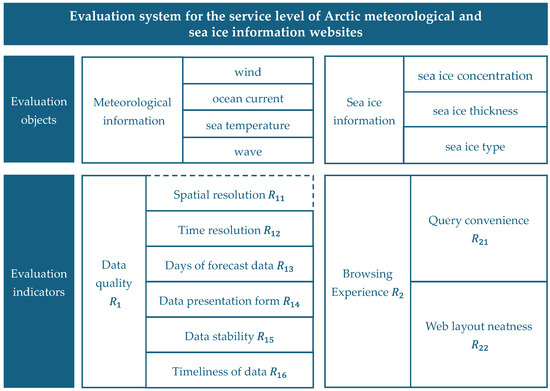
Figure 1.
Evaluation system for the service level of Arctic meteorological and sea ice information websites.
This system includes two primary indicators and eight secondary indicators:
(1) Data quality ()
Spatial resolution () refers to the measure of the smallest discernible detail in an image or data.
Time resolution () is the time frequency of data image publication, that is, how often the website publishes information.
Days of forecast data () refers to the time range of future conditions provided in the meteorological and sea ice information.
Data presentation form () mainly includes image, numerical data, text data and other forms.
Data stability () is the stability of the time frequency of data release in the range of one month, that is, whether the website publishes information in accordance with the provided time resolution law, as shown in Equation (1).
where represents the monthly stability rate of data; indicates the number of days in a month when the data are unstable; represents the total number of days in the research month. This paper takes May 2023 data as an example, and .
Timeliness of data () refers to whether the published data reflect the latest information, expressed by the number of days between the date on which the information is available and the date on which the information is published.
(2) Browsing experience ()
Query convenience () refers to the degree to which the user can easily and quickly access the required information in the process of information retrieval.
Web layout neatness () refers to the organization and presentation of layout, font, color and other elements in web design, so that the web content is clear, beautiful and easy to read.
In meteorological information, information on the variables is generally provided in the form of pictures, charts or dynamic interactive maps. It is difficult to know their spatial resolution, therefore, the spatial resolution indicator is not considered in the evaluation of meteorological information websites.
3. Model and Methods
3.1. Evaluated Websites
To achieve the evaluation and optimization of Arctic meteorological and sea ice information websites under different service levels, this paper constructs a set of evaluation and optimization processes suitable for these websites, as shown in Figure 2.
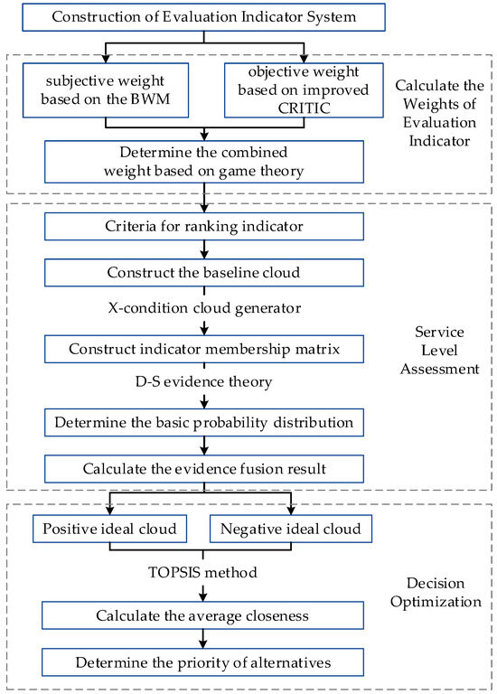
Figure 2.
Flow chart of assessment and decision-making optimization.
Firstly, the subjective and objective weights of indicators are calculated by the Best-Worst Method (BWM) and improved CRiteria Importance Through Intercriteria Correlation (CRITIC) method, respectively, and the combined weight of each indicator is obtained by game theory. Secondly, the base cloud is constructed according to the grade evaluation criteria of the indicators, the membership degree of each indicator is calculated using the X-condition cloud generator, and then converted into the basic probability distribution through the D-S evidence theory for evidence fusion. Finally, the optimal order of the final decision is determined by the average closeness value according to the TOPSIS method.
3.2. Calculate the Weights of Evaluation Indicator
3.2.1. Obtaining Subjective Weight Based on the BWM
According to the importance of the best indicator and the worst indicator relative to other indexes, two comparison vectors and are determined respectively [25]. Then, the following calculation formula is used to calculate the subjective weight of each indicator.
where is absolute error, and the optimization goal is to minimize it, represents the weight of the best indicator, is the best weight of the indicator , represents the ratio of the importance of the best indicator to that of the indicator , represents the weight of the worst indicator, and represents the ratio of importance of the indicator to the worst indicator .
3.2.2. Obtaining Objective Weight Based on Improved CRITIC
The CRITIC method is an objective weight assignment method proposed by Diakoulaki et al. [26]. Its basic idea is to comprehensively measure the objective weight of each indicator by the contrast intensity and conflict between the evaluation indicators. First, we describe a decision matrix and find the normalization of the decision matrix, as shown in Equations (3) and (4).
where represents data after standardized processing, represents the original data value of the indicators, represents the maximum value of indicator , and represents the minimum value of indicator .
Based on the improved CRITIC method [27], the objective weight of each indicator is calculated by the level of contrast, the degree of conflict, and the amount of data between each indicator, as shown in Equation (5).
where represents the amount of data, is the objective weight of indicator .
3.2.3. Obtaining Combined Weight Based on Game Theory
Combining the weights obtained by using the BWM method and the improved CRITIC, obtain the combined weights, as shown in Equation (6).
Using the game theory [28], the weight matrix is optimized by linear combination to obtain the minimum optimization value, as shown in Equation (7).
The above formula is calculated to determine the final combined weight, as shown in Equation (8).
where is the combined weight calculated by game theory, represents weight coefficient and , and represents single weight matrix.
3.3. Service Level Assessment
3.3.1. Construct the Base Cloud Based on Cloud Model
The golden section search method and interval constraint method were used to calculate the basic data characteristics of qualitative and quantitative indicators, respectively, and the base cloud for evaluating the service level of Arctic meteorological and sea ice information websites was constructed. Based on relevant literature analysis and expert opinion consultation, the Arctic meteorological and sea ice information website service levels were divided into five grades: Excellent [8.0, 10.0], Very Good [6.0, 8.0), Good [4.0, 6.0), Fair [2.0, 4.0), and Poor [0.0, 2.0). All five levels were represented by cloud digital characteristics.
For the qualitative index, the golden section method was used to calculate standard cloud digital features and the efficient domain was [0, 10]; the quantitative index was conducted by the interval division method. Each generated five clouds, which are , , , , .
The calculation formulae of qualitative indicators are as follows:
The calculation formula of quantitative indicators is as shown in Equation (12).
where indicates a base cloud with the “Poor” rating, , respectively, represent the expectation value, entropy and hyperentropy of the base cloud at this evaluation level; indicates a base cloud with the “Fair” rating, , respectively, represent the expectation value, entropy and hyperentropy of the base cloud at this evaluation level; indicates a base cloud with the “Good” rating, , respectively, represent the expectation value, entropy and hyperentropy of the base cloud at this evaluation level; indicates a base cloud with the “Very Good” rating, , respectively, represent the expectation value; and indicates a base cloud with the “Excellent” rating, , respectively, represent the expectation value. , respectively, represent the upper and lower limits of the evaluation interval, belong to the boundary values of the adjacent service level evaluation interval, and have the same membership degree of 0.5 for the adjacent service levels.
3.3.2. Calculating the Degree of Membership Based on the Conditional Cloud Generator
A cloud generator is an algorithm for generating cloud models. Different output results and cloud images can be obtained by inputting different initial parameters [29]. The evaluation indicator system of Arctic meteorological and sea ice information website service levels includes qualitative and quantitative indicators. Therefore, this paper selects the X-condition cloud generator to complete the calculation of the indicator membership degree, and the algorithm is implemented as follows:
Input three numerical eigenvalues (), cloud drop number () and known quantitative values ().
Numerical calculation output:
where represents the membership degree of a quantitative number belonging to a qualitative concept , represents the expectation value, and represents random numbers generated by the cloud generator.
Output the degree of membership of a qualitative concept.
3.3.3. Evidence Synthesis Based on the D-S Evidence Theory
Transform each element in the membership matrix into a function that conforms to the evidence theory . Assuming that are basic probability distribution functions on the same identification framework, a combination rule of mass functions can be defined as follows:
where , representing the degree of conflict between the evidence.
3.4. Decision Optimization Based on the TOPSIS Method
The average closeness value between the alternatives and the two ideal clouds is calculated. A larger difference indicates the alternatives are closer to the ideal options, and the scheme corresponding to the maximum average of the two is generally taken as the best scheme for comprehensive decision-making [22].
where , respectively, represent the average closeness value difference between alternative options and the positive and negative ideal clouds.
4. Example Demonstration
Ten open-source websites that provide Arctic meteorological information and ten open-source websites that provide sea ice information were selected. Qualitative indicators include data presentation form, query convenience, and web layout neatness. Expert scoring within the range of [0, 10] was employed to obtain the original data. Quantitative indices included spatial resolution, time resolution, days of forecast data, data stability, and timeliness of data. The original data status of meteorological and sea ice information can be found in Table 3 and Table 4.
Table 3.
Original data of meteorological information.
Table 4.
Original data of sea ice information.
4.1. Determine the Weights of Evaluation Indicators
First, authoritative experts in the research field were invited to determine the best and worst indicators in the evaluation indicators, in which the best indicator () is the time resolution (), and the worst indicator () is the query convenience (). Then, experts scored the importance of the best and worst indicators relative to other indicators, and acquired two comparative vectors of meteorological information: = (1, 2, 3, 5, 4, 6, 7), = (7, 6, 4, 3, 5, 2, 1)T. Two comparative vectors of sea ice information were also acquired: = {2, 1, 4, 3, 6, 5, 7, 8), = (8, 5, 4, 7, 3, 6, 2, 1)T. The subjective weight based on expert experience was calculated by the BWM method, and the objective weight of each indicator was calculated by using the improved CRITIC. Finally, the combined weight was calculated based on game theory. The results are shown in Table 5 and Table 6.
Table 5.
Weights of evaluation indicators (meteorological information).
Table 6.
Weights of evaluation indicators (sea ice information).
4.2. Evaluating the Service Level
(1) Constructing the baseline cloud
The grading interval division method was used to set the grading interval of each quantitative indicator, as shown in Table 7.
Table 7.
Classification criteria for quantitative indicators.
The cloud digital characteristic values of each evaluation indicator under five evaluation levels were calculated. For qualitative indicators, the effective domain is [0, 10], which means that is 0 and is 10. The golden section method was used to calculate the cloud digital characteristic values of qualitative indicators by Equations (9)–(11). The interval division method was used to obtain the cloud digital characteristic values of the quantitative data by substituting into Equation (12) based on the criteria for the ranking of quantitative indicators that have been classified. The hyperentropy of the qualitative and quantitative indicators in the cloud digital characteristic values was 1/10 of the entropy value. The digital characteristic values of the baseline cloud are shown in Table 8, and the corresponding baseline cloud image is shown in Figure 3 and Figure 4. The evaluation clouds of each level were intertwined in pairs on the interval and there was a certain uncertainty.
Table 8.
The digital characteristic values of the baseline cloud.
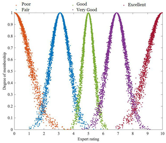
Figure 3.
Baseline cloud images of the qualitative indicators.
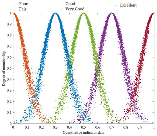
Figure 4.
Baseline cloud images of the quantitative indicators.
(2) Calculating the membership based on the conditional cloud generator
Membership degree was calculated according to the baseline cloud digital characteristic values (, , ) and quantified data of indicators () at different levels. For example, the cloud digital characteristic values of spatial resolution in the evaluation level of “Excellent” were (1, 0.085, 0.008) and the quantified data of University of Bremen (UOB) were = 0.995. Using the X-conditional cloud generator to generate 3000 random numbers and substituting them into Equation (14) yielded the membership degree of 0.998. The above calculations were performed sequentially thus forming the membership degree matrix. Due to space constraints, only the UOB is used here as an example, as shown in Table 9.
Table 9.
The membership degree of the cloud model for sea ice concentration information provided by the UOB ().
(3) Evidentialization of the membership degree
The membership degree obtained by the cloud model was converted into the basic probability distribution consistent with the definition of the evidence theory, for example, the basic probability distribution of the spatial resolution of the UOB in the evaluation grade “Excellent”: 0.998/(0.998 + 0.004 + 0.000 + 0.000 + 0.000) = 0.996. For the UOB, the basic probability distribution of sea ice concentration for the event {Excellent, Very Good, Good, Fair, Poor} is shown in Table 10.
Table 10.
Basic probability distribution of sea ice concentration of the UOB.
(4) Synthesizing the evidence
The basic probability distribution of each evaluation indicator was weighted first, and the event {Excellent, Very Good, Good, Fair, Poor} was synthesized by the evidence synthesis rule. Taking the calculation of sea ice concentration of the UOB in the evaluation grade “Excellent” as an example, after being weighted according to the weights assigned to each indicator, the resulting weighted evidence was (0.0019, 0, 0, 0, 0.0004) and seven pieces of evidence for each evaluation indicator were obtained. By substituting these values into a Formula (15), the membership degree of the UOB’s sea ice concentration fell within the “Excellent” evaluation grade with a degree of confidence at 0.977. According to the above calculation steps, the membership degree of each variable of the UOB could finally be obtained, as shown in Table 11. It can be seen in the table that the UOB had the best performance in terms of sea ice concentration information and the worst performance in terms of sea ice type information.
Table 11.
Grade probability of the variables of the UOB.
Similar to the previous calculation, the three variables from the UOB were further synthesized using the evidence synthesis rule. From the perspective of variables available on the website, it was considered that each variable had the same importance, that of one-third. Then, the weighted evidence could be obtained as (0.515, 0, 0, 0, 0.485), and three pieces of evidence from each variable could be determined. The membership degree of the UOB in the evaluation grade “Excellent” was 0.544 by substituting the above figures into Equation (15). The website service level evaluation of the UOB was ultimately determined based on the following probabilities: {Excellent, Very Good, Good, Fair, Poor}: {0.544, 0, 0, 0, 0.456}.
According to the above evaluation steps, other websites were evaluated and calculated in turn. The final service level evaluation probability of the meteorological and sea ice information websites is shown in Table 12 and Table 13, respectively. “Excellent” and “Poor” may coexist in the final evaluation results. It can be seen in Table 11 that the grade of sea ice type of the UOB was “Poor”, and the membership degree was 1. Influenced by the grade of sea ice type, the probabilities of “Excellent” and “Poor” in the final evaluation result of the UOB were closer after evidence fusion, but the evaluation grades of sea ice concentration and sea ice thickness were more satisfactory. The final evaluation result was “Excellent”.
Table 12.
Grade probability of service level of meteorological information websites.
Table 13.
Grade probability of service level of sea ice information websites.
In short, among the meteorological information websites, the evaluation grades of ECMWF and NMSRSS were {Excellent}, the evaluation grades of MT and NMEFC were {Very Good}, and the remaining were {Poor}. Among the sea ice information websites, the evaluation grades of UOB, CMEMS and MOOF were {Excellent} and the remaining were {Poor}.
4.3. Decision Optimization
Based on the TOPSIS method, different alternatives under the same evaluation level were further selected. First, the basic probability distribution of positive and negative ideal clouds was calculated in the same way as the above calculation method, as shown in Table 14.
Table 14.
The basic probability distribution of positive and negative ideal clouds.
According to Formulas (16) and (17), the closeness between each alternative and positive and negative ideal cloud was calculated. Taking the UOB as an example, the distance between the UOB and the positive ideal cloud was the absolute value of the difference between the membership degree of the evaluation grade of the UOB and the basic probability of the positive ideal cloud. This closeness was the difference between the mean maximum 0.4 and each website. That is, the corresponding difference between (0.544, 0, 0, 0, 0.456) and (1, 0, 0, 0, 0, 0) was taken as absolute value, and the result was (0.456, 0, 0, 0, 0.456). The mean value was obtained by (0.456 + 0 + 0 + 0 + 0.456)/5 = 0.182 and the closeness was obtained by 0.4 − 0.182 = 0.218. The closeness to the negative ideal cloud was the difference between each website and the mean minimum 0, which was 0.128 − 0 = 0.128. Taking the websites that provide sea ice information as examples, the calculation results are shown in Table 15 and Table 16.
Table 15.
The distance between each alternative and the positive ideal cloud.
Table 16.
The distance between each alternative and the negative ideal cloud.
Combined with the service level of each alternative, the average closeness between each alternative and positive and negative ideal cloud in meteorological and sea ice information was calculated respectively, as shown in Table 17 and Table 18.
Table 17.
The average closeness and difference between each alternative and positive and negative ideal cloud (meteorological information websites).
Table 18.
The average closeness and difference between each alternative and positive and negative ideal cloud (sea ice information websites).
According to the principle that the larger the difference in average closeness, the closer the alternatives are to the most desirable solution, these are shown in order of preference for each alternative in meteorological and sea ice information in Table 19.
Table 19.
Decision order of meteorological and sea ice information websites.
4.4. Analyzing the Results
Through the related research in this paper, the information website service level evaluation optimization sequence is obtained. In the meteorological information website evaluation indicators, time resolution is an important factor affecting service level. The time resolution of NMSRS is real time, ECMWF is three hours, and MT and NMEFC are six hours, all of which can meet the actual navigation needs. Most of these websites provide information on multiple variables in a more intuitive form, and the data stability and timeliness are also high, so the levels of information-comprehensive service are relatively high, and they can be used as a reference for obtaining meteorological information during navigation. For WNI, CMFE, GMW, AARI and CMEMS, from the perspective of the variables that the websites provided, these websites only provide single variable information. On the other hand, from the perspective of website information quality, although the grade of their data stability and presentation form are very close to the top several websites, their comprehensive service levels are greatly affected by their large time resolution.
In the sea ice information websites, CMEMS, MOOF, UOB and MP have a high information service level. First, from the perspective of the variables available on the websites, these websites can provide relatively comprehensive variable information. On the other hand, from the perspective of the information quality of the websites, the information of these websites is updated regularly, and the time resolution and spatial resolution are small, which can meet the different information needs of ships during navigation. As for NERSC, USNIC, CMFC, NSRIO, WNI and EUMETSAT, most of them can only provide a single variable of information with high temporal and spatial resolution, presenting a low comprehensive service level.
This study also conducted expert interviews with captains who possess actual Arctic sailing experience using the Delphi method. The interview results were generally consistent with the evaluation results of this paper. In terms of the acquisition of meteorological information, the captains prefer to use the information with smaller resolution and a more intuitive presentation form during the voyage. In this study of this paper, NMSRSS, ECMWF, MT and NMEFC all provided smaller spatial and temporal resolution and are presented in a more intuitive way, ranking a high comprehensive service level. In addition, the captains said that polar research ships have special characteristics in the course of sailing, thus the demand for meteorological information is generally limited and consulted every six hours.
In this study, NMSRSS, ECMWF, MT and NMEFC, which ranked highly in comprehensive service level, meet the actual navigation needs of ships and can be used as a reliable information reference during the actual navigation of ships. In terms of the acquisition of sea ice information, the UOB enjoys a high reputation in the field of sea ice research, and the release of information has high reliability and timeliness. Thus, the captains prefer to use the Intuitive Sea Ice Information Service (ISIS) provided by the UOB. According to this study, the CMEMS is significantly better than the UOB in terms of information service level. This is partly because the CMEMS provides more comprehensive data and analysis than the UOB, covering key sea ice indicators such as sea ice concentration, sea ice thickness and sea ice type. In addition, the CMEMS and the MOOF were respectively able to provide steady 7-day and 1-day forecast data. Therefore, the CMEMS, MOOF, UOB and MP can be used as a reference of acquisition of sea ice information for captains.
The website research and evaluations for this study were completed in October 2023, and the information published on the websites may have since been updated. This paper only provides a set of decision-making processes for the Arctic navigation information websites based on their actual situation and the evaluation results may have changed with the update of the websites. The website evaluation result is only a reference and does not represent the inevitable advantages and disadvantages of the websites. It is recommended that relevant decision makers should consider their own needs and various factors in combination with the evaluation results to make the most reasonable decisions.
4.5. Discussion
The above example shows that the evaluation and decision optimization process of Arctic meteorological and sea ice information websites is effective and feasible. Currently, there is little research on the Arctic meteorological and sea ice information services. Wu et al. (2022) have built a ship navigation information service system based on the meteorological and sea ice information that can be provided by a single website [15]. However, the evaluation of the service level of website data has not yet been achieved. In addition, although Knol et al. (2018) have analyzed different websites that can provide sea ice information in Arctic waters [13], they only include qualitative analyses of the websites. This paper constructs the evaluation indicator system for the service level of Arctic meteorological and sea ice information websites from both the quantitative aspect (website data quality) and the qualitative aspect (browsing experience). The evaluation and optimization of Arctic meteorological and sea ice information websites at different service levels were achieved.
Although some progress has been made, this study still has some limitations. In the evaluation of the websites, we only considered part of the information. Water depth is also an important factor affecting ship navigation. However, due to data scarcity, this variable was not considered in this paper. When water depth data are sufficient in the future, the proposed evaluation and optimization process can still be applied.
5. Conclusions
In the face of the uneven service levels of Arctic meteorological and sea ice information websites, considering the randomness, fuzziness and uncertainty of evaluation problems, a cloud model and the D-S evidence theory were used to evaluate the service level of Arctic meteorological and sea ice information websites. Based on the TOPSIS method for multi-attribute decision-making research, further decision optimization was achieved. Combined with the characteristics of Arctic meteorological and sea ice information, an evaluation indicator system for the service level of Arctic meteorological and sea ice information websites was designed from two dimensions: data quality and browsing experience. A set of decision optimization processes for Arctic navigation information websites was provided to realize the evaluation of the service level and decision optimization of Arctic meteorological and sea ice information websites, which provided a certain scientific basis for the selection of information during ship navigation.
Author Contributions
Conceptualization, T.-H.H.; data curation, Q.M.; writing—original draft, Q.M.; writing—review and editing, T.-H.H.; funding acquisition, B.H.; project administration, S.W.; supervision, W.L. All authors have read and agreed to the published version of the manuscript.
Funding
This research was funded by National Key Research and Development Program of China (Grant No. 2021YFC2801000), National Natural Science Foundation of China (Grant No. 52071199) and Shanghai Science and Technology Innovation Action Plan (Grant Nos. 22DZ1204503, 21DZ1205803).
Institutional Review Board Statement
Not applicable.
Informed Consent Statement
Not applicable.
Data Availability Statement
The data presented in this study are available from a public website.
Conflicts of Interest
Author Bing Han was employed by the company Shanghai Ship and Shipping Research Institute Co., Ltd. The remaining authors declare that the research was conducted in the absence of any commercial or financial relationships that could be construed as a potential conflict of interest.
References
- Liu, J.; Song, M.; Horton, R.M.; Hu, Y. Reducing Spread in Climate Model Projections of a September Ice-Free Arctic. Proc. Natl. Acad. Sci. USA 2013, 110, 12571–12576. [Google Scholar] [CrossRef] [PubMed]
- Korcz, K. Main Aspects of a Maritime E-Navigation Project. J. KONES 2019, 26, 83–90. [Google Scholar] [CrossRef][Green Version]
- Sahin, B.; Kum, S. Risk Assessment of Arctic Navigation by Using Improved Fuzzy-AHP Approach. Int. J. Marit. Eng. 2015, 157, 241. [Google Scholar] [CrossRef]
- Zhang, Y.; Hu, H.; Dai, L. Real-Time Assessment and Prediction on Maritime Risk State on the Arctic Route. Marit. Policy Manag. 2020, 47, 352–370. [Google Scholar] [CrossRef]
- Lee, H.-W.; Roh, M.-I.; Kim, K.-S. Ship Route Planning in Arctic Ocean Based on POLARIS. Ocean Eng. 2021, 234, 109297. [Google Scholar] [CrossRef]
- Li, Z.; Ringsberg, J.W.; Rita, F. A Voyage Planning Tool for Ships Sailing between Europe and Asia via the Arctic. Ships Offshore Struct. 2020, 15, S10–S19. [Google Scholar] [CrossRef]
- Li, Z.; Hu, S.; Gao, G.; Yao, C.; Fu, S.; Xi, Y. Decision-Making on Process Risk of Arctic Route for LNG Carrier via Dynamic Bayesian Network Modeling. J. Loss Prev. Process Ind. 2021, 71, 104473. [Google Scholar] [CrossRef]
- An, L.; Ma, L.; Wang, H.; Zhang, H.-Y.; Li, Z.-H. Research on Navigation Risk of the Arctic Northeast Passage Based on POLARIS. J. Navig. 2022, 75, 455–475. [Google Scholar] [CrossRef]
- Yang, X.; Lin, Z.Y.; Zhang, W.J.; Xu, S.; Zhang, M.Y.; Wu, Z.D.; Han, B. Review of Risk Assessment for Navigational Safety and Supported Decisions in Arctic Waters. Ocean Coast. Manag. 2024, 247, 106931. [Google Scholar] [CrossRef]
- Kotovirta, V.; Jalonen, R.; Axell, L.; Riska, K.; Berglund, R. A System for Route Optimization in Ice-Covered Waters. Cold Reg. Sci. Technol. 2009, 55, 52–62. [Google Scholar] [CrossRef]
- Nam, J.-H.; Park, I.; Lee, H.J.; Kwon, M.O.; Choi, K.; Seo, Y.-K. Simulation of Optimal Arctic Routes Using a Numerical Sea Ice Model Based on an Ice-Coupled Ocean Circulation Method. Int. J. Nav. Archit. Ocean Eng. 2013, 5, 210–226. [Google Scholar] [CrossRef]
- Liu, X.; Sattar, S.; Li, S. Towards an Automatic Ice Navigation Support System in the Arctic Sea. Int. J. Geogr. Inf. Syst. 2016, 5, 36. [Google Scholar] [CrossRef]
- Knol, M.; Arbo, P.; Duske, P.; Gerland, S.; Lamers, M.; Pavlova, O.; Sivle, A.D.; Tronstad, S. Making the Arctic Predictable: The Changing Information Infrastructure of Arctic Weather and Sea Ice Services. Polar Geogr. 2018, 41, 279–293. [Google Scholar] [CrossRef]
- Zhang, C.; Zhang, D.; Zhang, M.; Mao, W. Data-Driven Ship Energy Efficiency Analysis and Optimization Model for Route Planning in Ice-Covered Arctic Waters. Ocean Eng. 2019, 186, 106071. [Google Scholar] [CrossRef]
- Wu, A.; Che, T.; Li, X.; Zhu, X. A Ship Navigation Information Service System for the Arctic Northeast Passage Using 3D GIS Based on Big Earth Data. Big Earth Data 2022, 6, 453–479. [Google Scholar] [CrossRef]
- Chen, A.; Chen, W.; Zheng, J. Arctic Route Planning and Navigation Strategy: The Perspective of Ship Fuel Costs and Carbon Emissions. J. Mar. Sci. Eng. 2023, 11, 1308. [Google Scholar] [CrossRef]
- Inoue, J. Review of Forecast Skills for Weather and Sea Ice in Supporting Arctic Navigation. Polar Sci. 2021, 27, 100523. [Google Scholar] [CrossRef]
- Li, F.; Li, Y. Usability Evaluation of E-Commerce on B2C Websites in China. Procedia Eng. 2011, 15, 5299–5304. [Google Scholar] [CrossRef]
- Li, R.; Sun, T. Assessing Factors for Designing a Successful B2C E-Commerce Website Using Fuzzy AHP and TOPSIS-Grey Methodology. Symmetry 2020, 12, 363. [Google Scholar] [CrossRef]
- Xu, Q.; Xu, K. Assessment of Air Quality Using a Cloud Model Method. R. Soc. Open Sci. 2018, 5, 171580. [Google Scholar] [CrossRef]
- Chen, B.-C.; Tao, X.; Yang, M.-R.; Yu, C.; Pan, W.-M.; Leung, V.C.M. A Saliency Map Fusion Method Based on Weighted DS Evidence Theory. IEEE Access 2018, 6, 27346–27355. [Google Scholar] [CrossRef]
- Pandey, V.; Komal; Dincer, H. A Review on TOPSIS Method and Its Extensions for Different Applications with Recent Development. Soft Comput. 2023, 27, 18011–18039. [Google Scholar] [CrossRef]
- International Maritime Organization. Polar Code: International Code for Ships Operating in Polar Waters; International Maritime Organization: London, UK, 2016. [Google Scholar]
- Maritime Safety Administration of the People’s Republic of China. Guidance on Arctic Navigation in the Northeast Route; China Communications Press Co., Ltd.: Beijing, China, 2021. [Google Scholar]
- Rezaei, J. Best-worst multi-criteria decision-making method: Some properties and a linear mode. Omega 2016, 64, 126–130. [Google Scholar] [CrossRef]
- Diakoulaki, D.; Mavrotas, G.; Papayannakis, L. Determining Objective Weights in Multiple Criteria Problems: The Critic Method. Comput. Oper. Res. 1995, 22, 763–770. [Google Scholar] [CrossRef]
- Zhang, L.; Zhang, X. Weighted clustering method based on improved CRITIC method. Stat. Decis. 2015, 22, 65–68. [Google Scholar]
- Huang, W.; Zhang, S.; Wang, G.; Huang, J.; Lu, X.; Wu, S.; Wang, Z. Modeling Methodology for Site Selection Evaluation of Underground Coal Gasification Based on Combination Weighting Method with Game Theory. ACS Omega 2023, 8, 11544–11555. [Google Scholar] [CrossRef]
- Meng, G.; Ye, Y.; Wu, B.; Luo, G.; Zhang, X.; Zhou, Z.; Sun, W. Risk Assessment of Shield Tunnel Construction in Karst Strata Based on Fuzzy Analytic Hierarchy Process and Cloud Model. Shock Vib. 2021, 2021, 7237136. [Google Scholar] [CrossRef]


Disclaimer/Publisher’s Note: The statements, opinions and data contained in all publications are solely those of the individual author(s) and contributor(s) and not of MDPI and/or the editor(s). MDPI and/or the editor(s) disclaim responsibility for any injury to people or property resulting from any ideas, methods, instructions or products referred to in the content. |
© 2024 by the authors. Licensee MDPI, Basel, Switzerland. This article is an open access article distributed under the terms and conditions of the Creative Commons Attribution (CC BY) license (https://creativecommons.org/licenses/by/4.0/).