Abstract
Regular inspections and hull cleanings are essential to prevent bio-fouling on ships. However, traditional cleaning methods such as brush cleaning and high-pressure water-jet cleaning at docks are ineffective in cleaning niche areas like bow thrusters and sea chests. Consequently, cleaning robots based on brushes and water jets have been developed to effectively remove bio-fouling. However, there are concerns that brushes may damage hull coatings, allowing bio-fouling to penetrate the damaged areas. In this study, removal experiments were conducted to identify the most dominant factor in fouling removal using water jet-based cleaning, in preparation for the development of non-contact cavitation high-pressure water jet-cleaning robots. The Taguchi method was used to identify influential factors and generate experimental conditions, and equipment systems for the removal experiments were established. Image analysis was performed to assess the bio-fouling occurrences on each specimen before and after cleaning, and numerical simulations of the nozzle were conducted to estimate stagnation pressure and wall shear stress to confirm the effect on micro-fouling removal. The results indicated that pump pressure is the most influential factor in removing large bio-fouling organisms grown in marine environments and on ship surfaces.
1. Introduction
The International Maritime Organization (IMO) has established ballast water and biofouling management regulations to prevent hazardous marine life. Environmental regulations have been strengthened to mitigate the ecosystem disturbances caused by indigenous marine life resulting from the discharge of ship ballast water, mandating the sterilization of ballast water before its discharge. Furthermore, the International Convention on the Control of Harmful Anti-fouling Systems in Ships (AFS Convention) and the Maritime Environment Protection Committee (MEPC) have adopted guidelines. Additionally, they remain in the form of resolutions [1]. Research on the inflow pathways of hazardous marine organisms indicates that approximately 20% travel via ship ballast water, whereas 78% are transported through organisms attached to ships, suggesting an increased risk of ecosystem disturbance due to the bio-fouling of ship hulls [2,3].
Recent increases in world trade have led to increased international shipping and an increase in the types and quantities of bio-fouling. Bio-fouling refers to organisms that constitute an unwanted accumulation of biological materials, such as microorganisms, plants, and algae, on the surfaces of ships submerged in seawater. These bio-foulings develop into micro-fouling and macro-fouling forms, including bacteria, biofilms, and other extensive macroscopic damage. The increased traffic on these ships is recognized as a significant cause of marine ecosystem destruction and socioeconomic damage [4].
In marine ecosystems, pollution by seawater and hazardous aquatic organisms causes ecosystem disturbances and the loss of species diversity [5]. Additionally, in terms of ship operation, organisms attached to ships, mainly growing on the propellers, anchor chains, and outer hull plates, lead to equipment failure. Schultz (2007) conducted a study on the impact of bio-fouling growth on ship power based on laboratory-scale drag measurements and a boundary-layer similarity law analysis. The findings indicated that micro-fouling could lead to a maximum power penalty of 21%, whereas macro-fouling can result in an 86% increase in power consumption at a speed of 15 knots [6]. Bio-fouling increases ship roughness, resulting in a 40% increase in fuel consumption, thereby exacerbating environmental pollution and reducing engine operational efficiency [7].
In response, the international community is focusing on IMO to review regulations and trends related to bio-fouling, such as the Convention on Biological Diversity and the United Nations Convention on the Law of the Sea. Overseas countries, such as Australia, the United States, and New Zealand, respond actively to their actions, reflect international standards, and implement regulations for managing bio-fouling through legislation, directives, and technological development [8].
Looking at the management situation of shipbuilding in overseas countries, Australia has developed specific guidelines for the management of shipbuilding in different sectors, including classifying industry types as ferry and recreational ships, providing general guidance for underwater cleaning and recommendations for decision-making, focusing on water-cleaning activities [9]. In 2014, New Zealand established a CRMS standard based on the IMO guidelines, requiring the removal of bio-fouling from approved facilities within 30 days of the entry ship’s arrival and mandating cleaning within 24 h, if not already carried out [10]. The United States regulates ship ballast water to control bio-fouling, as stipulated in the Code of Federal Regulations (CFRs). Specifically, in California, all ships over 300 tons entering ports are required to submit the ‘Marine Invasive Species Program Annual Vessel Reporting Form’ 24 h before their initial arrival each year, among other enhanced management measures [11]. Examining cases in European countries such as Sweden, the Netherlands, and Scotland, it has been observed that in the absence of specific national regulations for bio-fouling removal, most countries allow the use of dry docks that enable bio-fouling removal in accordance with the IMO’s regulations on bio-fouling [12]. Consequently, considering factors such as cost and time, methods of removing bio-fouling underwater at ports in countries without specific bio-fouling regulations have been widely employed [13]. However, underwater removal poses environmental disadvantages, such as the introduction of invasive species and active substances [14], leading to ongoing technological developments in Japan and Finland aimed at capturing and collecting the waste generated from underwater cleaning [15].
The Ship Ballast Water Management Act currently regulates the management of biofouling in domestic jurisdictions. The AFS Convention has not been established as a separate law and thus far has not been incorporated into domestic legislation. Suk (2018) suggested that amendments to the IMO Convention on the Prevention of Marine Pollution (MARPOL) would be appropriate for enforcing regulations by amending the Marine Environment Management Act, which provides regulatory provisions for ships, rather than the Marine Ecosystem Law [16].
Bio-fouling was classified into six stages based on the coverage, with Grade 0 indicating no fouling of the ship. Grades 1 and 2 are divided into two stages based on the intensity of micro-fouling, which predominantly involves biofilms and bacteria. We divided Grades 3–5 into three stages based on the macro-fouling intensity, including barnacle clusters, cysts, distribution, and moving organisms [17,18]. Table 1 provides detailed information on the bio-fouling classification.

Table 1.
Bio-fouling level ranking based on the survey target area (adapted from Ref. [17]).
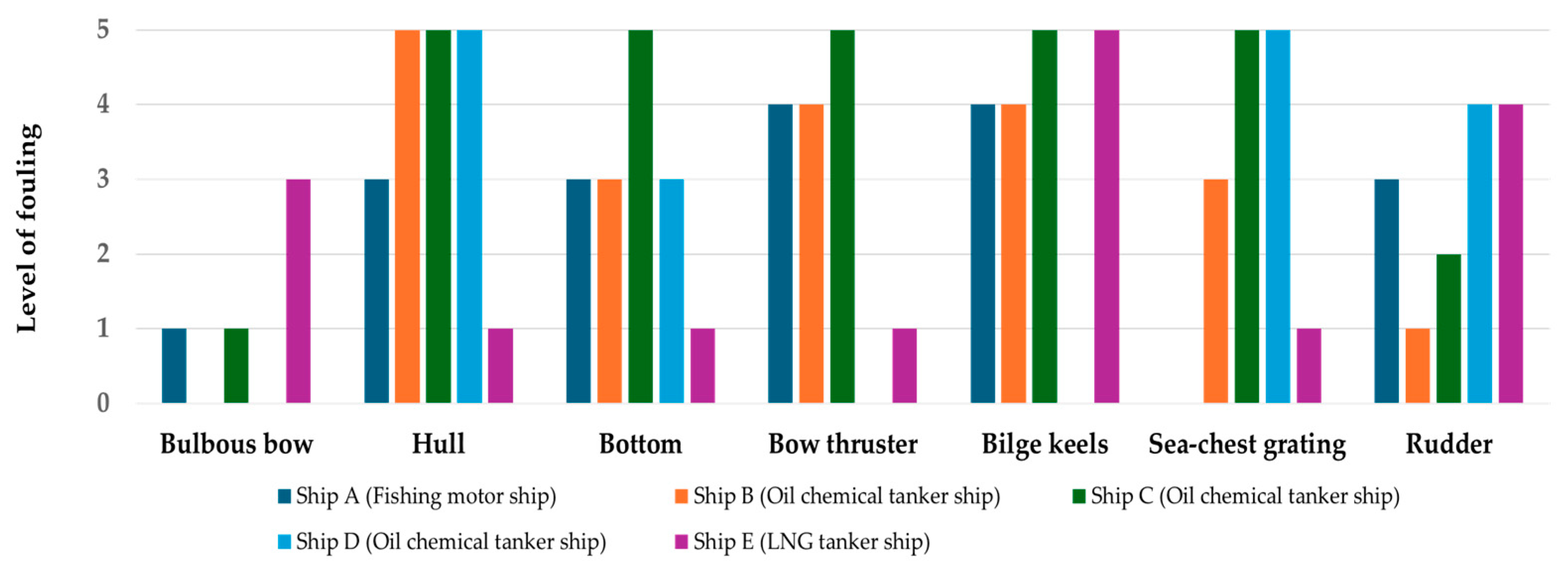
Bio-fouling occurs on all ship structures, including propellers, bilge keels, and anchors, and exhibits different growth rates in various areas of the ship [19]. Park (2022) assessed the classification of bio-foulings in five domestic and international ships (A: fishing motor ship, B–D: oil chemical tanker ship and E: LNG tanker ship) and identified different classifications for ship-specific areas [4]. As illustrated in Figure 1, Grades 0–3 of bio-fouling were found on the bulbous bow compared to other areas, whereas Grades 4–5 were observed on the hull and bottom. Particularly in niche areas, such as the side thrusters and sea chest, larger attachments of a relatively high grade (5 or higher) have been observed. Other studies have also identified niche areas as major sites for the accumulation of bio-fouling in marine ecosystems [20,21]. Therefore, it is essential to select an appropriate cleaning method and cycle according to the growth size to effectively remove bio-foulings grown in the bow thruster and sea chest. Ships typically undergo an annual inspection, an intermediate inspection every three years, and a periodic inspection along with hull cleaning at the end of five years to combat bio-fouling [22].

Figure 1.
Grading of bio-fouling by ship section (adapted from Ref. [4]).
In terms of cleaning methods, various cleaning tools have been manufactured to increase the efficiency of cleaning operations and reduce the intensity of labor. Hull-cleaning methods can be categorized based on the tools used, such as manual hull scraping with sharp tools, motor-driven rotary brushes, and non-contact methods using water jets [23]. Operators mainly apply the electric rotary brush cleaning method to large ships and select the appropriate brush type based on the bio-fouling size and adhesion. Nylon brushes remove micro-fouling, such as seaweed and bacteria, and are used in steel brushing to remove macro-fouling. However, using a stiff metal brush can significantly damage not only the bio-fouling but also the paint surface of the hull. Therefore, an appropriate brush material must be selected based on bio-fouling growth. Non-contact cleaning methods mainly involve high-pressure and cavitation water jets. Unlike cleaning methods using brushes, high-pressure water jets spray high-pressure spinal water on the hull. This method removed bio-fouling without damaging the hull. However, if the bio-fouling is large, there is still a possibility that the hull will be damaged when the fouling disconnects, owing to the sprayed pressure [13]. The cavitation water-jet method involves inducing forced cavitation phenomena in the jet flow, which significantly increases the local shear stress owing to explosions occurring during the cavitation growth process, thereby removing bio-fouling. However, owing to the rapid growth of cavitation flows, research through model testing and numerical calculations is necessary. Recently, cleaning robots capable of cleaning confined areas that are difficult for humans to reach have been developed, and active research is ongoing. Most cleaning robots use water jets and brushes for cleaning, and the status of commercially operated cleaning robots can be found in Table 2.
Table 2.
Overview of commercial in-water robotic cleaning solutions (adapted from Ref. [24]).
Considering the cleaning efficiency for large fouling organisms and the potential for paint damage, it is more appropriate to choose a cavitation high-pressure water jet over a brush. However, since the size of fouling organisms varies depending on their growth process, various factors such as pump pressure, nozzle transmission speed, and the distance between the ship and the nozzle must be considered for efficient cleaning. Therefore, for a cleaning robot using a cavitation high-pressure water jet to clean effectively, it is necessary to select the factors that can influence the removal of bio-fouling and conduct basic research to determine which factor is most dominant in the cleaning process.
In previous studies related to high-pressure water jets used for cleaning bio-foulings, Oliveira and Granhag (2019) evaluated the bio-fouling removal performance of water jets to minimize damage to the coating [25]. Subsequently, Oliveira and Granhag (2019) conducted experiments on the removal of bio-foulings adhered to anti-fouling coating (AF) and for-release coating (FR), confirming the effectiveness of removal when cleaned on a bi-monthly or monthly basis [26]. Seo and Oh (2022) conducted removal experiments using water jets on materials commonly used in small vessels in the west coast region of South Korea. They found that seaweeds, such as kelp, were removed effectively at a spray distance of 1.8 cm and a pressure of 100 bar. However, for barnacles, it was observed that cleaning required pressures exceeding 200 bar [27].
Therefore, this study aims to address the issue of effectively cleaning the niche areas of the hull that are difficult to reach with traditional cleaning methods. It focuses on non-contact cleaning robots using cavitation high-pressure water jets to identify which cleaning factors are most dominant for efficient cleaning. Through this research, we aim to evaluate the effects of various factors, such as pump pressure, nozzle transmission speed, and the distance between the ship and the nozzle, on bio-fouling removal, and to identify the dominant factors. This study serves as foundational research for the development of cleaning robots based on cavitation high-pressure water jets. It is expected to make significant contributions to solving bio-fouling issues in the marine industry and to enhance the potential for the development of commercially viable cleaning robots.
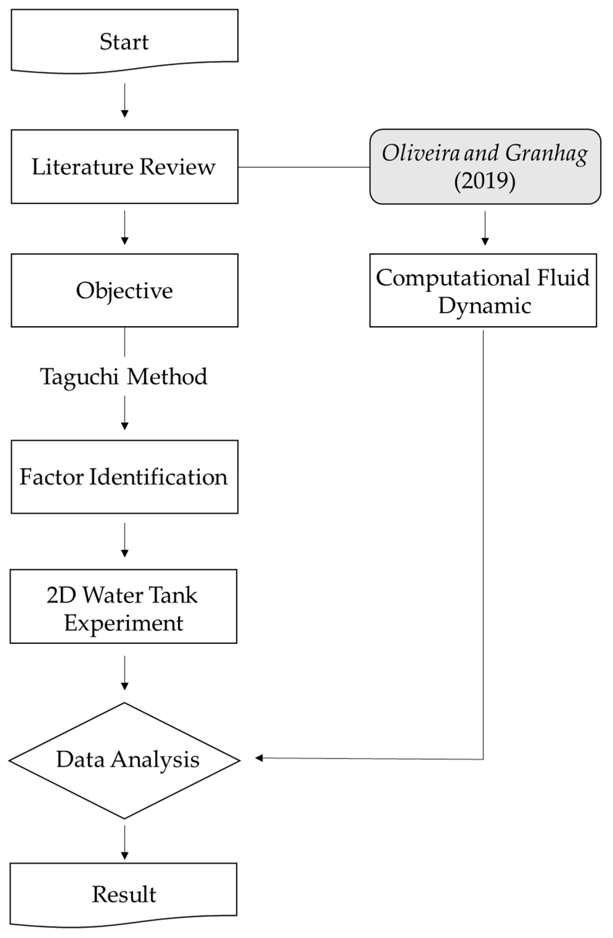
In this study, a series of experiments and analyses were conducted to evaluate the factors affecting the efficient removal of bio-fouling using cavitation high-pressure water jets. The Taguchi method was employed to identify the influential factors and generate experimental conditions, thereby establishing an efficient experimental plan. The experiments were conducted using a 2D water tank (L: 25 m, W: 1 m), with samples prepared from materials commonly used in various areas of ship hulls where bio-fouling occurs. These samples were fixed in a sample fixation frame to facilitate the growth of hull-attached organisms. Additionally, computational fluid dynamics (CFD) was utilized to perform a numerical analysis of the nozzle to evaluate the cleaning performance and shear force of the high-pressure water jet, aiming to derive the optimal cleaning conditions and quantitatively assess the nozzle’s cleaning performance. Experimental variables included pump pressure, nozzle transmission speed, and the distance between the ship and the nozzle. After the removal experiments, images of each sample were analyzed to quantitatively compare and verify the bio-fouling removal effects, ultimately identifying the dominant factors influencing cleaning efficiency. The research methodology is summarized in Figure 2.
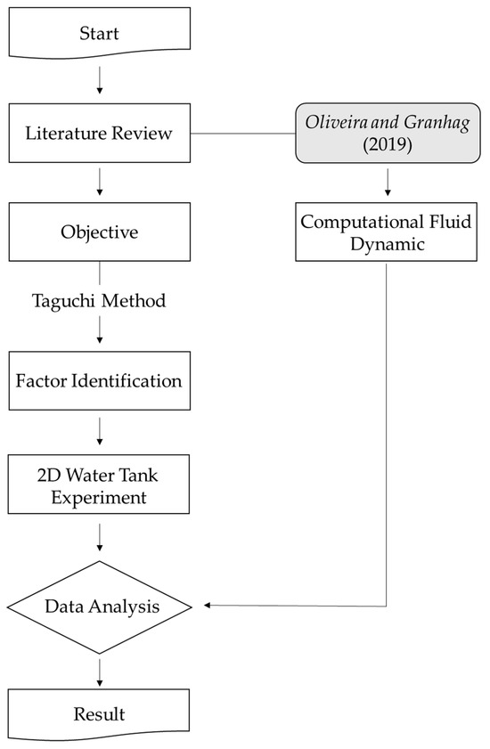
Figure 2.
Research methodology framework [25].
2. Setup of Bio-Fouling Removal Experiment
2.1. Protrusion of Evaluation Factors (Design of Experiment)
Oliveira and Granhag (2020) selected factors that influenced the cleaning performance of bio-foulings based on water jets, such as the towing carriage speed (transport speed of the nozzle), water-jet spray distance, and water-jet pump pressure. The factors were varied as follows: the towing carriage speed was less than 0.3 m/s, the spray distance was 16 or 25 mm, and the pump pressure was up to 200 bar [26]. In this study, to review the evaluation of cleaning performance more extensively than the previous study, the water-jet spray distance was 0.03, 0.05, and 0.07 m, the pump pressure was 100, 180, and 240 bar, and the towing carriage speed was 0.2, 0.25, and 0.3 m/s. Considering that each of the three factors has three levels, a total of 27 experiments would be required to cover all possible combinations. However, conducting all these experiments would be deemed inefficient.
Design of experiments (DOE) refers to planning experiments to analyze data. Experimental planning can be described as determining the factors that influence a product’s characteristics and finding the most economical methodology to determine whether the data obtained can only be analyzed statistically to obtain the most information. Although there are many experimental design methods, one of the most effective is the Taguchi method, which accurately identifies and objectively evaluates the impact of critical factors on data owing to noise factors such as uncontrollable environmental conditions or mechanical defects that are difficult to control [28]. In the Taguchi method, the orthogonal array is used to set up various combinations of factors, allowing for a reduced number of experiments while still including all factors when there are many variables. This approach enables the implementation of a fractional factorial design. An orthogonal array table is a preconstructed table in which each column is arranged to ensure orthogonality, meaning that the entire set of levels in one column appears the same number of times for a given level in another column. When using an orthogonal array, calculating factor variations from experimental data is straightforward, and creating and analyzing variance tables is convenient. Orthogonal array tables come in two-level and three-level designs. In this experiment, assuming two repetitions, nine experimental factor variations can be accommodated using a three-level design. The three levels are denoted as 0, 1, and 2, and the corresponding levels for each factor are summarized in Table 3. A three-level orthogonal array table is represented as shown in Equation (1) [29], where “m” represents an integer greater than or equal to 2, “3m” denotes the size of the experiment, and “(3m − 1)/2” signifies the number of columns in the orthogonal array table. In the case of a three-level design, the smallest orthogonal array table is L9 (34), which is equivalent to Table 4, and since there are three factors, “X4” is excluded.
Table 3.
Translated to levels of each experimental factor.
Table 4.
Generation of experimental conditions for biofouling removal.
2.2. Specimen Fabrication
The materials selected for bio-fouling colonization were copper, high-density polyethylene (HDPE), and iron coated with anti-fouling paints 1 and 2. However, in the case of iron, corrosion increases over time when exposed to seawater with high acidity and salinity, inhibiting the visual identification of bio-foulings during subsequent collection. Consequently, it has been replaced with STS304 stainless steel, an austenitic material known for its corrosion resistance that is commonly used in industrial settings. Copper, which is known for its excellent corrosion resistance and high strength, is used extensively in propeller manufacturing, commercial ships, and large naval vessels. For the HDPE specimens, HDPE was selected for recreational or fishing vessels, considering environmental concerns upon disposal, especially for fib-reinforced plastic (FRP) ships. The anti-fouling paint specimens were surface-treated with smooth sandpaper, as shown in Figure 3. Degreasing was performed using an auto cleaner (ZY 0950) and a soft surface. Additionally, they were coated with a tin-free SPC anti-fouling paint (A/F 795-Red brown), which is less harmful to the marine environment, considering the restrictions on the use of conventional toxic anti-fouling paints. While the thickness of anti-fouling paint coatings may vary among manufacturers, it is generally recommended to be approximately 100 μm. In this study, considering the potential paint wear during ship operation, we conducted painting work with thicknesses of 50 μm (one coating) and 100 μm (two coatings) with the assistance of KOSTEC Co., Ltd. (located in Gunsan, Republic of Korea) and Samkang S&C Co., Ltd. (located in Incheon, Republic of Korea).
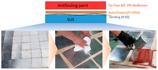
Figure 3.
Process of anti-fouling paint specimen preparation.
As illustrated in Figure 4, during the specimen manufacturing process, the specimens were designed as squares with dimensions of 0.2 m. A total of 24 specimens were securely affixed to a single-frame fixture organized in a four-column, eight-row configuration. In total, seven frames were manufactured, resulting in the installation of 168 specimens: specimens coated with anti-fouling paint one coating (×56), specimens coated with anti-fouling paint two coatings (×56), copper specimens (×42), and HDPE specimens (×14). To prevent confusion during the experiments due to the large number of specimens, each group of specimens, namely copper, HDPE, and those coated with anti-fouling paint, was designated as Cu, HDPE, K1 (one coating, KOSTEC), K2 (two coatings, KOSTEC), S1 (one coating, Samkang Shipyard), and S2 (two coatings, Samkang Shipyard). Identification was facilitated by labeling the specimens with names and numbers on their backs.
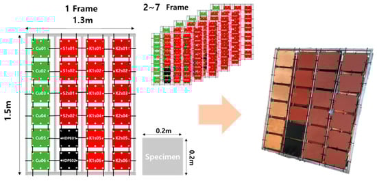
Figure 4.
Frame for fixing specimens (0.2 × 0.2 m2 specimens were used).
2.3. Bio-Fouling Cultivation
The growth stages of biofouling in marine environments transition from the micro-fouling stage, characterized by thicknesses of less than 1 mm and include organisms such as bacteria, to the macro-fouling stage, with thicknesses exceeding 1 mm and encompassing algae, barnacles, and larvae [30,31].
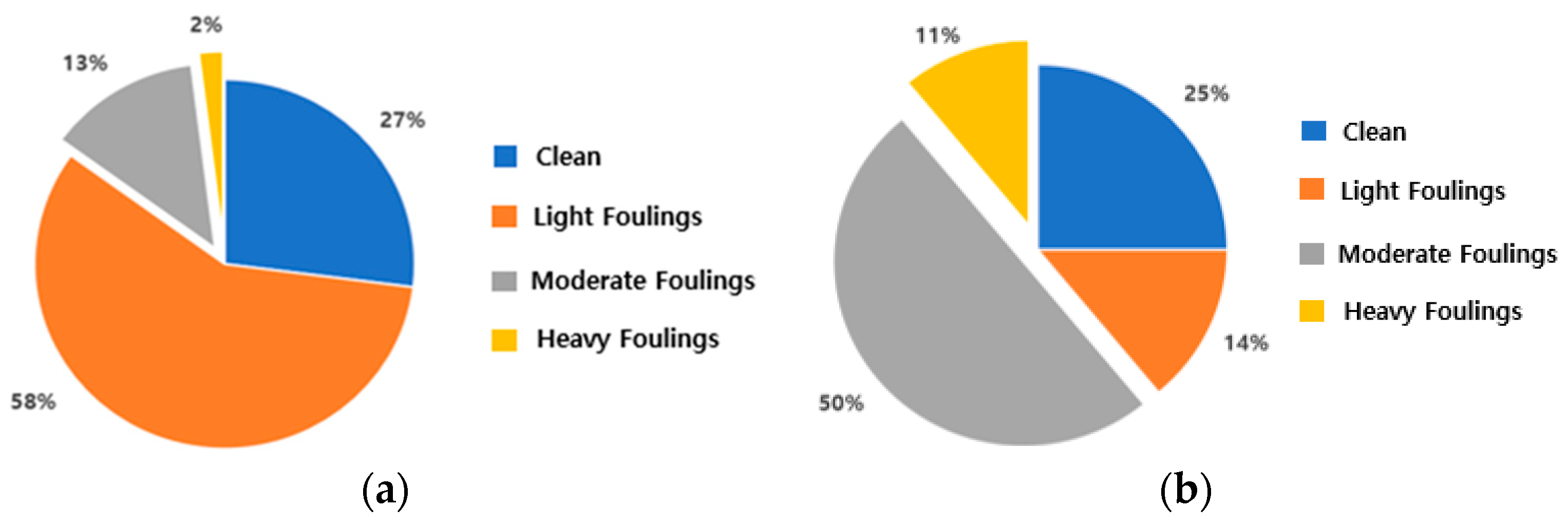
Figure 5 presents a compilation of bio-fouling colonization distribution data throughout vessel berthing, as reported by the U.S. Naval Institute in Maryland (1952). When a ship is berthed for 1–2 months, micro-fouling (light fouling) accounts for approximately 15% of the distribution. However, this proportion increased to 61% after 3–5 months of berthing, indicating a general trend of the macro-fouling (moderate, heavy fouling) growth stage commencing after approximately three months [32]. Based on this inference, a colonization period of three months (20 July 2022 to 26 October 2022) was selected for this study.

Figure 5.
Size and quantity of bio-fouling on ships relative to the duration of anchorage in port using data from the U.S. Naval Institute in 1952: (a) 1–2 months spent in port; (b) 3–5 months spent in port (adapted from Ref. [30]).
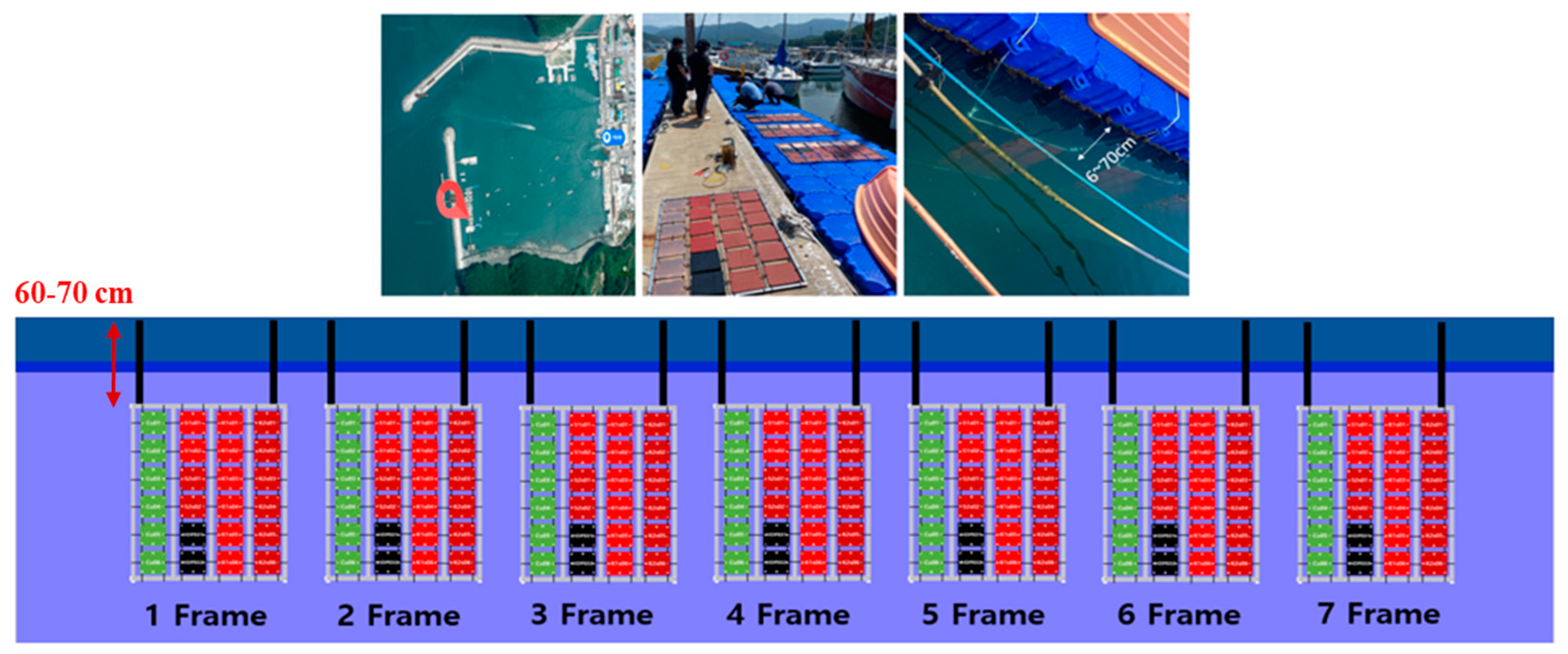
The location of bio-fouling colonization was Kyeokpo Port, located within the Republic of Korea. As depicted in Figure 6, Kyeokpo Port is situated within the harbor, which minimizes the influence of current strength and mitigates the risk of specimen loss owing to factors such as typhoons. Additionally, the presence of modular cube floating docks ensures a consistent distance from the free surface, even during low and high tides. Seven frames were fabricated and positioned approximately 60–70 cm below the free surface. The frame retrieval intervals were conducted every two weeks, following the hull surface management approach, to minimize anti-fouling damage and effectively prevent bio-fouling, as recommended by Hearing et al. (2015) [33]. The size of bio-foulings is influenced by various factors in different marine areas, such as water temperature, salinity, and density. Therefore, in future studies, when the scope is expanded, data collection will likely be necessary to analyze the growth of bio-foulings in specific regions.
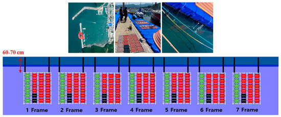
Figure 6.
Bio-fouling curing location at the Kyeopo port and arrangement of frames (positioned approximately 60–70 cm below the free surface).
2.4. Removal Experiment System Establishment
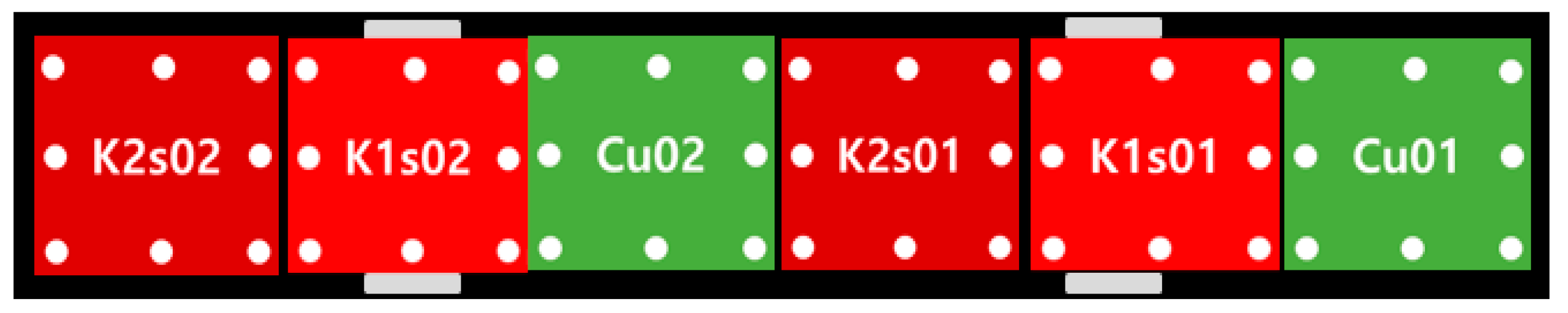
A fixing plate and test-fixing jig were constructed to secure the specimens within the 2D water tank. The design and fabrication were conducted by the Korea Research Institute of Ships and Ocean Engineering (KRISO). The bio-fouling removal experiment was conducted at the Wave Experiment Building of Kunsan National University. Specimen frames were retrieved at two-week intervals, with initial photographs of the specimens taken before the experiment to ascertain the growth stages of the bio-foulings. Subsequently, six specimens were aligned onto a fixed plate. Regarding the potential damage of the labeled names of each specimen from the pump pressure of the water jet during the experiment, there could be confusion during the post-experiment classification. Thus, the order of the experimental specimens was determined, as shown in Figure 7. In the case of specimens S1 and S2, the size of the mature bio-foulings increased because of the absence of additional anti-fouling paint on the back, presenting a limitation in fixing plate installation. Therefore, S1 and S2 were used to verify the effectiveness of the anti-fouling paint by comparing the maturation distributions before and after the bio-fouling removal experiment with K1 and K2. For the HDPE specimens, the experimental setup was arranged separately, considering a 0.02 m height difference and the spray distance between the nozzle and the specimen.

Figure 7.
Arrangement of specimens.
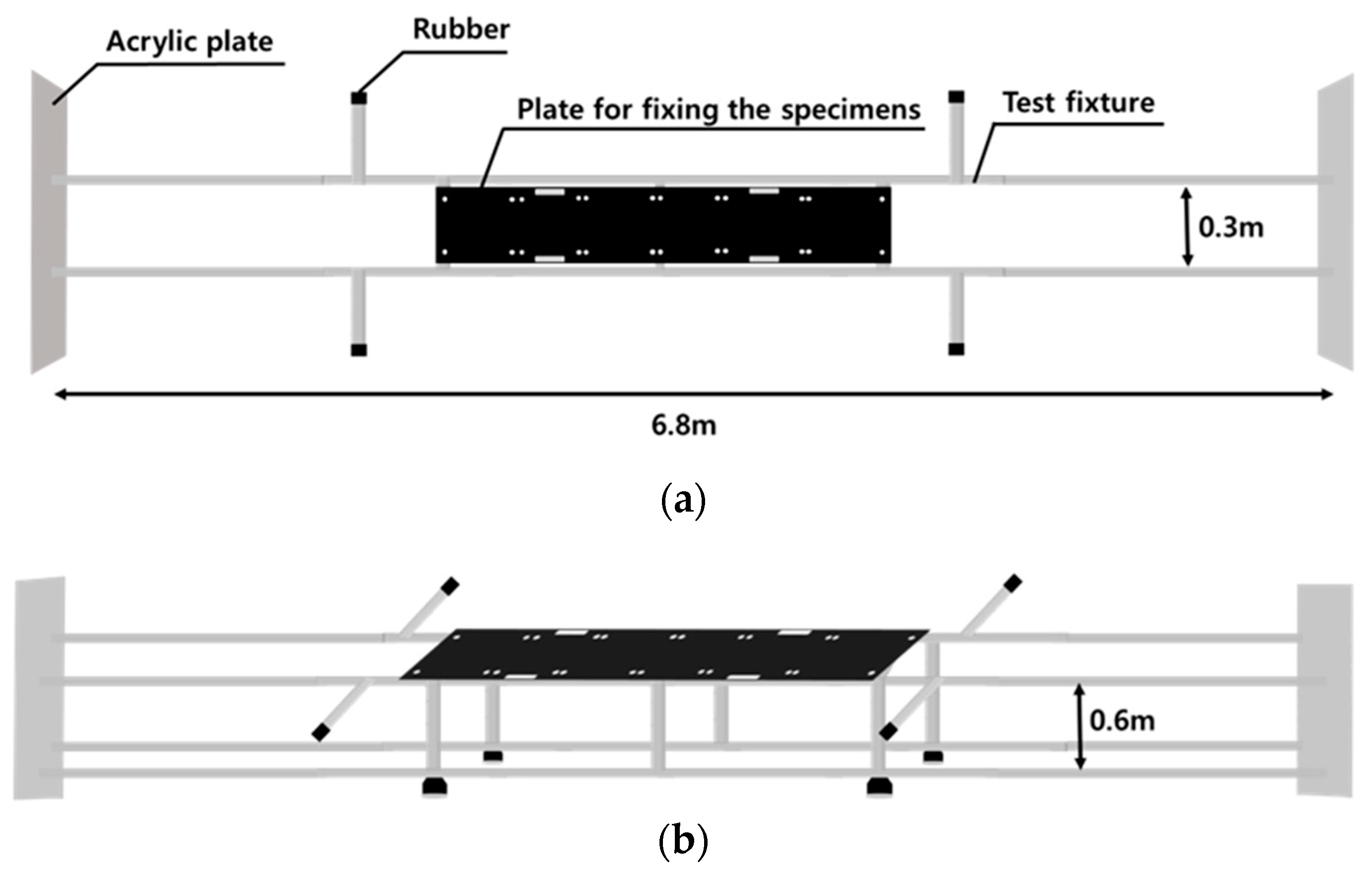
Additionally, the test-fixing jig used to secure the fixing plate is shown in Figure 8. It is made of aluminum profiles with dimensions of 6.8 m in length, 0.3 m in width, and 0.6 m in height. After the experiment, when it became necessary to replace the water in the tank due to contamination, cleaning posed limitations due to the length of the major axis of the tank. This issue was addressed by installing acrylic plates in front of and behind the test-fixing jig, considering the movement range of the towing tank.

Figure 8.
Test fixture: (a) top view; (b) isometric view.
As depicted in Figure 9, the setup consists of a water-jet injector-fixing device and a high-pressure pump, both secured to a towing carriage. The injector-fixing device was designed for movement in both vertical and horizontal directions, facilitated by sliding guides and bolt fastening. A structure with two plates bolted to the injector holder was designed to prevent the movement of the injector owing to high pressure. This structure allows for height adjustment of the injector using a block with a 5 mm elevation. The water-jet injection pump used in the experiment was a high-pressure mobile pump capable of injecting at a maximum pressure of 303 bar and a flow rate of 15 L/min. It is constructed of wheels and operates as an internal combustion engine using gasoline, which enhances its mobility.
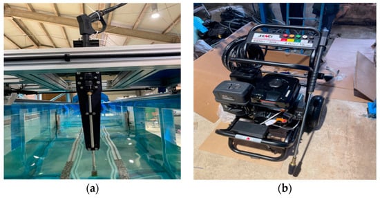
Figure 9.
Setup for the experiment on bio-fouling removal: (a) water-jet fixture; (b) high-pressure pump.
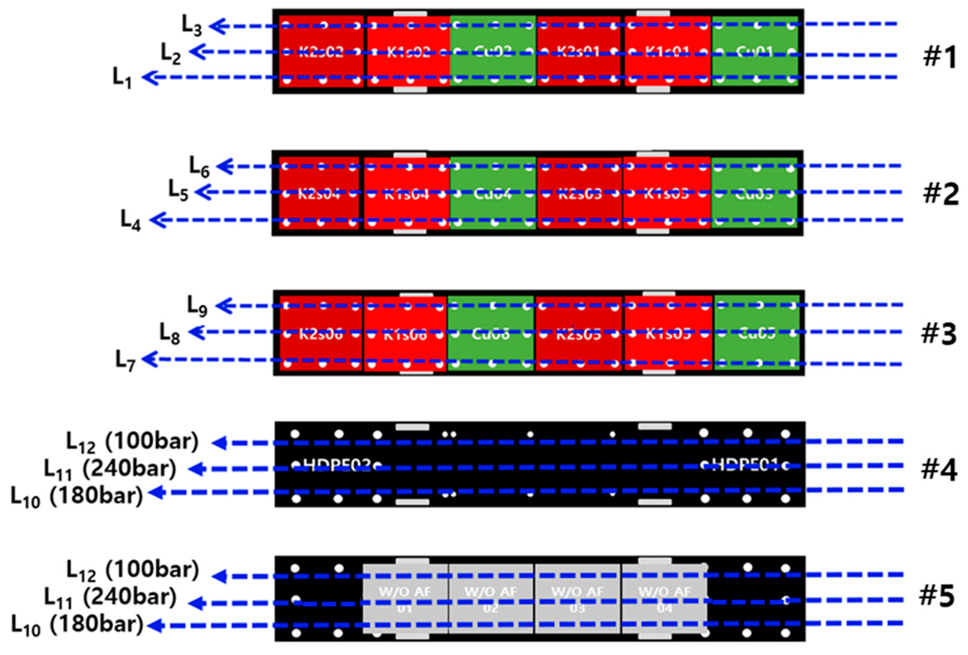
The experiment was conducted in accordance with the conditions calculated using the Taguchi method, as shown in Figure 10. Additionally, for the specimens that did not have anti-fouling paint applied and for HDPE, experiments were carried out by setting the speed of the towing carriage and the spray distance at 0.2 m/s and 0.03 m, respectively. This setup was used to conservatively evaluate the effectiveness of bio-fouling cleaning under various pump pressures. This allowed for the performance of five experiments per session during the removal test.
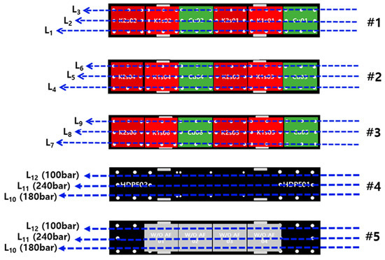
Figure 10.
Experiment plan for removal of bio-fouling.
3. Results of Experiments on Bio-Fouling Growth and Removal
3.1. Analysis of Major Emerging Species Based on the Cultivation Period
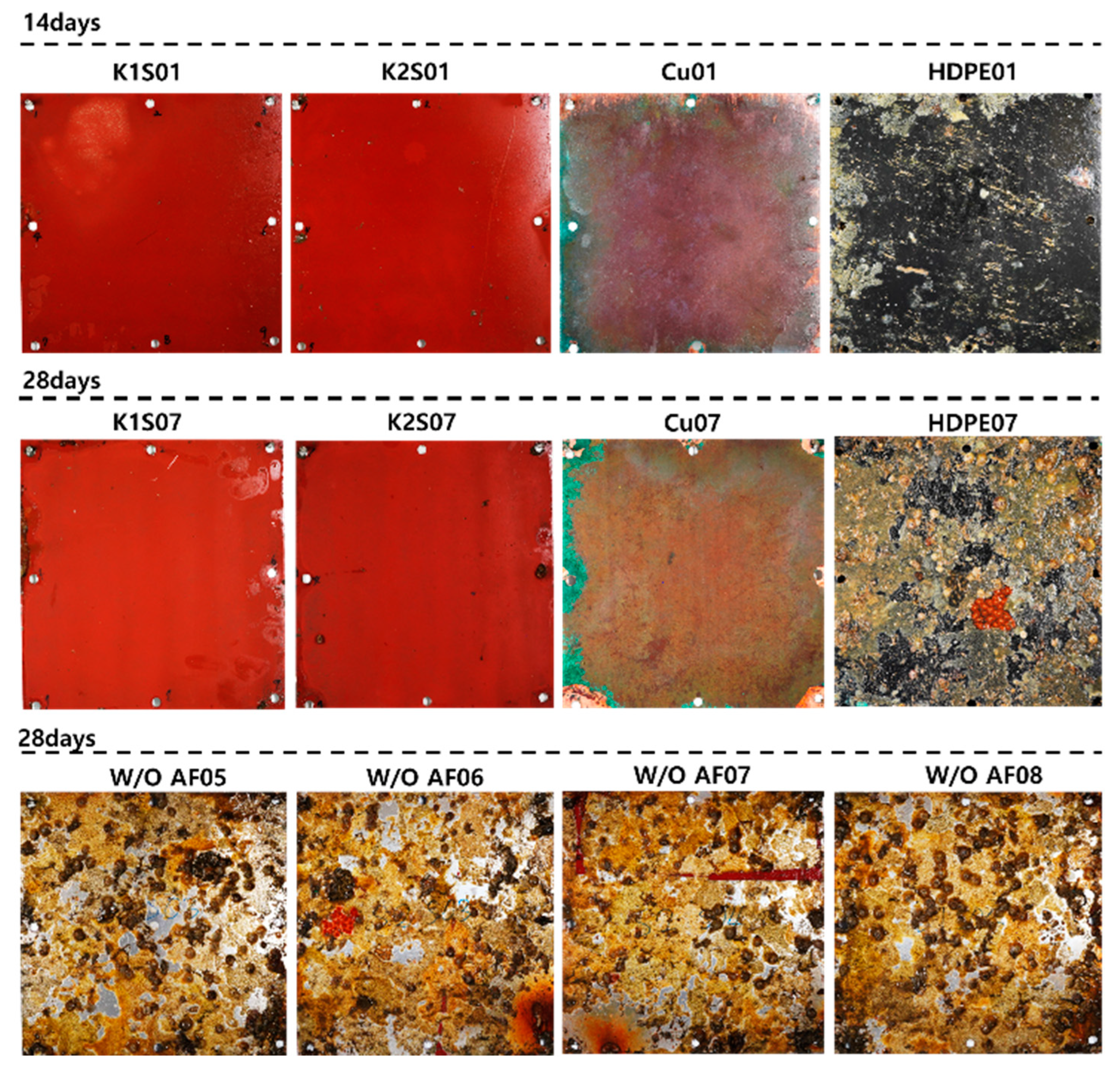
Figure 11 lists one representative specimen each from those cured for 14 and 28 days, along with specimens not coated with anti-fouling paint. In the K1 and K2 specimens, no bio-foulings were visible to the naked eye. For copper, minute corrosion appeared on the corners by day 14, and some fragments were observed by day 28. Generally, copper is a chemically stable metal and does not react with seawater, but prolonged exposure can accelerate corrosion processes due to the reaction of seawater’s chloride ions with copper to form copper chloride. Additionally, copper suboxide (CuO), one of copper’s oxides, causes reproductive toxicity and is used in organisms to prevent bacterial reproduction. For instance, a copper rod in an aquarium can prevent crustacean or cephalopod shell formation, or brass products are applied to handles for viral prevention through their antibacterial effects. Thus, like the specimens coated with anti-fouling, bio-foulings were observed on the Cu specimens. However, traces of coral were evident on the HDPE specimens by day 14, and by day 28, colonial ascidians and barnacles began to grow, suggesting that a level 5 of heavy macro-fouling could be expected by the end of the curing period. Specimens without the anti-fouling coating, when immersed in seawater for 28 days on the back of S1 and S2 specimens, showed many bio-foulings in the form of seaweed, indicating the significant role of the anti-fouling agent. Observing the adherent bio-foulings on each specimen cured in seawater for 14 and 28 days and those without anti-fouling paint, as shown in Figure 11, large adherent bio-foulings like barnacle clusters and pneumocysts did not appear. However, small barnacles were observed on the specimens without HDPE and anti-fouling paint. Nevertheless, more mature adherent bio-foulings were needed to analyze the removal effect of the water jet in this study; hence, a removal experiment was conducted on specimens cured from day 42 onwards.
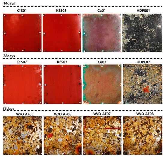
Figure 11.
Specimens on 14 and 28 days.
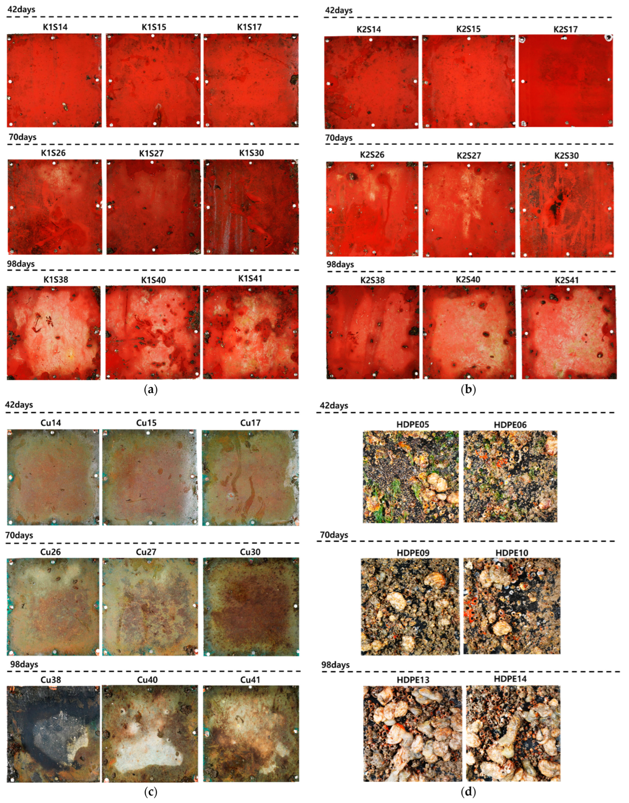
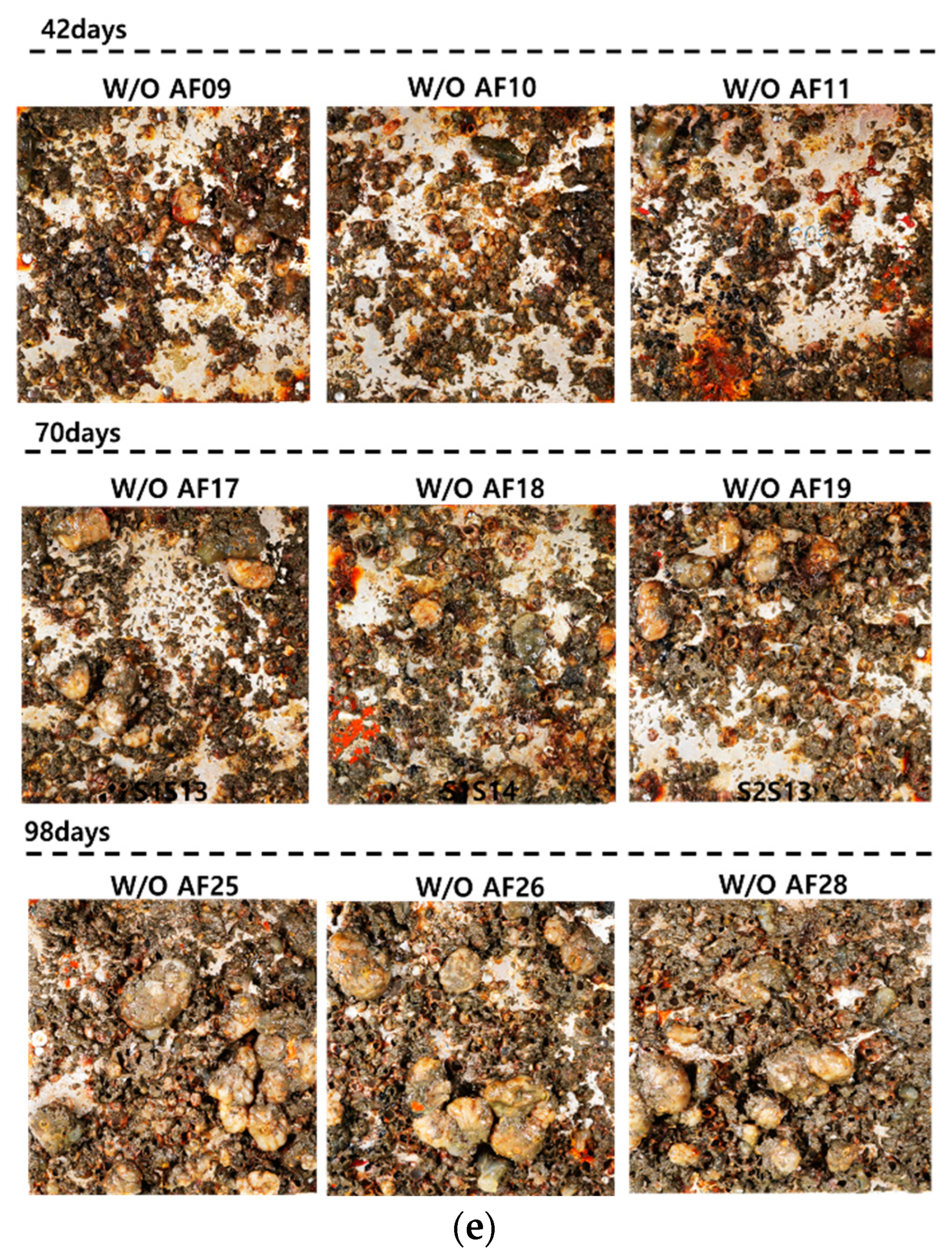
Figure 12 shows each specimen cured for 42, 70, and 98 days. The K1 and K2 specimens, compared to those cured for 14 and 28 days, appeared to be relatively contaminated but did not exhibit macrofouling of large, attached bio-foulings. The specimen without anti-fouling paint grew into a barnacle cluster by day 42, and large capsules were scattered on days 70 and 98. Compared to the K1 and K2 specimens during the same curing period, many bio-foulings grew on the surface. This reiterates the effectiveness of anti-fouling agents in preventing bio-foulings. For the Cu specimen, severe abrasion occurred at the edges as the curing progressed, inhibiting visual confirmation of the damage. Therefore, it is necessary to consider using a material with a special coating that protects or prevents corrosion when copper is exposed to seawater for three months or more. As mentioned earlier, in the HDPE specimen, barnacle clusters and some large cysts grew on the surface after 42 days. By the last 98 days, the surface of the specimen was covered with bio-foulings, which made it difficult to see, indicating the need for the periodic cleaning of small fishing boats and warships made of HDPE.


Figure 12.
Specimens on 42, 70, and 98 days: (a) K1; (b) K2; (c) Cu; (d) HDPE; (e) W/O AF.
3.2. Results of the Bio-Fouling Removal Experiment
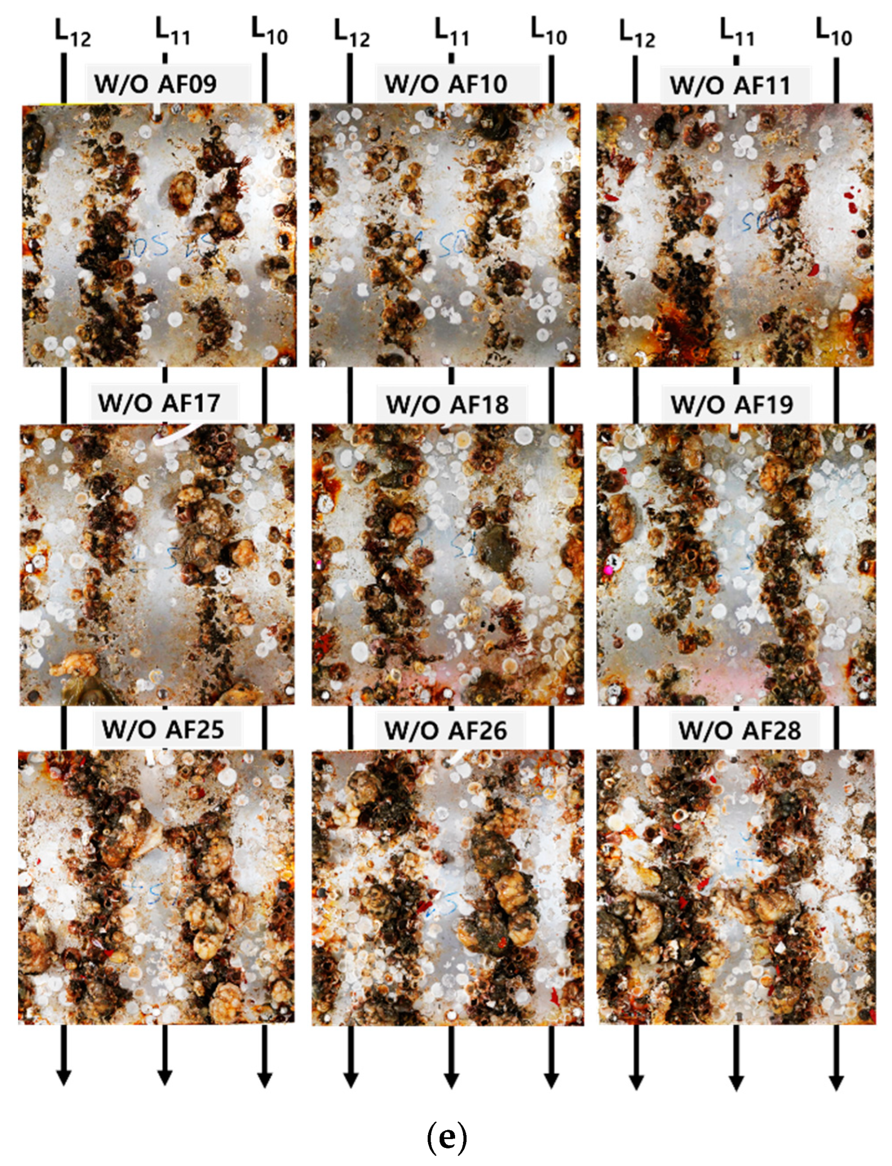
Figure 13 shows each specimen cleaned after the removal experiment was conducted for 42, 70, and 98 days. In specimens K1 and K2, the surfaces appeared relatively smoother after cleaning when observed with the naked eye. However, aside from the removal effects, it was noted that in the K1S26 specimen, under the experimental condition L3 (pump pressure 240 bar, spray distance 0.03 m, and towing carriage speed 0.3 m/s), the anti-fouling paint chipped off more than under other conditions. Particularly in the more mature K1S38 specimen, paint chipping was observed not only in condition L1 but also in conditions L2 and L3, suggesting that the growth of bio-foulings and their root embedment in the paint may have accelerated the damage post-cleaning. Therefore, additional paintings may be necessary during postoperative inspections of ships. Specimens that were not coated with the anti-fouling paint were tested under fixed conditions of spray distance 0.03 m and towing carriage speed 0.2 m/s, varying only the pump pressure. On day 42, most bio-foulings were removed under all pump pressure conditions; however, in the W/O AF09 specimen, some pneumocysts remained unremoved, even at 240 bar, indicating the need for a high-pressure water jet over 240 bar to clean large bio-foulings at a 0.03 m spray distance. After 70 days, all the specimens appeared clean, and on day 98, only the W/O AF28 specimen at 100 bar remained uncleaned. Similar to K1, copper peeling was observed in the Cu26 and Cu28 specimens. Conversely, the twice-painted (100 m) K2 specimens did not show paint chipping under condition L3, indicating only bio-fouling removal. This suggests the need for further research to determine the optimal cleaning conditions based on curing duration and paint thickness. In the HDPE specimens, partial cleaning was observed for up to 70 days under condition L12 (pump pressure of 100 bar). However, large pneumocysts, such as the HDPE05 specimen, were not removed. On day 98, the barnacles remained in the 100 bar area, and in the 240 bar area, numerous pneumocysts prevented effective cleaning.
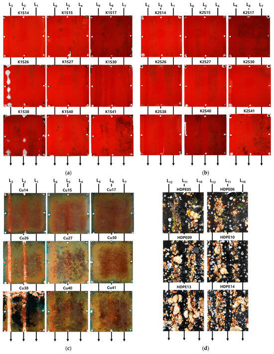
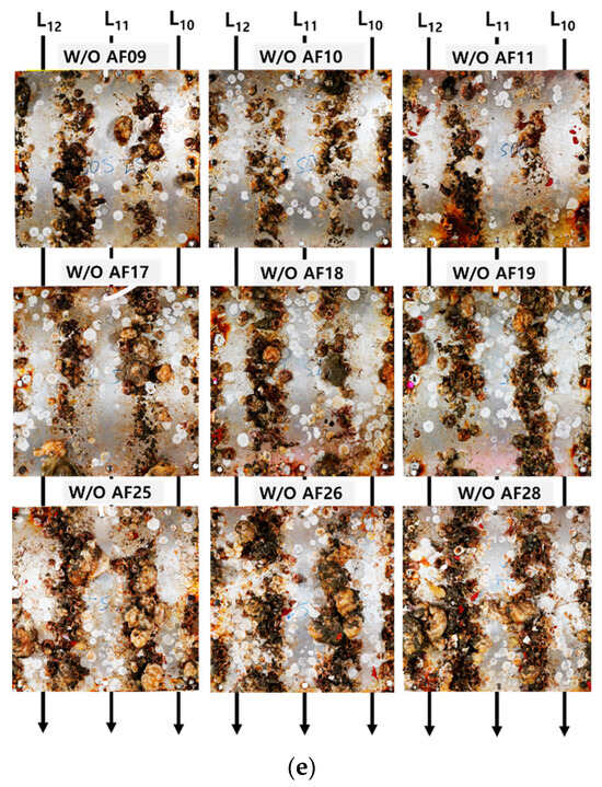
Figure 13.
Specimens after cleaning on 42, 70, and 98 days: (a) K1; (b) K2; (c) Cu; (d) HDPE; (e) W/O AF.
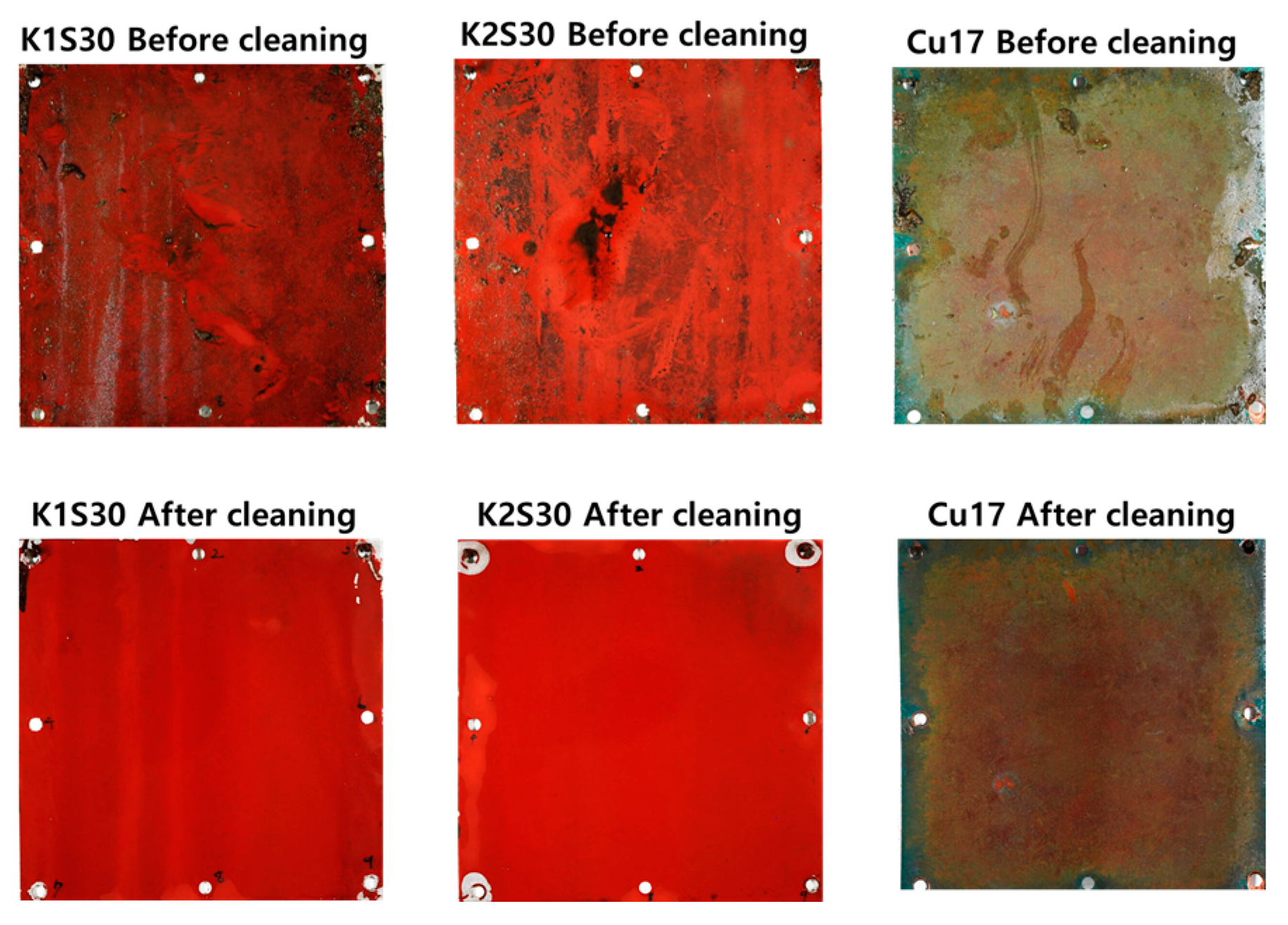
Based on the results before and after the bio-fouling removal experiments, it was intuitively confirmed that macro-fouling had grown on the HDPE and W/O AF specimens, demonstrating the effectiveness of the cleaning process. However, as shown in Figure 14, for the K1, K2, and Cu specimens, which were still in the micro-fouling stage at 98 days, it is difficult to clearly determine the cleaning effectiveness of the high-pressure water jet. Although the surface appeared smoother post-cleaning, indicating the removal of sand, there are limitations in visually confirming the removal of micro-fouling. While the cleaning effect can be confirmed through image analysis in the factor evaluation section, it is necessary to analyze the force exerted by the water jet used in this experiment on fouling removal. Therefore, in the next section of this study, numerical analysis was conducted to estimate the forces, such as stagnation pressure and wall shear stress, exerted by the high-pressure water jet to verify its cleaning effectiveness on bio-fouling.

Figure 14.
Visual comparison of specimens before and after cleaning at 98 days.
4. Numerical Analysis of the Cleaning Effectiveness on Bio-Fouling
4.1. Nozzle Numerical Analysis
This study used the commercial program STAR-CCM+ (Ver. 15.06), based on the finite volume method, to estimate the internal average flow velocity of the nozzle used in high-pressure water jets and calculate the cleaning forces (stagnation pressure, wall shear stress) for each spray distance. One of the prominent numerical methods for capturing turbulent jet flows is the Large Eddy Simulation (LES) model. LES enhances computational efficiency and accuracy by directly simulating large eddies and modeling small eddies within the flow. In relevant prior studies, Ningegowda et al. (2020) employed the LES model to analyze the mixing of ambient nitrogen under supercritical conditions, validating the numerical implementation’s accuracy [34]. Xiao et al. (2016) simulated the primary breakup processes of a liquid jet in a supersonic air crossflow, investigating the interactions between gas and liquid phases [35]. Additionally, Gohil et al. (2014) used the LES model to analyze the turbulent characteristics of jet flow at a Reynolds number of 10,000, confirming its utility in accurately predicting the turbulent properties of a free circular jet. Their results showed good agreement between time-averaged velocity profiles, turbulence statistics, and experimental data, thereby validating the effectiveness of the LES model [36]. However, the LES model is computationally intensive due to the need for finer grids and smaller time steps to directly resolve large eddies and model small eddies. In contrast, the RANS model is computationally more efficient and provides sufficient accuracy for many practical engineering applications, such as internal flows in pipes and ducts, and external flows around vehicles and structures [37,38]. Therefore, this study employs the RANS model for the numerical analysis of the nozzle. The governing equations of the incompressible turbulent flow are the continuous equation and the Reynolds-averaged Navier–Stokes equation (RANS) equation, which are shown in Equations (2) and (3).
Here, represents the mean velocity in the x-, y-, and z-directions, and u defines the fluctuating velocity components due to turbulence in the same directions. The velocity components are nondimensionalized by the inflow velocity , and the spatial coordinates x, y, z are nondimensionalized by a characteristic length L (inner diameter of nozzle). Similarly, the pressure is nondimensionalized using . Consequently, the Reynolds number is denoted as .
Considering the pump’s performance with a maximum pressure of 303 bar, a flow rate of 15 L/min, and a nozzle diameter of 0.2 cm, the Reynolds number inside the nozzle is approximately 1.40 × 10⁵, indicating highly turbulent flow. Therefore, it is essential to apply a turbulence model in the simulation. In this analysis, improved results in flow, such as swirls and peeling with complex shear flow and strain rate, were shown, and an RNG k-ε turbulence model that was already validated and verified was used. In addition, the pressure–speed coupling method uses the semi-implicate method for pressure-linked equations (SIMPLE) to analyze the pressure coupling equation. This has the advantage that the velocity field corresponding to the pressure field converges during the iteration, thus reducing errors in the numerical calculation and calculation time.
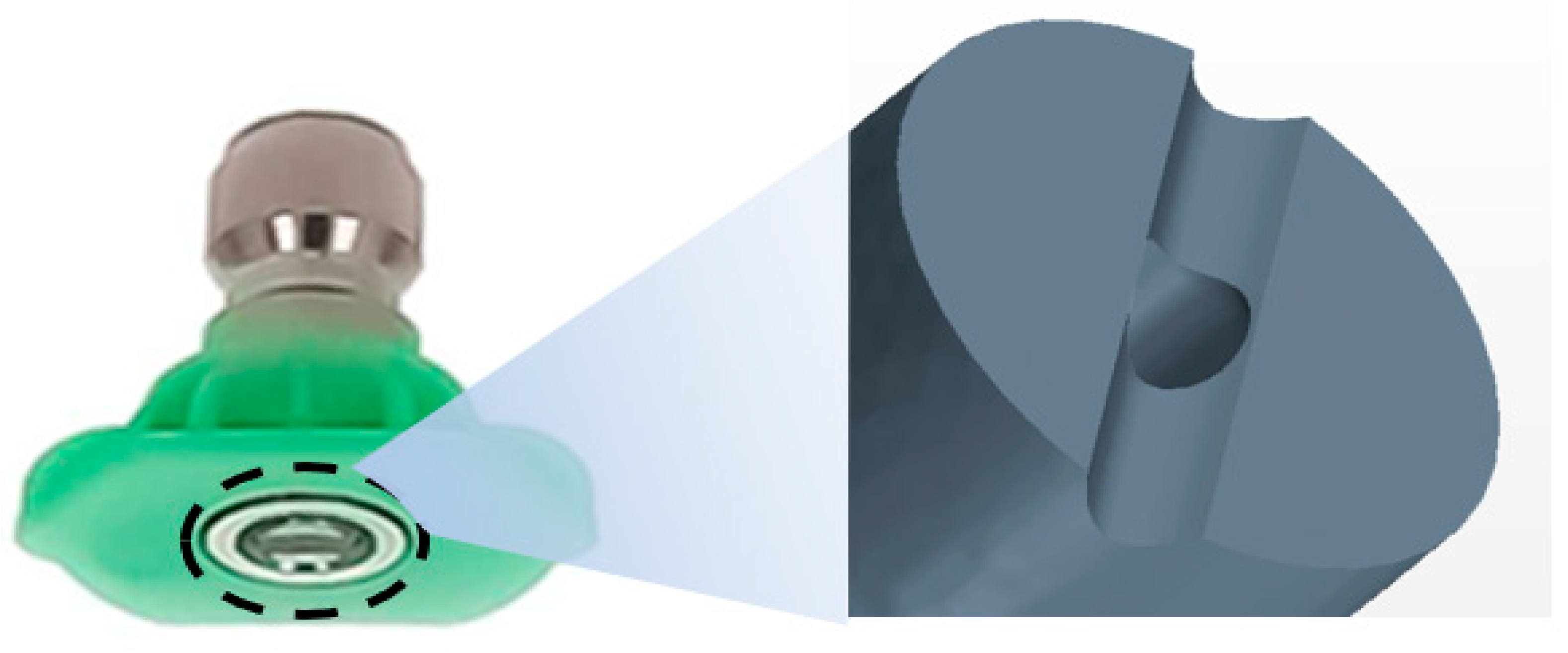
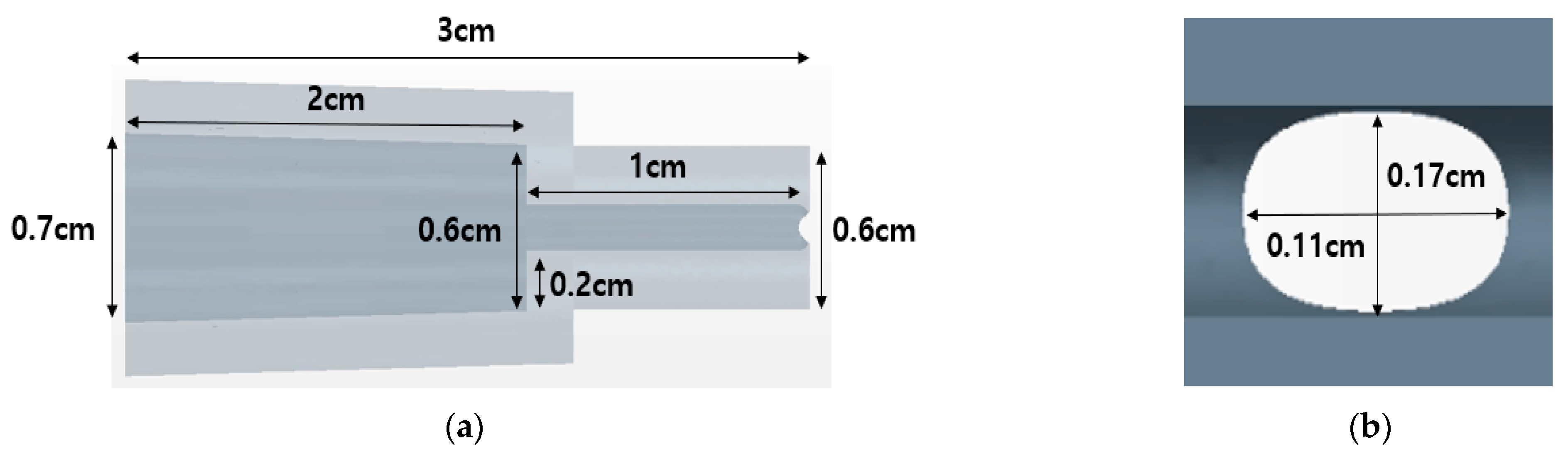
The target nozzle model used in this analysis employed a nozzle tip at 25° intervals, as shown in Figure 15. The cross-section is oval, has a short axis (1.1 mm) and a long axis (1.7 mm) with a slit shape (0.5 mm) at the end, and an area of 1.47 × 10⁻⁶ m2. The detailed nozzle specifications are shown in Figure 16.
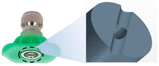
Figure 15.
Nozzle for spraying with tip 25°.

Figure 16.
Detailed dimension for nozzle: (a) side view dimensions of the nozzle interior and exterior; (b) dimensions of the nozzle inlet.
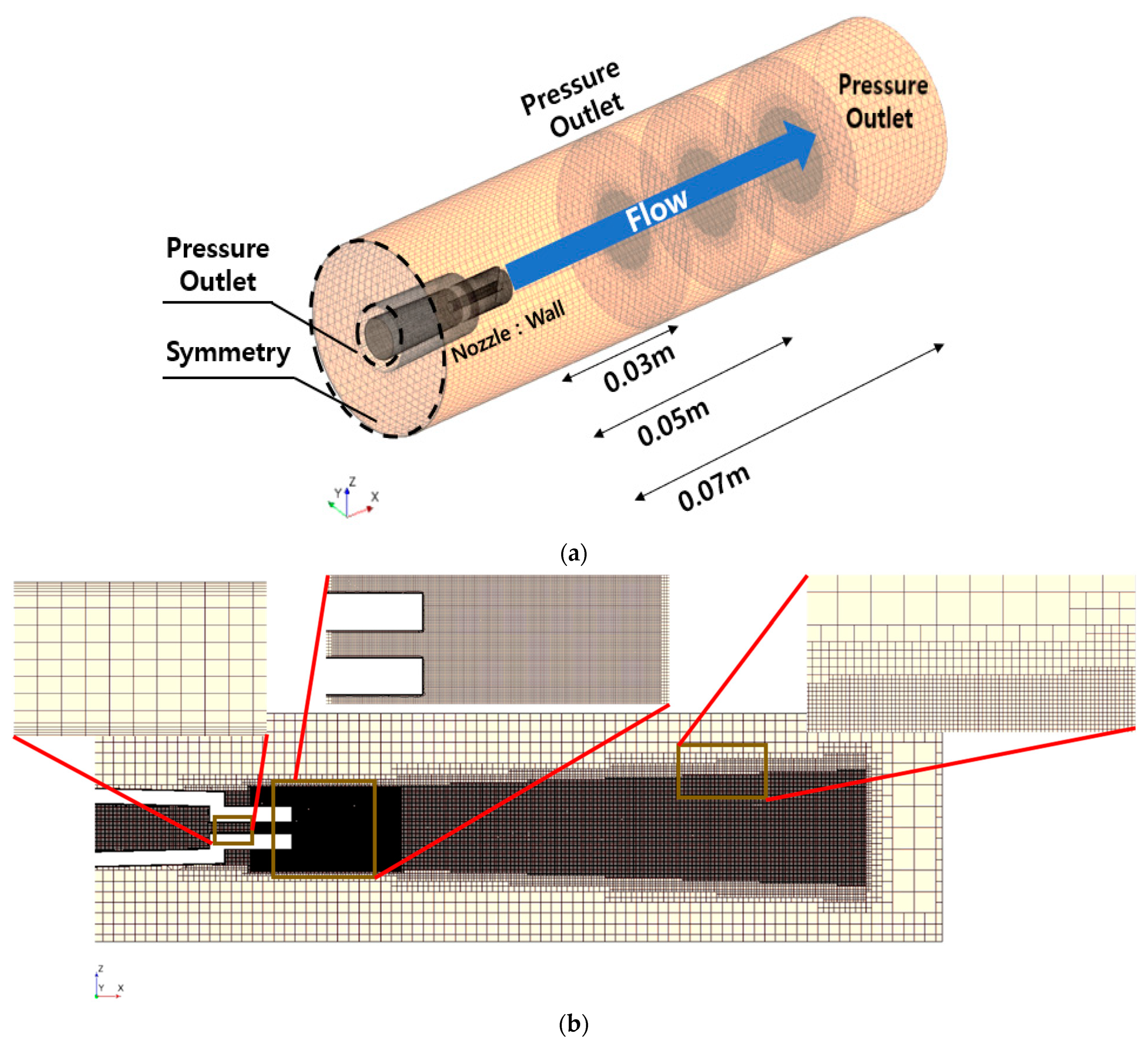
Prior to a comprehensive numerical calculation of the nozzle, a nozzle performance simulation conducted by Yang (2019) was used to establish the boundary conditions and grid [39]. The dimensions of the flow field were set at a length of 0.12 m and a width of 0.032 m. Because the nozzle operated under static pressure conditions, the nozzle inlet was designated as a pressure outlet with settings of 100, 180, and 240 bar. For the sides of the flow field, considering a future removal experiment in which the nozzle would be submerged in water, the pressure outlet was set at 1 bar.
In this simulation, the grid was formed by tetrahedra with approximately five million cells. The base size of the grid was 0.0015 m (x-direction). Five prism layers with a stacked grid thickness of 0.00015 m (y-direction) were employed to enhance the accuracy of the flow in the viscous boundary layer. Furthermore, to calculate the enhanced shear force through numerical analysis, the grid was intricately designed around the central axis, considering the inside of the nozzle tip and nozzle injection pattern. The time step (dt) was set at 1.0 × 10⁻⁶ s and the simulation time at 0.01 s to calculate the rapid flow rate (maximum 220 m/s) at the nozzle tip. Detailed information on the boundary conditions and grid system is presented in Figure 17.

Figure 17.
Domain and boundary condition and mesh for numerical calculation: (a) domain and boundary condition; (b) mesh distribution.
In a previous study, Oliveira and Granhag (2019) suggested an efficient shear force for removing bio-foulings attached to the hull to minimize damage to the anti-fouling paint by suggesting 0.17 MPa of the stagnation pressure of the water jet and 1.3 kPa of the maximum wall shear stress when cleaning the hull every other month [25], as shown in the following Equations (4) and (5).
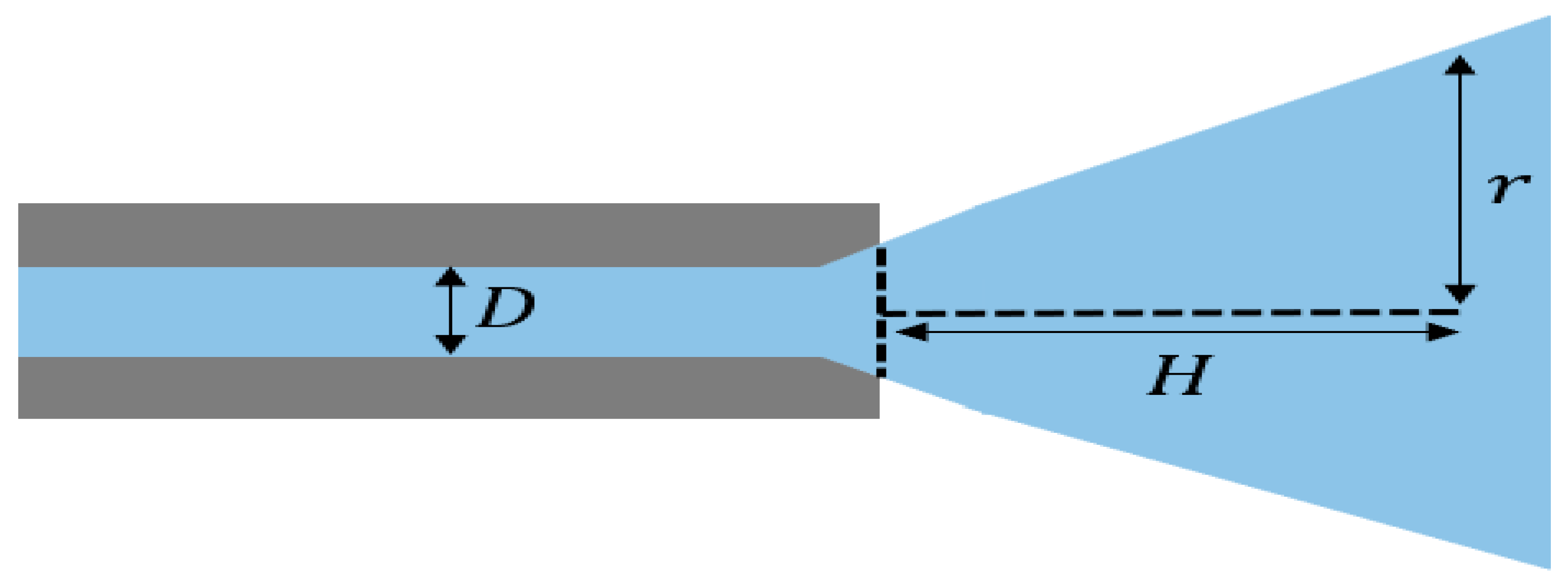
is the average flow rate through the nozzle and Re represents the Reynolds number () based on the nozzle inner diameter. D is the inner diameter of the nozzle, and H and r are the injection distance from the nozzle tip and the radius of the major axis in the injection area, respectively. The positions used to obtain the static pressure and wall shear stress are shown in Figure 18. The calculation case will analyze the injection flow rates at pump pressures of 100, 180, and 240 bar and injection distances of 0.03, 0.05, and 0.07 m with the nozzle fixed, as shown in Table 5.
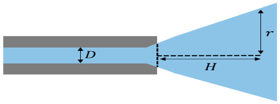
Figure 18.
Position of D (inner diameter), H (injection distance) and r (radius of injection area).
Table 5.
Cases for nozzle removal performance.
To estimate the stagnation pressure () and wall shear stress () when actual specimens are subjected to force, it is important to create walls at each spray distance for analysis. However, simulations that include wall interactions require high-resolution grids and small time intervals, which can be computationally intensive. Therefore, in this nozzle numerical analysis, we used free-flow modeling to analyze the fluid velocity of the water jet before interaction with the specimens. This approach allowed us to estimate the approximate removal forces, such as stagnation pressure and wall shear stress, as presented in Equations (4) and (5). Additionally, we conducted validation to ensure that the analytical model aligns well with experimental data, thereby providing a foundation for future research involving more complex interactions, such as jet–wall impacts.
4.2. Validation of Numerical Calculations and Determination of Average Flow Velocity
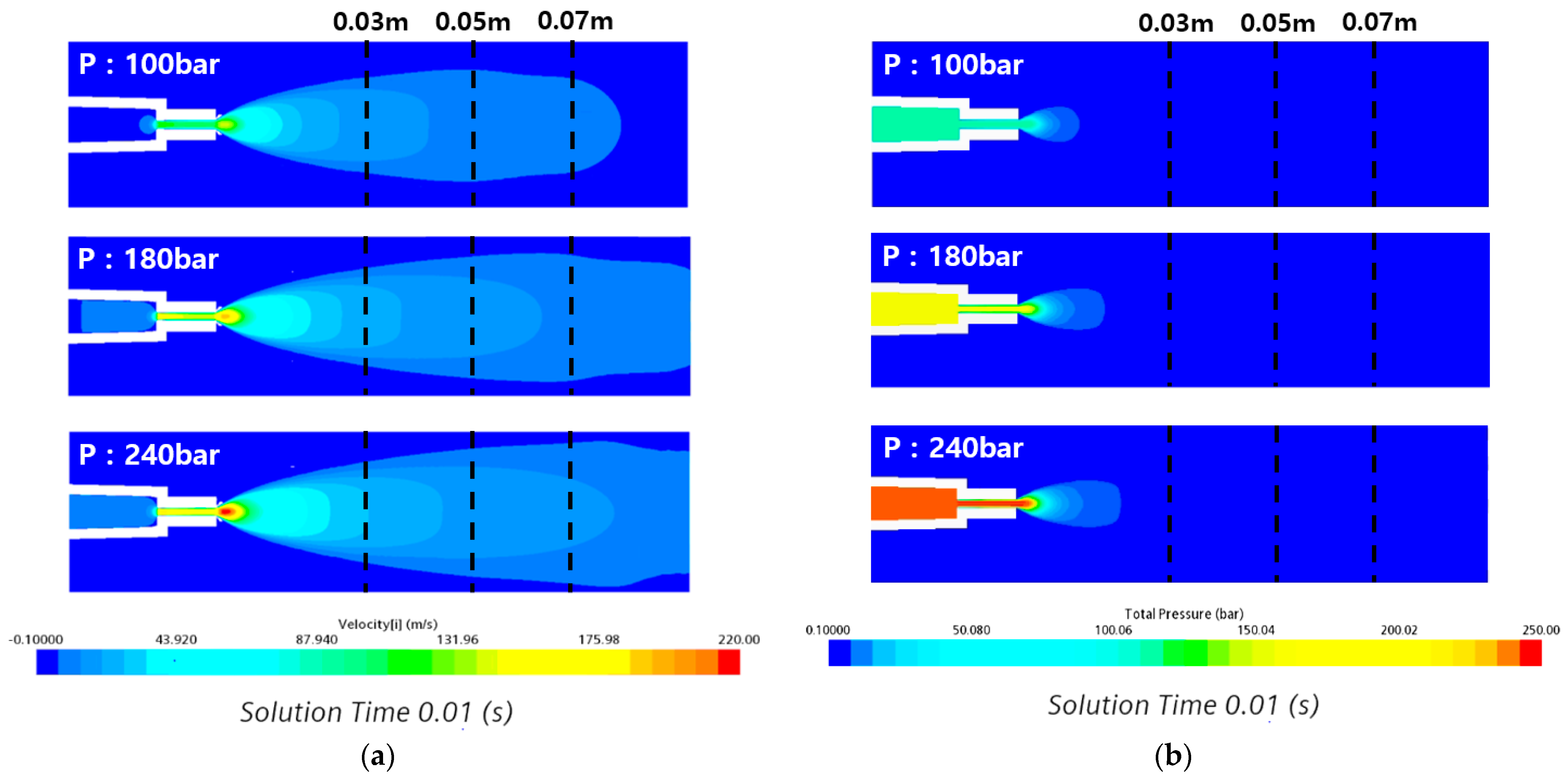
The design factors of the nozzle were reviewed through numerical calculations for various variables, such as the angle of the nozzle tip, internal diameter, water-jet inlet angle, and length [37]. The numerical calculation was performed using a fixed-current nozzle. Figure 19 shows the instantaneous flow velocity and pressure distribution on the side of the flow field in the state of 0.01 s where the submerged nozzle is sprayed. The flow velocity distribution in Figure 19a has sufficient force to reach the specimen of 0.07 m during the removal test through the transfer of the flow velocity to 0.07 m under all pump pressure conditions. In addition, the speed transmission appears smaller at 100 bar than at 180 and 240 bar for each pump pressure condition. The transmission speed increased because the flow rate passing through the nozzle increased as the pressure condition increased. In the pressure distribution shown in Figure 19b, the higher the pump pressure, the higher the pressure and pressure transmission. However, the minimum distance to the specimen did not reach 0.03 m under all pressure conditions. The flow velocity can be kept constant along the flow from the nozzle, but the pressure seems to have caused pressure loss owing to the underwater pressure.
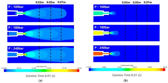
Figure 19.
Velocity and pressure contours in the x–axis direction at various pump pressures: (a) velocity contours; (b) pressure contours.
To validate the analysis results, we calculated the velocity at the nozzle tip by measuring the weight of a small tank filled with water before and after 10 s of water-jet spraying to determine the volumetric flow rate. Additionally, we generated an additional line probe at the nozzle tip in the CFD model to measure the average flow velocity ejected from the tip. By comparing the experimentally measured velocities at the nozzle tip with those obtained from the CFD analysis, we confirmed the consistency between the two methods. Table 6 presents the flow velocities at the nozzle tip for both the experimental measurements and the CFD analysis results. When examining the experimental value and the flow rate of the calculated value of the numerical analysis at the nozzle tip, the average flow rate error for each pressure was 5% or less, and a similar tendency was observed. Thus, the average flow velocity inside the nozzle was determined through CFD analysis.
Table 6.
Validity of numerical calculation.
The stagnation pressure () and wall shear stress (), which are the shear forces for removal, are calculated by numerically determining the average flow velocity () passing through the nozzle. For the measurement, a line probe (resolution: 20) was generated within the nozzle tube in the derived part of the analysis program. The flow velocities measured at each point were averaged to calculate the average flow velocity under each pressure condition. The calculated average flow velocity and Reynolds number within the nozzle tube are presented in Table 7.
Table 7.
Reynolds number and average flow velocity at each pressure.
4.3. Evaluation of the Bio-Fouling Cleaning Performance Effectiveness
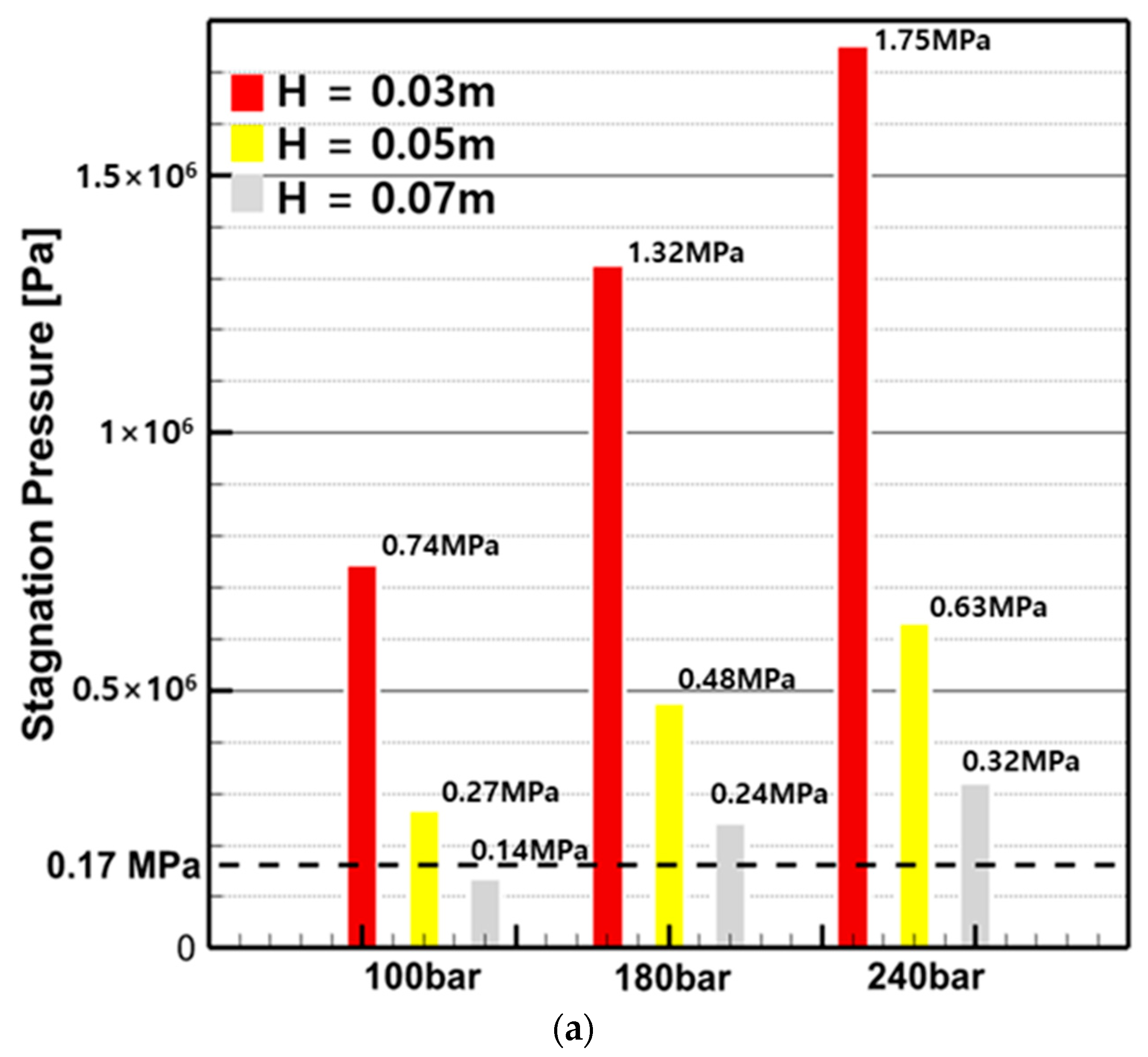
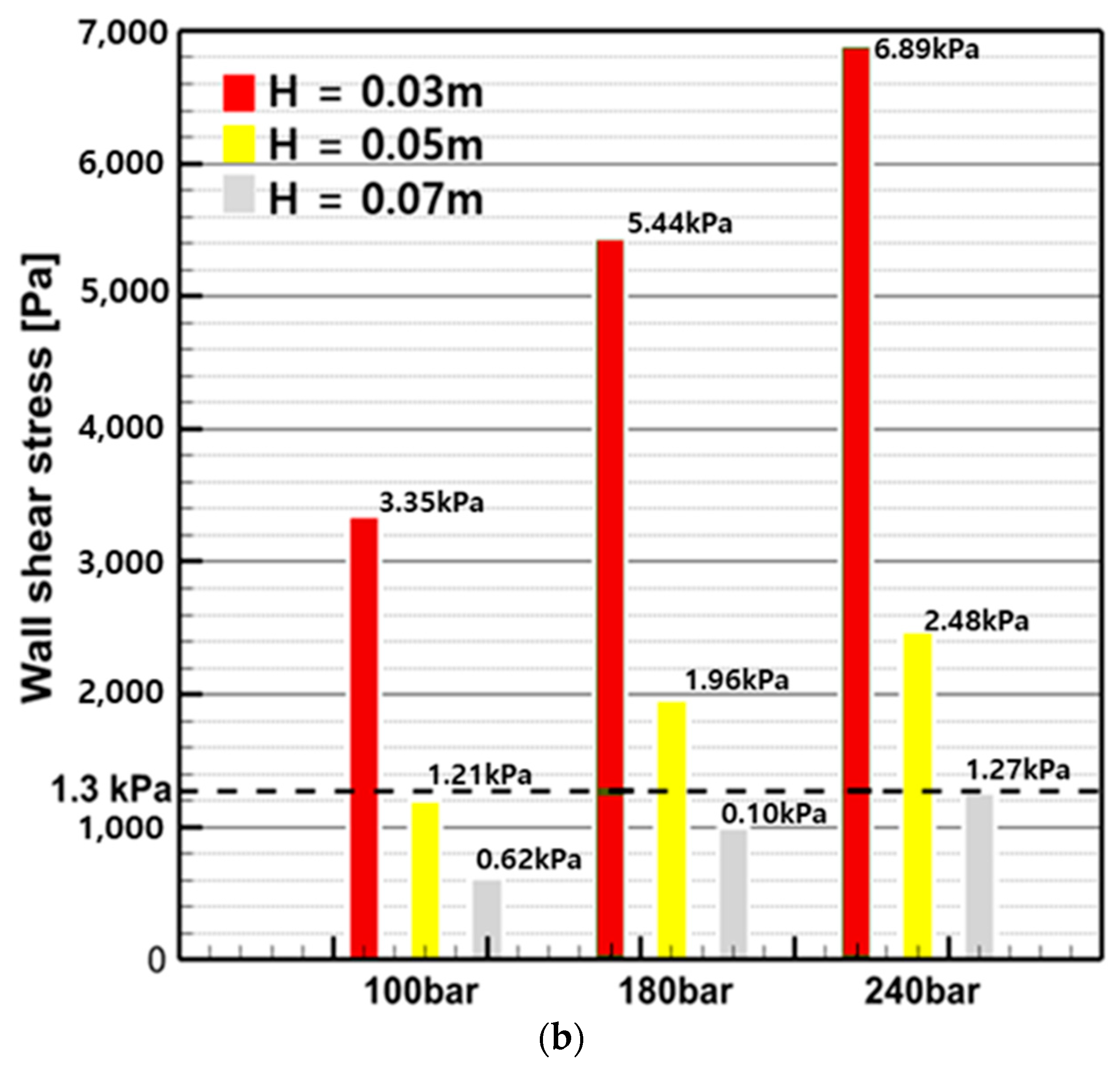
Figure 20 shows the stagnation pressure () and wall shear stress () calculated by substituting the average flow rate within the nozzle into Equations (4) and (5), based on pump pressure and spray distance. From the stagnation pressure results in Figure 20a, it can be observed that, except for the 100 bar, 0.07 m condition, all conditions have a pressure above 0.17 MPa, which is effective for removing micro-fouling. In the wall shear stress results of Figure 20b, when observing only H from the nozzle tip, the wall shear stress at 0.07 m did not meet the requirements for all pressures, and at 0.05 m, except for the 100 bar condition, all conditions had sufficient force to remove bio-fouling. At 0.03 m, all wall shear stress values were higher than the shear stress required for cleaning, indicating that effective cleaning is expected.


Figure 20.
Stagnation pressure and wall shear stress by pump pressure and spray distance: (a) stagnation pressure; (b) wall shear stress.
In summary, it was found that the closer the nozzle, the sufficient pressure and force transmission required for bio-fouling removal are ensured. The conditions that must be satisfied for stagnation pressure and wall shear stress are a minimum spray distance of 0.05 m and a minimum pump pressure of 180 bar. However, considering only the cleaning effect, the original stagnation pressure and wall shear stress calculation equations proposed by Oliveira and Granhag (2020) were designed with a focus on minimizing anti-fouling coating damage under biofilm and slime conditions [26]. As explained in Section 3, Figure 13 shows that minor damage appeared on the surface of the K1 specimen. Therefore, it is considered necessary to research the optimal conditions for each factor based on high-pressure water jets to prevent paint damage as well as to achieve cleaning effectiveness.
5. Evaluation of Cleaning Influence Factors through Image Analysis
Evaluating cleaning performance factors solely through visual inspection may have limitations in accurately assessing the removal effects. Therefore, to analyze the effects of the curing duration and various factors on the removal effectiveness post-experiment, the bio-fouling grades outlined in Table 1 were referenced. For this purpose, image analysis software was utilized. The specimens were divided into three areas for analysis, and image analysis was conducted with the assistance of the Korea Research Institute of Ships and Ocean Engineering (KRISO).
Table 8 shows the bio-fouling grade before and after the experiments for the specimens at different cultivation periods. For the ratings before the removal experiment, in the case of the Cu, K1, and K2 specimens, on day 42 for the Cu, K1, and K2 specimens, a rating of 2–3 was recorded, and this rating fluctuated around Grade 3 until the end of the experiment. In contrast, the HDPE specimen exhibited a rating of 5 on day 42 and maintained a rating above 5 from day 56 until the end of the experiment. This indicates that the growth rate of bio-foulings varies among the different specimen types. Examining the bio-fouling grades after the removal experiment, the Cu, K1, and K2 specimens consistently achieved Grades 0–1 across all cultivation periods, indicating a comprehensive removal effect regardless of the factor values. However, the HDPE specimens consistently recorded Grades 3–4 after the removal experiment for all cultivation periods, suggesting a lower removal effect compared to the other specimens because of the presence of large bio-foulings, such as barnacles. The reason the HDPE specimens did not reach Grade 1 after cleaning can be observed in the HDPE13 and HDPE14 specimens in Figure 13d. A pressure of 100 bar seems to have limitations for the removal of bio-foulings cultivated for approximately three months, and despite a pump pressure of 240 bar, large barnacles were attached, and widely distributed clusters of limpets remained on the surface. Barnacles are organisms that grow by attaching to algae and other substrates through a naturally adhesive byssus. Therefore, incomplete removal was presumably due to the presence of barnacles.
Table 8.
Extent of the fouling grade before and after bio-fouling removal experiment.
Image analysis was conducted to evaluate the factors influencing the cleaning performance of high-pressure water jet-based cleaning. An additional step involved separating the nine experimental conditions for each specimen subjected to the removal experiment into their respective factor values. The specimens selected for factor evaluation in the removal experiment were K1, K2, and Cu. Generally, owing to the presence of anti-fouling coatings on ship hulls and variations in the specimen height tolerance, we performed additional experiments on the W/O AF and HDPE specimens. These specimens had identical spray distances and towing carriage speed conditions. Notably, the HDPE specimen was excluded from the factor evaluation because it did not achieve Grade 1 after the experiment.
The number of Grade 1 achievements after the experiment, based on the factor values for each specimen, is summarized in Table 9, Table 10 and Table 11. Considering the pump pressure as the reference, the K1, K2, and Cu specimens achieved significantly more Grade 1 achievements at the maximum pump pressure of 240 bar compared to the other pressure conditions. Higher pressure levels seemed to have an effective removal effect, regardless of the size of the attached organisms. Regarding the spray distance criterion, a value of 0.03 m, representing a shorter distance between the nozzle and the specimen, would result in a higher number of Grade 1 achievements. However, except for the K2 specimen (0.03 m), a value of 0.05 m accounted for a higher proportion of Grade 1 achievements in the Cu and K1 specimens. These unexpected results could be attributed to the interaction between the size of the attached organism and the spray distance. For Grade 3 limpets, it was possible to achieve effective removal in narrow areas with high-speed delivery at shorter spray distances. However, for micro-fouling of Grade 2 or lower, even with a lower force, higher spray distances allow for cleaning over a wider area. Therefore, the factor values of 0.05 and 0.07 m resulted in a higher number of Grade 1 achievements. Regarding the towing carriage speed, except for the Cu specimen, there was no significant difference in the number of Grade 1 achievements among the factor values for specimens K1 and K2. Higher towing carriage speeds are effective in removing bio-foulings owing to the physical force of the impinging fluid, but the attachment strength varies depending on the size of the bio-foulings; therefore, micro-fouling with a weaker attachment strength can be removed even at lower speeds, leading to no noticeable differences among the factor values. Therefore, the towing carriage speed has relatively less influence on the cleaning performance of bio-fouling than pump pressure and spray distance.
Table 9.
Quantity of Grade 1 after cleaning for factors in K1 specimens.
Table 10.
Quantity of Grade 1 after cleaning for factors in K2 specimens.
Table 11.
Quantity of Grade 1 after cleaning for factors in Cu specimens.
The maximum and minimum Grade 1 achievement ratio differences among the factor values, which are associated with the cleaning performance, can be observed by examining the pump pressure and spray distance as factor values in the removal experiment. In terms of the pump pressure, K1, K2, and Cu had 51%, 69%, and 95% differences, respectively. For the spray distance, the differences were calculated to be 24% for K1, 32% for K2, and 50% for Cu. From the perspective of the removal experiment, the pump pressure is the dominant factor influencing the cleaning performance.
Additionally, for each material, the number of Grade 1 occurrences corresponding to the variations in the values of each factor was represented using box plots, as shown in Figure 21, to visually understand the distribution range of each factor. It is clearly observed that the distribution range of the number of Grade 1 occurrences for the pump pressure factor is wider than that of other factors across all specimen materials as the factor values change. Therefore, it can be concluded that pump pressure is the dominant factor affecting the cleaning performance. The next dominant factors are spray distance and towing carriage speed.
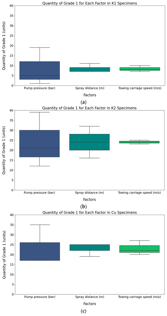
Figure 21.
Quantity of Grade 1 for each factor in specimens: (a) quantity of Grade 1 for K1; (b) quantity of Grade 1 for K2 specimens; (c) quantity of Grade 1 for Cu specimens.
6. Conclusions
This study has several limitations and assumptions, such as specimen damage and various error variables. Nevertheless, by conducting the cultivation process of bio-foulings on specimens and preparing for removal experiments, this research can serve as a reference for future similar experiments and is expected to be utilized as a foundational study for the development of hull-cleaning technologies based on high-pressure water-jet systems. In this study, the factors influencing cleaning performance were compared and validated through removal experiment results using high-pressure water-jet technology. Numerical calculations were performed to evaluate the cleaning performance of the nozzles used in the removal experiments and to estimate the stagnation pressure and wall shear stress required for the removal of hull-attached organisms. Additionally, specimens and experimental equipment were prepared to analyze the growth process of hull-attached organisms and the cleaning effects after removal. The conclusions drawn from the research process conducted as described above are as follows:
- (1)
- By employing the Taguchi method, an experimental design approach, and, assuming two repetitions of the experiments, nine experimental conditions were generated, as shown in Table 4. This approach allows for an effective analysis of the individual impact of each condition.
- (2)
- Through nozzle numerical analysis, it was confirmed that the conditions required to meet the stagnation pressure (~0.17 MPa) and wall shear stress (~1.3 kPa) necessary for the removal of bio-foulings are a minimum pump pressure of 180 bar and a minimum spray distance of 0.05 m. However, since the stagnation pressure and wall shear stress conditions are designed to minimize damage to anti-fouling coatings under biofilm and slime conditions, it is necessary to further find the optimal cleaning conditions that can prevent thickness damage as well as ensure cleaning effectiveness.
- (3)
- Image analysis of 168 test specimens cultivated in a marine environment for three months revealed that in the case of anti-fouling coatings and copper specimens, approximately Grade 2 coral-like formations were observed at the edges. In specimens without anti-fouling coatings and HDPE specimens, clusters of limpets, barnacles, and macro-fouling stages exceeding Grade 5 were observed.
- (4)
- After the removal experiment, image analysis revealed that the Grade 1 achievement rate of bio-fouling was the highest for pump pressure, showing a difference of 51% in K1, 69% in K2, and 95% in Cu compared to other factors. Additionally, by generating box plots to observe the distribution range of Grade 1 counts for each material, it was confirmed that the pump pressure factor exhibited a wider distribution range with changes in factor values compared to other factors. This indicates that pump pressure is the most dominant factor influencing hull-attached bio-fouling cleaning.
As part of our future, additional numerical calculations will be conducted by considering the nozzle movement speed to precisely evaluate the nozzle cleaning performance. Furthermore, based on the generated experimental conditions, measurements of the coating thickness before and after cleaning were performed, and the data were organized to determine the optimal conditions for bio-fouling removal while minimizing coating damage.
Author Contributions
Conceptualization, D.S., S.-g.C. and H.K.; methodology, K.Y. and J.A.; investigation, J.A. and S.A.B.; formal analysis, J.A.; software, J.A. and K.Y.; data curation, J.A., S.A.B. and J.O.; writing—original draft, J.A., S.A.B. and K.Y.; writing—review and editing, J.A., S.A.B. and J.O.; supervision, D.S., S.-g.C. and H.K.; funding acquisition, D.S., S.-g.C. and H.K. All authors have read and agreed to the published version of the manuscript.
Funding
This research was supported by Korea Institute of Marine Science & Technology Promotion (KIMST) funded by the Ministry of Oceans and Fisheries, Korea (RS-2023-00256122).
Institutional Review Board Statement
Not applicable.
Informed Consent Statement
Not applicable.
Data Availability Statement
The original contributions presented in the study are included in the article, further inquiries can be directed to the corresponding author/s.
Acknowledgments
This research was supported by the Korea Institute of Marine Science & Technology Promotion (KIMST) funded by the Ministry of Ocean and Fisheries, Korea (RS-2023-00256122). This research was also supported by the Korea Research Institute of Ships and Ocean Engineering and a grant from the Endowment Project of “Development of elemental technology and conceptual design for cleaning bio-fouling on niche area of international ship hull” funded by the Ministry of Oceans and Fisheries (1525013547).
Conflicts of Interest
The authors declare no conflicts of interest. The funders had no role in the design of the study, in the collection, analyses, or interpretation of data, in the writing of the manuscript, or in the decision to publish the results.
References
- International Maritime Organization. 2011 Guidelines for the Control and Management of Ships’ Biofouling to Minimize the Transfer of Invasive Aquatic Species; MEPC Resolution MEPC.207(62); IMO: London, UK, 2011. [Google Scholar]
- Cranfield, H.J.; Gordon, D.P.; Willan, R.C.; Marshall, B.A.; Battershill, C.N.; Francis, M.P.; Nelson, W.A.; Glasby, C.J.; Read, G.B. Adventive Marine Species in New Zealand; NIWA Technical Report 34; NIWA: Wellington, New Zealand, 1998; pp. 1–48. ISBN 0-478-08452-8. [Google Scholar]
- Hewitt, C.L.; Campbell, M.L.; Thresher, R.E.; Martin, R.B. (Eds.) Marine Biological Invasions of Port Phillip Bay, Victoria; Technical Report No. 20; CSIRO Division of Marine Research: Hobart, Australia, 1999; pp. 1–344. ISBN 0643062092. [Google Scholar]
- Park, J.K.; Hoe, C.H.; Kim, H.P.; Cho, Y.K. Study on the Biofouling Management of International Ships Entering South Korea. J. Korean Soc. Mar. Environ. Saf. 2022, 28, 10–18. [Google Scholar] [CrossRef]
- Hyun, B.; Shin, K.; Jang, M.-C.; Jang, P.-G.; Lee, W.-J.; Park, C.; Choi, K.-H. Potential invasions of phytoplankton in ship ballast water at South Korean ports. Mar. Freshw. Res. 2016, 67, 1906–1917. [Google Scholar] [CrossRef]
- Schultz, M.P. Effects of coating roughness and biofouling on ship resistance and powering. Biofouling 2007, 23, 331–341. [Google Scholar] [CrossRef]
- Champ, M.A. A review of organotin regulatory strategies, pending actions, related costs and benefits. Sci. Total Environ. 2000, 258, 21–71. [Google Scholar] [CrossRef] [PubMed]
- Ha, S.-Y.; Park, H.-S. A Case Study on the Management of Biofouling for Protection of the Marine Ecosystem. J. Navig. Port. Res. 2020, 44, 151–157. [Google Scholar] [CrossRef]
- Department of the Environment and New Zealand Ministry for Primary Industries. Anti-Fouling and In-Water Cleaning Guidelines; Commonwealth of Australia: Canberra, Australia, 2015; ISBN 978-1-76003-009-4. Available online: http://www.agriculture.gov.au/biosecurity/avm/vessels/biofouling/anti-fouling-and-inwater-cleaning-guidelines (accessed on 30 May 2022).
- Georgiades, E.; Growcott, A.; Kluza, D. Technical Guidance on Biofouling Management for Vessels Arriving to New Zealand; MPI Technical Paper No: 2018/07; Ministry for Primary Industries: Wellington, New Zealand, 2018; ISBN 978-1-77665-793-3. Available online: https://www.mpi.govt.nz/news-and-resources/publications/ (accessed on 23 May 2022).
- California State Lands Commission. Guidance Document for Biofouling Management Regulations to Minimize the Transfer of Nonindigenous Species from Vessels Arriving at California Ports; Marine Invasive Species Program: Sacramento, CA, USA, 2017. Available online: http://www.slc.ca.gov/Programs/MISP.html (accessed on 15 June 2022).
- Bohn, P.; Hansen, S.L.; Møller, J.K.; Stuer-Lauridsen, F. Non-Indigenous Species from Hull Fouling in Danish Marine Waters; The Danish Nature Agency: Copenhagen, Denmark, 2016; ISBN 978-87-7175-558-9.
- Hyun, B.; Jang, P.-G.; Shin, K.; Kang, J.-H.; Jang, M.-C. Ship’s Hull Fouling Management and In-Water Cleaning Techniques. J. Korean Soc. Mar. Environ. Saf. 2018, 24, 785–795. [Google Scholar] [CrossRef]
- Woods, C.; Floerl, O.; Fitridge, I.; Johnston, O.; Robinson, K.; Rupp, D.; Davey, N.; Rush, N.; Smith, M. Efficacy of Hull Cleaning Operations in Containing Biological Material: II. Seasonal Variability; MAF Biosecurity New Zealand Technical Paper Series 08/11; The National Institute of Water and Atmospheric Research Ltd.: Wellington, New Zealand, 2007; ISBN 978-0-478-32191-3. [Google Scholar]
- Park, S.J.; Choi, S.M.; Kim, D.G. Study on the Policy for the Preemptive Response to the Biofouling; Korea Maritime Institute: Busan, Republic of Korea, 2020; pp. 1–148. [Google Scholar]
- Suk, J.-H. A Study on the Regulatory Framework Related to Ship’s Biofouling. Korean Marit. Law. Assoc. 2018, 30, 139–167. [Google Scholar] [CrossRef]
- Floerl, O.; Inglis, G.J.; Hayden, B.J. A Risk-Based Predictive Tool to Prevent Accidental Introductions of Nonindigenous Marine Species. Environ. Manag. 2005, 35, 765–778. [Google Scholar] [CrossRef] [PubMed]
- Davidson, I.; Floerl, O.; Fletcher, L.; Cahill, P. Level of Fouling Rank Scale—An Updated Guideline; Prepared for Auckland Council: Auckland, New Zealand, 2019; pp. 1–14.
- Bixler, G.D.; Bhushan, B. Biofouling: Lessons from Nature. Phil. Trans. R. Soc. A 2012, 370, 2381–2417. [Google Scholar] [CrossRef]
- Moser, C.S.; Wier, T.P.; First, M.R.; Grant, J.F.; Riley, S.C.; Robbins-Wamsley, S.H.; Tamburri, M.N.; Ruiz, G.M.; Miller, A.W.; Drake, L.A. Quantifying the extent of niche areas in the global fleet of commercial ships: The potential for ‘‘super-hot spots’’ of biofouling. Biol. Invasions 2017, 19, 1745–1761. [Google Scholar] [CrossRef]
- Cohen, A.N.; Zabin, C.J.; Ashton, G.V.; Brown, C.W.; Brousseau, D.J.; David, A.A.; Davidson, I.C.; de Rivera, C.E.; Draheim, R.; Geller, J.; et al. SLC Biofouling Condition and Parasites 2013 FINAL Report. 2013.
- Hua, J.; Chiu, Y.-S.; Tsai, C.-Y. En-route operated hydroblasting system for counteracting biofouling on ship hull. Ocean. Eng. 2018, 152, 249–256. [Google Scholar] [CrossRef]
- Song, C.; Cui, W. Review of Underwater Ship Hull Cleaning Technologies. J. Mar. Sci. Appl. 2020, 19, 123–136. [Google Scholar] [CrossRef]
- Bertram, V. Robotic Hull Cleaning—Past, Present and Prospects. In Proceedings of the 20th International Conference on Computer and IT Applications in the Maritime Industries (COMPIT ’21), Mülheim, Germany, 9–10 August 2021; Hamburg University of Technology: Hamburg, Germany, 2021; pp. 16–23, ISBN 978-3-89220-724-5. [Google Scholar]
- Oliveira, D.R.; Larsson, L.; Granhag, L. Towards an Absolute Scale for Adhesion Strength of Ship Hull Microfouling. Biofouling 2019, 35, 244–258. [Google Scholar] [CrossRef] [PubMed]
- Oliveira, D.R.; Granhag, L. Ship Hull In-Water Cleaning and Its Effects on Fouling-Control Coatings. Biofouling 2020, 36, 332–350. [Google Scholar] [CrossRef] [PubMed]
- Seo, D.; Oh, J. Experimental Study on the Removal of Biofouling from Specimens of Small Ship Constructions Using Water Jet. J. Korean Soc. Mar. Environ. Saf. 2022, 28, 1078–1085. [Google Scholar] [CrossRef]
- Lim, P.; Yang, G.-E. Optimal Cutting Condition of Tool Life in the High Speed Machining by Taguchi Design of Experiments. J. Korean Soc. Manuf. Process Eng. 2006, 5, 59–64. [Google Scholar]
- Park, C.S.; Jung, Y.J. A Case Study for Resolution of Variation and Determination of Optimum Conditions in Taguchi’s Design of Experiments. J. Korean Math. 2002, 9, 45–74. [Google Scholar]
- Grzegorczyk, M.; Pogorzelski, S.J.; Pospiech, A.; Boniewicz-Szmyt, K. Monitoring of Marine Biofilm Formation Dynamics at Submerged Solid Surfaces with Multitechnique Sensors. Front. Mar. Sci. 2018, 5, 363. [Google Scholar] [CrossRef]
- Hayek, M.; Salgues, M.; Souche, J.-C.; Cunge, E.; Giraudel, C.; Paireau, O. Influence of the Intrinsic Characteristics of Cementitious Materials on Biofouling in the Marine Environment. Sustainability 2021, 13, 2625. [Google Scholar] [CrossRef]
- Woods Hole Oceanographic Institute. Marine Fouling and Its Prevention; Contribution No., 580; U.S. Naval Institute: Annapolis, MD, USA; George Banta Publishing Co.: Menasha, WI, USA, 1952. [Google Scholar]
- Hearin, J.; Hunsucker, K.Z.; Swain, G.; Stephens, A.; Gardner, H.; Lieberman, K.; Harper, M. Analysis of Long-Term Mechanical Grooming on Large-Scale Test Panels Coated with an Antifouling and a Fouling-Release Coating. Biofouling 2015, 31, 625–638. [Google Scholar] [CrossRef]
- Ningegowda, B.M.; Rahantamialisoa, F.N.Z.; Zembi, J.; Pandal, A.; Im, H.G.; Battistoni, M. Large Eddy Simulations of Supercritical and Transcritical Jet Flows using Real Fluid Thermophysical Properties. In Proceedings of the SAE World Congress, Detroit, MI, USA, 21–23 April 2020. [Google Scholar] [CrossRef]
- Xiao, F.; Wang, Z.G.; Sun, M.B.; Liang, J.H.; Liu, N. Large Eddy Simulation of Liquid Jet Primary Breakup in Supersonic Air Crossflow. Int. J. Multiph. Flow 2016, 87, 229–240. [Google Scholar] [CrossRef]
- Gohil, T.B.; Saha, A.K.; Muralidhar, K. Large Eddy Simulation of a Free Circular Jet. J. Fluids Eng. 2014, 136, 051205. [Google Scholar] [CrossRef]
- Menter, F.; Hüppe, A.; Matyushenko, A.; Kolmogorov, D. An Overview of Hybrid RANS–LES Models Developed for Industrial CFD. Appl. Sci. 2021, 11, 2459. [Google Scholar] [CrossRef]
- Lopes, D.; Puga, H.; Teixeira, J.; Lima, R.; Grilo, J.; Dueñas-Pamplona, J.; Ferrera, C. Comparison of RANS and LES Turbulent Flow Models in a Real Stenosis. Int. J. Heat. Fluid. Flow. 2024, 107, 109340. [Google Scholar] [CrossRef]
- Yang, Y.; Li, W.; Shi, W.; Zhang, W.; El-Emam, M.A. Numerical Investigation of a High-Pressure Submerged Jet Using a Cavitation Model Considering Effects of Shear Stress. Processes 2019, 7, 541. [Google Scholar] [CrossRef]


Disclaimer/Publisher’s Note: The statements, opinions and data contained in all publications are solely those of the individual author(s) and contributor(s) and not of MDPI and/or the editor(s). MDPI and/or the editor(s) disclaim responsibility for any injury to people or property resulting from any ideas, methods, instructions or products referred to in the content. |
© 2024 by the authors. Licensee MDPI, Basel, Switzerland. This article is an open access article distributed under the terms and conditions of the Creative Commons Attribution (CC BY) license (https://creativecommons.org/licenses/by/4.0/).