Abstract
The real-time classification of fish feeding behavior plays a crucial role in aquaculture, which is closely related to feeding cost and environmental preservation. In this paper, a Fish Feeding Intensity classification model based on the improved Vision Transformer (CFFI-Vit) is proposed, which is capable of quantifying the feeding behaviors of rainbow trout (Oncorhynchus mykiss) into three intensities: strong, moderate, and weak. The process is outlined as follows: firstly, we obtained 2685 raw feeding images of rainbow trout from recorded videos and classified them into three categories: strong, moderate, and weak. Secondly, the number of transformer encoder blocks in the internal structure of the ViT was reduced from 12 to 4, which can greatly reduce the computational load of the model, facilitating its deployment on mobile devices. And finally, a residual module was added to the head of the ViT, enhancing the model’s ability to extract features. The proposed CFFI-Vit has a computational load of 5.81 G (Giga) Floating Point Operations per Second (FLOPs). Compared to the original ViT model, it reduces computational demands by 65.54% and improves classification accuracy on the validation set by 5.4 percentage points. On the test set, the model achieves precision, recall, and F1 score of 93.47%, 93.44%, and 93.42%, respectively. Additionally, compared to state-of-the-art models such as ResNet34, MobileNetv2, VGG16, and GoogLeNet, the CFFI-Vit model’s classification accuracy is higher by 6.87, 8.43, 7.03, and 5.65 percentage points, respectively. Therefore, the proposed CFFI-Vit can achieve higher classification accuracy while significantly reducing computational demands. This provides a foundation for deploying lightweight deep network models on edge devices with limited hardware capabilities.
1. Introduction
The feeding of fish plays a crucial role in recirculating aquaculture systems [1] as it directly impacts production efficiency and costs [2]. In practical production, feeding is mainly carried out through manual assessment and mechanical feeding, which cannot meet the actual needs of fish, resulting in overfeeding or underfeeding [3]. Overfeeding not only leads to feed wastage but also pollutes the water environment and increases the risk of fish disease [4]. Underfeeding can lead to slow fish growth, which affects economic profitability [5]. Quantitative analysis of fish feeding behavior intensity can directly reflect fish appetite. Therefore, identifying fish feeding behavior not only helps aquaculture farmers reduce breeding costs but also protects the environment [6].
There are various methods for quantifying fish feeding behavior, including machine vision [7,8], acoustic sensors [9,10], water quality sensors [11], and other sensors [12]. Compared to machine vision, methods such as acoustic and water quality sensors can only indirectly assess fish feeding intensity by measuring factors such as uneaten feed or water quality [13,14,15]. Acoustic sensors are primarily used for detecting the distribution of fish schools [16]. Therefore, in quantifying fish feeding intensity, machine vision provides a more direct approach [17]. Machine vision can quantify fish feeding intensity by capturing images of fish feeding using visual sensors, extracting features from the images [7,18] and analyzing them directly. To improve the feeding quality of Tilapia, Ye et al. [19] first extracted the behavioral characteristics of fish schools (speed and turning angle) using optical flow. Then, they estimated the feeding intensity of the fish based on statistical imaging techniques. Subsequently, Zhao et al. [8] further derived a novel modified kinetic energy model for predicting fish hunger status, based on the premise of extracting the spatial dispersion degree of shoal. Zhou et al. [20] utilized Delaunay Triangulation to extract the positional information of each fish within the school, thereby quantifying the feeding intensity of fish. In their research, the team also employed a neuro-fuzzy model for analyzing fish feeding behavior and established an adaptive network-based fuzzy inference system (ANFIS) [21]. Razman, Susto, Cenedese, Majeed, Musa, Ghani, Adnan, Ismail, Taha and Mukai [7] initially employed Principal Component Analysis to reduce the dimensionality of high-dimensional features. Subsequently, Support Vector Machine (SVM), k-Nearest Neighbor (k-NN), and Random Forest Tree models were used individually to differentiate hunger levels of Lates calcarifer in an automated feeding system. The aforementioned methods mentioned for quantifying fish feeding intensity all require manual feature extraction before utilizing model classification. Manual feature extraction introduces subjectivity, and the accuracy of the experimental results depends on the quality of the extracted features [22]. Therefore, this can lead to inaccurate quantification results.
On the other hand, deep learning does not require manual feature extraction [23,24], which reduces subjectivity in the analysis and quantification process [25]. Currently, the main deep neural network models used for fish feeding classification are based on Convolutional Neural Networks (CNNs) as the backbone network [26,27]. In research on detecting and evaluating fish appetite, Zhou et al. [28] initially augmented their collected data using techniques such as rotation, scaling, and noise invariance. Subsequently, the LeNet5 CNN was employed to quantitatively classify fish feeding intensity. Måløy et al. [29] designed a Dual-Stream Recurrent Network (DSRN), taking both temporal and spatial factors into account. This neural network comprises a spatial network, a 3D convolutional motion network, and an LSTM recurrent classification network. The model predicts salmon feeding behavior with an accuracy of 80%. Ubina et al. [30] presented a deep optical flow neural network based on a 3D Convolutional Neural Network (3D CNN) to predict fish feeding intensity. First, the two consecutive images in a video were passed through an optical flow neural network to generate intermediate frames, which were then fed into an I3D dual-stream network [31] to evaluate fish feeding behavior, achieving an accuracy of 95%. Zhang et al. [6] proposed a method based on MobileNetV2 and SENet for identifying fish school feeding behavior. By preprocessing images with operations such as random cropping and brightness-contrast adjustment, and utilizing a feature weighting network, they achieved an identification accuracy of 97.76%. Compared to models based on EfficientNet_B0, ShuffleNetV2, AlexNet, and EfficientNetV2, their method showed significant improvements, demonstrating its effectiveness in real aquaculture environments. Feng et al. [32] developed a lightweight 3D ResNet-GloRe network for the real-time quantification of fish feeding intensity, achieving 92.68% accuracy. Their method reduced model parameters by 46.08% and GFLOPs by 44.10%, outperforming the classical 3D ResNet by 4.88% in accuracy. In addition to the methods mentioned above for directly quantifying fish feeding behavior through fish feeding videos or images, researchers have also analyzed fish feeding behavior intensity indirectly by obtaining videos of bait remaining in the water [33]. The aforementioned studies are all based on convolutional neural networks, which utilize convolutional kernels to extract image features. Convolutional neural networks are limited to extracting local features, whereas self-attention networks can extract global features [34]. Self-attention networks were initially applied in the field of machine translation [35]. In machine translation tasks, the input is a sentence, and the output is the corresponding translated sentence. In traditional sequence-to-sequence models, recurrent neural networks (RNNs) [36] or long short-term memory networks (LSTMs) [37] are commonly used to process input sequences, but these models suffer from limitations such as finite memory length and poor parallelism. The introduction of self-attention mechanisms changed this situation. Self-attention mechanisms allow the model to dynamically allocate attention weights when processing input sequences, enabling better capture of dependencies between different positions in the sentence [34]. This attention mechanism enables the model to consider information from all positions in the input sentence simultaneously, thereby improving the performance of the model. Combining convolutional networks with attention mechanisms [34] for image classification has also become a growing trend in the field. Yang, et al. [38] considered spatial relationships and designed a network model consisting of two parallel attention modules [39], based on the EfficientNet-B2 architecture, to quantify fish feeding behavior. They employed training techniques such as the Mish activation function, Ranger optimizer, label smoothing, etc., to improve model accuracy. Their model outperforms classic CNN models such as AlexNet [40], VGG16 [41], GoogLeNet [42], DenseNet [43], and ResNet [44] in terms of accuracy and precision. Moreover, their model has fewer parameters and less computational complexity compared to the aforementioned classic CNN networks.
Currently, in research on quantifying fish feeding classification, models primarily utilize a CNN as the backbone network. However, traditional CNNs extract features layer by layer through a local receptive field, which limits their ability to capture global information in the initial layers. A broader understanding of the global context usually requires deeper network architectures or specially designed modules. In deep networks, gradients may become very small (vanish) or very large (explode) during the backpropagation process, making the network difficult to train. Vanishing gradients can lead to slow learning or complete stagnation in the training process, while exploding gradients may cause numerical issues during training. As the depth of the network increases, adjusting parameters becomes more challenging, leading to instability and suboptimal training outcomes. Even with advanced optimization algorithms, without additional aids such as residual connections [44], deep networks are difficult to converge. The residual network (ResNet), proposed by Kaiming He [44], is a deep neural network architecture aimed at addressing the issues of vanishing and exploding gradients during the training of deep networks. In recent years, the Vision Transformer has drawn inspiration from the successful application of the Transformer model in the field of natural language processing (NLP) [45]. In NLP, the Transformer model is widely used to process sequence data, such as text sequences [46]. ViT adopts the self-attention mechanism of the Transformer to handle image data. It divides the image into individual image patches and then converts these image patches into sequential data, which are input into the Transformer model for processing. By modeling the relationships between image patches, the ViT model captures global information, enabling it to consider the overall structure and context of the image, not just local features. However, ViT requires substantial computational resources from hardware and needs a large amount of data for training. The multilayer stacking of the transformer encoder within its internal structure accounts for most of the model’s computational demands. Reducing the number of these stacks can significantly decrease the computational requirements of the model.
In this context, we propose a novel Fish Feeding Intensity classification model based on the improved Vision Transformer, named CFFI-Vit, designed to quantify the feeding behaviors of rainbow trout (Oncorhynchus mykiss). The key contributions of this research are outlined as follows:
- A Vision Transformer (ViT) model was initially trained on the ImageNet_21K dataset and used as the backbone of the proposed model, with the number of encoder blocks significantly reduced. This modification significantly decreases the computational load, making the model more efficient and suitable for deployment on edge devices.
- To further improve the model’s performance, a residual module was incorporated into the head of the ViT. This addition enhances the model’s ability to extract intricate features from the input data, thereby improving classification accuracy.
- The CFFI-Vit model was rigorously tested, significantly reducing the computational load while improving the accuracy of classifying rainbow trout feeding intensity into strong, moderate, and weak categories. It can accurately classify fish feeding behaviors.
To advance the field of aquaculture, the proposed model effectively balances efficiency and accuracy, making it highly suitable for real-time deployment in aquaculture environments. This fills existing research gaps and supports better management and optimization of feeding practices. The structure of the remainder of this paper is as follows. Section 2 describes the experiments and methods, Section 3 presents the results and analysis, and Section 4 concludes the findings.
2. Materials and Methods
2.1. Materials
The experiment used rainbow trout procured from the Shuntong Breeding Base in Huairou District, Beijing, China. Each fish had an average weight of 500 ± 10 g, with a total of 120 individuals. As fish are sensitive organisms and can react strongly to changes in their environment, all fish were acclimatized to the experimental conditions for one and a half months upon arrival to minimize the impact of stress reactions on the experimental results. This experiment was conducted at the Aquatic Precision Aquaculture Laboratory of the Information Technology Research Center, Beijing Academy of Agriculture and Forestry Sciences. The experimental environment consisted of a recirculating aquaculture system (RAS), as shown in Figure 1, comprising a total of 6 fish tanks (each tank has a diameter of approximately 1 m and a depth of 1.2 m), with 20 fish placed in each tank. The dissolved oxygen concentration in the water was maintained at 9–12 mg/L, and the water temperature was 16 ± 0.5 °C. Following the commencement of the experiment, manual feeding of fish in each tank occurred daily at 9 a.m. and 6 p.m. The feed provided to the fish contained essential nutrients: a minimum of 52% crude protein, at least 11% crude fat, a maximum of 5% crude fiber, and up to 13% crude ash (Hanye Biotechnology Co., Ltd., Rizhao, China). The feeding amount was generally around 1.6% of the fish’s body weight. Video data collection was conducted using a GoPro Hero8 (14 mm focal length). To mitigate the effects of surface reflections during data acquisition, the camera angle was set at a 45-degree angle relative to the water surface (Figure 1).
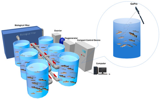
Figure 1.
The structure of the experimental system.
2.2. Establishment of the Dataset
In this experiment, the feeding intensity of rainbow trout is classified into 3 categories: strong, moderate, and weak (Figure 2), as shown in Table 1. Previous studies classified fish feeding intensity into four levels: strong, moderate, weak, and none [9,47]. Considering the practical scenario in aquaculture where machine vision devices halt feeding when detecting weak feeding intensity, the “none” feeding intensity was not included in this experiment. The dataset processing procedure is outlined as follows: The fish feeding videos start recording 10 s before feeding begins and stop 10 s after the fish finish feeding and become calm. This ensures that the entire feeding cycle of the fish is captured. The video clips were captured at a frame rate of 60 Hz and a resolution of 1920 × 1080 pixels. The data collection spanned over 2 months, resulting in a total of 120 video segments, each lasting 28–32 s (Table 2). To reduce data similarity, 3600 images were extracted by sampling 2 frames per second from the videos. From these, 2685 images were selected, with 1710 images used as the training and validation sets and the remaining 975 images used as the test set (Table 3). The detailed breakdown of data obtained for each category is shown in Table 1. The images were manually annotated and classified into three levels of feeding intensity: strong, moderate, and weak. The ground truth of the images was established by the experimental team members over a period of two weeks. The classification was based on prior classifications and the team’s expertise [9]. The accuracy of the classification was ensured through thorough cross-verification and consensus among the team members. The images used for training and validation underwent data augmentation techniques such as flipping, translation, and noise addition, resulting in a final dataset of 6919 images, with 5536 images allocated for training and 1383 images allocated for validation. The classification and sample numbers of the dataset are shown in Table 3.
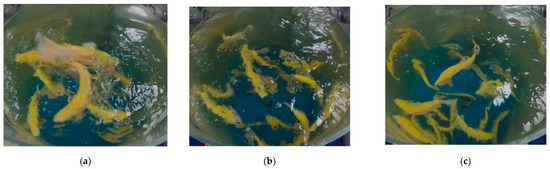
Figure 2.
Classification of feeding intensity at three levels. (a) Strong. (b) Moderate. (c) Weak.

Table 1.
Three-level feeding intensity classification.
Table 2.
Detailed breakdown of fish feeding classification data.
Table 3.
The classification and sample numbers of the dataset.
2.3. The Proposed Model Architecture
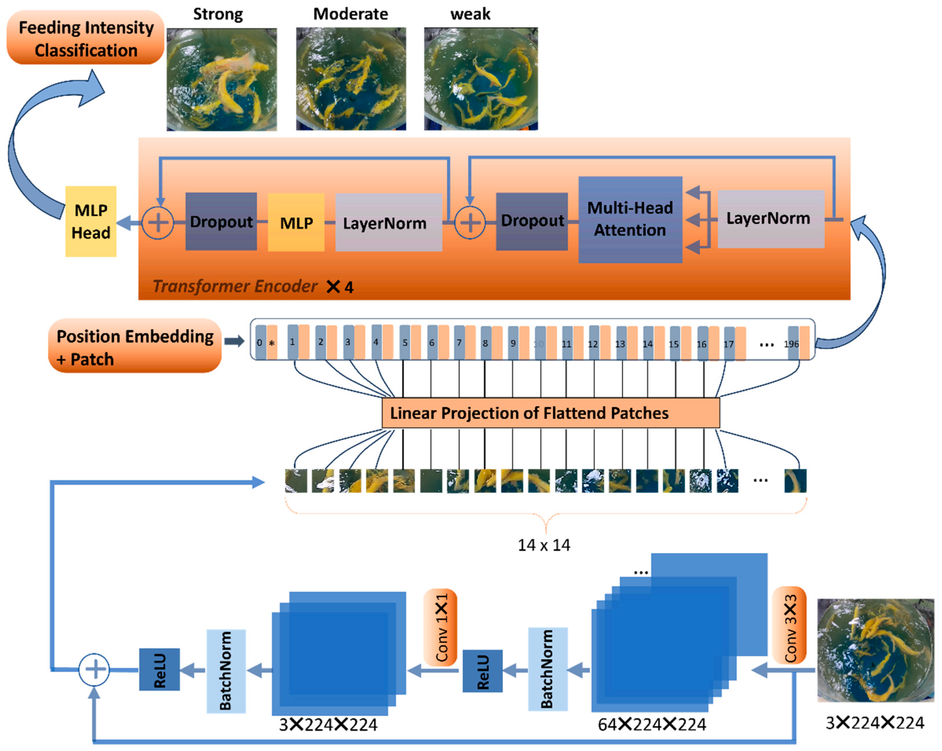
The new model combining ViT with the residual structure is illustrated in Figure 3. The pretrained weights of the ViT-B/16_21K model are used to train the new model. This model is a ViT Base-class benchmark model with a patch size of 16 and was trained on the ImageNet-21K datasets. First, before being segmented into patches by the ViT model, the input image undergoes feature extraction through a residual module. Subsequently, the image, after feature extraction, is segmented into patches and then flattened. Next, all of the flattened patches, along with position encoding, are fed into the modified transformer encoder. Finally, the classification results are output through a Multilayer Perceptron head. The specific modules are as follows in sequence.
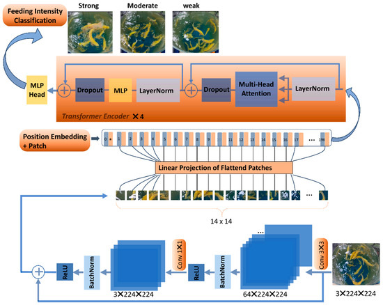
Figure 3.
The structure of the proposed CFFI-Vit model.
2.3.1. Residual Module
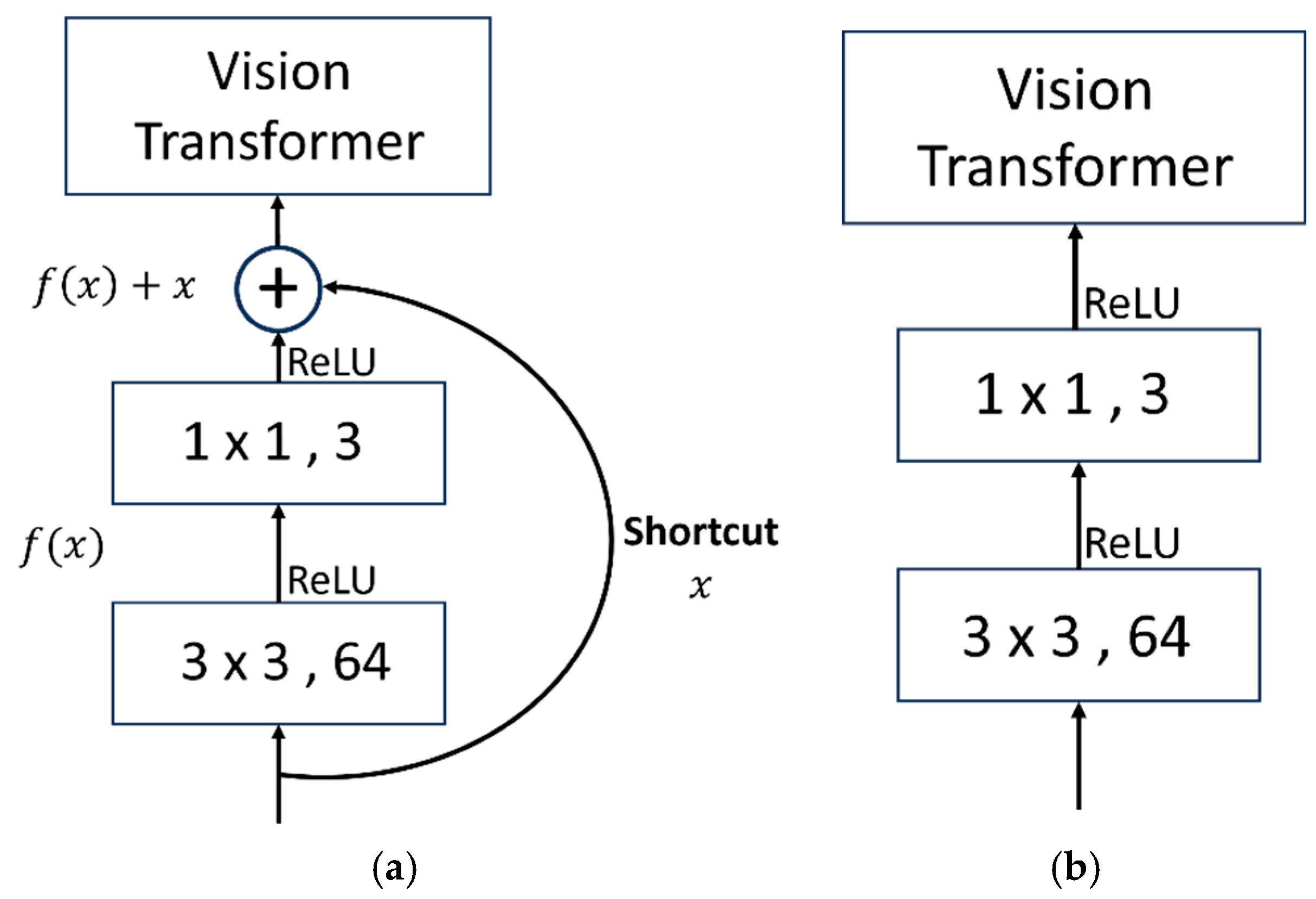
Before processing the image into patches, a residual module was introduced for feature extraction. The residual network (ResNet) is a deep neural network architecture that introduces skip connections between layers to address the problems of vanishing and exploding gradients during training. It was proposed by researchers at Microsoft Research Asia and has achieved great success in the ImageNet large-scale image recognition field. The ResNet module typically consists of several residual blocks. Each residual block contains two branches: a main branch and a skip connection (shortcut) branch (Figure 4a). The main branch typically consists of a series of convolutional layers and activation functions, while the skip connection branch directly passes the input signal to the output, allowing the network to learn residuals rather than directly learning feature mappings. The computational formula is represented as follows, as shown in Equation (1). Among them, denotes the result obtained by processing the input data through convolutional layers and activation functions ReLU [48], and represents the original input data. The addition of the two yields the final output . This design effectively alleviates the problem of gradient vanishing, enabling the network to be trained deeper and more easily. In addition to using the residual structure, it was also compared with regular convolutional modules (plain convolution network), as shown in Figure 4b.
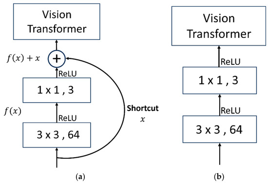
Figure 4.
Residual network module and plain network schematic diagram. (a) Residual network. (b) Plain network.
2.3.2. Patch Embedding Layer
The inspiration behind Vision Transformer stems from the Transformer [34] architecture’s success in NLP tasks, particularly in capturing long-range dependencies and contextual information from sequences of tokens. Unlike CNNs, which rely on local receptive fields and hierarchical feature extraction. Transformers employ self-attention mechanisms [34] to attend to all tokens in the input sequence simultaneously, enabling efficient modeling of global dependencies. In Vision Transformer, the handling of image blocks (patches) is similar to the handling of tokens in NLP. Therefore, after linear embedding, they are also referred to as patch tokens. It consists of several key components, including the Patch Embedding layer, the Transformer Encoder, the Multi-Head Attention mechanism, the Multilayer Perceptron (MLP) layer, the Layer Normalization layer, and the classification head.
When the input image undergoes feature extraction by the preceding residual module, it is then divided into many small patches of size 3 × 224 × 224. Due to each containing patches of size 16 × 16, a photo with three-channel data is divided into (224/16)2 = 196 tokens. As shown in Figure 3, tokens 0–196 correspond to vectors, with each token having a dimension of 768 (16 × 16 × 3). Additionally, a position encoding of dimension (1, 768) is added on top of each token with the same dimension as the token. Positional encoding is added to the token embeddings to incorporate spatial information. Before inputting into the Transformer Encoder, a classification token needs to be added. This “class” token is a trainable parameter with the same dimension as the other tokens, which is 768. It is concatenated with the tokens previously generated from the image to form a two-dimensional vector of dimension (197, 768). These token embeddings are then processed by a stack of Transformer Encoders.
2.3.3. Transformer Encoder Structure
The number of Transformer Encoders in the proposed model is 4. It includes the LayerNorm layer, Multi-Head Attention (MHA) layer, Dropout/DropPath layer (in this case, Dropout is used), and MLP layer. After the input embedded patches go through Layer Normalization and Multi-Head Attention mechanism processing, they are then added with the original input embedded patch data through residual connection, as shown in Equation (2). represents the output of the th layer, which is the feature representation after processing by the current layer. represents the output of the ()th layer, i.e., the feature representation from the previous layer. L represents the total number of layers in the Transformer Encoder. Then, they go through the LayerNorm layer and MLP layer sequentially. The resulting data are added to the previous data in Equation (3), where the MLP contains two non-linear GELU layers.
- (1)
- LayerNorm
The LayerNorm layer standardizes the input to ensure that each feature dimension has a comparable scale and distribution. This normalization assists in training and the network’s convergence by minimizing the effect of internal covariate shifts. Its formula is represented as Equation (4). represents the input embedded token vector, which is the data to be normalized. and are learnable parameters, known as the scale factor and bias term, respectively. They are used to adjust the scale and offset of the normalized data, making the normalized data more suitable for network training. represents the mean of the input along each feature dimension. represents the standard deviation of the input along each feature dimension. is a very small number, typically set to 10−5 by default. Its purpose is to prevent the denominator from being zero. LayerNorm normalizes the values of each feature dimension in each sample, ensuring that their mean is 0 and standard deviation is 1. By carrying out normalization, it reduces the likelihood of gradient explosion or vanishing during training, thus enhancing the stability and training speed of the network.
- (2)
- Multi-Head Attention
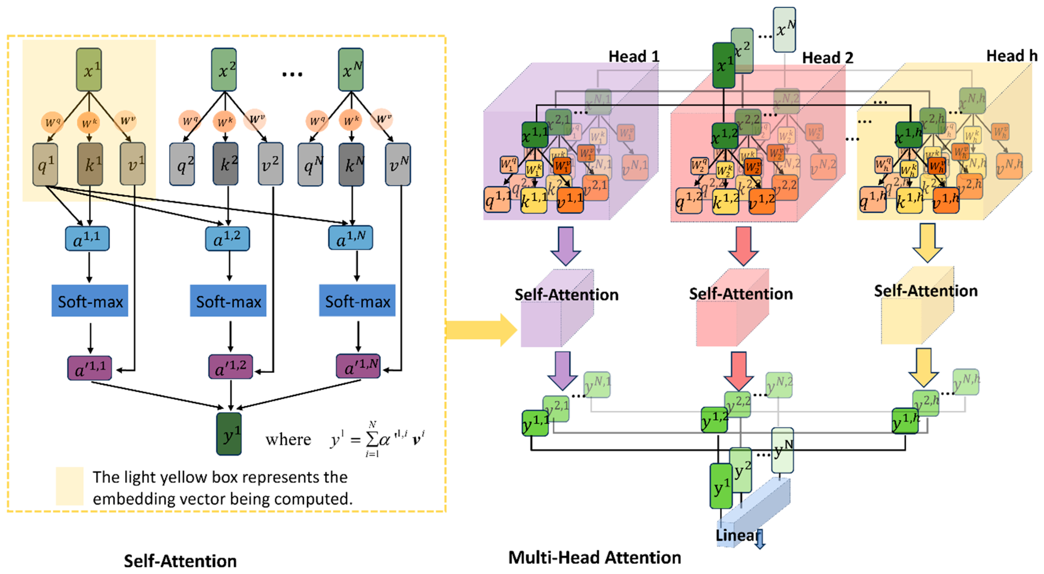
The Multi-Head Attention (MHA) mechanism is derived from the Self-Attention structure, and the two mechanisms are shown in Figure 5. Self-Attention allows each element in the input sequence to interact with all other elements in the sequence. In Equation (5), Q, K and V represent sets of q, k, and v, respectively, where Q stands for query, K stands for key, and V represents the information extracted from . For each image sequence input data (, , … ) with a length of N, N is 197. After input embedding, each sequence x is flattened into a one-dimensional vector of size (768). Subsequently, these 197 sequences are individually multiplied by three weight matrices , , and (which are trainable and shared) to obtain corresponding , , and (). Then, each in the sequence is multiplied by each transposed in the sequence and divided by a scaling factor , where represents the length of each sequence, which is 768 in this case. The results obtained from the above operation are then processed through softmax activation and finally weighted and cumulatively summed with each in the sequence, according to Equation (6). Multi-Head Attention operates by running multiple Self-Attention layers in parallel and synthesizing their results. After the sequence embedding data are input, each sequence is divided into parts, that is, for heads, the number of in each base model is 12, while in each large model, there are 16 heads. Each ‘head’ independently learns different attention weights as in Equation (7), where . Then, the outputs of these self-attention layers (12) for each sequence are combined, concatenated (Equation (8), ) and then passed through a linear layer, which is further processed in the subsequent neural network layer. In this way, Multi-Head Attention enables the model to capture information from different subspaces of the input sequence simultaneously, thereby enhancing the model’s expressive power.

Figure 5.
Self-Attention and Multi-Head Attention module structure.
- (3)
- Dropout Layer
Dropout layer is a regularization technique used during neural network training to randomly set a portion of neuron outputs to zero. By randomly deactivating some neurons, Dropout prevents excessive interdependence between neurons in the network, thereby avoiding the phenomenon of neuron co-adaptation. Therefore, it can reduce network complexity, thus reducing the risk of overfitting, and improve the model’s generalization ability and robustness.
- (4)
- MLP Block
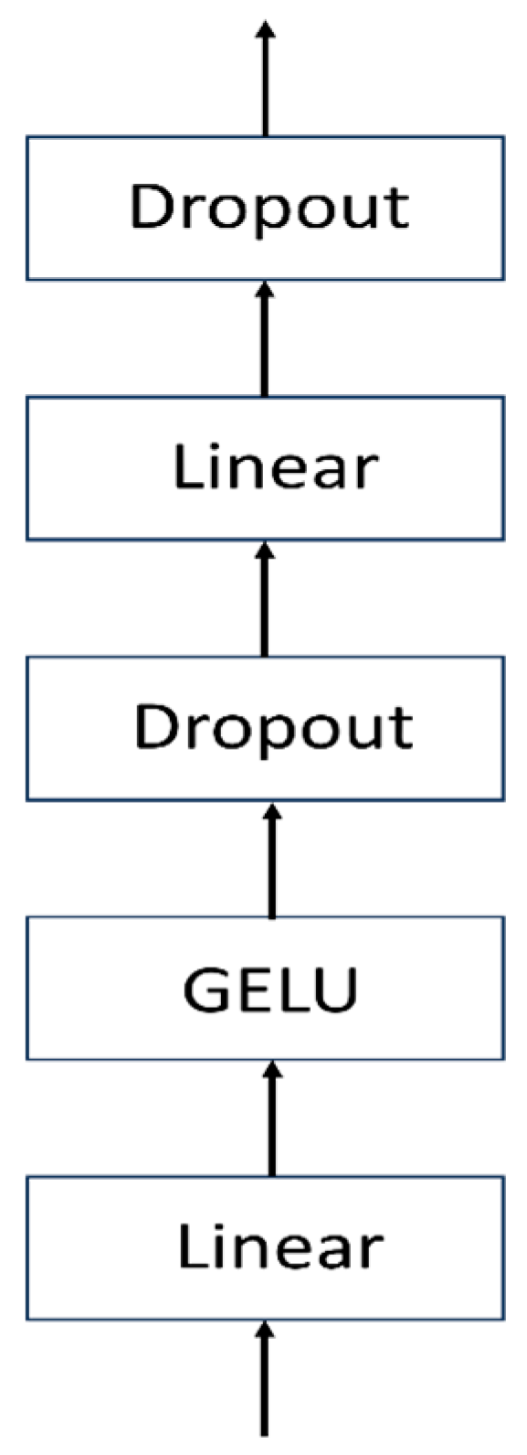
The MLP Block consists of two linear fully connected layers, one GELU activation layer, and two Dropout layers (Figure 6). The first linear layer increases the dimensionality, followed by a GELU activation and then a Dropout layer to regularize the data. Next, the data pass through another linear layer, which restores the dimensionality to that before the first linear layer. Finally, it passes through another Dropout layer before outputting.

Figure 6.
MLP Block flowchart.
2.3.4. MLP Head
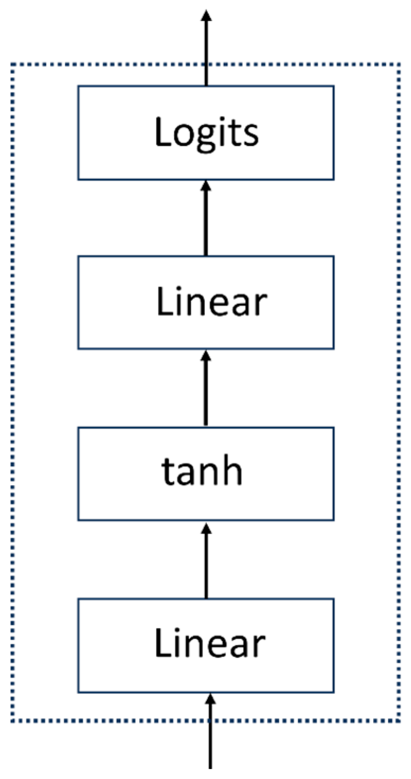
The MLP Head serves as the final layer of the Vision Transformer model, responsible for further nonlinear transformations and feature extraction on the encoded features from the encoder blocks to obtain the ultimate classification results. The MLP Head consists of linear fully connected layers and activation functions. It consists of Linear + tanh activation function + Linear layers (Figure 7).
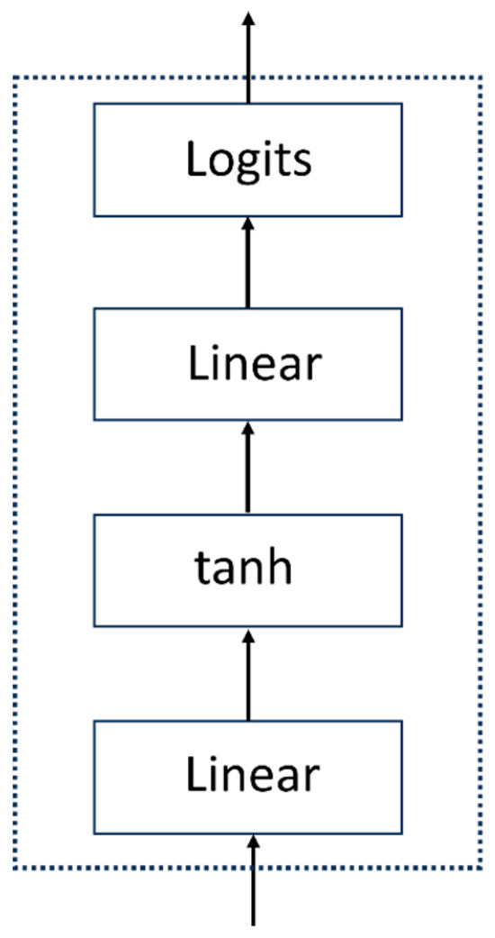
Figure 7.
Flowchart of the MLP Head module.
2.4. Performance Evaluation Indexes
In this study, precision, recall, F1 score, and accuracy were adopted as the evaluation metrics for the proposed models. Their calculation formulas are shown respectively in Equations (9)–(12). TP (True Positives) refer to the instances where the model accurately recognizes positive class samples as positive. FP (False Positives), also termed “false alarms”, happen when the model mistakenly classifies negative class samples as positive. TN (True Negatives) represent the cases where the model correctly identifies negative class samples as negative. FN (False Negatives) are the instances where the model incorrectly identifies positive class samples as negative. Precision is the ratio of true positive predictions to the total number of samples predicted as positive. Recall is the ratio of true positive predictions to the total number of actual positive samples, reflecting the model’s capability to detect positive samples. The F1 score, which is the harmonic mean of precision and recall, provides a balanced measure of the model’s precision and recall performance. The value of this parameter falls within the range of 0~1, and a higher F1 score indicates better performance of the model. Accuracy is the proportion of correctly classified samples among all samples.
3. Results and Discussion
In this experiment, the CFFI-Vit model used transfer learning [49] to classify the feeding intensity of rainbow trout. In our experiments, we used the Adam optimizer [50] with the initial learning rate set to 0.001. The total number of epochs was 300, and the batch size was set to 32. To dynamically adjust the learning rate, we employed the StepLR scheduler. Specifically, the learning rate is multiplied by 0.5 every 30 epochs. This strategy helps the model gradually converge during training and helps prevent oscillations caused by a learning rate that is too high. The hyperparameter information is shown in Table 4. In addition, we compared the model with the state-of-the-art classification models ViT, ResNet34, MobileNetv2, VGG16, and GoogLeNet.
Table 4.
Hyperparameter information.
The software and hardware information used for the experiments is listed in Table 5, and the detailed model layer structure information is listed in Table 6.
Table 5.
Experimental hardware and software configuration.
Table 6.
Detailed model layer structure information.
3.1. Experimental Results of the Proposed Model
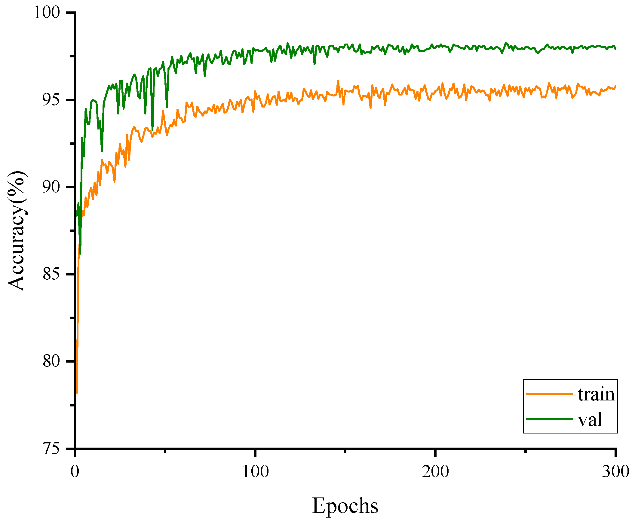
The accuracy results on the training set and the validation set for the CFFI-Vit are presented in Figure 8. The graph shows that the accuracy on the validation set remains higher than that on the training set after approximately 10 epochs, indicating that the accuracy of fish feeding intensity classification is better on the validation set than on the training set. The initial classification accuracy on the training set is 78.2%, and both the training and validation accuracies exhibit fluctuating upward trends during the first 100 epochs. After 100 epochs, the accuracies of both the training set and validation set gradually stabilize. Training set accuracy converges around 95.79%, while validation set accuracy converges at 98.63%.
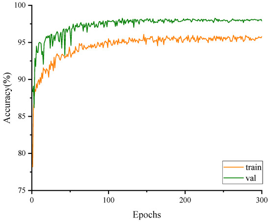
Figure 8.
Training and validation results of the model.
For the accuracy of the results, we performed a 10-fold cross-validation on the training and validation datasets. The validation results are shown in Table 7.
Table 7.
Ten-fold cross-validation results.
The data in the table demonstrate the robustness and consistency of our model. The average training loss is 0.102 with a standard deviation of 0.01, and the average training accuracy is 96.11% with a standard deviation of 0.32%. The average validation loss is 0.05 with a standard deviation of 0.015, and the average validation accuracy is 98.31% with a standard deviation of 0.61%. These results indicate that our model performs consistently across different folds, with high accuracy and low variability.
3.2. Performance Metrics of the Models on the Test Set
When analyzing the performance of the proposed model on the test set, it was compared with other three similarly processed ViT models. The other three models are ViT-B/16+Res, ViT-L/16+Res, and ViT-L/16_21K+Res. The structural similarities and differences of the four models are presented in Table 8. ViT-B/16 refers to the Base-class pretrained model, which possesses 12 Multi-Head Attention (MHA) units and a patch size of 16 and was trained on the ImageNet-1K datasets. In contrast, ViT-L/16 and ViT-L/16_21K represent the Large-class pretrained models, each equipped with 16 Multi-Head Attention (MHA) units and a patch size of 16, trained on the ImageNet-1K and ImageNet-21K datasets, respectively.
Table 8.
The similarities and differences of the four models.
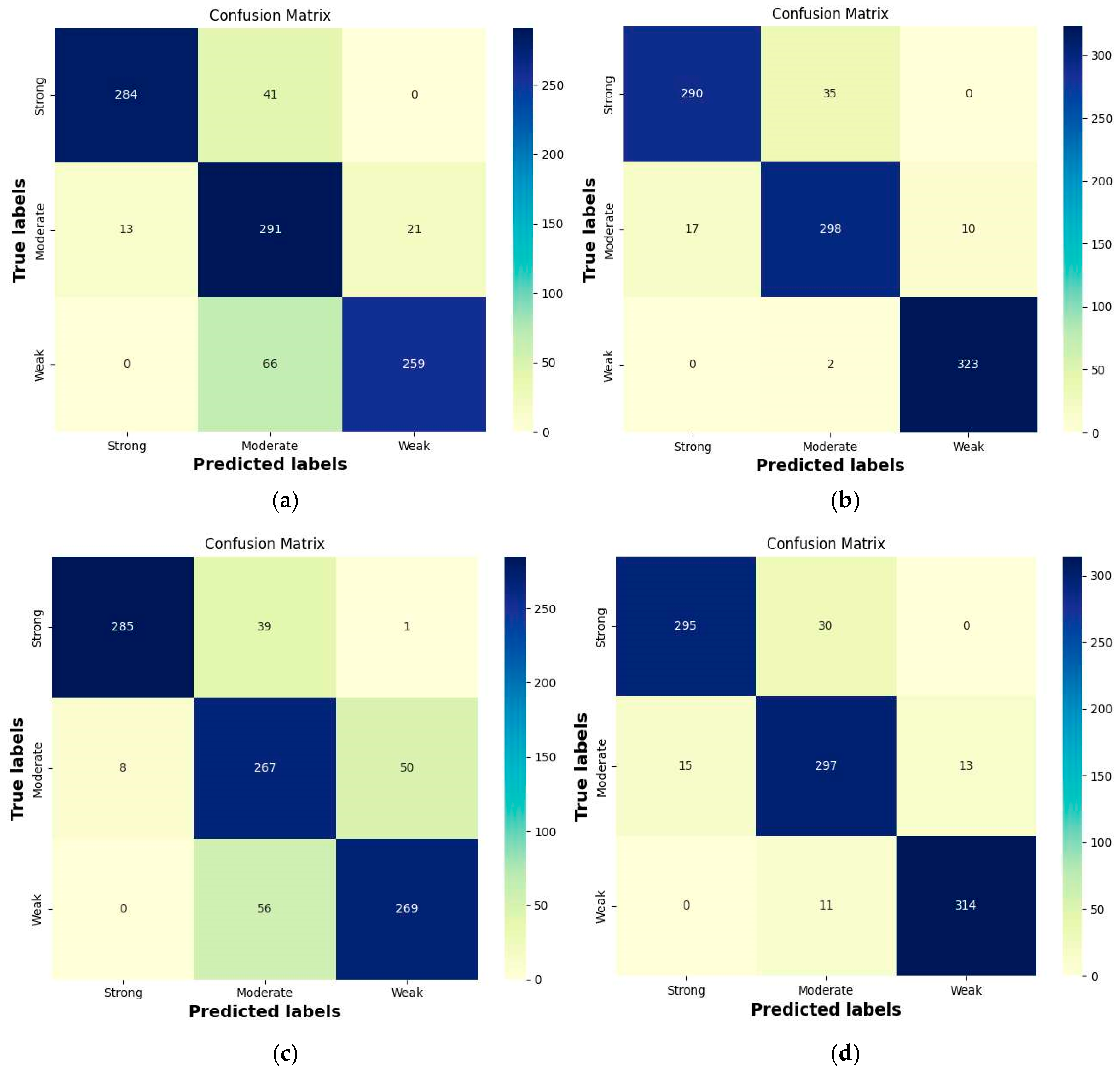
The confusion matrix results of the four models and example predictions on the test set for the three-class classification are shown in Figure 9 and Figure 10, respectively. From Figure 9, we can see that the four models have an average misclassification rate of 11.15% for “strong” feeding behavior as “moderate”. The number of misclassifications is 41, 35, 39, and 30, respectively. However, except for ViT-L/16+Res, which misclassified one “strong” feeding intensity instance as “weak”, the other three models did not misclassify “strong” feeding intensity as “weak”. This is because “strong” feeding intensity sometimes appears visually similar to “moderate” intensity (Figure 10b), leading to misclassification by the models, whereas the visual difference between “strong” and “weak” intensity is more significant, resulting in accurate classification (Figure 10c). When predicting “moderate” feeding intensity, ViT-B/16+Res and ViT-L/16+Res are more likely to incorrectly predict it as “weak,” as shown in Figure 10f. In contrast, ViT-B/16-21K+Res and ViT-L/16-21K+Res tend to misclassify “moderate” feeding intensity as “strong” rather than “weak” more often, possibly because these two models extract features that bias toward the “strong” category (Figure 10d). When predicting the third class of feeding intensity, “weak,” the number of times they incorrectly classify it as “moderate” is 66, 2, 56, and 11, respectively. It is evident that ViT-B/16-21K+Res and ViT-L/16-21K+Res perform significantly better in this category compared to ViT-B/16+Res and ViT-L/16+Res, especially our proposed model, ViT-B/16-21K+Res, which only misclassifies “weak” as “moderate” in 2 instances (Figure 10h). Overall, models pretrained on the ImageNet-21K dataset and adapted through transfer learning perform better in the tri-classification of fish feeding intensities than those trained on the ImageNet-1K dataset, particularly in reducing the number of misclassifications of “weak” as “moderate.” This may be attributed to the former models’ superior feature extraction capabilities and their ability to discern subtle differences between different feeding intensities. The other four performance metrics, precision, recall, F1 score, and accuracy, are shown in Table 9. From the table, it is evident that our model performs optimally across various metrics.

Figure 9.
Confusion matrices of the proposed models on the test set. (a) ViT-B/16+Res. (b) ViT-B/16+Res_21K. (c) ViT-L/16+Res. (d) ViT-L/16+Res_21K.
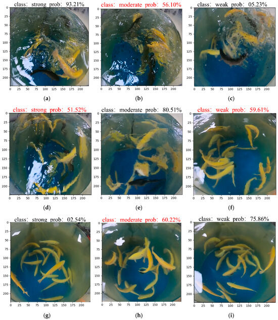
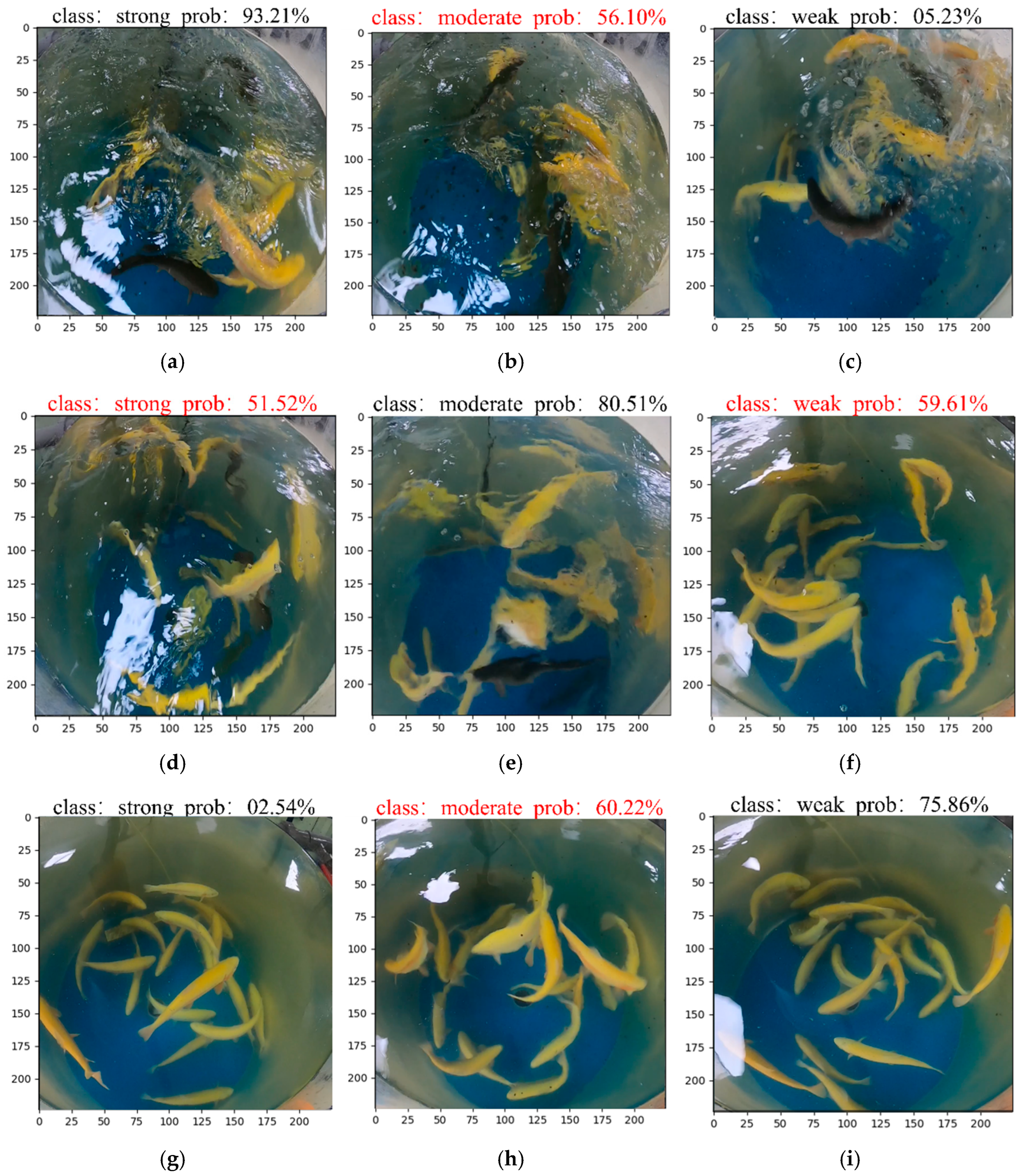
Figure 10.
Classification prediction matrix on the test set. Red font displays classification errors. (a) “strong” feeding intensity predicted as “strong”. (b) “strong” feeding intensity misclassified as “moderate”. (c) “strong” feeding intensity not misclassified as “weak”. (d) “moderate” feeding intensity misclassified as “strong”. (e) “moderate” feeding intensity predicted as “moderate”. (f) “moderate” feeding intensity misclassified as “weak”. (g) “weak” feeding intensity not misclassified as “strong”. (h) “weak” feeding intensity misclassified as “moderate”. (i) “weak” feeding intensity predicted as “weak”.
Table 9.
The performance metrics of the four models.
3.3. Ablation Experiments
In this experiment, ablation studies were conducted on the proposed model. The ViT base model was first tested for classification accuracy of feeding intensity with only four internal transformer encoders. Subsequently, the impact of adding convolutional layers and residual structures was evaluated, as detailed in Table 10.
Table 10.
Model ablation experiment.
The results indicate that the model enhanced with CNN and particularly ResNet structures exhibited significant improvements in accuracy. This demonstrates that integrating traditional CNN frameworks and residual network structures is highly effective in boosting the performance of ViT models. In the modifications based on the ViT-B/16_21K as the baseline model, the number of transformer encoders in its structure was first set to 4, which is denoted as ViT(4) in Table 10. On this basis, a convolutional head and a residual head were subsequently added to the model, respectively, and we observed their classification accuracies. According to the table, the classification accuracy of ViT(4) on the validation set is 90.46%. After adding a convolutional head (ViT(4)+CNN), the accuracy increases to 95.73%, which is an increase of 5.27 percentage points. The accuracy of ViT(4)+Res is the highest at 98.63%, which is 2.9 percentage points higher than ViT(4)+CNN and 8.17 percentage points higher than ViT(4).
Despite the increased complexity and accuracy of the proposed model, the rise in FLOPs was minimal, highlighting the efficiency of our model design. These ablation experiments reveal that the inclusion of CNN and ResNet structures within ViT models can effectively enhance performance while maintaining reasonable computational costs. This strategy provides valuable insights for the design of deep learning models, especially for tasks requiring high accuracy and computational efficiency.
This paper also explores the impact of different numbers of transformer encoder blocks in ViT on the classification accuracy of feeding intensity after incorporating the same residual blocks. As shown in Table 11, ViT+Res (4), the proposed model, has 4 transformer encoder blocks. It was compared with models that have 8, 12, 16, 20, and 24 transformer encoder blocks. According to the table, the highest classification accuracy on the validation set, at 99.13%, is achieved when the number of transformer encoder blocks is 12. Compared to ViT+Res (4), the accuracy is only increased by 0.50 percentage points, but the computational load and parameter count increase by 192.08% and 191.94%, respectively. Therefore, the proposed model can significantly reduce computational requirements without compromising accuracy.
Table 11.
Comparison of accuracy with different transformer encoders.
Additionally, classification accuracy was also determined by adding different residual modules, while keeping the number of transformer encoders in the ViT fixed at 4. The residual modules were inspired by ResNet34 [44], with their network structure shown in Table 12. The first three stages of ResNet34 were chosen and modified to add to the front of the modified ViT. The filters in Stage 2 of ResNet34 were set to 16, 32, 64, and 128, and the filters in Stage 3 were set to 3 to match the input channels of the subsequent ViT. The accuracy and model parameters of all combinations on the validation set are shown in Table 13.
Table 12.
The network structure of ResNet34.
Table 13.
Comparison of accuracy with different combinations of residual structures.
From Table 13, it can be seen that among the combinations of {16, 3}, {32, 3}, and {64, 3}, the classification accuracy on the validation set gradually increases, reaching the highest value at 91.32% in the {64, 3} combination. However, when the number of convolution kernels increases to 128, the classification accuracy begins to decrease. This indicates that classification accuracy does not necessarily improve with an increase in the number of convolution kernels in the residual structure.
3.4. Comparison with State-of-the-Art Models
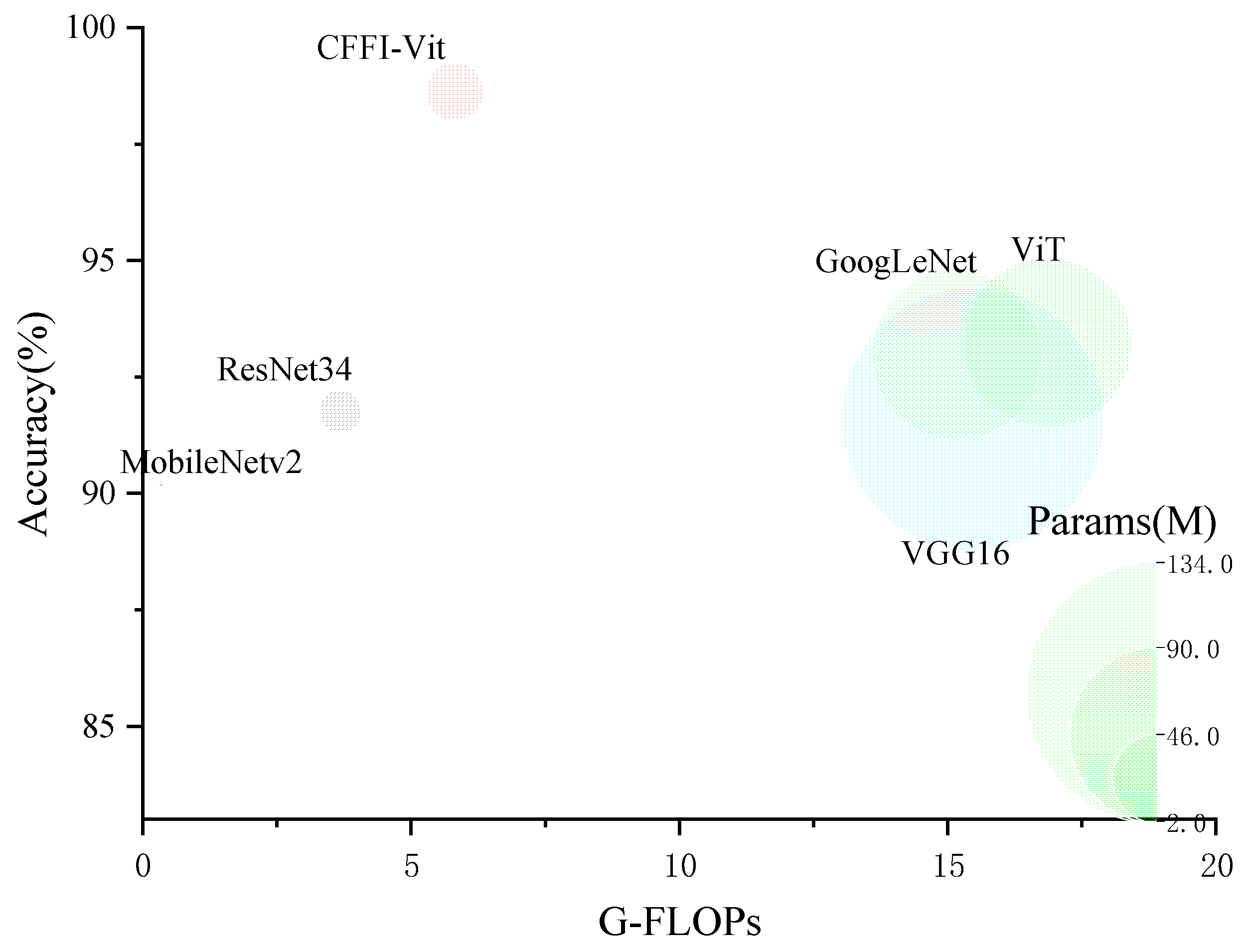
To verify the superiority of the proposed model in classification accuracy, it was compared with the original ViT model, ResNet34, MobileNetv2, VGG16, and GoogLeNet. An intuitive graph of their classification accuracies on the validation set, along with the computational demands and parameter sizes of each model, is presented in Figure 11, with specific data detailed in Table 14.
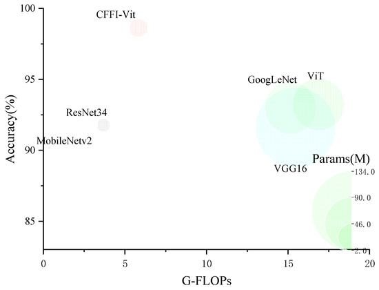
Figure 11.
Model attribute comparison chart.
Table 14.
Comparison of accuracy and model properties.
From Figure 11, it is evident that the proposed network model, CFFI-Vit, significantly outperforms the other models in terms of classification accuracy on the validation set. It also has a considerably smaller parameter size compared to the original ViT model, VGG16, and GoogLeNet. According to Table 14, although the proposed model has a slightly higher number of model parameters and higher computational requirements than ResNet34, it achieves a classification accuracy that is higher by 6.87 percentage points. Compared to MobileNetv2, although it has 27.31 M fewer parameters than CFFI-Vit, the accuracy of MobileNetv2 is 8.43 percentage points lower. When compared with VGG16, GoogLeNet, and the original ViT model, the proposed model’s computational demands are 68.91%, 61.70%, and 65.54% lower, respectively, and its classification accuracies are 7.03, 5.65, and 5.4 percentage points higher, respectively. This demonstrates that the proposed model not only optimizes computational efficiency but also significantly enhances the classification accuracy of fish feeding intensity.
4. Conclusions
In this paper, a modified new model based on the ViT base model, named CFFI-Vit, was used to identify the three-class feeding intensity of rainbow trout. Setting the transformer encoder module to 4 can significantly reduce the computational load compared to the original ViT model. Additionally, the inclusion of residual modules enhances feature extraction, thereby improving the model’s classification accuracy. The proposed model achieved a classification accuracy of 98.63% on the validation set. Compared to the original ViT model, it reduces the computational demand by 65.54% and increases the classification accuracy of fish feeding intensity on the validation set by 5.4 percentage points. Performance evaluation metrics from the modified model on the test set indicated that its classification accuracy of fish feeding was lower than that on the validation set, suggesting the need for larger training datasets in future experiments. Additionally, we explored adding different residual structures before the ViT model patches. The results demonstrated that increasing the number of convolutional kernels in the residual layers did not improve classification accuracy but rather led to a decrease.
In summary, the experimental results validate the feasibility and effectiveness of the proposed models in classifying fish feeding intensity, opening new possibilities for the application of deep learning models in biological research and providing valuable insights for future related studies. Of course, there are also some limitations. Future research will incorporate multi-modal studies by combining information from audio, water quality sensors, and other sources.
Author Contributions
Conceptualization, J.L. and C.Z.; funding acquisition, C.Z.; methodology, J.L., A.T.B. and J.F.B.-B.; project administration, X.Y.; resources, X.Y.; software, Z.Z.; supervision, J.F.B.-B.; visualization, A.T.B.; writing—original draft, J.L.; writing—review and editing, Z.Z. and C.Z. All authors have read and agreed to the published version of the manuscript.
Funding
This work was supported by the National Natural Science Foundation of China (32373184) and the National Key Research and Development Program of China (2022YFD2001701).
Institutional Review Board Statement
Not applicable.
Informed Consent Statement
Not applicable.
Data Availability Statement
The datasets created and/or analyzed during the current study are available from the corresponding author upon reasonable request.
Conflicts of Interest
The authors declare no conflicts of interest.
References
- Afewerki, S.; Asche, F.; Misund, B.; Thorvaldsen, T.; Tveteras, R. Innovation in the Norwegian aquaculture industry. Rev. Aquac. 2023, 15, 759–771. [Google Scholar] [CrossRef]
- Mandal, A.; Ghosh, A.R. Role of artificial intelligence (AI) in fish growth and health status monitoring: A review on sustainable aquaculture. Aquac. Int. 2024, 32, 2791–2820. [Google Scholar] [CrossRef]
- AlZubi, H.S.; Al-Nuaimy, W.; Buckley, J.; Young, I. An intelligent behavior-based fish feeding system. In Proceedings of the 2016 13th International Multi-Conference on Systems, Signals & Devices (SSD), Leipzig, Germany, 21–24 March 2016; pp. 22–29. [Google Scholar]
- Buerger, A.N.; Parente, C.E.; Harris, J.P.; Watts, E.G.; Wormington, A.M.; Bisesi, J.H., Jr. Impacts of diethylhexyl phthalate and overfeeding on physical fitness and lipid mobilization in Danio rerio (zebrafish). Chemosphere 2022, 295, 133703. [Google Scholar] [CrossRef] [PubMed]
- Chen, L.; Yang, X.; Sun, C.; Wang, Y.; Xu, D.; Zhou, C. Feed intake prediction model for group fish using the MEA-BP neural network in intensive aquaculture. Inf. Process. Agric. 2020, 7, 261–271. [Google Scholar] [CrossRef]
- Zhang, L.; Wang, J.; Li, B.; Liu, Y.; Zhang, H.; Duan, Q. A MobileNetV2-SENet-based method for identifying fish school feeding behavior. Aquac. Eng. 2022, 99, 102288. [Google Scholar] [CrossRef]
- Razman, M.A.M.; Susto, G.A.; Cenedese, A.; Majeed, A.P.A.; Musa, R.M.; Ghani, A.S.A.; Adnan, F.A.; Ismail, K.M.; Taha, Z.; Mukai, Y. Hunger classification of Lates calcarifer by means of an automated feeder and image processing. Comput. Electron. Agric. 2019, 163, 104883. [Google Scholar] [CrossRef]
- Zhao, J.; Gu, Z.; Shi, M.; Lu, H.; Li, J.; Shen, M.; Ye, Z.; Zhu, S. Spatial behavioral characteristics and statistics-based kinetic energy modeling in special behaviors detection of a shoal of fish in a recirculating aquaculture system. Comput. Electron. Agric. 2016, 127, 271–280. [Google Scholar] [CrossRef]
- Zeng, Y.; Yang, X.; Pan, L.; Zhu, W.; Wang, D.; Zhao, Z.; Liu, J.; Sun, C.; Zhou, C. Fish school feeding behavior quantification using acoustic signal and improved Swin Transformer. Comput. Electron. Agric. 2023, 204, 107580. [Google Scholar] [CrossRef]
- Iqbal, U.; Li, D.; Du, Z.; Akhter, M.; Mushtaq, Z.; Qureshi, M.F.; Rehman, H.A.U. Augmenting Aquaculture Efficiency through Involutional Neural Networks and Self-Attention for Oplegnathus Punctatus Feeding Intensity Classification from Log Mel Spectrograms. Animals 2024, 14, 1690. [Google Scholar] [CrossRef]
- Wu, T.-H.; Huang, Y.-I.; Chen, J.-M. Development of an adaptive neural-based fuzzy inference system for feeding decision-making assessment in silver perch (Bidyanus bidyanus) culture. Aquac. Eng. 2015, 66, 41–51. [Google Scholar] [CrossRef]
- Mukai, Y.; Taha, Z.; Ismail, K.M.; Tan, N.H.; Mohd Razman, M.A.; Mat Jizat, J.A. High growth rates of Asian seabass (Lates calcarifer Bloch, 1790) fry reared using a demand feeder with an image processing system for detecting fish behaviour. Aquac. Res. 2021, 52, 5093–5098. [Google Scholar] [CrossRef]
- Liu, J.; Bienvenido, F.; Yang, X.; Zhao, Z.; Feng, S.; Zhou, C. Nonintrusive and automatic quantitative analysis methods for fish behaviour in aquaculture. Aquac. Res. 2022, 53, 2985–3000. [Google Scholar] [CrossRef]
- Llorens, S.; Pérez-Arjona, I.; Soliveres, E.; Espinosa, V. Detection and target strength measurements of uneaten feed pellets with a single beam echosounder. Aquac. Eng. 2017, 78, 216–220. [Google Scholar] [CrossRef]
- Chu, D. Technology evolution and advances in fisheries acoustics. J. Mar. Sci. Technol. 2011, 19, 2. [Google Scholar] [CrossRef]
- Trygonis, V.; Georgakarakos, S.; Dagorn, L.; Brehmer, P. Spatiotemporal distribution of fish schools around drifting fish aggregating devices. Fish. Res. 2016, 177, 39–49. [Google Scholar] [CrossRef]
- Zhang, L.; Li, B.; Sun, X.; Hong, Q.; Duan, Q. Intelligent fish feeding based on machine vision: A review. Biosyst. Eng. 2023, 231, 133–164. [Google Scholar] [CrossRef]
- Li, D.; Wang, Q.; Li, X.; Niu, M.; Wang, H.; Liu, C. Recent advances of machine vision technology in fish classification. ICES J. Mar. Sci. 2022, 79, 263–284. [Google Scholar] [CrossRef]
- Ye, Z.; Zhao, J.; Han, Z.; Zhu, S.; Li, J.; Lu, H.; Ruan, Y. Behavioral characteristics and statistics-based imaging techniques in the assessment and optimization of tilapia feeding in a recirculating aquaculture system. Trans. ASABE 2016, 59, 345–355. [Google Scholar]
- Zhou, C.; Zhang, B.; Lin, K.; Xu, D.; Chen, C.; Yang, X.; Sun, C. Near-infrared imaging to quantify the feeding behavior of fish in aquaculture. Comput. Electron. Agric. 2017, 135, 233–241. [Google Scholar] [CrossRef]
- Zhou, C.; Lin, K.; Xu, D.; Chen, L.; Guo, Q.; Sun, C.; Yang, X. Near infrared computer vision and neuro-fuzzy model-based feeding decision system for fish in aquaculture. Comput. Electron. Agric. 2018, 146, 114–124. [Google Scholar] [CrossRef]
- Goodfellow, I.; Bengio, Y.; Courville, A. Deep Learning; MIT Press: Cambridge, MA, USA, 2016. [Google Scholar]
- Cayetano, A.; Stransky, C.; Birk, A.; Brey, T. Fish age reading using deep learning methods for object-detection and segmentation. ICES J. Mar. Sci. 2024, 81, 687–700. [Google Scholar] [CrossRef]
- Barroso, V.; Xavier, F.; Ferreira, C. Applications of machine learning to identify and characterize the sounds produced by fish. ICES J. Mar. Sci. 2023, 80, 1854–1867. [Google Scholar] [CrossRef]
- LeCun, Y.; Bengio, Y.; Hinton, G. Deep learning. Nature 2015, 521, 436–444. [Google Scholar] [CrossRef] [PubMed]
- Saminiano, B. Feeding Behavior Classification of Nile Tilapia (Oreochromis niloticus) using Convolutional Neural Network. Int. J. Adv. Trends Comput. Sci. Eng. 2020, 9, 259–263. [Google Scholar] [CrossRef]
- Du, Z.; Cui, M.; Wang, Q.; Liu, X.; Xu, X.; Bai, Z.; Sun, C.; Wang, B.; Wang, S.; Li, D. Feeding intensity assessment of aquaculture fish using Mel Spectrogram and deep learning algorithms. Aquac. Eng. 2023, 102, 102345. [Google Scholar] [CrossRef]
- Zhou, C.; Xu, D.; Chen, L.; Zhang, S.; Sun, C.; Yang, X.; Wang, Y. Evaluation of fish feeding intensity in aquaculture using a convolutional neural network and machine vision. Aquaculture 2019, 507, 457–465. [Google Scholar] [CrossRef]
- Måløy, H.; Aamodt, A.; Misimi, E. A spatio-temporal recurrent network for salmon feeding action recognition from underwater videos in aquaculture. Comput. Electron. Agric. 2019, 167, 105087. [Google Scholar] [CrossRef]
- Ubina, N.; Cheng, S.-C.; Chang, C.-C.; Chen, H.-Y. Evaluating fish feeding intensity in aquaculture with convolutional neural networks. Aquac. Eng. 2021, 94, 102178. [Google Scholar] [CrossRef]
- Carreira, J.; Zisserman, A. Quo vadis, action recognition? A new model and the kinetics dataset. In proceedings of the IEEE Conference on Computer Vision and Pattern Recognition, Honolulu, HI, USA, 21–26 July 2017; pp. 6299–6308. [Google Scholar]
- Feng, S.; Yang, X.; Liu, Y.; Zhao, Z.; Liu, J.; Yan, Y.; Zhou, C. Fish feeding intensity quantification using machine vision and a lightweight 3D ResNet-GloRe network. Aquac. Eng. 2022, 98, 102244. [Google Scholar] [CrossRef]
- Hu, X.; Liu, Y.; Zhao, Z.; Liu, J.; Yang, X.; Sun, C.; Chen, S.; Li, B.; Zhou, C. Real-time detection of uneaten feed pellets in underwater images for aquaculture using an improved YOLO-V4 network. Comput. Electron. Agric. 2021, 185, 106135. [Google Scholar] [CrossRef]
- Vaswani, A.; Shazeer, N.; Parmar, N.; Uszkoreit, J.; Jones, L.; Gomez, A.N.; Kaiser, Ł.; Polosukhin, I. Attention is all you need. arXiv 2017, arXiv:1706.03762. [Google Scholar]
- Galassi, A.; Lippi, M.; Torroni, P. Attention in natural language processing. IEEE Trans. Neural Netw. Learn. Syst. 2020, 32, 4291–4308. [Google Scholar] [CrossRef]
- Yin, W.; Kann, K.; Yu, M.; Schütze, H. Comparative study of CNN and RNN for natural language processing. arXiv 2017, arXiv:1702.01923. [Google Scholar]
- Sherstinsky, A. Fundamentals of recurrent neural network (RNN) and long short-term memory (LSTM) network. Phys. D Nonlinear Phenom. 2020, 404, 132306. [Google Scholar] [CrossRef]
- Yang, L.; Yu, H.; Cheng, Y.; Mei, S.; Duan, Y.; Li, D.; Chen, Y. A dual attention network based on efficientNet-B2 for short-term fish school feeding behavior analysis in aquaculture. Comput. Electron. Agric. 2021, 187, 106316. [Google Scholar] [CrossRef]
- Fu, J.; Liu, J.; Tian, H.; Li, Y.; Bao, Y.; Fang, Z.; Lu, H. Dual attention network for scene segmentation. In Proceedings of the IEEE/CVF Conference on Computer Vision and Pattern Recognition, Long Beach, CA, USA, 15–20 June 2019; pp. 3146–3154. [Google Scholar]
- Krizhevsky, A.; Sutskever, I.; Hinton, G.E. ImageNet classification with deep convolutional neural networks. Adv. Neural Inf. Process. Syst. 2012, 25, 1097–1105. [Google Scholar] [CrossRef]
- Simonyan, K.; Zisserman, A. Very deep convolutional networks for large-scale image recognition. arXiv 2014, arXiv:1409.1556. [Google Scholar]
- Szegedy, C.; Liu, W.; Jia, Y.; Sermanet, P.; Reed, S.; Anguelov, D.; Erhan, D.; Vanhoucke, V.; Rabinovich, A. Going deeper with convolutions. In Proceedings of the IEEE Conference on Computer Vision and Pattern Recognition, Boston, MA, USA, 7–12 June 2015; pp. 1–9. [Google Scholar]
- Huang, G.; Liu, Z.; Van Der Maaten, L.; Weinberger, K.Q. Densely connected convolutional networks. In Proceedings of the IEEE Conference on Computer Vision and Pattern Recognition, Honolulu, HI, USA, 21–26 July 2017; pp. 4700–4708. [Google Scholar]
- He, K.; Zhang, X.; Ren, S.; Sun, J. Deep residual learning for image recognition. In Proceedings of the IEEE Conference on Computer Vision and Pattern Recognition, Las Vegas, NV, USA, 27–30 June 2016; pp. 770–778. [Google Scholar]
- Tunstall, L.; Von Werra, L.; Wolf, T. Natural Language Processing with Transformers; O’Reilly Media, Inc.: Sebastopol, CA, USA, 2022. [Google Scholar]
- Zaheer, M.; Guruganesh, G.; Dubey, K.A.; Ainslie, J.; Alberti, C.; Ontanon, S.; Pham, P.; Ravula, A.; Wang, Q.; Yang, L. Big bird: Transformers for longer sequences. Adv. Neural Inf. Process. Syst. 2020, 33, 17283–17297. [Google Scholar]
- Du, Z.; Xu, X.; Bai, Z.; Liu, X.; Hu, Y.; Li, W.; Wang, C.; Li, D. Feature fusion strategy and improved GhostNet for accurate recognition of fish feeding behavior. Comput. Electron. Agric. 2023, 214, 108310. [Google Scholar] [CrossRef]
- Nair, V.; Hinton, G.E. Rectified linear units improve restricted boltzmann machines. In Proceedings of the 27th International Conference on Machine Learning (ICML-10), Haifa, Israel, 21–24 June 2010; pp. 807–814. [Google Scholar]
- Pan, S.J.; Yang, Q. A survey on transfer learning. IEEE Trans. Knowl. Data Eng. 2009, 22, 1345–1359. [Google Scholar] [CrossRef]
- Kingma, D.P.; Ba, J. Adam: A method for stochastic optimization. arXiv 2014, arXiv:1412.6980. [Google Scholar]


Disclaimer/Publisher’s Note: The statements, opinions and data contained in all publications are solely those of the individual author(s) and contributor(s) and not of MDPI and/or the editor(s). MDPI and/or the editor(s) disclaim responsibility for any injury to people or property resulting from any ideas, methods, instructions or products referred to in the content. |
© 2024 by the authors. Licensee MDPI, Basel, Switzerland. This article is an open access article distributed under the terms and conditions of the Creative Commons Attribution (CC BY) license (https://creativecommons.org/licenses/by/4.0/).