Article

Sub-Nappe Air Cavity Pressure and Cavity Water Depth during Caisson Breakwater Overtopping by a Tsunami

by
Taeksang Kim
1,
Julien Noé Malherbe
1,
Sirawit Shimpalee
2 and
Jeremy David Bricker
1,3,*
1
Department of Civil and Environmental Engineering, University of Michigan, Ann Arbor, MI 48109, USA
2
Department of Naval Architecture and Marine Engineering, University of Michigan, Ann Arbor, MI 48109, USA
3
Faculty of Civil Engineering & Geosciences, Department of Hydraulic Engineering, Delft University of Technology, 2600 GA Delft, The Netherlands
*
Author to whom correspondence should be addressed.
J. Mar. Sci. Eng. 2024, 12(7), 1135; https://doi.org/10.3390/jmse12071135
Submission received: 6 June 2024 / Revised: 28 June 2024 / Accepted: 3 July 2024 / Published: 5 July 2024
(This article belongs to the Special Issue Impact of Ocean Wave Loads on Marine Structures)

Abstract

:
The design of coastal and hydraulic structures must account for extreme conditions, such as wave overtopping, and consider variables that may not be relevant under normal circumstances to ensure safety. This research investigates the characteristics of air cavity pressure and cavity water depth beside an overflowed vertical caisson breakwater, focusing on the influence of flow conditions and hydraulic parameters for a slowly varying, surging-type tsunami. A physical model was used to conduct controlled experiments, enabling the study to explore various scenarios, including subcritical and supercritical downstream flows with varying downstream flume outlet heights and different upstream water depths. Dimensionless equations for air cavity pressure and cavity water depth were derived through multivariate regression analysis, providing a systematic approach to analyze their behaviors under different flow conditions. The results show that air cavity pressure is significantly influenced by the presence of air in the cavity, with a transition from fully ventilated to partially or non-ventilated conditions as the upstream water depth increases. Cavity water depth is observed to be deeper in the non-ventilated case, aligning with previous studies. The derived dimensionless equations demonstrate strong correlations, offering valuable tools for predicting air cavity pressure and cavity water depth under various scenarios, contributing to the design and analysis of hydraulic structures. This study provides insights into wave-structure interactions, extreme wave loads, and the dynamic responses of coastal infrastructures under wave-induced conditions. Overall, this research advances our understanding of air cavity pressure and cavity water depth behaviors, providing essential data for optimizing the design, performance, and safety of hydraulic and marine structures in response to complex ocean wave loads.

1. Introduction

Ensuring the stability of vertical caisson breakwaters and similar structures, such as floodwalls and seawalls, is critical when these structures are subjected to overflow conditions, effectively turning them into weirs. Proper management of vertical structures is vital to protect infrastructure and communities from extreme events like tsunamis and severe floods, which are increasingly exacerbated by climate change. These extreme events can lead to the catastrophic failure of protective structures, as demonstrated by past disasters: Hurricane Katrina [1], the 2004 Sumatra tsunami [2], the 2011 Tohoku tsunami [3], and Typhoon Haiyan [4]. The Tohoku tsunami in particular highlighted the vulnerability of caisson breakwaters, which suffered from sliding, foundation bearing capacity failure, and foundation scour [5,6,7]. Additionally, the failure of gravity floodwalls (T-wall, L-wall) and cantilever floodwalls (I-wall) was primarily due to scour-induced overturning [8].
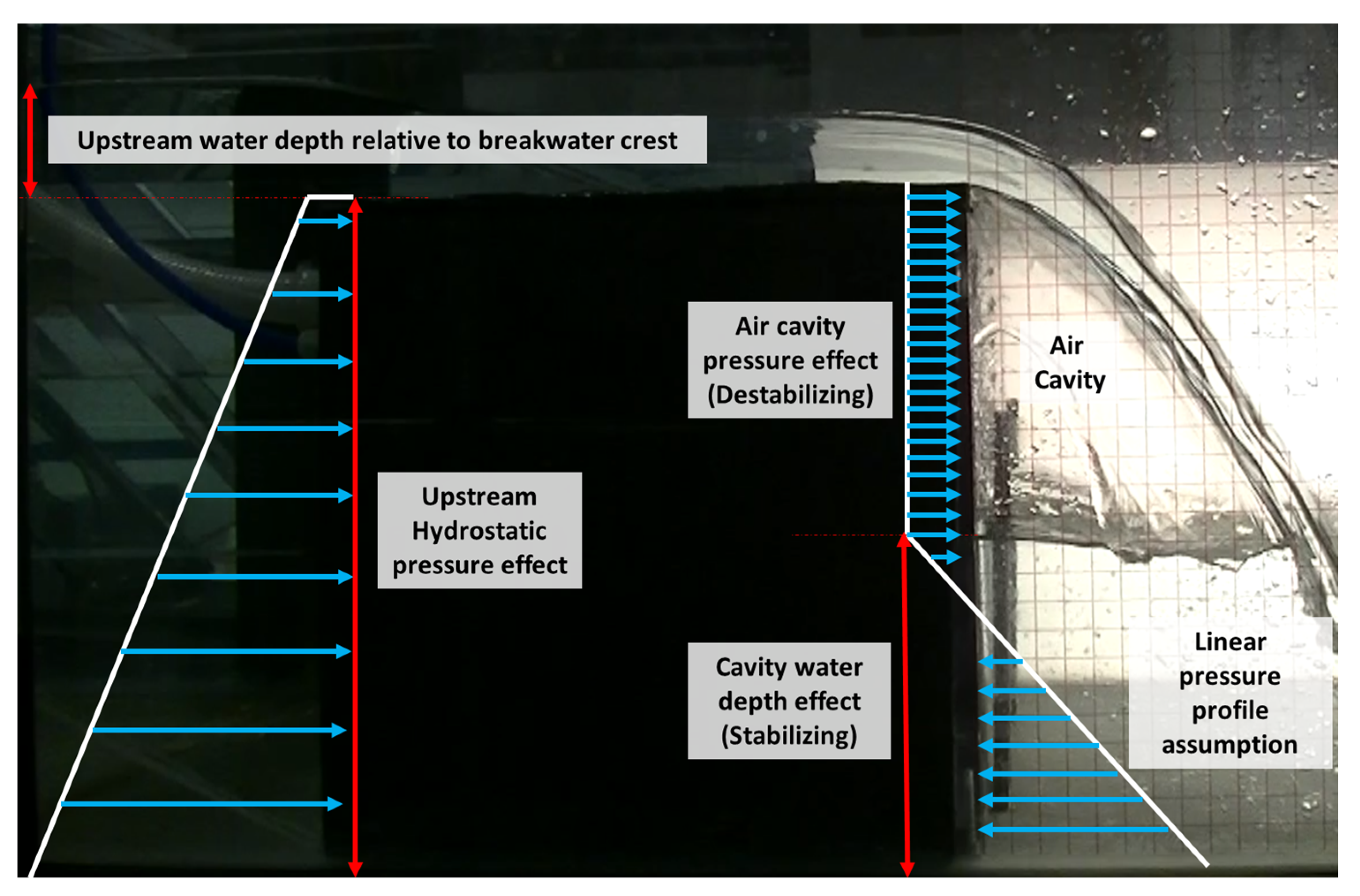
It has been widely believed that coastal long-period waves, including tsunamis, are closely related to abnormal water level rise and the overtopping of coastal breakwaters [9,10,11]. When water levels rise above a caisson breakwater due to these extreme events, the risk of sliding and overturning failures increases. During such overflow scenarios, Chanson [12] noted that air bubbles are entrained along the overflow jet and air cavity interface, as well as at its end due to a re-entrant jet mechanism (Figure 1). This entrainment causes a decrease in cavity pressure below atmospheric levels if the external air supply is interrupted, a condition referred to as non-ventilated overflow [13,14,15,16]. This phenomenon can occur in real-life situations, especially when the length of the vertical structure is considerable. Under these conditions, the importance of air cavity pressure and cavity water depth in the stability of breakwaters cannot be overstated. Sub-atmospheric pressure may develop on the leeward side of the caisson, leading to increased sliding forces and failure probability. Similarly, cavity water depth affects the sliding forces exerted on the structure. An increase in cavity water depth can stabilize the structure by providing counteracting pressure, while a decrease can lead to destabilization. Accurate prediction of these factors ensures that the design and construction of breakwaters can effectively withstand extreme conditions (Figure 2).
Despite its importance, the effect of overflow is often overlooked in the current design of vertical structures in coastal engineering. Conventional design methods, such as the Goda formula [17] for calculating wave forces, have specific limitations. One significant limitation is that the formula does not account for the effects of sub-atmospheric air cavity pressure in non-ventilated overflow scenarios. This formula, later refined by Tanimoto and Takahashi [18] to incorporate additional factors, assumes a trapezoidal pressure distribution that is only applicable when there is no overflow or when the cavity is fully ventilated during overflow. This trend persists in recent research. Yoshidal et al. [19] estimated the lift and drag forces exerted by concrete blocks for the protection of mound breakwaters through experimentation and CFD simulation. Similarly, Hess et al. [20] presented directional flow forces on vertical structures subjected to impulse waves, dividing them into cases of wave run-up and overtopping. However, neither study considered the sub-atmospheric air cavity pressure resulting from non-ventilated overflow scenarios. In the most recent version of the ASCE/SEI 7-22 Chapter 6 guideline for quasi-steady tsunami overflow of vertical structures, a constant percentage increase in force is suggested to account for the sub-atmospheric cavity pressure effect [21]. However, the actual relationship among sub-atmospheric cavity pressure, fluid properties, and structure geometry remains unknown. Surging-type tsunamis (as opposed to bore-type tsunamis) can take the form of a slowly varying flow [22]. In this situation, forces causing failure of coastal structures can be analyzed as quasi-steady limit state functions [23,24]. While wave quantities such as reflection, transmission, and dissipation coefficients are important in bore-type tsunamis, which have the characteristics of sudden shock waves, they were considered negligible in this study due to the nature of surging-type tsunamis. The gradual and steady rise in water levels allowed the analysis to focus on the water depth and its direct impact on structural stability, without the added complexity of dynamic wave interactions.
Extensive research has been conducted on dam spillway engineering on the effects of sub-atmospheric cavity pressure resulting from non-ventilated overflow scenarios. In the context of dam spillways and weirs, Michel [25] employed dimensional analysis to illustrate the relationship, termed “air demand of the cavity,” which correlates with air cavity flow rate, air cavity pressure, and the structure’s geometry. Laali and Michel [26] demonstrated a linear relationship between cavity pressure and ventilated cavity flow, along with its correlation with the Froude number. Studies by Anderson and Tullis [27], along with Lodomez et al. [28,29], suggested that using parameters like unit discharge instead of dimensionless numbers like the Froude number might better account for scale effects in overflow scenarios. Mudiyanselage [13] and Patil et al. [14] found that sub-atmospheric pressure within the cavity escalates the horizontal force acting on the weir, thus compromising structural stability during overflow. Also, experimental testing by Kim et al. [15] and computational fluid dynamic (CFD) simulations by Zou et al. [16] revealed negative cavity pressures during overflow events in the case of broad-crested weirs, but these studies did not establish a relationship between the independent (weir height, overflow depth, and downstream water depth) variables, which a designer would have available to them, and the dependent (cavity pressure) variable. Therefore, the first aim of this research is to fill this knowledge gap through laboratory experiments. Furthermore, to facilitate practical application in design and construction stages, this study aims to establish a function for air cavity pressure based on variables that can be easily obtained by other researchers.
Another unconsidered factor influencing the structural failure, besides cavity pressure, is the cavity water depth at the recirculation pool. When a nappe flow is entrained downstream, the jet experiences a sudden change in direction, and a pool of water forms immediately upstream of the nappe impact. This pool provides a horizontal pressure force, which influences the momentum balance. The ability to predict this cavity water depth is vital for estimating the pressure and force acting on the vertical structure, as an increase in cavity water depth leads to an increase in pressure and force acting in the opposite direction of water flow, while a decrease in cavity water depth results in an increase in pressure and force acting on the vertical structure.
Various researchers have aimed to predict the cavity water depth behind a falling jet, but none has presented this as functions of the parameters that a designer would have available: overflow depth, caisson height, and downstream water depth. Moore [30] suggested that insufficient ventilation could lead to the formation of a low-pressure area beneath the waterfall, as air bubbles become trapped and carried downstream. This in turn would cause the water level in the cavity to rise. Rand [31] developed empirical equations to express the dimensionless cavity water depth using the drop number as a parameter. Rajaratnam and Chamani [32] further refined the prediction by incorporating Moore and Rand’s work alongside his own data, suggesting an empirical equation for the relative depth of the pool. More recently, Toombes et al. [33] conducted experimental investigations into the cavity water depth within a recirculation pool. However, these researchers primarily focused on the supercritical flow conditions downstream of the overflowed structure. In contrast, Castillo et al. [34] proposed an empirical cavity water depth equation for subcritical downstream conditions. Nevertheless, this equation has limitations, as it requires variables such as impingement jet angle, impingement velocity, and downstream velocity, making it challenging to apply in real-world situations. The approach of the current research distinguishes itself from previous equations by proposing dimensionless equations that depend on easily measurable or predictable variables for real-world scenarios. Specifically, caisson height, upstream depth over caisson crest, and downstream water depth serve (which can be predicted via a shallow-water tsunami simulation, such as in [6,23]) as key parameters, enhancing the practical applicability of the approach.
In summary, this paper aims to predict cavity pressure and cavity water depth through hydraulic experiments, expressing these parameters as functions of easily measurable variables. This research is unique in two significant ways: (1) in the field of coastal engineering, it stands out for considering cavity pressure and cavity water depth during quasi-steady tsunami overflow, which is a knowledge gap needed for design and construction guidelines (ASCE-7); and (2) by utilizing variables that are readily measured or predicted, this approach eliminates the need for additional complex measurements, thereby enhancing its practicality.
The following sections of this paper provide a detailed exploration of the research. Section 2 describes the materials and methods used in the experiments, including the setup, independent and dependent variables, and the approach to measuring air cavity pressure and cavity water depth. Section 3 presents the results of the experiments, comparing ventilated and non-ventilated cases, and developing dimensionless equations for both air cavity pressure and cavity water depth under different downstream flow conditions. Section 4 discusses the findings, addressing the limitations of the study, the effects of downstream flow regimes, and the application of the results to prototype-scale scenarios. Section 5 concludes the research, summarizing the key insights and highlighting the significance and novelty of the study in advancing the understanding and design of hydraulic structures.

2. Materials and Methods

Experiments were conducted with a total of 30 different combinations based on three independent variables and their corresponding two dependent variables (refer to Figure 3 and Table 1). The first independent variable was the upstream water depth h u p relative to the crest, which can also be substituted as discharge using the weir equation. The second independent variable was the height of the vertical caisson breakwater h b , and the third independent variable was the downstream flume outlet height h o . The air cavity pressure p c was measured using an air pressure sensor, while the cavity water depth h c was estimated by installing a transparent grid with 0.5 inches spacing on the flume wall and recording the experiment with a video camera. The experiments were divided into two cases: the ventilated case, where external air was artificially supplied into the cavity, and the non-ventilated case, where external air was not supplied. Experiments for each case were conducted five times, with each session lasting five minutes. Assuming that the experiment reaches a steady-state condition during these trials, the analysis was performed using the mean and standard deviation of the collected data.

2.1. Flume and Vertical Caisson Breakwater Model

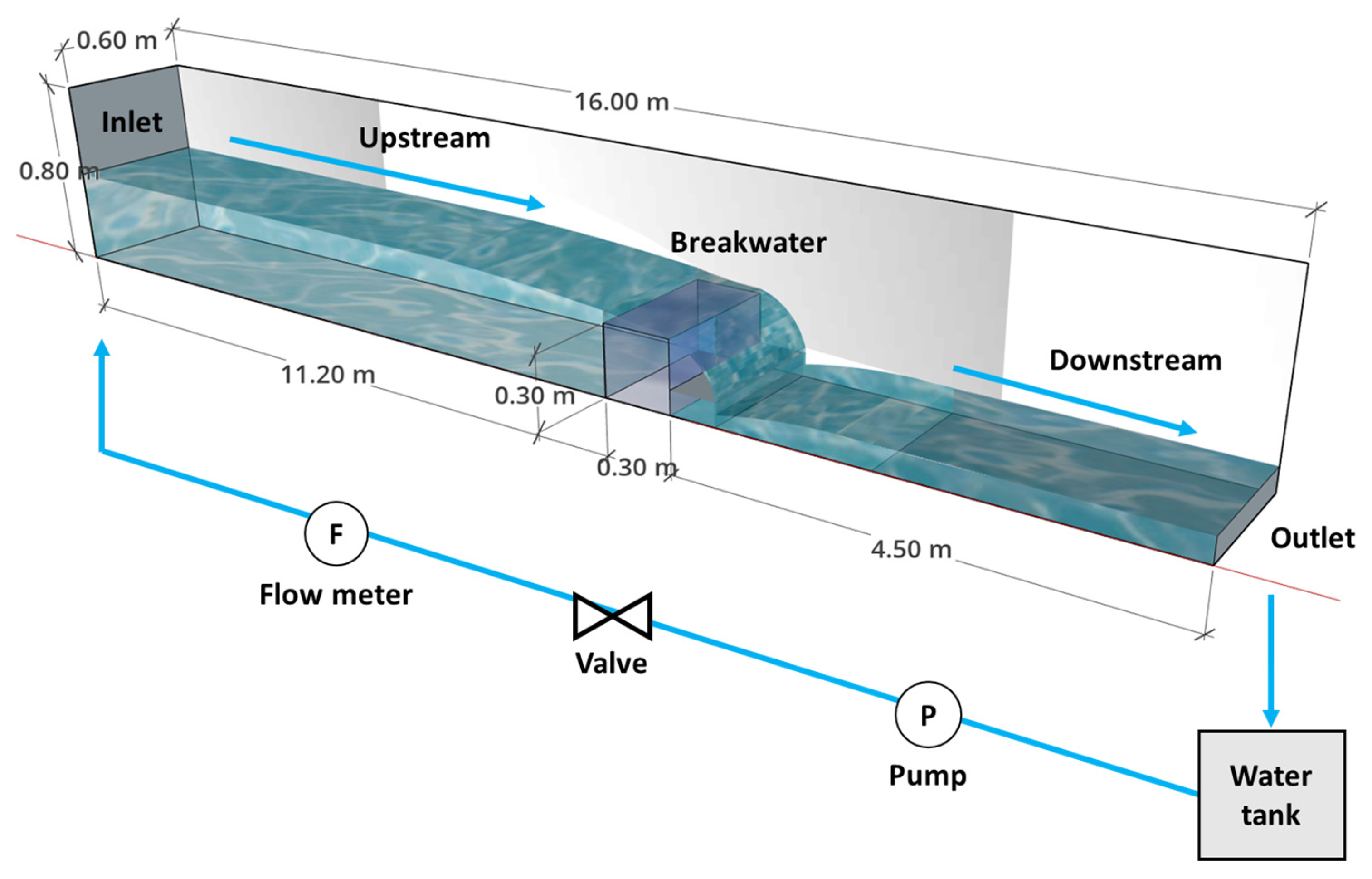
A GUNT HM 161 (G.U.N.T. Gerätebau GmbH, Barsbüttel, Germany) experimental flume, as shown in Figure 4, was utilized in the research. This flume has dimensions of 16 meters in length, 0.6 meters in width, and 0.8 meters in height. The flume’s outlet is equipped with an adjustable plate weir. For the experimental setup, a cuboid vertical caisson breakwater model, depicted in Figure 5, was specifically constructed. This model has a length of 0.3 meters in the streamwise direction ( L b ) and a cross section measuring 0.6 meters in width ( W b ) by 0.3 meters in height ( h b ). The model used for the vertical caisson breakwater in the experiments was not a scaled-down version of an actual structure. Instead, it was fabricated to precisely match the dimensions of the flume, with a width of 0.6 meters. However, with the application of a geometric and Froude scale factor, it can also be used to simulate processes at larger prototype scales such as other large caisson structures, dam spillways, and floodwalls (see the Discussion section of this manuscript).
Since this research focused on two-dimensional flow, foam pieces were wedged in the gap between the flume side wall and the model to prevent any water flow under or around the model. In the ventilated case, a snorkel made of PVC tubing was connected from the air cavity, through the model, and up to the surface, allowing for the supply of external air into the cavity. In contrast, the non-ventilated case was created by closing this tubing, halting the supply of external air. Throughout the experiments, an air pressure sensor was utilized to measure the pressure within the cavity, providing the air cavity pressure data for our analysis. A transparent grid, positioned to observe the sidewall, was employed to measure the cavity water depth. Images of the sidewall were captured by a camera at 30-second intervals over a 5-minute duration, resulting in a total of 10 readings. The average value of these measurements was used to ensure precision and reliability.

2.2. Measurement Approaches for Air Cavity Pressure and Cavity Water Depth

A Dwyer series 616KD differential pressure transmitter was employed to measure air pressure within the air cavity. This sensor, which is not waterproof, was integrated into the setup through a small tube that passed through a large snorkel. This arrangement facilitated the measurement of air cavity pressure at the snorkel’s end, positioned 2.5 cm from the crest, as illustrated in Figure 5. The air pressure recorded at this specific point was considered representative of the average pressure in the entire air cavity, given air’s much lower density compared to water. The sensor’s pressure range is limited to 3 inches of water column, equivalent to 746.52 Pa, with an accuracy of ±2% of the full-scale range, which translates to a maximum error margin of ±15 Pa. The air pressure measurements were conducted at a frequency of 83 Hz. For further details on the instruments used and their calibration, refer to Kim et al. [15].
To measure the cavity water depth in the recirculation pool, the Canny edge detection technique was utilized for a non-intrusive approach to determine fluctuating cavity water depths [35]. Given that the method prioritizes brightness over color, image pre-processing was carried out on grayscale conversions to streamline the edge detection calculations. Calibration of the system was executed using actual distances within the images.

2.3. Ventilated vs. Non-Ventilated: Air Cavity Pressure and Cavity Water Depth

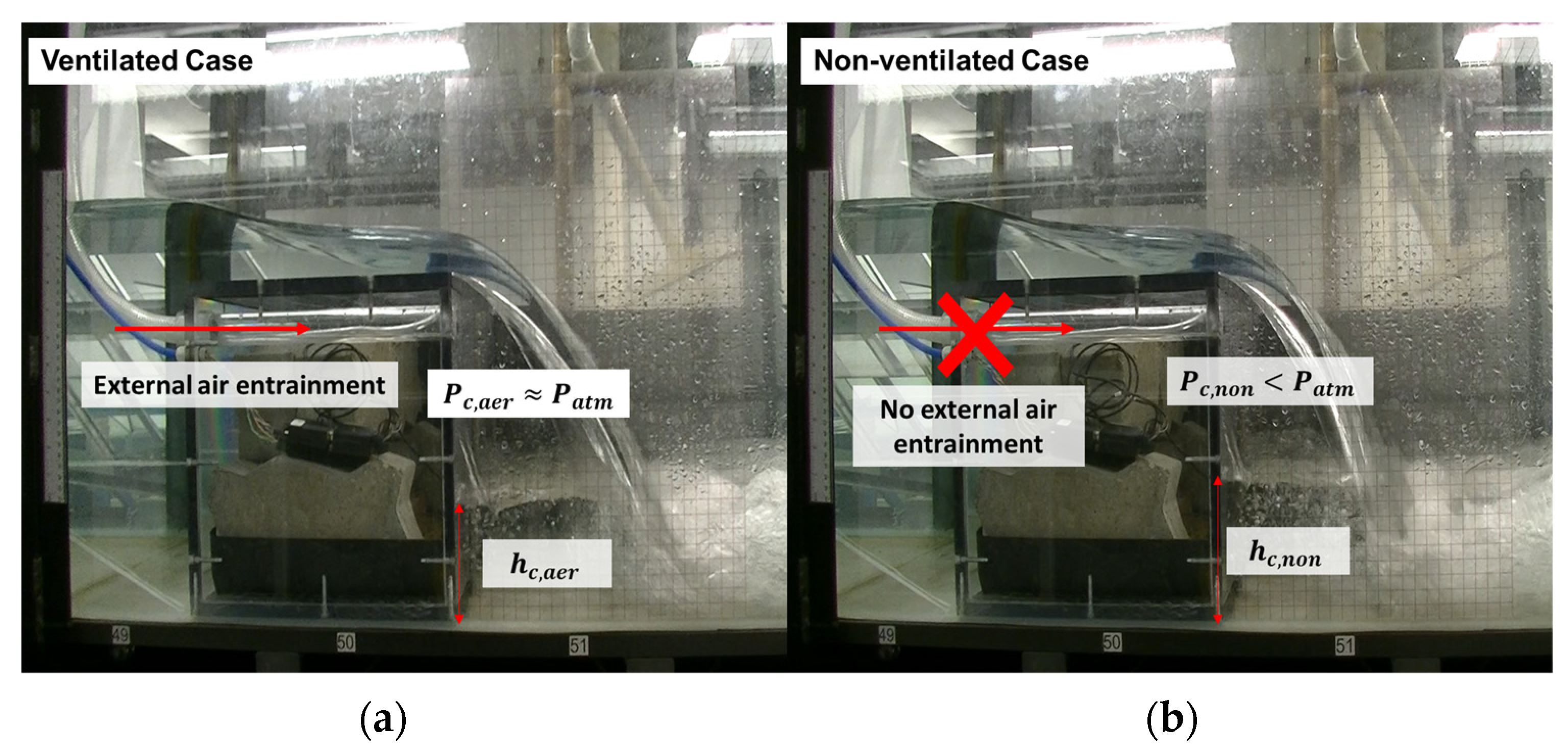
When there is external pressure in the air cavity, such as when the cavity is exposed to the atmosphere or supplied with air artificially (as in the ventilated case in Figure 6), the pressure inside the cavity p c , a e r will be close to atmospheric pressure p a t m . This is because the air inside the cavity is in equilibrium with the surrounding atmospheric pressure. However, in scenarios where there is no external air supply or air is not being replenished (as in the non-ventilated case in Figure 6), the air inside the cavity can become entrained along the nappe flow interface and at the cavity’s end. As a result, air bubbles are drawn from the air cavity into the overflowing water. The process of air entrainment and loss of external air supply can lead to a decrease in air pressure inside the cavity p c , n o n , causing it to be lower than atmospheric pressure. This decrease in pressure below atmospheric conditions is known as “sub-atmospheric pressure.”
In addition to the air cavity pressure differences, the cavity water depth in the recirculation zone plays a significant role in distinguishing between the ventilated and non-ventilated cases. In the ventilated case, the continuous supply of external air to the cavity results in a smoother and more stable water flow pattern. This minimizes disturbances and reduces the formation of a pronounced recirculation zone below the cavity. Consequently, the cavity water depth h c , a e r in the recirculation zone remains relatively lower compared to the non-ventilated case. Conversely, in the non-ventilated case, the entrainment of air from the cavity along the nappe flow interface leads to a decrease in air pressure within the cavity. This results in intermittent flow patterns and disturbances, enhancing the formation of a more pronounced recirculation zone below the cavity. As the non-ventilated cavity has lower air pressure than the ventilated case, the cavity water depth h t , n o n within the recirculation zone is elevated.

2.4. Estimating Air Flow Rate into the Cavity: A Bernoulli Equation Approach

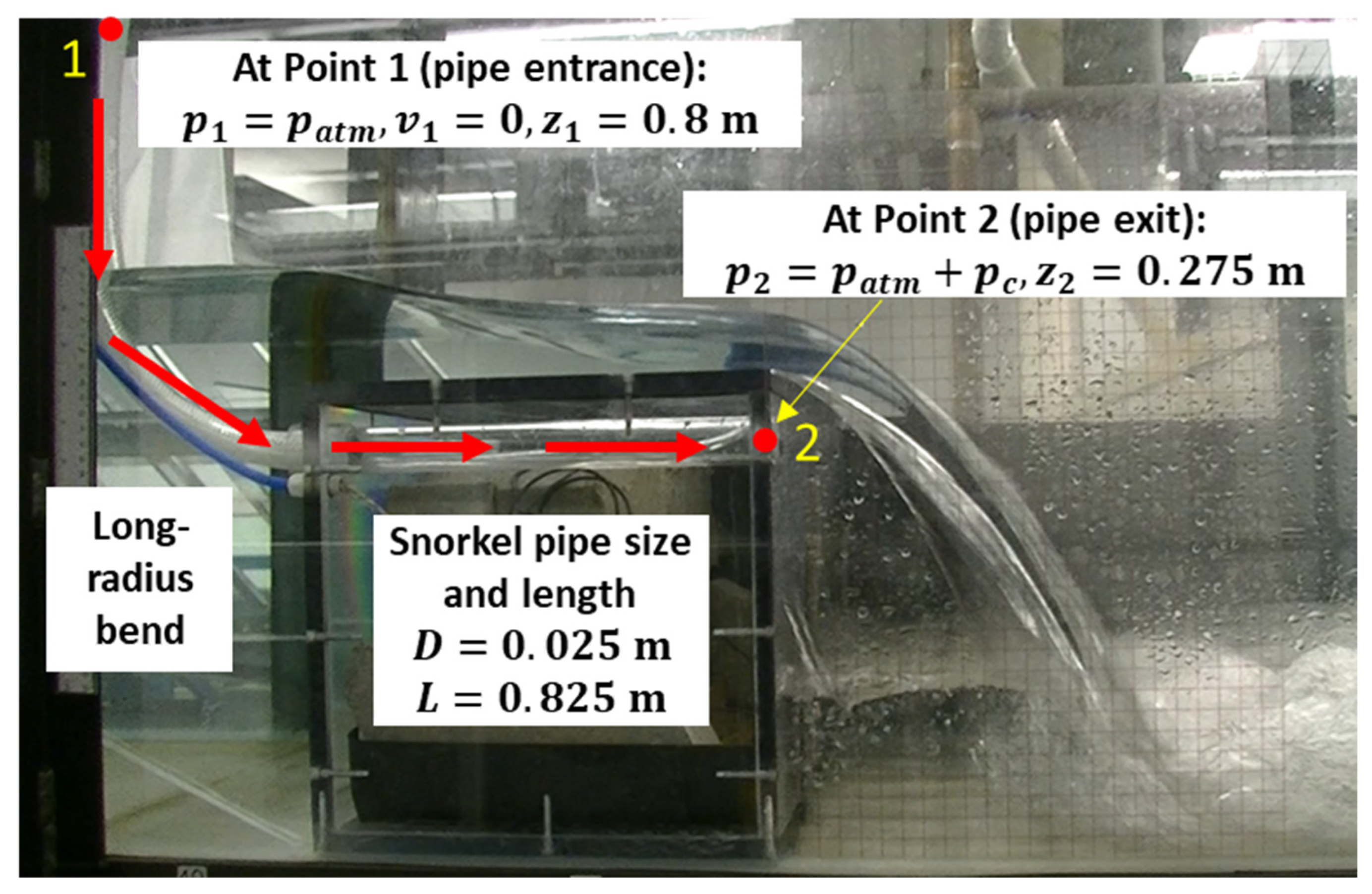
In the ventilated scenario, where the cavity is connected to the atmosphere through the snorkel, measuring air flow rate using the laboratory’s rotameter was not feasible. This was due to the minimal pressure difference between the atmosphere and the cavity, which was insufficient for rotameter operation. However, it is possible to estimate the air flow rate entering the cavity by employing the Bernoulli equation. As shown in Figure 7, Points 1 and 2 denote the endpoints of the snorkel pipe (Point 1: entrance, Point 2: exit). The Bernoulli equation can be applied as shown in Equation (1), accounting for major head losses from friction and minor losses at the snorkel entrance, a 90-degree-long radius bend, and the exit:
p 1 γ + v 1 2 2 g + z 1 h L , f r i c t i o n h L , m i n o r = p 2 γ + v 2 2 2 g + z 2
The friction head loss, h L , f r i c t i o n , is determined using the Darcy-Weisbach equation [36,37], and minor losses, h L , m i n o r , are computed based on the coefficients from Roberson et al. [38]. At Point 1 (pipe entrance), the pressure equals atmospheric pressure ( p 1 = p a t m ) with a velocity assumed to be zero ( v 1 = 0 ), and z 1 is set at 0.8 m. At Point 2 (pipe exit), the pressure is the sum of atmospheric and air cavity pressures ( p 2 = p a t m + p c ), with z 2 at 0.275 m. Incorporating these values, Equation (1) is modified to Equation (2):
p 1 γ + v 1 2 2 g + z 1 f L D v 2 2 2 g K e n + K e x + K e l v 2 2 2 g = p 2 γ + v 2 2 2 g + z 2
Here, K e n , K e x , and K e l are the minor loss coefficients for the pipe entrance, exit, and elbow, valued at 0.5, 1.0, and 0.35, respectively. L and D represent the snorkel’s length and diameter, 0.825 m and 0.025 m, respectively, and f is obtained from the Moody diagram. The final air flow rate into the cavity is calculated by multiplying the area of the snorkel pipe by the velocity v 2 derived from Equation (2).

2.5. Effects of Downstream Flow Regime on Air Cavity Pressure and Cavity Water Depth

In the experiment, a subcritical flow regime was maintained upstream, while downstream flow varied based on the independent variables: upstream water depth over the crest and downstream flume outlet height. Decreasing upstream water depth over the crest or increasing downstream flume outlet height led to subcritical flow downstream, while the opposite changes caused a shift to supercritical flow (Figure 8). To determine the downstream flow regime, the downstream water depth h d was measured at 10 points at 30-second intervals over a 5-minute period using a camera and a transparent grid similar to the cavity water depth measurement. The average values derived from these measurements were used to calculate the downstream Froude number F r d using Equation (3). A downstream Froude number less than 1 is indicative of a subcritical flow, while a value greater than 1 signifies a supercritical flow downstream. Here Q w is the water flow rate, measured using a flow meter, and g is the acceleration due to gravity.
F r d = v d g h d = Q w A d g h d = Q w 0.6 h d g h d
The different downstream flow regimes can significantly affect air cavity pressure and cavity water depth. In supercritical flow, even with increased downstream flume outlet height, the downstream water depth remained below critical depth, reducing the influence of this variable. To validate this, experiments were conducted to confirm the diminished significance of downstream flume outlet height as an independent variable in supercritical flow compared to subcritical flow. Additionally, a dimensionless equation was fitted to relate downstream flow regime, downstream flume outlet height, and other variables to gain insights into conditions affecting the system’s behavior during nappe overflow.

2.6. Dimensionless Analysis for Air Cavity Pressure and Cavity Water Depth

In this research, Buckingham’s pi theory is applied to derive dimensionless equations for both air cavity pressure and cavity water depth. As highlighted in the Introduction, air cavity pressure and cavity water depth play a pivotal role in assessing structural stability by affecting horizontal force acting on the structure. To identify the relevant variables influencing air cavity pressure, insights from Chanson [9] are referenced, which propose dimensionless analysis of air cavity pressure by considering water density, gravitational acceleration, and upstream water depth over the crest. Additionally, to enhance the practical applicability of the research findings, breakwater height and downstream flume outlet height, which are easily obtainable in real-world scenarios, are included. The downstream water depth is also included, as the Froude number downstream ( F r d ) characterizes the flow regime. Consequently, seven variables are selected: air cavity pressure ( p c ), upstream water depth over the crest ( h u p ), breakwater height ( h b ), downstream flume outlet height ( h o ), downstream water depth ( h d ), water density ( ρ ), and gravitational acceleration ( g ). Through the application of Buckingham’s pi theory, four dimensionless parameters are derived, as presented in Table 2 and expressed in Equations (4) and (5). For cases involving supercritical flow, the effect of the downstream flume outlet height can be negligible; therefore, the third dimensionless parameter is omitted, resulting in Equation (5).
Π 1 = f ( Π 2 , Π 3 , Π 4 )
Π 1 = f ( Π 2 , Π 3 )
Regarding the cavity water depth analysis, Toombes et al.’s research [33] is used as a reference, and the first dimensionless parameter, involving cavity water depth h t and vertical caisson breakwater height h b , is selected, as seen in Table 2. Additionally, for the second and fourth dimensionless parameters, the use of length ratios is adopted, following a similar approach as with the air cavity pressure. The downstream Froude number is also included as a third dimensionless parameter. As before, in the case of supercritical flow, the third dimensionless parameter is excluded, resulting in Equation (5). Based on the dimensionless equation derived from Table 2, precise relationships among the dimensionless parameters are obtained through data obtained from experiments and regression analysis (see Results section). Froude number, Weber number, and Reynolds number at the brink of the caisson breakwater were not considered as dimensionless parameters in this analysis, though they are applied to determine the validity of the results across model to prototype scales. This omission is attributed to the fact that these numbers are functions of the independent variables already considered in this study, as explained in detail in the Discussion section.

3. Results

The values of air cavity pressure and cavity water depth obtained from the experiments are examined, distinguishing between the ventilated case and non-ventilated cases. Final dimensionless equations for air cavity pressure are presented separately for the subcritical and supercritical downstream conditions. Similarly, the final dimensionless equation for cavity water depth is also presented separately for the subcritical and supercritical downstream conditions. The accuracy of each instrument was outlined in Section 2. To evaluate the level of accuracy, uncertainty in the final results is quantified via error bars and confidence intervals in the figures. Error bars represent the standard deviations of the measured values, indicating variability within the trials. The shaded areas show the 95% confidence intervals for the ventilated and non-ventilated conditions, derived from the regression equations. Performance metrics, including the correlation coefficient (R), the coefficient of determination (R²), and the root mean squared error (RMSE), are used to assess the model fit. High R and R² values and low RMSE values indicate strong correlations and minimal deviations between the predicted and actual values, confirming the accuracy of the model. Additionally, the representative mean and standard deviation are calculated using variances from each trial, ensuring accurate capture of variability across trials to ensure the reliability of the data

3.1. Comparison of Ventilated and Non-Ventilated Cases for Air Cavity Pressure and Cavity Water Depth

Table 3 presents the representative average values for air cavity pressure ( p c ), cavity water depth ( h c ), and downstream water depth ( h d ) across different variables. To ensure reliability, each of the 30 experimental cases was repeated five times. For statistical analysis, we calculate the representative mean ( x ¯ ) of the data, which is the average of the means ( x ¯ 1 , x ¯ 2 , x ¯ 3 , x ¯ 4 , x ¯ 5 ) from the five trials. The representative standard deviation ( s p ), which accounts for variability across all trials, is calculated using the variances from each trial and their respective degrees of freedom (total number of observations in each trial minus one). The representative average values and standard deviations for air cavity pressure and cavity water depth, along with the average values and standard deviations for each trial, are detailed in Appendix A and Appendix B, respectively.
As depicted in Table 3, the air cavity pressure in the non-ventilated case is lower than in the ventilated case, which aligns with Chanson’s study [12]. For the non-ventilated case, the air cavity pressure exhibits a negative correlation with increasing upstream water depth over the crest. Conversely, in the ventilated case, the air cavity pressure is close to zero (gauge pressure) for low upstream water depths over the crest ( h u p = 0.055 , 0.061 , 0.065 m ), but negatively increases for high upstream water depths over the crest ( h u p = 0.083 , 0.101 m ). This suggests that the cavity undergoes a transition from a fully ventilated condition to a partially ventilated condition as the upstream water depth over the crest increases and implies that the flow rate of external air entering the cavity may also influence the air cavity pressure. This hypothesis is tested using the Bernoulli equation approach, and the results are shown in Table 3. Air flow rate calculations are conducted only for the ventilated case, as the non-ventilated case blocks external air inflow, resulting in zero air flow rate into the cavity. The absolute roughness of the pipe, ε, is set at 0.046 mm for the calculations, as a new smooth plastic pipe is used. The friction factor, f , obtained from the Moody diagram, is 0.040, with the Reynolds number ranging between 2464 and 5716, as seen in Table 3. Using this friction factor in Equation (2), the air flow rate results in Table 3 show that the lowest air flow rate corresponds to a fully ventilated case with cavity pressure close to zero. As the condition becomes partially ventilated and cavity pressure increases negatively, there is a tendency for the supplied air flow rate to increase.
It is observed that the non-ventilated case exhibits deeper cavity water compared to the ventilated case. This finding is consistent with the results of studies conducted by Toombes et al. [33] and Mudiyanselage [13], indicating that non-ventilated overflow creates lower pressure in the air cavity, pulling upward on the cavity water and leading to an increase in cavity water depth. This increased cavity water depth results in higher downstream water pressure acting on the breakwater, which can be verified through measurements from water pressure sensors. The downstream flow regime was determined by comparing the downstream water depth observed in videos with the critical depth. Among the 15 cases listed in Table 3, 11 cases exhibited a subcritical downstream flow regime, while 4 cases showed a supercritical downstream flow regime. It was observed that increasing upstream water depth over the crest and decreasing downstream flume outlet height tended to shift the flow regime from subcritical to supercritical, in accordance with the tendencies predicted by the Froude number equation.

3.2. Dimensionless Equation for Air Cavity Pressure with Subcritical Flow Downstream

Figure 9 gives a graphical representation of the dimensionless equation developed for air cavity pressure in a subcritical downstream scenario. To determine the most suitable form of the dimensionless equation, regression analysis was conducted using both linear and quadratic regression. The values on the x-axis represent either a linear or quadratic regression model for parameter 1 ( Π 1 = p c ρ g h u p ), which is related to various other dimensionless parameters. Meanwhile, the y-axis represents the corresponding experimental values of parameter 1.
In the graphs, average values for the ventilated condition are marked with blue circles, while those for the non-ventilated condition are indicated by black circles. Vertical error bars extending from each circle represent the standard deviation. The shaded areas in blue and black show the 95% confidence intervals (CIs) for the ventilated and non-ventilated conditions, respectively, based on their regression equations. The width of the confidence intervals along the x-axis varies depend on the standard deviations obtained from each trial for each case. A larger standard deviation in a specific case results in a wider confidence interval, and vice versa. For cavity pressure, the non-ventilated condition generally exhibits wider confidence intervals than the ventilated condition. This difference is primarily due to the non-ventilated condition experiencing fluctuations in gauge pressure as a result of being sealed off from external air, leading to negative pressures within the cavity. In contrast, the ventilated condition maintains a pressure close to atmospheric due to the continuous external air supply, resulting in nearly zero-gauge pressure. These fluctuations in the non-ventilated condition are further influenced by air being entrained into the cavity through nappe flow.
To determine the best regression model between the linear and quadratic options, three key indicators were utilized: (1) the correlation coefficient ( R ), (2) the coefficient of determination ( R 2 ), and (3) the root mean squared error (RMSE). The model with higher R and R 2 values and lower RMSE was selected as the more accurate. When differences between the models were minimal, linear regression was preferred for its efficiency. In the scenario of quadratic regression, the alignment of data points with the fitted curve was noticeably better than with linear regression, as evidenced by higher R and R 2 values and a lower RMSE, as illustrated in Figure 9. This indicates that the quadratic model provides a more accurate prediction of air cavity pressure in this subcritical downstream scenario compared to the linear model.
Table 4 displays the final quadratic dimensionless equation for air cavity pressure in the subcritical downstream scenario between the ventilated and non-ventilated conditions, along with its performance. The equation obtained is in the following form, with each coefficient value listed in Table 4. Various performance factors were used to assess the goodness of fit of the model. For the ventilated scenario, the model demonstrates a correlation coefficient ( R ) of 0.984 and a coefficient of determination ( R 2 ) of 0.969, coupled with a root mean squared error (RMSE) of 0.001. These values indicate a strong correlation and minimal deviation between the predicted and actual observations. In contrast, the non-ventilated scenario exhibits even stronger performance metrics, with an R value of 0.995, an R 2 of 0.989, and an RMSE of 0.003. This indicates a slightly greater variability, but still provides outstanding predictive accuracy.

3.3. Dimensionless Equation for Air Cavity Pressure with Supercritical Flow Downstream

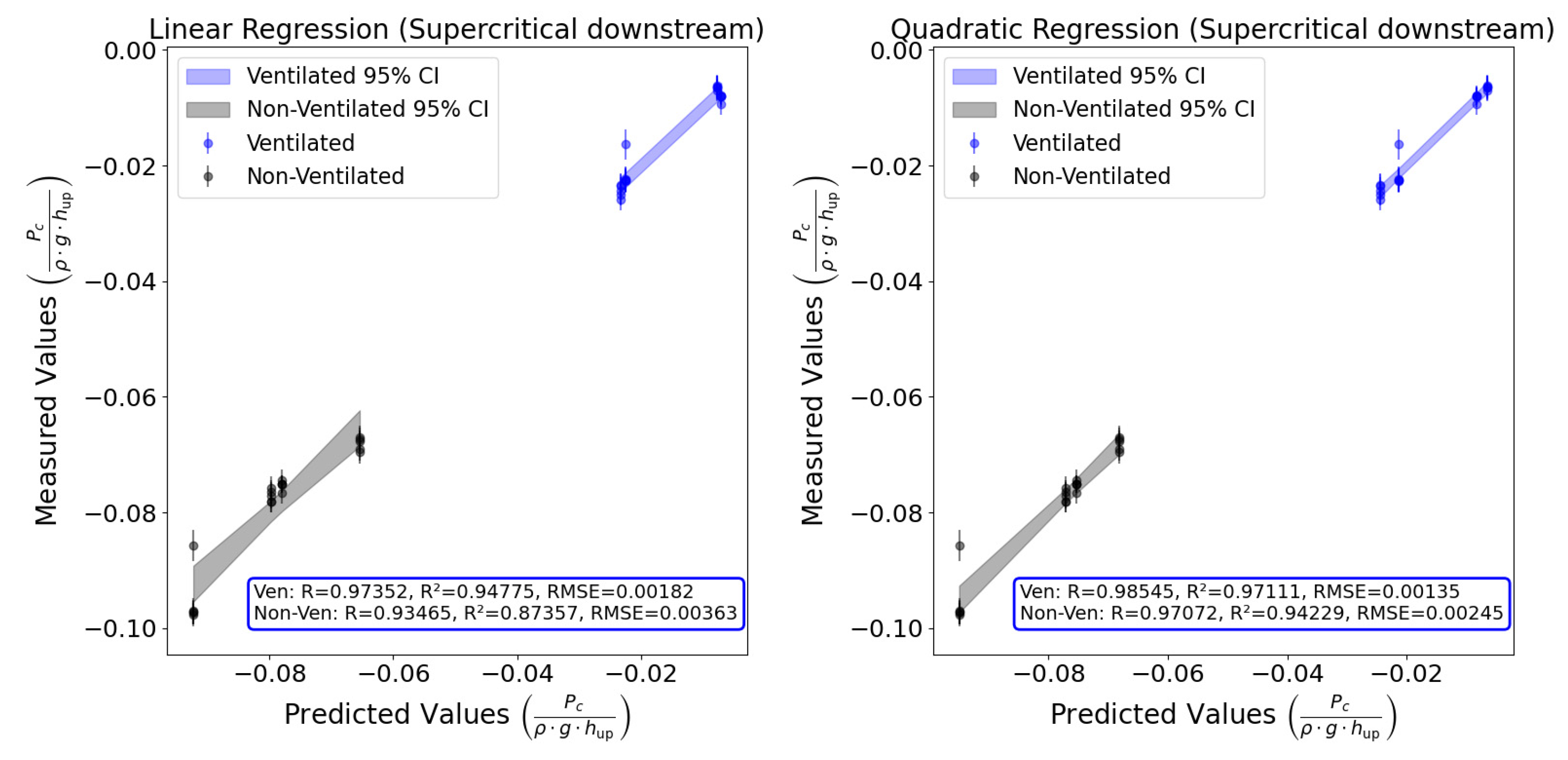
The methodology applied in the subcritical downstream case was also utilized in the supercritical downstream scenario to derive a dimensionless equation for air cavity pressure. Figure 10 illustrates this dimensionless equation, visually representing its development. As observed in the subcritical case, the performance of quadratic regression surpasses that of linear regression in the supercritical scenario, as indicated by the performance indicators displayed in Figure 10. Consequently, the final dimensionless equation for the supercritical downstream scenario includes second-order terms for all dimensionless parameters, mirroring the approach taken in the subcritical case.
Table 5 presents the final dimensionless equation for air cavity pressure in the supercritical downstream scenario, along with the assessment of its goodness of fit. This evaluation utilized several performance metrics. For the ventilated condition, the model demonstrates an R of 0.985 and an R 2 of 0.971, with an RMSE of 0.001. These metrics indicate a high degree of correlation and minimal average deviation between the predicted and actual values, showcasing strong predictive accuracy. Conversely, the non-ventilated condition shows strong performance metrics as well, with an R of 0.971, an R 2 of 0.942, and an RMSE of 0.002. This suggests slightly higher variability compared to the ventilated condition, but still provides excellent overall predictive accuracy.
In the analysis of the supercritical downstream case, it is notable that the coefficients associated with the dimensionless parameters Π 2 and Π 3 ( β 1 , β 2 , β 4 , β 5 , β 7 ) are predominantly close to zero, in contrast to the subcritical downstream case, where these coefficients were non-zero. This indicates a reduced significance of Π 2 or Π 3 in predicting air cavity pressure in the supercritical downstream scenario, underscoring the necessity to tailor dimensionless equations to specific flow conditions, which helps simplify the model and minimize the risk of overfitting.
To further investigate the dynamics in the supercritical downstream scenario, additional dimensionless analyses were performed by separately excluding parameter 2 ( Π 2 ) or parameter 3 ( Π 3 ), prompted by their negligible coefficients in the supercritical downstream case. These analyses resulted in a simplified dimensionless equation involving only three parameters. A comparison of the dimensionless equations and goodness-of-fit metrics between Table 5 and Table 6 shows a striking similarity, confirming that ( Π 2 ) has minimal impact on estimating air cavity pressure in supercritical downstream conditions. Similarly, excluding ( Π 3 ), which represents the downstream Froude number, it does not significantly alter the estimation of air cavity pressure either, suggesting it is not a critical factor in this scenario. However, the removal of parameter 3 ( Π 3 ) results in significantly larger coefficients in the dimensionless equation, indicating a potential instability in the model when this parameter is excluded.
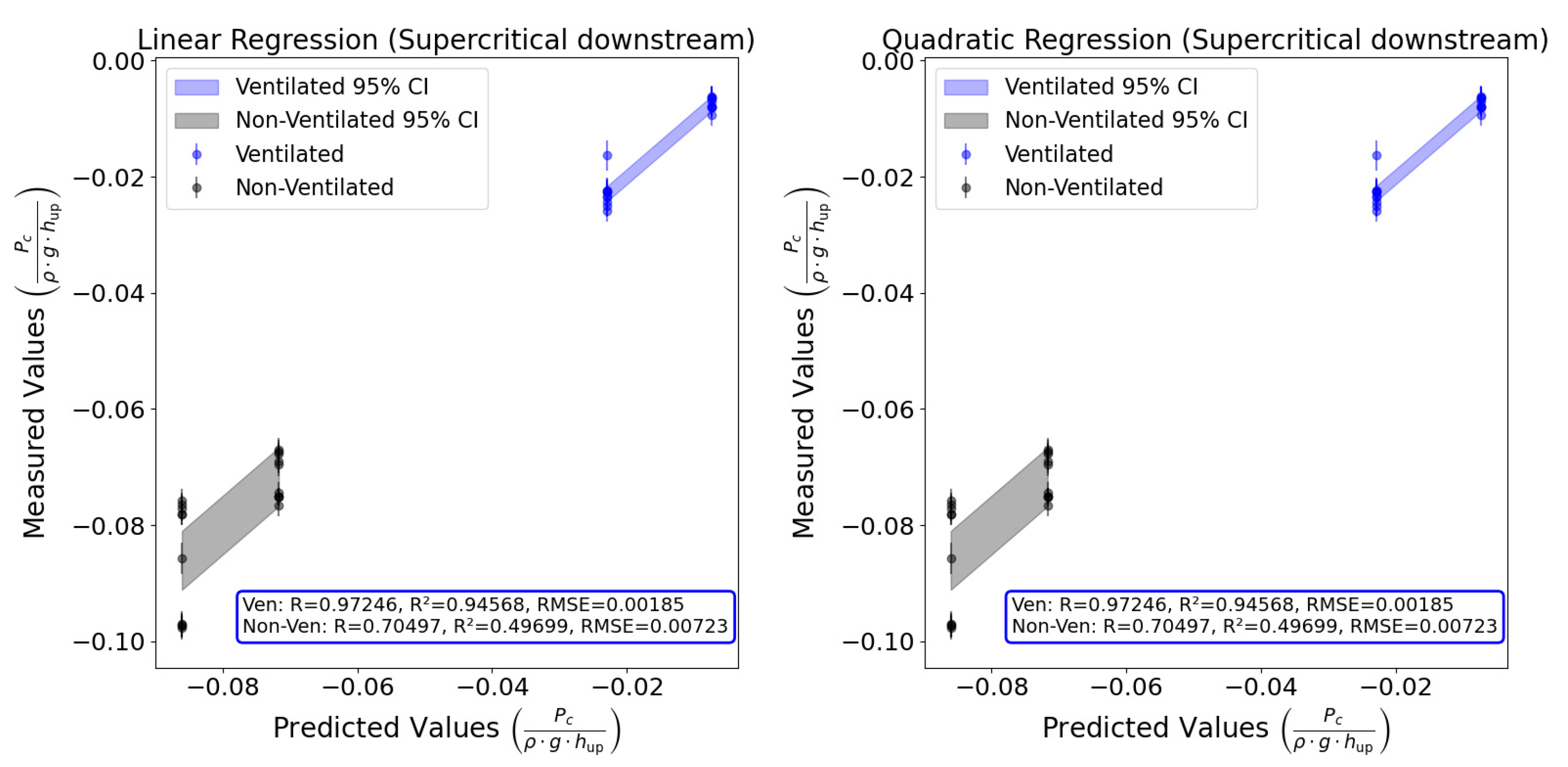
The second dimensionless analysis involves excluding parameter 4 ( Π 4 ), based on the hypothesis that the downstream flume outlet height should have negligible effects upstream in supercritical flow. However, Figure 11, which excludes ( Π 4 ), shows notably lower goodness-of-fit metrics compared to Figure 10, where all four dimensionless parameters were considered. This is particularly evident in the non-ventilated conditions. The R-squared value of 0.705 for both linear and quadratic regression indicates a relatively strong correlation, but is significantly lower than the 0.971 achieved when including all parameters. This discrepancy can be attributed to issues with the accuracy of the air pressure sensor and the limited number of experimental cases for supercritical downstream conditions compared to subcritical conditions. By increasing the number of supercritical experiments and using a more accurate sensor, a stronger correlation between the variables is expected to emerge.

3.4. Dimensionless Equation for Cavity Water Depth with Subcritical Flow Downstream

In the subcritical downstream scenario, a regression analysis was performed to establish the final dimensionless equation for cavity water depth using a different set of dimensionless parameters compared to those used for air cavity pressure. The first dimensionless parameter was adapted to reflect cavity water depth ( Π 1 = h c h b ), while the second, third, and fourth parameters ( Π 2 , Π 3 , Π 4 ) remained consistent.
Figure 12 graphically represents the dimensionless equation developed for cavity water depth. One notable feature observed in Figure 12 is that the cavity water depth measured under non-ventilated conditions is greater than that measured under ventilated conditions. This observation supports the theoretical explanation provided in the Materials and Methods section, which posits that cavity water depth is greater in non-ventilated conditions than in ventilated conditions. Regarding the dimensionless equation for cavity water depth in the subcritical downstream scenario, unlike with air cavity pressure, the performance metrics for both linear and quadratic regressions showed nearly identical results. Consequently, the simpler linear regression model was selected as the final dimensionless equation. Table 7 outlines the goodness-of-fit metrics and performance values for this equation, highlighting an impressive R-squared value of 0.969 for ventilated and 0.989 for non-ventilated conditions, indicating strong correlations. The final chosen equation incorporates first-order terms for all involved dimensionless parameters, as detailed in Table 7. This model effectively captures the dynamics of cavity water depth in the subcritical downstream scenario, as evidenced by high R values of 0.984 for ventilated and 0.995 for non-ventilated conditions, and minimal RMSE values of 0.001 and 0.003, respectively.

3.5. Dimensionless Equation for Cavity Water Depth with Supercritical Flow Downstream

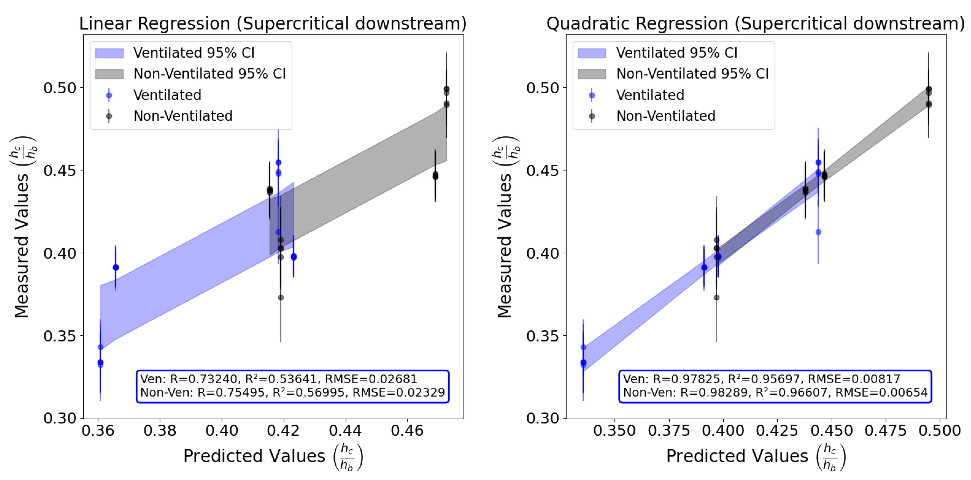
In the supercritical downstream scenario, Figure 13 depicts the comparison of linear and quadratic regression models for cavity water depth. The quadratic regression outperforms the linear model, demonstrating significantly stronger performance metrics. Specifically, quadratic regression achieves R values above 0.97 and R 2 values close to or above 0.96, along with lower RMSE values (0.008 for ventilated and 0.007 for non-ventilated conditions), indicating a superior fit and enhanced predictive accuracy. In contrast, the linear regression yields lower R 2 values (0.536 for ventilated and 0.610 for non-ventilated) and higher RMSEs (0.027 and 0.023), suggesting it is less effective at capturing the dynamics of cavity water depth under supercritical conditions.
In the analysis of cavity water depth for the supercritical downstream case, as detailed in Table 8, it is observed that the coefficients for the dimensionless parameters Π 2 and Π 3 ( β 1 , β 2 , β 4 , β 5 , β 7 ) are predominantly close to zero. This finding mirrors the results seen in the air cavity pressure case, suggesting that Π 2 and Π 3 have limited influence on predicting cavity water depth under these conditions.
Similar to the approach taken with air cavity pressure, additional dimensionless analyses were carried out by omitting parameter 2 ( Π 2 ) or parameter 3 ( Π 3 ) independently. When comparing the dimensionless equations and the corresponding goodness-of-fit metrics between Table 8 and Table 9, the results show remarkable consistency, demonstrating that Π 2 has little effect on predicting cavity water depth in supercritical downstream conditions. Likewise, the exclusion of Π 3 , which denotes the downstream Froude number, appears to have a negligible impact on the model’s accuracy in estimating cavity water depth, indicating its limited relevance in this context. Nonetheless, eliminating Π 3 leads to considerably larger coefficients in the dimensionless equation, suggesting that the model may become less stable without this parameter.
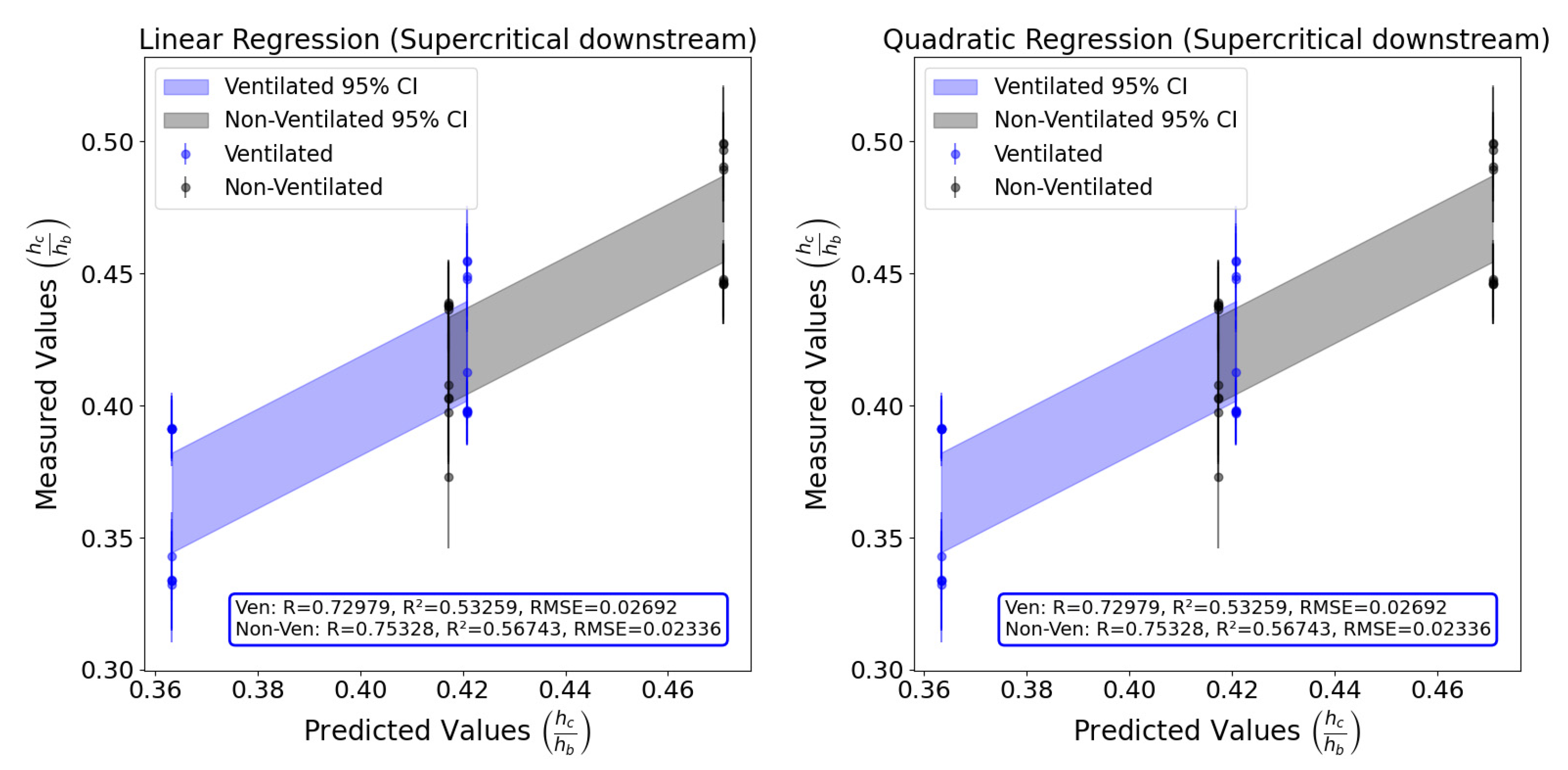
The regression analysis in Figure 14, which excludes parameter 4 ( Π 4 ), related to the downstream flume outlet height in the supercritical downstream scenario, reveals significant insights. This exclusion was based on the hypothesis that the downstream flume outlet height would minimally impact upstream conditions. Despite this, the goodness-of-fit metrics in Figure 14 for both ventilated and non-ventilated conditions show significant declines compared to scenarios where all parameters are included, as shown in Figure 13. Specifically, the R 2 values for quadratic regression are much lower (0.533 for ventilated conditions and 0.567 for non-ventilated conditions), indicating a weaker correlation. In contrast, when all parameters were considered, the R 2 values were substantially higher: 0.957 for ventilated and 0.966 for non-ventilated conditions. This notable discrepancy, similar to the air cavity pressure case, underscores potential limitations of this study.

4. Discussion

Despite the promising goodness-of-fit metrics observed in the predictions of cavity water depth and air cavity pressure, this experimental study faces several limitations. These include a limited number of data points for supercritical downstream flow cases, reliance on steady-state assumptions for analyzing time-averaged values, and discrepancies arising from differences between the model and the prototype scale. Each of these limitations is explored in greater depth below.

4.1. Limited Data for Supercritical Downstream Case

The scarcity of data points for the supercritical downstream case presents a notable limitation in this study. As a result, the dimensionless equations for air cavity pressure and cavity water depth with supercritical downstream flow conditions are not as robust as the subcritical downstream flow scenario. To address this limitation, future research should prioritize the expansion of the dataset for the supercritical downstream flow case. This may entail conducting additional experiments or employing numerical simulations to generate more data points, thus enhancing the reliability and accuracy of the derived dimensionless equations for the supercritical condition.

4.2. Steady-State Assumption

The analysis in this study is based on time-averaged values and standard deviations of air cavity pressure and cavity water depth under the assumption of steady-state conditions. Alongside the mean values, error bars representing standard deviations are also presented in the results. However, notable fluctuations in nappe and cavity water behavior were observed in some non-ventilated scenarios. Future research should aim to measure instantaneous values of air cavity pressure and cavity water depth. Such studies could illuminate the dynamic relationships between independent and dependent variables, offering insights into real-time interactions within these systems.

4.3. Scale Effect

To extrapolate laboratory data to prototype-scale applications successfully, it is essential to consider scale-dependent effects by ensuring similarity between the model and the actual system. This involves achieving geometrical, kinematic, and dynamic similarity. However, to comprehensively address scale-dependent effects, it is evident that kinematic and dynamic similarity should be considered as well, as achieved through the well-known dimensionless Froude number, Weber number, and Reynolds number.
The reason these three dimensionless numbers were not included as dimensionless groups is that they are already expressed as functions of the independent variables. Including them would introduce redundancy into the analysis. Based on the work of Mäkiharju [39], the Froude number, Weber number, and Reynolds number based on the brink of the caisson breakwater are defined as Equations (6)–(8) by considering definitions and the continuity equation.
F r b r = U b r g h b r = Q u p g h b r 1.5 W b
W e b r = ρ U b r 2 h b r σ = ρ Q u p 2 σ h b r W b 2
R e b r = ρ U b r h b r μ = ρ Q u p μ W b
In Equations (6)–(8), all variables except for the upstream flow discharge ( Q u p ) and the water depth at the brink ( h b r ) are constants. These constants include gravity acceleration ( g ), crest width ( W b ), water density ( ρ ), water surface tension ( σ ), and dynamic viscosity of water ( μ ).
By incorporating the critical flow depth (Equation (9)) and the experimental formula (Equation (10)) proposed by Rouse [40], and Francis weir formula (Equation (11)):
h c r i t = Q u p 2 g W b 2 3
h b r = 0.715 h c r i t
Q u p 2 3 C 1 W b 2 g h u p 1.5
Equations (6)–(8) can be rewritten as Equations (12)–(14). Here, h c r i t is the critical depth.
F r b r = Q u p g h b r 1.5 W b = g h c 1.5 W b g h b r 1.5 W b = h c r i t h b r 1.5 h c r i t 0.715 h c r i t 1.5 = 1 0.715 1.5 1.654
W e b r = ρ Q u p 2 σ h b r W b 2 = ρ Q u p 2 σ 0.715 h c r i t W b 2 = ρ Q u p 4 3 σ 0.715 W b 4 3 = f h u p
R e b r = ρ Q u p μ W b = f h u p
As can be seen in Equations (12)–(14), at the brink of the breakwater, the Froude number, Weber number, and Reynolds number are either constant or can be expressed as functions of one of the independent variables (the upstream depth relative to crest). Consequently, there is no need for separate measurements of the Froude number, Weber number, or Reynolds number, as their values can be estimated from the independent variables, as summarized in Table 10.
Referring to the calculated values of the Froude number, Weber number, and Reynolds number from Table 10, the regression equations presented in this study are expected to perform well and be applicable under the condition of a vertical caisson breakwater, especially when the Weber number at the brink of the breakwater falls within the range of 200 to 700. Surface tension is deemed negligible, as the Weber number consistently exceeds the critical value of 120 [41]. Therefore, the findings of this research are especially pertinent in scenarios where surface tension at the brink can be ignored. Consequently, the accuracy of the regression equations remains stable for large Weber numbers, where surface tension is negligible. For this experiment, the Froude number at the brink remains constant, likely approximating the value of 1.654 in any scenario. Regarding the Reynolds number, the values shown in Table 10 indicate that in all cases, the Reynolds number at the brink exceeds 4000, indicating fully turbulent flow. This aligns well with larger-scale civil engineering applications, demonstrating that the regression equations from this study accurately reflect turbulent flow conditions where surface tension can be disregarded.
Prior studies have investigated the scale effect on air-water flow properties in stepped spillways. Notably, Felder and Chanson [42] concentrated on the nappe flow regime and discerned that specific air-water flow properties could be effectively scaled for a model at a 1:2 scale. Nevertheless, they also noted that other parameters did not scale appropriately, underlining the intricacies of scale effects. In Felder et al.’s subsequent work [43], laboratory experiments were conducted at the prototype scale on a stepped spillway chute. However, these experiments did not directly address the scale effect on our study’s dependent variables: air cavity pressure and cavity water depth. Consequently, the precise impact of scale on these parameters remains unexplored. To advance our comprehension further, future research should explicitly investigate the influence of scale on cavity water depth and cavity pressure.

5. Conclusions

This research investigates the characteristics of air cavity pressure and cavity water depth in an open-channel flow scenario, with a particular focus on the influence of flow conditions and hydraulic parameters. By examining these factors, the research aims to enhance our understanding of the behavior of hydraulic structures and their stability, as well as contribute to the design and optimization of such structures for improved performance and safety.
(1)
Key Findings
(a)
This study is the first to express air cavity pressure and cavity water depth as functions of structure height, overflow depth, and outlet height, rather than the traditionally used unit flow discharge, making it more applicable to real-world design and construction.
(b)
The comparative analysis of ventilated and non-ventilated cases reveals a significant influence of cavity ventilation on air cavity pressure and cavity water depth.
(c)
Specifically, the non-ventilated case demonstrates lower air cavity pressure compared to the ventilated case, corroborating findings from previous research.
(d)
The non-ventilated case typically features deeper cavity water, aligning with historical data.
(2)
Derived Equations
(a)
Dimensionless equations for both air cavity pressure and cavity water depth across subcritical and supercritical downstream flow conditions illuminate the relationships between various hydraulic parameters-such as structure height, overflow depth, and flume outlet height-and the dependent variables.
(b)
The analysis showcases strong correlations with high R-squared values, underscoring the precision and robustness of the equations.
(c)
For air cavity pressure, the quadratic dimensionless equation was identified as the best model across different downstream flow regimes.
(d)
For cavity water depth, the linear equation was most suitable for subcritical conditions, while the quadratic equation provided the best fit in supercritical conditions.
(3)
Practical Applications
(a)
This study helps accurately estimate the pressure acting on structures during extreme cases, such as tsunami-induced overtopping of breakwaters. By integrating the pressure profile, it is possible to estimate the forces acting on the structure, enabling safer design.
(b)
Given that the experiments were conducted with appropriate Froude, Weber, and Reynolds numbers, the developed nondimensional regressions can be effectively utilized by engineers to estimate air cavity pressure and cavity water depth at prototype scale for civil engineering applications such as dam spillways, floodwalls, and caissons.
(c)
This will allow determination of the full horizontal force on a structure, from which design to resist sliding, overturning, and foundation punching can be robustly calculated.
(d)
The findings are applicable not only in coastal engineering but also in any scenario where overtopping causes a structure to function as a weir.
(4)
Limitations and Future Work
(a)
The scarcity of data points for supercritical downstream conditions limits the robustness of the derived equations. Future research should expand the dataset through additional experiments or numerical simulations.
(b)
The study’s reliance on time-averaged values under steady-state conditions may not fully capture dynamic behaviors. Future research should measure instantaneous values to understand real-time interactions.
(c)
Extrapolating laboratory data to prototype-scale applications requires considering scale-dependent effects. Future research should investigate the influence of scale on cavity water depth and pressure to ensure applicability across different scales.

Author Contributions

Conceptualization, T.K. and J.D.B.; methodology, T.K. and J.D.B.; software, T.K., J.N.M. and S.S.; validation, T.K., J.N.M.; formal analysis, T.K., J.N.M. and S.S.; investigation, T.K., J.N.M. and S.S.; resources, J.D.B.; data curation, T.K.; writing-original draft preparation, T.K.; writing-review and editing, T.K. and J.D.B.; visualization, T.K., J.N.M. and S.S.; supervision, J.D.B.; project administration, J.D.B. All authors have read and agreed to the published version of the manuscript.

Funding

This research received no external funding.

Institutional Review Board Statement

Not applicable.

Informed Consent Statement

Not applicable.

Data Availability Statement

The data presented in this study are available on request from the corresponding author.

Acknowledgments

The authors extend their heartfelt gratitude to the laboratory technicians in the Civil and Environmental Engineering Department at the University of Michigan for their invaluable contributions. Special thanks go to Jan Pantolin for providing guidance on the use of experimental equipment. Additionally, Steve Donajkowski and Justin Roelofs offered valuable assistance in the fabrication of the vertical caisson breakwater used in the experiments. Ethan Kennedy’s support in establishing the data acquisition system is greatly appreciated. Once again, the authors express their sincere thanks to all of them for their invaluable support and assistance throughout the research process.

Conflicts of Interest

The authors declare no conflicts of interest.

Appendix A

Appendix A provides detailed supplementary data crucial for understanding the main research findings. Table A1 and Table A2 present a comparative analysis of average cavity pressures and their standard deviations for both ventilated and non-ventilated cases under various experimental conditions.
Table A1. Comparative analysis of average cavity pressures in ventilated and non-ventilated cases.
Independent VariablesAverage Cavity Pressure, p ¯ c [Pa]
Ventilated CaseNon-Ventilated Case
h u p [m] h b [m] h w [m] p ¯ c , v 1 p ¯ c , v 2 p ¯ c , v 3 p ¯ c , v 4 p ¯ c , v 5 p ¯ c , v 1 p ¯ c , n 1 p ¯ c , n 2 p ¯ c , n 3 p ¯ c , n 4 p ¯ c , n 5 p ¯ c , n 1
0.0550.3000.1000.01−0.030.000.00−0.02−0.01−29.58−29.74−29.44−27.21−28.43−28.88
0.0610.3000.100−0.04−0.01−0.05−0.05−0.04−0.04−33.48−32.87−33.91−35.82−34.05−34.02
0.0650.3000.100−0.05−0.05−0.04−0.04−0.04−0.04−37.99−38.02−38.55−37.36−38.69−38.12
0.0830.3000.100−6.53−6.44−6.52−6.47−7.57−6.70−61.10−61.15−61.15−60.61−62.36−61.27
0.1010.3000.100−22.18−22.44−22.35−22.28−16.17−21.08−96.04−96.79−96.44−96.32−84.88−94.09
0.0550.3000.1250.04−0.04−0.02−0.04−0.04−0.02−34.51−34.47−34.93−32.90−34.56−34.27
0.0610.3000.125−0.07−0.08−0.06−0.03−0.03−0.05−38.99−38.97−37.87−37.60−38.41−38.37
0.0650.3000.125−0.10−0.07−0.08−0.08−0.02−0.07−39.59−39.55−42.45−40.97−42.46−41.00
0.0830.3000.125−5.33−5.65−5.20−5.32−5.08−5.31−54.51−55.13−54.79−56.16−56.61−55.44
0.1010.3000.125−24.13−23.38−23.16−24.80−25.57−24.21−76.33−75.80−75.12−77.41−77.37−76.40
0.0550.3000.150−0.030.00−0.03−0.01−0.02−0.02−60.67−64.37−65.35−64.21−64.42−63.81
0.0610.3000.1504.540.13−0.03−0.01−0.010.92−66.72−63.24−60.26−68.14−65.54−64.78
0.0650.3000.150−0.04−0.05−0.07−0.04−0.05−0.05−71.90−70.49−72.38−72.74−73.93−72.29
0.0830.3000.150−3.31−3.42−3.60−3.73−3.69−3.55−92.88−96.06−93.80−96.40−99.37−95.70
0.1010.3000.150−18.58−18.34−18.40−19.18−18.56−18.61−113.1−119.3−112.7−116.3−110.4−114.4
1  p ¯ c , v and p ¯ c , n : representative mean cavity pressures for ventilated and non-ventilated cases. p ¯ c , v i and p ¯ c , n i : average cavity pressures for the i t h trial ( i = 1,2 , 3,4 , 5 ) in ventilated and non-ventilated cases.
Table A2. Comparative analysis of standard deviation of cavity pressures in ventilated and non-ventilated cases.
Independent VariablesStandard Deviation of Cavity Pressure, s p [Pa]
Ventilated CaseNon-Ventilated Case
h u p [m] h b [m] h w [m] s p , v 1 s p , v 2 s p , v 3 s p , v 4 s p , v 5 s p , v s p , n 1 s p , n 2 s p , n 3 s p , n 4 s p , n 5 s p , n
0.0550.3000.1000.220.230.200.220.220.223.103.332.912.702.852.99
0.0610.3000.1000.200.220.220.220.230.223.693.874.293.533.703.82
0.0650.3000.1000.230.200.230.220.220.227.186.406.065.355.486.13
0.0830.3000.1001.181.241.151.511.561.347.467.117.896.906.967.27
0.1010.3000.1002.132.011.982.082.622.1811.3111.0411.969.949.0510.71
0.0550.3000.1250.240.240.240.230.240.245.054.513.273.854.164.21
0.0610.3000.1250.230.230.230.230.240.235.265.345.425.344.835.24
0.0650.3000.1250.230.230.230.230.220.235.085.175.785.975.155.44
0.0830.3000.1251.661.531.551.701.611.616.065.535.576.475.675.87
0.1010.3000.1252.302.002.051.881.932.0410.098.227.688.548.908.72
0.0550.3000.1500.230.230.230.220.220.225.675.725.396.044.535.49
0.0610.3000.1501.200.220.230.230.240.576.516.097.756.017.526.82
0.0650.3000.1500.220.240.230.210.230.228.597.499.028.397.978.31
0.0830.3000.1501.571.481.511.571.621.5515.8317.3516.8413.9415.6315.96
0.1010.3000.1502.212.492.392.372.342.3619.5719.3417.6418.7720.4119.17
s p , v and s p , n : representative standard deviations of cavity pressure for ventilated and non-ventilated cases. s p , v i and s p , n i : standard deviations for the i t h trial ( i = 1,2 , 3,4 , 5 ) in ventilated and non-ventilated cases.

Appendix B

In Appendix B, Table A3 and Table A4 present a comparative analysis of the average cavity water depths and their standard deviations for both ventilated and non-ventilated cases under various experimental conditions.
Table A3. Comparative analysis of average cavity water depths in ventilated and non-ventilated cases.
Independent VariablesAverage Cavity Water Depth, h ¯ c [m]
Ventilated CaseNon-Ventilated Case
h u p [m] h b [m] h w [m] h ¯ c , v 1 h ¯ c , v 2 h ¯ c , v 3 h ¯ c , v 4 h ¯ c , v 5 h ¯ c , v h ¯ c , n 1 h ¯ c , n 2 h ¯ c , n 3 h ¯ c , n 4 h ¯ c , n 5 h ¯ c , n
0.0550.3000.1000.08570.08500.08480.08510.08450.08500.09850.09820.09790.09800.09780.0981
0.0610.3000.1000.09360.09390.09360.09330.09220.09330.10360.10340.10280.10170.10130.1026
0.0650.3000.1000.09530.09290.09010.08930.09150.09180.10360.10290.10030.09950.10080.1014
0.0830.3000.1000.10010.10020.10010.09970.10290.10060.11190.12090.12230.12080.11920.1190
0.1010.3000.1000.13640.13650.12380.13440.13470.13320.14680.14900.14710.14970.14980.1485
0.0550.3000.1250.11940.11870.11970.11890.11950.11920.13440.13340.13470.13400.13390.1341
0.0610.3000.1250.11700.11660.11820.11720.11750.11730.13290.13270.13350.13250.13260.1328
0.0650.3000.1250.11670.11770.11830.11810.12000.11820.13400.13240.13340.13290.13370.1333
0.0830.3000.1250.11740.11730.11750.11730.11740.11740.13170.13090.13150.13140.13130.1314
0.1010.3000.1250.11930.11940.11920.11910.11950.11930.13440.13380.13380.13410.13390.1340
0.0550.3000.1500.15450.15050.15180.15490.15740.15380.17090.16740.17010.17370.16990.1704
0.0610.3000.1500.15780.15840.15780.16100.15910.15880.17180.16900.16600.16480.16820.1680
0.0650.3000.1500.15270.15540.15580.15650.15880.15580.16960.16970.16920.17130.17120.1702
0.0830.3000.1500.15210.15400.15490.15620.15400.15420.16980.16990.17010.17200.17130.1706
0.1010.3000.1500.15470.15630.15450.15370.15380.15460.16800.16820.16730.17010.16920.1686
h ¯ c , v and h ¯ c , n : representative mean cavity water depths for ventilated and non-ventilated cases. h ¯ c , v i and h ¯ c , n i : mean cavity water depths for the i t h trial ( i = 1,2 , 3,4 , 5 ) in ventilated and non-ventilated cases.
Table A4. Comparative analysis of standard deviation of cavity water depths in ventilated and non-ventilated cases.
Independent VariablesStandard Deviation of Cavity Water Depth, s h [m]
Ventilated CaseNon-Ventilated Case
h u p [m] h b [m] h w [m] s h , v 1 s h , v 2 s h , v 3 s h , v 4 s h , v 5 s h , v s h , n 1 s h , n 2 s h , n 3 s h , n 4 s h , n 5 s h , n
0.0550.3000.1000.00360.00350.00350.00330.00350.00350.00210.00220.00210.00200.00190.0021
0.0610.3000.1000.00400.00430.00420.00570.00580.00490.00350.00340.00340.00760.00740.0054
0.0650.3000.1000.00640.00670.00440.00420.00730.00590.00680.00690.00550.00510.00610.0061
0.0830.3000.1000.00700.00550.00570.00530.00500.00570.00810.00730.00790.00750.00780.0077
0.1010.3000.1000.00630.00310.00590.00600.00600.00560.00600.00430.00630.00640.00660.0060
0.0550.3000.1250.00330.00240.00280.00260.00290.00280.00430.00390.00450.00420.00410.0042
0.0610.3000.1250.00340.00330.00330.00330.00350.00340.00440.00450.00410.00420.00400.0042
0.0650.3000.1250.00280.00430.00510.00480.00440.00440.00420.00440.00500.00490.00430.0046
0.0830.3000.1250.00330.00420.00360.00330.00370.00360.00470.00490.00500.00520.00490.0049
0.1010.3000.1250.00360.00380.00360.00360.00360.00360.00440.00460.00450.00440.00450.0045
0.0550.3000.1500.00660.00590.00630.00800.00610.00660.00570.00570.00530.00570.00400.0053
0.0610.3000.1500.00290.00240.00400.00180.00410.00320.00190.00250.00270.00220.00340.0026
0.0650.3000.1500.00460.00400.00460.00290.00240.00380.00240.00240.00240.00200.00210.0023
0.0830.3000.1500.00420.00440.00450.00210.00240.00370.00250.00280.00260.00230.00210.0025
0.1010.3000.1500.00400.00470.00370.00160.00220.00340.00280.00280.00330.00330.00340.0031
s h , v and s h , n : representative standard deviations of cavity water depth for ventilated and non-ventilated cases. s h , v i and s h , n i : standard deviations for the i t h trial ( i = 1,2 , 3,4 , 5 ) in ventilated and non-ventilated cases.

References

  1. Seed, R.B.; Bea, R.G.; Athanasopoulos–Zekkos, A.; Boutwell, G.P.; Bray, J.D.; Cheung, C.; Cobos–Roa, D.; Ehrensing, L.; Harder, L.F.; Pestana, J.M.; et al. New Orleans and Hurricane Katrina. II: The Central Region and the Lower Ninth Ward. J. Geotech. Geoenvironmental Eng. 2008, 134, 718–739. [Google Scholar] [CrossRef]
  2. Satake, K.; Aung, T.T.; Sawai, Y.; Okamura, Y.; Win, K.S.; Swe, W.; Swe, C.; Swe, T.L.; Tun, S.T.; Soe, M.M.; et al. Tsunami heights and damage along the Myanmar coast from the December 2004 Sumatra–Andaman earthquake. Earth Planets Space 2006, 58, 243–252. [Google Scholar] [CrossRef]
  3. Mori, N.; Cox, D.T.; Yasuda, T.; Mase, H. Overview of the 2011 Tohoku Earthquake Tsunami Damage and Its Relation to Coastal Protection along the Sanriku Coast. Earthq. Spectra 2013, 29, 127–143. [Google Scholar] [CrossRef]
  4. Mikami, T.; Shibayama, T.; Takagi, H.; Matsumaru, R.; Esteban, M.; Thao, N.D.; Leon, M.D.; Valenzuela, V.P.; Oyama, T.; Nakamura, R.; et al. Storm Surge Heights and Damage Caused by the 2013 Typhoon Haiyan Along the Leyte Gulf Coast. Coast. Eng. J. 2016, 58, 1640005. [Google Scholar] [CrossRef]
  5. Arikawa, T.; Sato, M.; Shimosako, K.; Hasegawa, I.; Yeom, G.-S.; Tomita, T. Failure mechanism of Kamaishi breakwaters due to the Great East Japan earthquake tsunami. Coast. Eng. 2012, 3, 1–13. [Google Scholar]
  6. Bricker, J.D.; Takagi, H.; Mitsui, J. Turbulence model effects on VOF analysis of breakwater overtopping during the 2011 Great East Japan Tsunami. In Proceedings of the 2013 IAHR World Congress, Chengdu, China, 8–13 September 2013; Tsinghua University Press: Beijing, China, 2013. [Google Scholar]
  7. Jayaratne, R.; Abimola, A.; Mikami, T.; Matsuba, S.; Esteban, M.; Shibayama, T. Predictive model for scour depth of coastal structure failures due to tsunamis. Coast. Eng. Proc. 2014, 1, 56. [Google Scholar] [CrossRef]
  8. Chock, G.; Robertson, I.; Kriebel, D.; Francis, M.; Nistor, I. Chapter 13: Scour Effects. In Tohoku, Japan, Earthquake and Tsunami of 2011; American Society of Civil Engineers: Reston, VA, USA, 2013; pp. 250–283. [Google Scholar]
  9. Gao, J.; Ma, X.; Zang, J.; Dong, G.; Ma, X.; Zhu, Y.; Zhou, L. Numerical investigation of harbor oscillations induced by focused transient wave groups. Coast. Eng. 2020, 158, 103670. [Google Scholar] [CrossRef]
  10. Gao, J.; Shi, H.; Zang, J.; Liu, Y. Mechanism analysis on the mitigation of harbor resonance by periodic undulating topography. Ocean Eng. 2023, 281, 114923. [Google Scholar] [CrossRef]
  11. Gao, J.; Hou, L.; Liu, Y.; Shi, H. Influences of bragg reflection on harbor resonance triggered by irregular wave groups. Ocean Eng. 2024, 305, 117941. [Google Scholar] [CrossRef]
  12. Chanson, H. Chapter 16: Ventilated Cavity Flow. In Air Bubble Entrainment in Free–Surface Turbulent Shear Flows; Elsevier: Amsterdam, The Netherlands, 1996; pp. 189–199. [Google Scholar]
  13. Disanayaka Mudiyanselage, S. Effect of Nappe Non–aeration on Caisson Sliding Force during Tsunami Breakwater Overtopping. Master’s Thesis, Delft University of Technology, TU Delft Repositories, Delft, The Netherlands, 2017. [Google Scholar]
  14. Patil, A.; Mudiyanselage, S.D.; Bricker, J.D.; Uijttewaal, W.; Keetels, G. Effect of Overflow Nappe Non--Aeration on Tsunami Breakwater Failure. Coast. Eng. Proc. 2018, 1, 18. [Google Scholar] [CrossRef]
  15. Kim, T.; Malherbe, J.; Shimpalee, S.; Bricker, J. SUB–Nappe Air Cavity Pressure during Overflow of a Vertical Structure. Coast. Eng. Proc. 2023, 37, 4. [Google Scholar] [CrossRef]
  16. Zou, P.; Kim, T.; Bricker, J.D.; Uijttewaal, W.S.J. Assessment of interfacial turbulence treatment models for free surface flows. J. Hydraul. Res. 2023, 61, 651–667. [Google Scholar] [CrossRef]
  17. Goda, Y. Chapter 4: Design of Vertical Breakwaters. In Random Seas and Design of Maritime Structures; World Scientific Publishing Company: Singapore, 2010; Volume 33, pp. 161–200. [Google Scholar]
  18. Tanimoto, K.; Takahashi, S. Design and construction of caisson breakwaters—the Japanese experience. Coast. Eng. 1994, 22, 57–77. [Google Scholar] [CrossRef]
  19. Yoshida, K.; Maeno, S.; Iiboshi, T.; Araki, D. Estimation of hydrodynamic forces acting on concrete blocks of toe protection works for coastal dikes by tsunami overflows. Appl. Ocean Res. 2018, 80, 181–196. [Google Scholar] [CrossRef]
  20. Hess, F.; Boes, R.M.; Evers, F.M. Forces on a Vertical Dam due to Solitary Impulse Wave Run–Up and Overtopping. J. Hydraul. Eng. 2023, 149, 04023020. [Google Scholar] [CrossRef]
  21. Chapter 6: TSUNAMI LOADS AND EFFECTS. In ASCE/SCI 7–22 Minimum Design Loads and Associated Criteria for Buildings and Other Structures; American Society of Civil Engineers: Reston, VA, USA, 2021; pp. 25–54.
  22. Esteban, M.; Roubos, J.J.; Iimura, K.; Salet, J.T.; Hofland, B.; Bricker, J.; Ishii, H.; Hamano, G.; Takabatake, T.; Shibayama, T. Effect of bed roughness on tsunami bore propagation and overtopping. Coast. Eng. 2020, 157, 103539. [Google Scholar] [CrossRef]
  23. Bricker, J.D.; Nakayama, A. Contribution of Trapped Air, Deck Superelevation, and Nearby Structures to Bridge Deck Failure during a Tsunami. J. Hydraul. Eng. 2014, 140, 05014002. [Google Scholar] [CrossRef]
  24. Motley, M.R.; Wong, H.K.; Qin, X.; Winter, A.O.; Eberhard, M.O. Tsunami–Induced Forces on Skewed Bridges. J. Waterw. Port Coast. Ocean Eng. 2016, 142, 04015025. [Google Scholar] [CrossRef]
  25. Michel, J.M. Some Features of Water Flows with Ventilated Cavities. J. Fluids Eng. 1984, 106, 319–326. [Google Scholar] [CrossRef]
  26. Laali, A.R.; Michel, J.M. Air Entrainment in Ventilated Cavities: Case of the Fully Developed “Half–Cavity”. J. Fluids Eng. 1984, 106, 327–335. [Google Scholar] [CrossRef]
  27. Anderson, A.; Tullis, B.P. Finite Crest Length Weir Nappe Oscillation. J. Hydraul. Eng. 2018, 144, 04018020. [Google Scholar] [CrossRef]
  28. Lodomez, M.; Pirotton, M.; Dewals, B.; Archambeau, P.; Erpicum, S. Nappe Oscillations on Free–Overfall Structures: Experimental Analysis. J. Hydraul. Eng. 2018, 144, 04018001. [Google Scholar] [CrossRef]
  29. Lodomez, M.; Tullis, B.P.; Dewals, B.; Archambeau, P.; Pirotton, M.; Erpicum, S. Nappe Oscillations on Free–Overfall Structures: Size Scale Effects. J. Hydraul. Eng. 2019, 145, 04019022. [Google Scholar] [CrossRef]
  30. Moore, W.L. Energy Loss at the Base of A Free Overfall. Trans. Am. Soc. Civ. Eng. 1943, 108, 1343–1360. [Google Scholar] [CrossRef]
  31. Rand, W.H. Flow Geometry at Straight Drop Spillways. In Proceedings of the American Society of Civil Engineers; American Society of Civil Engineers: Reston, VA, USA, 1955; pp. 1–13. [Google Scholar]
  32. Rajaratnam, N.; Chamani, M.R. Energy loss at drops. J. Hydraul. Res. 1995, 33, 373–384. [Google Scholar] [CrossRef]
  33. Toombes, L.; Wagner, C.; Chanson, H. Flow patterns in nappe flow regime down low gradient stepped chutes. J. Hydraul. Res. 2008, 46, 4–14. [Google Scholar] [CrossRef]
  34. Castillo, L.G.; Carrillo, J.M. Analysis of the scale ratio in nappe flow case by means of CFD numerical simulation. In Proceedings of the 2013 IAHR World Congress, Chengdu, China, 8–13 September 2013; Tsinghua University Press: Beijing, China, 2013; pp. 8–13. [Google Scholar]
  35. Canny, J. A Computational Approach to Edge Detection. IEEE Trans. Pattern Anal. Mach. Intell. 1986, PAMI–8, 679–698. [Google Scholar] [CrossRef]
  36. Darcy, H. Les Fontaines Publiques de la Ville de Dijon: Exposition et Application des Principes à Suivre et des Formules à Employer Dans Les Questions de Distribution d’eau; Victor Dalmont: Paris, France, 1856; Volume 1. [Google Scholar]
  37. Weisbach, J. Lehrbuch der Ingenieur–und Maschinen–Mechanik; F. Vieweg und Sohn: Braunschweig, Germany, 1850; Volume 1. [Google Scholar]
  38. Roberson, J.A.; Cassidy, J.J.; Chaudhry, M.H. Hydraulic Engineering; John Wiley & Sons: Hoboken, NJ, USA, 1998. [Google Scholar]
  39. Mäkiharju, S.A.; Elbing, B.R.; Wiggins, A.; Schinasi, S.; Vanden–Broeck, J.-M.; Perlin, M.; Dowling, D.R.; Ceccio, S.L. On the scaling of air entrainment from a ventilated partial cavity. J. Fluid Mech. 2013, 732, 47–76. [Google Scholar] [CrossRef]
  40. Rouse, H. Discharge characteristics of the free overfall: Use of crest section as a control provides easy means of measuring discharge. Civ. Eng. 1936, 6, 257–260. [Google Scholar]
  41. Jain, A.K.; Garde, R.J.; Raju, K.G.R. Vortex Formation at Vertical Pipe Intakes. J. Hydraul. Div. 1978, 104, 1429–1445. [Google Scholar] [CrossRef]
  42. Felder, S.; Chanson, H. Scale effects in microscopic air–water flow properties in high–velocity free–surface flows. Exp. Therm. Fluid Sci. 2017, 83, 19–36. [Google Scholar] [CrossRef]
  43. Felder, S.; Geuzaine, M.; Dewals, B.; Erpicum, S. Nappe flows on a stepped chute with prototype–scale steps height: Observations of flow patterns, air–water flow properties, energy dissipation and dissolved oxygen. J. Hydro Environ. Res. 2019, 27, 1–19. [Google Scholar] [CrossRef]
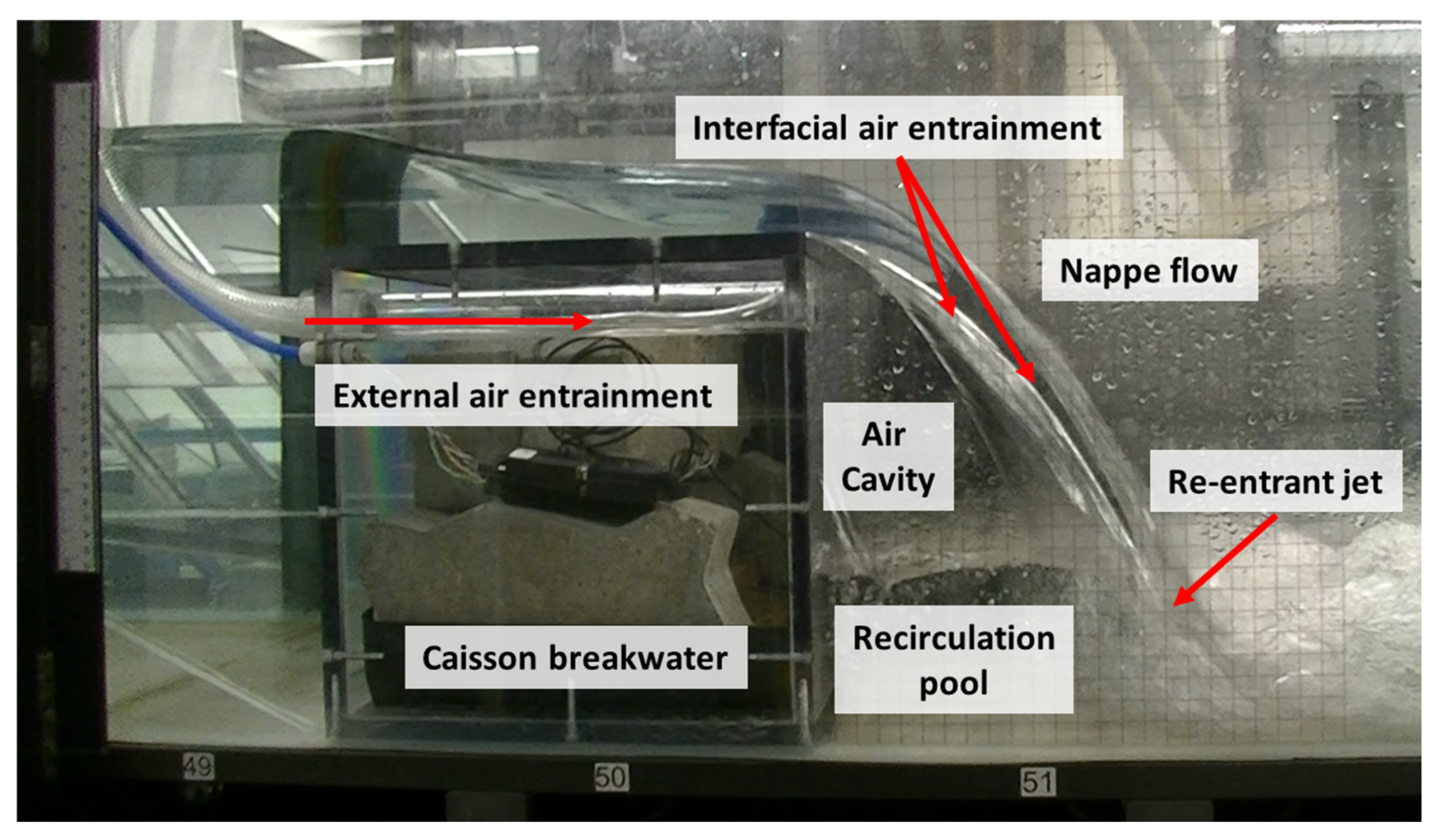
Figure 1. Air bubble entrainment along a cavity interface.
Jmse 12 01135 g001
Figure 2. Illustration of the effects of air cavity pressure and cavity water depth on a caisson breakwater.
Jmse 12 01135 g002
Figure 3. Visualization of independent (blue) and dependent (red) variables.
Jmse 12 01135 g003
Figure 4. Side view of the flume used in the experiment.
Jmse 12 01135 g004
Figure 5. Downstream face of the vertical caisson breakwater.
Jmse 12 01135 g005
Figure 6. Air cavity pressure ( p c ) and cavity water depth ( h c ) during overflow: (a) ventilated case. (b) non-ventilated case.
Jmse 12 01135 g006
Figure 7. Identification of points 1 and 2 for Bernoulli equation: view of actual setup.
Jmse 12 01135 g007
Figure 8. Different downstream flow regimes: (a) subcritical downstream. (b) supercritical downstream.
Jmse 12 01135 g008
Figure 9. Comparison of linear (left) and quadratic (right) regression models for predicting dimensionless air cavity pressure in subcritical downstream condition.
Jmse 12 01135 g009
Figure 10. Comparison of linear (left) and quadratic (right) regression models for predicting dimensionless air cavity pressure in supercritical downstream condition.
Jmse 12 01135 g010
Figure 11. Comparison of linear (left) and quadratic (right) regression models for predicting dimensionless air cavity pressure without Π 4 in supercritical downstream condition.
Jmse 12 01135 g011
Figure 12. Comparison of linear (left) and quadratic (right) regression models for predicting dimensionless cavity water depth in subcritical downstream condition.
Jmse 12 01135 g012
Figure 13. Comparison of linear (left) and quadratic (right) regression models for predicting dimensionless cavity water depth in supercritical downstream condition.
Jmse 12 01135 g013
Figure 14. Comparison of linear (left) and quadratic (right) regression models for predicting dimensionless cavity water depth without Π 4 in supercritical downstream condition.
Jmse 12 01135 g014
Table 1. Independent and dependent variables in the experiment.
VariablesValuesUnit
Independent variablesUpstream depth relative to crest h u p 0.055, 0.061, 0.065, 0.083, and 0.101
(5 cases)
[m]
Caisson breakwater height h b 0.300 (1 case)[m]
Downstream flume outlet height h o 0.100, 0.125, and 0.150 (3 cases)[m]
Cavity ventilation conditionVentilated or Non-ventilated (2 cases)[ ]
Dependent variablesAir cavity pressure p c Measured[Pa]
Cavity water depth h t Measured[m]
Table 2. Dimensionless parameters for air cavity pressure and cavity water depth.
Dependent VariableDownstream
Flow Regime
Dimensionless Equation
Equation Form Π 1 Π 2 Π 3 Π 4
Air cavity pressure  p c Subcritical(4) p c ρ g h u p h u p h b F r d h o h b
Supercritical(4) p c ρ g h u p h u p h b F r d h o h b
(5) p c ρ g h u p h u p h b F r d
Cavity water depth h t Subcritical(4) h t h b h u p h b F r d h o h b
Supercritical(4) h t h b h u p h b F r d h o h b
(5) h t h b h u p h b F r d
Table 3. Comparative analysis of air cavity pressure, cavity water depth, downstream Froude number, and air flow rate across different downstream flow regimes.
Independent
Variables
Ventilated CaseNon-Ventilated CaseDownstream Regime
h u p
[m]
h b
[m]
h w
[m]
p ¯ c , v
[Pa]
h ¯ c , v
[m]
h d , v
[m]
F r d , v R e a i r Q a i r
[lpm]
p ¯ c , n
[Pa]
h ¯ c , n
[m]
h d , n
[m]
F r d , n
0.0550.3000.100−0.010.0860.0700.329265646.3−28.880.0950.0700.329Subcritical
0.0610.3000.100−0.040.0880.0700.410266346.4−34.020.0930.0670.410Subcritical
0.0650.3000.100−0.040.0880.0640.488266446.4−38.120.0930.0640.488Subcritical
0.0830.3000.100−6.700.0930.0137.876376165.5−61.270.1080.0137.876Supercritical
0.1010.3000.100−21.080.1080.01310.572541994.5−94.090.1210.01310.572Supercritical
0.0550.3000.125−0.020.1120.1020.188265946.4−34.270.1220.1020.188Subcritical
0.0610.3000.125−0.050.1100.1000.240266546.5−38.370.1220.0950.240Subcritical
0.0650.3000.125−0.070.1100.0890.295266946.5−41.000.1230.0890.295Subcritical
0.0830.3000.125−5.310.1050.0137.876356062.1−55.440.1140.0137.876Supercritical
0.1010.3000.125−24.210.1100.01310.572571699.7−76.400.1210.01310.572Supercritical
0.0550.3000.150−0.020.1410.1330.125265846.3−63.810.1590.1400.125Subcritical
0.0610.3000.1500.920.1370.1200.170246443.0−64.780.1520.1210.170Subcritical
0.0650.3000.150−0.050.1380.1140.202266546.5−72.290.1560.1140.202Subcritical
0.0830.3000.150−3.550.1370.1020.348328757.3−95.700.1590.1020.348Subcritical
0.1010.3000.150−18.610.1330.0890.572517290.2−114.40.1520.0890.572Subcritical
Table 4. Final dimensionless equation for air cavity pressure in the subcritical downstream scenario.
Dimensionless ParametersDimensionless Equation (Subcritical Downstream)
Π 1 Π 2 Π 3 Π 4
p c ρ g h u p h u p h b F r d h o h b Π 1 = β 0 + β 1 Π 2 + β 2 Π 3 + β 3 Π 4 + β 4 Π 2 2 + β 5 Π 2 Π 3 + β 6 Π 2 Π 4 + β 7 Π 3 2 + β 8 Π 3 Π 4 + β 9 Π 4 2
Goodness of fitCoefficientsVentilated/
non-ventilated
CoefficientsVentilated/
non-ventilated
IndicatorVentilated/
non-ventilated
β 0 −0.095/−0.137 β 5 1.343/−0.699
β 1 −0.611/2.440 β 6 3.026/−2.400
R0.984/0.995 β 2 0.324/−1.043 β 7 −0.266/0.397
R-squared0.969/0.989 β 3 0.542/0.150 β 8 −1.051/2.523
RMSE0.001/0.003 β 4 −2.660/−3.669 β 9 −1.011/−0.697
Table 5. Final dimensionless equation for air cavity pressure in the supercritical downstream scenario.
Dimensionless ParametersDimensionless Equation (Supercritical Downstream)
Π 1 Π 2 Π 3 Π 4
p c ρ g h u p h u p h b F r d h o h b Π 1 = β 0 + β 1 Π 2 + β 2 Π 3 + β 3 Π 4 + β 4 Π 2 2 + β 5 Π 2 Π 3 + β 6 Π 2 Π 4 + β 7 Π 3 2 + β 8 Π 3 Π 4 + β 9 Π 4 2
Goodness of fitCoefficientsVentilated/
non-ventilated
CoefficientsVentilated/
non-ventilated
IndicatorVentilated/
non-ventilated
β 0 −0.010/−0.045 β 5 0.000/0.000
β 1 0.000/0.000 β 6 0.012/−0.018
R0.985/0.971 β 2 0.000/0.000 β 7 0.000/−0.001
R-squared0.971/0.942 β 3 0.122/−0.184 β 8 −0.022/0.048
RMSE0.001/0.002 β 4 0.000/0.000 β 9 0.091/−0.138
Table 6. Reduced dimensionless equation for air cavity pressure in the supercritical downstream scenario without Π 2 .
Dimensionless ParametersDimensionless Equation without Π 2 (Supercritical Downstream)
Π 1 Π 2 Π 3 Π 4
p c ρ g h u p F r d h o h b Π 1 = f ( Π 3 , Π 4 ) = β 0 + β 1 Π 3 + β 2 Π 4 + β 3 Π 3 2 + β 4 Π 3 Π 4 + β 5 Π 4 2
Goodness of fitCoefficientsVentilated/
non-ventilated
CoefficientsVentilated/
non-ventilated
IndicatorVentilated/
non-ventilated
β 0 −0.010/−0.045 β 3 0.000/−0.010
β 1 0.000/0.000 β 4 −0.022/−0.048
R0.985/0.971 β 2 0.122/−0.185 β 5 0.092/−0.139
R-squared0.971/0.942
RMSE0.001/0.002
Table 7. Final dimensionless equation for cavity water depth in the subcritical downstream scenario.
Dimensionless ParametersDimensionless Equation (Subcritical Downstream)
Π 1 Π 2 Π 3 Π 4
h c h b h u p h b F r d h o h b Π 1 = β 0 + β 1 Π 2 + β 2 Π 3 + β 3 Π 4
Goodness of fitCoefficientsVentilated/non-ventilated
IndicatorVentilated/
non-ventilated
β 0 −0.221/−0.153
β 1 −0.781/−0.257
R0.984/0.995 β 2 0.265/0.087
R-squared0.969/0.989 β 3 1.708/1.510
RMSE0.001/0.003
Table 8. Final dimensionless equation for cavity water depth in the supercritical downstream scenario.
Dimensionless ParametersDimensionless Equation (Supercritical Downstream)
Π 1 Π 2 Π 3 Π 4
h c h b h u p h b F r d h o h b Π 1 = β 0 + β 1 Π 2 + β 2 Π 3 + β 3 Π 4 + β 4 Π 2 2 + β 5 Π 2 Π 3 + β 6 Π 2 Π 4 + β 7 Π 3 2 + β 8 Π 3 Π 4 + β 9 Π 4 2
Goodness of fitCoefficientsVentilated/-ventilatedCoefficientsVentilated/-ventilated
IndicatorVentilated/-ventilated β 0 −0.254/−0.098 β 5 0.000/0.000
β 1 0.000/0.000 β 6 0.264/0.225
R0.978/0.983 β 2 0.001/0.000 β 7 0.010/0.009
R-squared0.957/0.966 β 3 2.704/2.307 β 8 −0.460/−0.403
RMSE0.008/0.007 β 4 0.000/0.000 β 9 2.028/1.730
Table 9. Reduced dimensionless equations for cavity water depth in the supercritical downstream scenario without Π 2 .
Dimensionless ParametersDimensionless Equation without Π 2 (Supercritical Downstream)
Π 1 Π 2 Π 3 Π 4
h c h b F r d h o h b Π 1 = f ( Π 3 , Π 4 ) = β 0 + β 1 Π 3 + β 2 Π 4 + β 3 Π 3 2 + β 4 Π 3 Π 4 + β 5 Π 4 2
Goodness of fitCoefficientsVentilated/
non-ventilated
CoefficientsVentilated/
non-ventilated
IndicatorVentilated/
non-ventilated
β 0 −0.252/−0.097 β 3 0.010/0.009
β 1 0.001/0.000 β 4 −0.455/−0.398
R0.978/0.983 β 2 2.721/2.321 β 5 2.041/1.741
R-squared0.957/0.966
RMSE0.008/0.007
Table 10. Froude, Weber, and Reynolds numbers at the brink of the caisson breakwater for different independent variables.
Independent VariableDimensionless NumbersAir Cavity Pressure p c [Pa]Cavity Water Depth h c [m]
h u p [m] h b [m] h w [m] F r b r W e b r R e b r VentilatedNon-
Ventilated
VentilatedNon-
Ventilated
0.0550.3000.1001.65420919,042−0.01−28.880.0860.095
0.0610.3000.1001.65425722,241−0.04−34.020.0880.093
0.0650.3000.1001.65429224,464−0.04−38.120.0880.093
0.0830.3000.1001.65447635,300−6.70−61.270.0930.108
0.1010.3000.1001.65470547,385−21.08−94.090.1080.121
0.0550.3000.1251.65420919,042−0.02−34.270.1120.122
0.0610.3000.1251.65425722,241−0.05−38.370.1100.122
0.0650.3000.1251.65429224,464−0.07−41.000.1100.123
0.0830.3000.1251.65447635300−5.31−55.440.1050.114
0.1010.3000.1251.65470547,385−24.21−76.400.1100.121
0.0550.3000.1501.65420919,042−0.02−63.810.1410.159
0.0610.3000.1501.65425722,2410.92−64.780.1370.152
0.0650.3000.1501.65429224,464−0.05−72.290.1380.156
0.0830.3000.1501.65447635,300−3.55−95.700.1370.159
0.1010.3000.1501.65470547385−18.61−114.350.1330.152
Disclaimer/Publisher’s Note: The statements, opinions and data contained in all publications are solely those of the individual author(s) and contributor(s) and not of MDPI and/or the editor(s). MDPI and/or the editor(s) disclaim responsibility for any injury to people or property resulting from any ideas, methods, instructions or products referred to in the content.