Article

Upper Ocean Responses to Tropical Cyclone Mekunu (2018) in the Arabian Sea

1
College of Oceanic and Atmospheric Sciences, Ocean University of China, Qingdao 266100, China
2
Yazhou Bay Innovation Institute, Hainan Tropical Ocean University, Sanya 572025, China
3
National Ocean Technology Center, Tianjin 300112, China
*
Author to whom correspondence should be addressed.
J. Mar. Sci. Eng. 2024, 12(7), 1177; https://doi.org/10.3390/jmse12071177
Submission received: 9 June 2024 / Revised: 4 July 2024 / Accepted: 11 July 2024 / Published: 13 July 2024
(This article belongs to the Section Physical Oceanography)

Abstract

:
Based on Argo observations and a coupled atmosphere–ocean–wave model, the upper ocean responses to the tropical cyclone (TC) Mekunu (2018) were investigated, and the role of a pre-existing cold eddy in modulating the temperature response to TC Mekunu was quantified by employing numerical experiments. With TC Mekunu’s passage, the mixed layer depth (MLD) on both sides of its track significantly deepened. Moreover, two cold patches (<26 °C) occurred, where the maximum cooling of the mixed layer temperature (MLT) reached 6.62 °C and 6.44 °C. Both the MLD and MLT changes exhibited a notable rightward bias. However, the changes in the mixed layer salinity (MLS) were more complex. At the early stage, the MLS on both sides of the track increased by approximately 0.5 psu. When TC Mekunu made landfall, the MLS change around the track was asymmetric. Significantly, a cold eddy pre-existed where the second cold patch emerged, and this eddy was intensified after TC Mekunu’s passage, with an average sea surface height reduction of approximately 2.7 cm. By employing the stand-alone ocean model, the numerical experimental results demonstrated that the pre-existing cold eddy enhanced TC-induced MLT cooling by an average of approximately 0.41 °C due to steeper temperature stratification at the base of mixed layer. Moreover, heat budget analysis indicated that the pre-existing cold eddy also enhanced subsurface temperature cooling mainly through zonal advection.

1. Introduction

The Indian Ocean is a basin with a high incidence of tropical cyclones (TCs). In contrast to the single TC season in other basins, TCs in the Arabian Sea (AS) and the Bay of Bengal (BoB) mainly occur during April–May and October–November months. Compared to those in the BoB, TCs occur slightly less frequently over the AS. This is due to the higher sea surface temperature (SST) in the BoB, which is favorable for TC genesis [1,2]. It has been reported that the frequency of intense TCs in the AS has increased in recent years within the context of global warming [3,4,5].
TCs with strong winds always impel the ocean to generate notable dynamic responses. Typically, stronger near-inertial currents are observed on the right side of TC tracks in the Northern Hemisphere. This occurs as a consequence of the resonance effect that results from TC winds rotating in the same direction as the near-inertial currents, which leads to a further acceleration of the near-inertial currents [6]. After TC passage, these currents propagate downward into the ocean subsurface as near-inertial internal waves [7,8,9], the vertical shear of which contribute to enhancing current shear instability, triggering diapycnal mixing [6].
Accompanied by dynamic processes, TCs always induce notable thermodynamic responses. During the forced stage, the most significant thermodynamic response is SST cooling. In the Northern Hemisphere, the spatial distribution of most TC-induced SST cooling is rightward-biased on account of the resonance effect of the local wind stress and near-inertial currents [6,10,11,12]. However, the maximum cooling also emerges on the left side in specific cases. For instance, the magnitude of SST cooling on the left side of the track of TC Orissa (1999) was greater because of the offshore transport of seawater [13]. There are three main dominant factors accounting for TC-induced SST cooling, namely vertical mixing, advection and heat exchange at the sea surface [14]. It has been previously demonstrated that vertical mixing associated with upwelling dominates TC-induced cooling wakes by approximately 70–80% [10,15], whereas the joint contribution of the remaining two factors is only approximately 20% [14,15,16]. However, the relative contributions of these three processes may vary considerably in different cases. Notably, mixing triggers decreases in the surface temperature as well as increases in the subsurface temperature, which is referred to as the “heat pump” effect [10,17,18]. During the relaxation stage, the increased surface heat input leads to stratification adjustment of seawater and a gradual return of the upper ocean temperature to its initial state, which usually takes a few to a dozen days [19,20,21].
Sea surface salinity (SSS) also significantly changes during the passage of TCs resulting from rainfall, evaporation, mixing, upwelling, and advection [22]. For instance, mooring buoy observations indicated that TC Jal (2010) induced a 1 psu increase in the SSS in the BoB [23], while TC Phailin (2013) caused a 2–3 psu increase in the SSS in the northwestern BoB [24,25]. The SSS response is also asymmetric because of the asymmetry of TC-induced vertical mixing and heavy precipitation [26].
The SST and SSS changes are also dependent on the attributes of TCs [11,27,28]. In general, TCs with low translation speed or strong intensity induce prominent SST cooling due to their longer forcing time or greater energy input to the upper ocean [29,30]. However, intense TCs do not necessarily induce greater SST cooling than weak TCs. For instance, although TC Phailin (2013, category 5) was much stronger than TC Hudhud (2014, category 4), the latter induced more rapid and intense SST cooling [31]. Moreover, the upwelling induced by strong or slow-moving TCs generally produces more SSS anomalies than that which is induced by weak or fast-moving TCs [32,33].
Additionally, the background ocean conditions also affect the ocean responses to TCs. Most TCs inevitably encounter mesoscale eddies during their life cycle [34,35,36,37]. In the western Pacific and the BoB, the interactions between TCs and mesoscale eddies have been extensively examined, with several landmark achievements. During the passage of TCs, the positive vorticity imported into the ocean can lead to changes in pre-existing eddies, including their strength and three-dimensional structure [38,39], and can even generate new cyclonic eddies [40]. Changes in eddies also significantly affect the magnitude of SST cooling through processes such as vertical advection, stirring, and mixing. Typically, cold eddies enhance TC-induced SST cooling, while warm eddies suppress TC-induced SST cooling [35,36,41]. However, Yablonsky and Ginis [42] reported that interactions between a warm eddy located on the right side of the TC track and the TC-induced cold wake could lead to greater SST cooling (in the Northern Hemisphere). In addition to modulating the magnitude of TC-induced SST cooling, pre-existing mesoscale eddies can alter the rightward-biased characteristics of SST cooling [41,43]. Nevertheless, the regulatory role of the interaction between intense TCs and mesoscale eddies has rarely been considered in the AS.
Although there has been a consensus on the modulatory role of mesoscale eddies in the upper ocean response to TCs, the specific dominant processes still deserve further investigation. Based on the coupled atmosphere–ocean–wave model, Prakash et al. [44] conducted three idealized numerical experiments to understand the interactions between TC Vardha (2016) and mesoscale eddies. Nevertheless, their case studies did not quantify the contributions of various physical processes to the temperature response. TC Mekunu (2018) was ranked, together with TC Phet (2010), as the strongest TC to impact the Arabian Peninsula, which passed over a cold eddy. In this study, on the basis of Argo observations and a coupled atmosphere–ocean–wave model with high-temporal and -spatial resolutions, the upper ocean responses to TC Mekunu were explored. In addition, by varying the ocean initial fields based on the stand-alone ocean model, we aimed to compare the heat budgets under the assumption of identical TC forcing to assess the relative importance of various physical processes to the modulated temperature response to TC Mekunu due to a pre-existing cold eddy.

2. Materials and Methods

2.1. Observations

The best track data for TCs in the Indian Ocean were obtained from the Indian Meteorological Department (IMD, https://mausam.imd.gov.in/, accessed on 2 May 2024). This dataset includes the location and intensity of each TC at 6-hour intervals during its lifetime.
TC Mekunu was an extremely severe cyclonic storm (ESCS) that occurred in the western AS in 2018. At 12:00 UTC on 21 May, a depression (D) system was generated at 58.5° E, 8.5° N. After its genesis, Mekunu moved northwestward and developed into a deep depression (DD) on the morning of 22 May. At 12:00 UTC on 22 May, Mekunu intensified into a cyclonic storm (CS). Due to the favorable atmospheric conditions and high SST, Mekunu intensified into a severe cyclonic storm (SCS) at 03:00 UTC and further into a very severe cyclonic storm (VSCS) at 09:00 UTC on 23 May, and it continued to move northwestward at approximately 10 km·h−1. At 03:00 UTC on 25 May, Mekunu further intensified into an ESCS, with a central air pressure of 964 hPa. On 26 May, TC Mekunu made landfall off the coast of the Dhofar Governorate in southern Oman, with the maximum wind speed of approximately 46 m·s−1 and three times the annual rainfall. Due to the terrain friction, TC Mekunu gradually weakened after landfall, and it finally weakened into a D system at 00:00 UTC on 27 May.
The Argo dataset was provided by the China Argo Real-time Data Center (http://www.argo.org.cn, accessed on 8 May 2024). This dataset had undergone quality control in real time or delayed before release.

2.2. Model Simulation
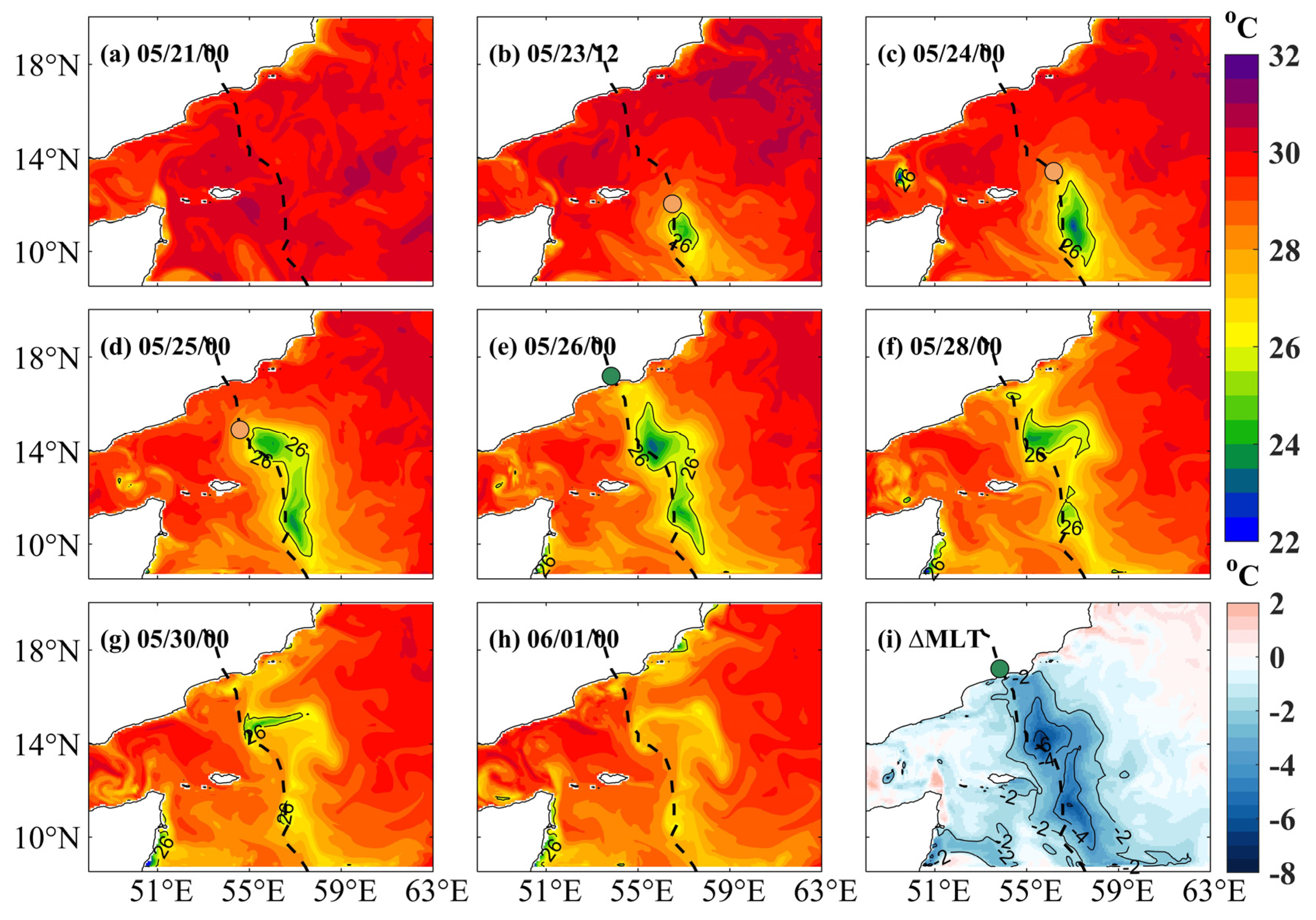
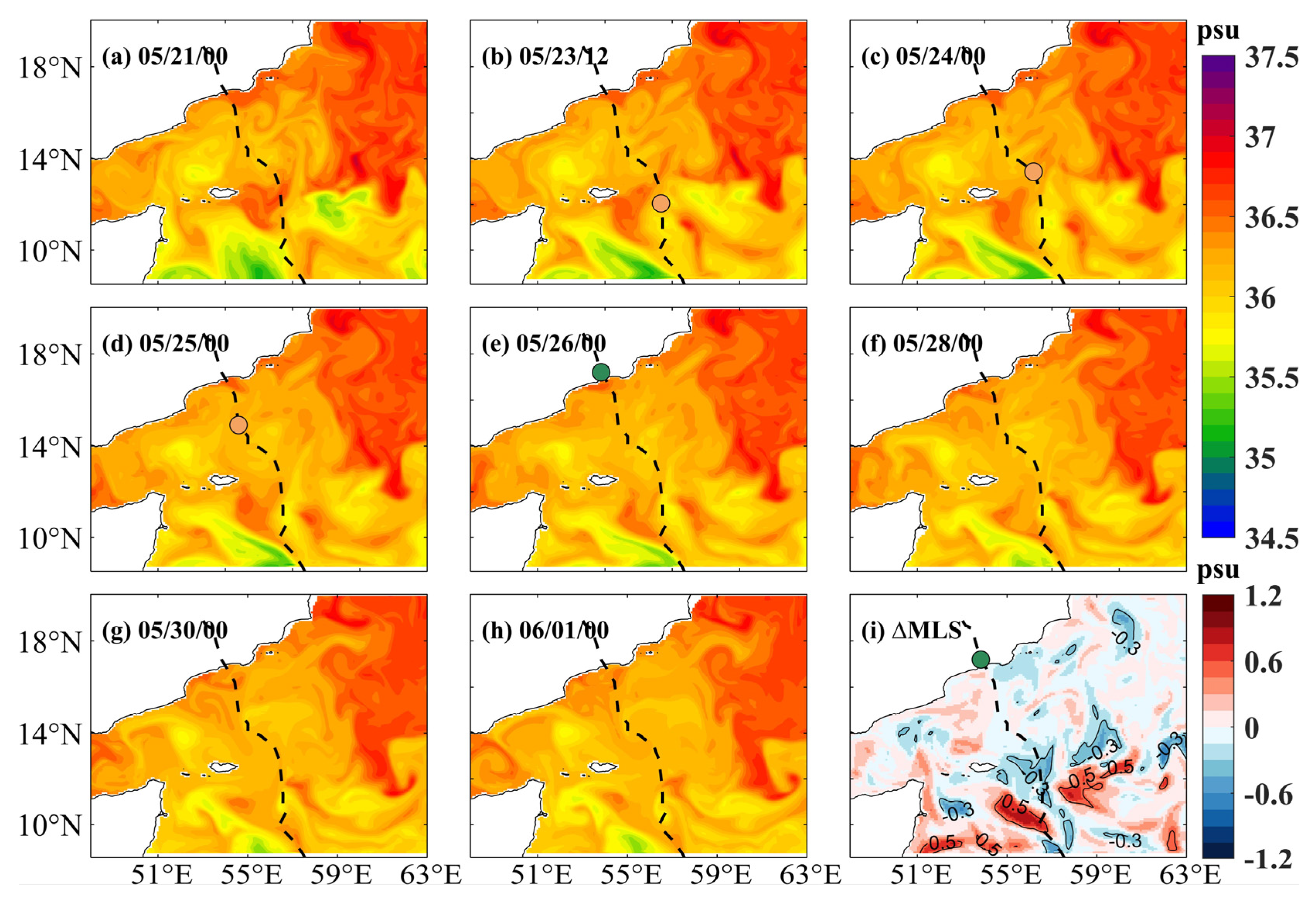
The coupled atmosphere–ocean–wave–sediment transport (COAWST) modeling system comprises several components, including the Weather Research and Forecasting (WRF), Regional Ocean Modeling System (ROMS), and Simulating Waves Nearshore (SWAN) models [45]. The transmission and exchange of different prognostic variables between these components are achieved by the Model Coupling Toolkit [46]. To date, the COAWST model has been popularly applied in the investigation of interactions between the upper ocean and TCs [44,47,48,49]. In this study, the atmosphere, ocean, and wave model components were coupled in the case of TC Mekunu. The coupled modeling was performed over the period from 20 May 2018 to 13 June 2018, and the data were stored at 6 h intervals.
As depicted as the black box in Figure 1, the WRF model domain covers the region between 43.6 and 64.3° E and 7.9 and 21.8° N, with a horizontal resolution of 9 km × 9 km. The WRF model was initialized with the Final Analysis (FNL) data from the National Centers for Environmental Prediction at 00:00 UTC on 20 May. Lateral boundary conditions were obtained from the FNL data at 6 h intervals. Vertically, the WRF model was discretized by 29 sigma levels. The specific parameter settings of the WRF model are listed in Table 1.
The ROMS model domain covers the region between 44.4 and 63.5° E and 8.7 and 20.9° N (i.e., the red box in Figure 1), with a horizontal resolution of 9 km × 9 km, which is sufficient to simulate the structure of mesoscale eddies and to examine the oceanic responses to TC Mekunu. The ROMS model was initialized with reanalysis data derived from the Hybrid Coordinate Ocean Model (HYCOM). The vertical resolution was set to 40 sigma levels, with the surface and bottom stretching parameters set to 4.7 and 0.1, respectively. The generic length scale scheme was selected to parameterize the vertical mixing process [50]. Chapman and Flather boundary conditions were imposed for free surface level and barotropic momentum, respectively. Radiation-nudging boundary condition was adopted for temperature, salinity, and the 3-dimensional currents. Gradient boundary condition was selected for mixing turbulent kinetic energy. Ocean bathymetry data were supported by ETOPO1 (1 arc-minute global relief data). The time step for both the WRF and ROMS models was set to 60 s. The SWAN model was used with a time step of 300 s. Variables were exchanged among these three model components at 600-s intervals.
Furthermore, numerical experiments were designed to examine the role of a pre-existing cold eddy in modulating the temperature response and its potential mechanisms. Given that TC-induced ocean responses are fed back to the TC in the coupled model and that upper ocean responses are in turn dependent on the attributes of TCs, two uncoupled simulations were performed by employing the stand-alone ROMS model in this study, i.e., a numerical simulation with a pre-existing cold eddy (EXP1) and a numerical simulation without a pre-existing cold eddy (EXP2). In both EXP1 and EXP2, the atmospheric forcing fields from 00:00 UTC on 20 May to 00:00 UTC on 13 June 2018 were obtained from the FNL data, including zonal and meridional components of 10 m wind, surface air pressure, relative humidity, shortwave and longwave radiation, 2 m air temperature, and precipitation rate. The ROMS model was initialized with the temperature, salinity, zonal velocity, meridional velocity, and sea surface height (SSH) values derived from the HYCOM reanalysis data. The difference between EXP1 and EXP2 is that the ROMS model in the former was initialized with the ocean state on 20 May 2018, while the ROMS model in the latter was initialized with the climatological ocean state on 20 May averaged from 2009 to 2018. The remaining parameter settings in the ROMS model were the same as those in the previous coupled simulation. This design successfully removed the pre-existing cold eddy, and the ocean (other than the eddy) maintained similar response characteristics, which would be discussed in detail in Section 3.3.2.

2.3. Mixed Layer

The oceanic mixed layer is a body of water located in the upper ocean that is approximately homogeneous in terms of the vertical temperature, salinity, density, and other properties. The mixed layer depth (MLD) is a vital physical parameter to characterize the mixed layer. In this study, the density difference method was adopted to calculate the MLD. To avoid the effects of anomalous thermal processes at the sea surface, a depth of 10 m is typically preferred. Based on the seawater state equation, the depth where the potential density difference from the value at the 10 m depth equals the threshold reported by de Boyer Montégut et al. [51] is denoted as the MLD, which can be expressed by Equation (1):
σ = σ T 10 0.2 , S 10 , P 0 σ T 10 , S 10 , P 0
where T10 and S10 are the temperature and salinity at the depth of 10 m, respectively, and P0 is the sea surface pressure. The mixed layer temperature (MLT) and mixed layer salinity (MLS) are taken as the average values of temperature and salinity above the bottom of the mixed layer, respectively.

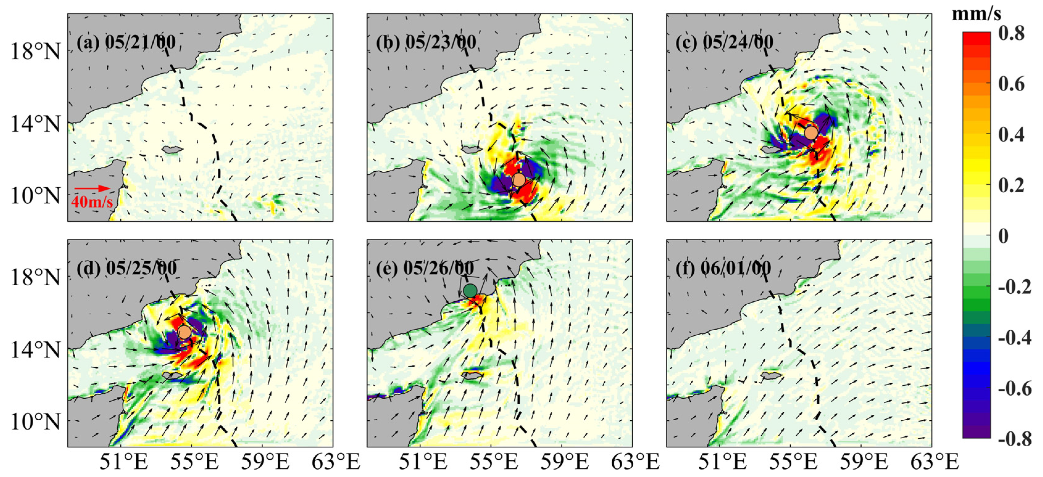
2.4. Ekman Pumping Velocity

The magnitude of TC-induced cooling is bound up with the Ekman pumping effect. The Ekman pumping velocity (EPV) is an important parameter to characterize the vertical motion of seawater, with a positive EPV value representing upwelling and a negative EPV value representing downwelling. It can be calculated using Equation (2):
E P V = x τ y ρ 0 f y τ x ρ 0 f
where ρ0 = 1025 kg·m−3 is the density of seawater, f is the Coriolis parameter, and τx and τy are the zonal and meridional components of the wind stress, respectively.

2.5. Heat Budget Equation

The heat budget equation is typically employed to quantify the relative importance of various physical processes to the temperature response to TCs. This is represented by Equation (3):
Tt = − TU+VTW + TDH + TDV + QS,
where Tt is the local rate of temperature change, TU+V is the horizontal advection term, TW is the vertical advection term, TDH is the horizontal diffusion term, TDV is the vertical diffusion term, and QS is the net heat flux term. In numerical simulations, the horizontal diffusion term is generally negligible because it is much smaller than the other terms, and the net heat flux term is integrated into the vertical diffusion term as the sea surface boundary condition.

3. Results and Discussion

3.1. Validation of the Coupled Model Simulations

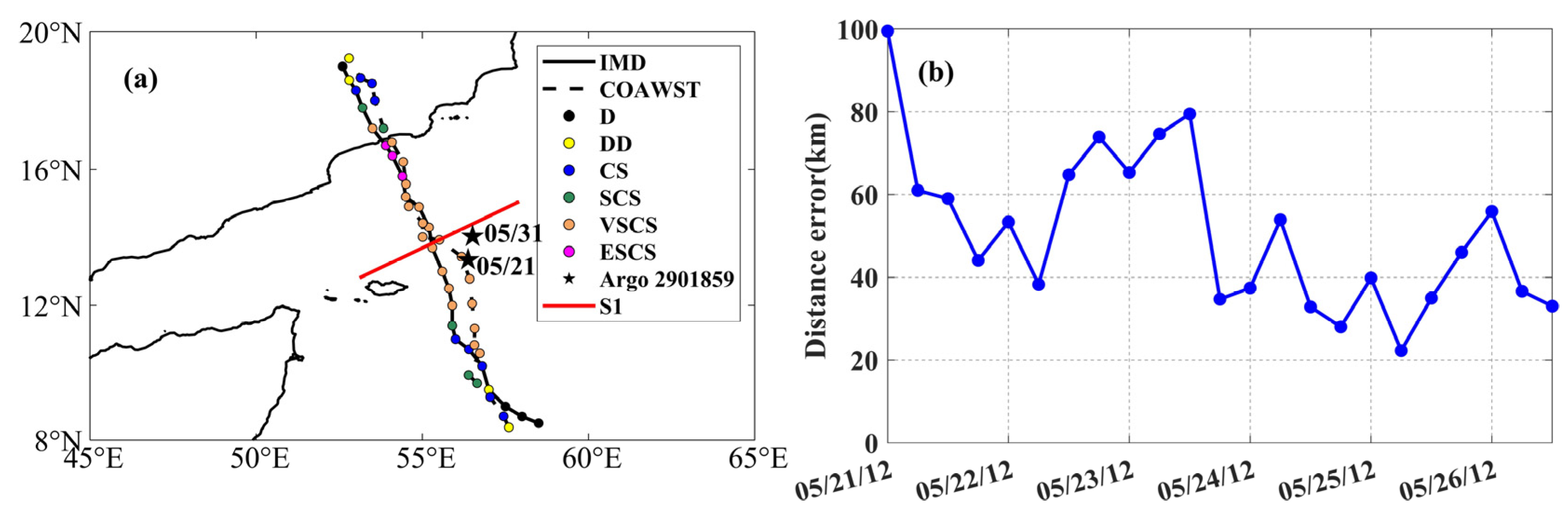
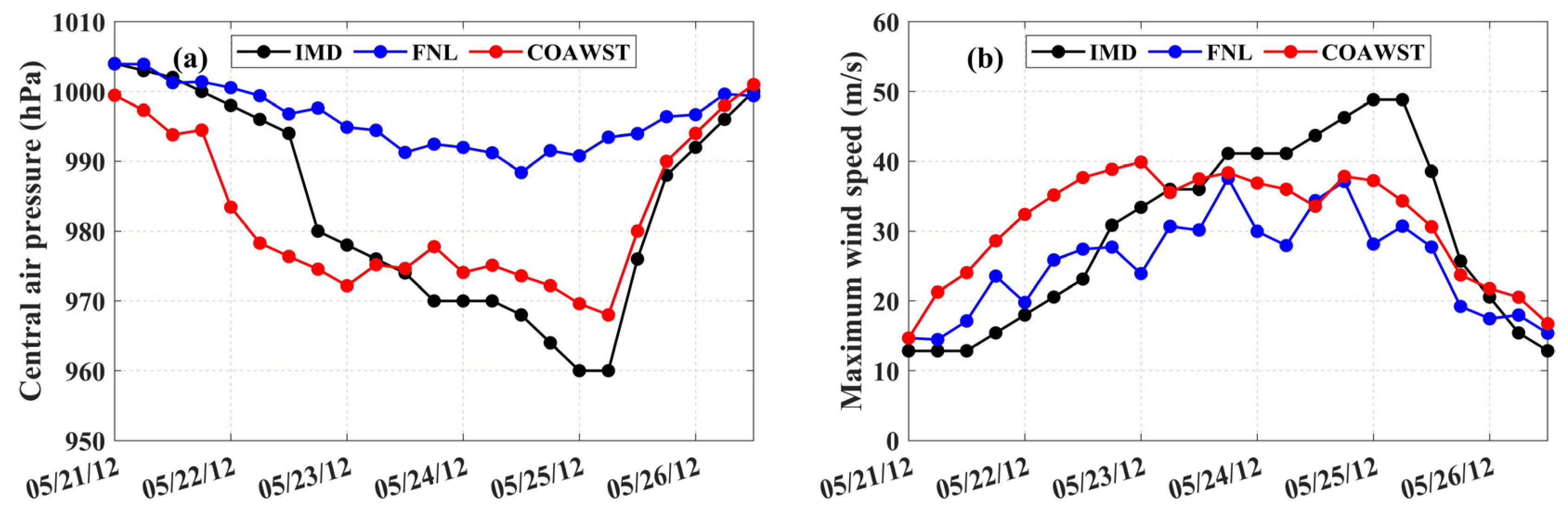
3.1.1. Track and Intensity of TC Mekunu

Figure 2a shows a comparison between the COAWST model simulated track of TC Mekunu and the IMD best track during the period from 12:00 UTC on 21 May 2018 to 00:00 UTC on 27 May 2018. It is discernible that the simulated track of TC Mekunu was essentially in line with the best track, but the simulated locations of the TC center slightly differed from the observations. As shown in Figure 2b, although the error was the largest at the time of TC Mekunu’s genesis (12:00 UTC on 21 May), reaching approximately 100 km, thereafter, the errors were less than 80 km. Generally, the mean error reached approximately 50 km. According to Liu et al. [52], these errors are due to the lower SST resulting from the coupling of atmosphere and ocean models and the negative feedback effect of the ocean, which could cause a corresponding change in the mesoscale structure of TCs.
The quality of COAWST model simulated central air pressure and maximum wind speed of TC Mekunu were related to that of the FNL data used as initial and boundary conditions for the WRF model. Compared to the IMD best estimates, the sea level pressure at the center of TC Mekunu derived from the FNL data was overall greater, with a maximum error of 33 hPa at 18:00 UTC on 25 May (Figure 3a). There were also some slight errors in the maximum wind speed from the FNL data (Figure 3b). The COAWST simulations overestimated the intensity of TC Mekunu at the early stage and underestimated its intensity at the late stage (Figure 3). The root-mean-squared errors of the simulated central air pressure and maximum wind speed reached approximately 8 hPa and 9 m·s−1, respectively.
In summary, the COAWST-simulated maximum intensity of TC Mekunu was weaker than that observed, with the maximum intensity reaching only the VSCS. The simulated track of TC Mekunu was essentially in line with the IMD best track. Generally, the COAWST model reproduced the genesis and development of TC Mekunu well.

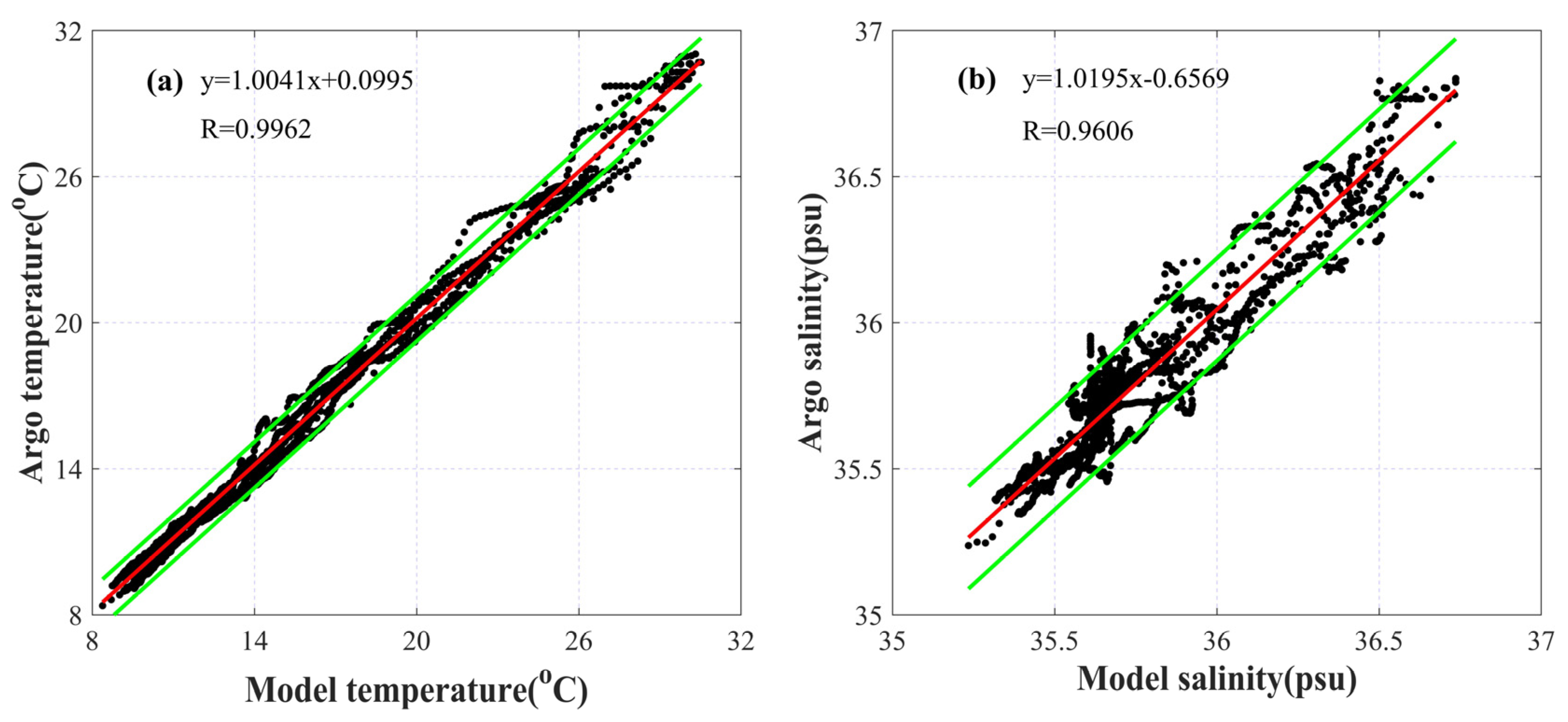
3.1.2. Ocean Thermohaline

While validating the ocean temperature and salinity simulated by the COAWST model, nine Argo profiles were used. Since the COAWST model outputs were stored at 6 h intervals, to match with the Argo observations better, the daily average temperature and salinity were first calculated and then interpolated to the depths measured by the Argo floats. Figure 4 displays the comparisons between the temperature and salinity simulated by the model and those measured by the Argo floats. Generally, the temperature simulated by the COAWST model matched the Argo observations well, with a correlation coefficient of 0.9962, while the salinity simulations exhibited some bias, with a correlation coefficient of 0.9606. The ocean temperature and salinity simulated by a high-resolution coupled atmosphere–ocean model were assessed by Thompson et al. [53]. They revealed that the root-mean-squared error of simulated ocean temperature varied within the range of 0.26–1.35 °C, and the root-mean-squared error of simulated ocean salinity mostly remained less than 0.15 psu. In evaluating the performance of the ROMS model, Yang et al. [54] indicated that the root-mean-squared errors were less than 1.5 °C for temperature and less than 1.5 psu for salinity. In this study, the root-mean-squared errors of the simulated ocean temperature and salinity reached approximately 0.51 °C and 0.09 psu, respectively, which were within acceptable error limits reported in the previous studies [53,54]. As a result, the COAWST model simulation results could be used in the following detailed analyses of upper ocean responses to TC Mekunu. Notably, the conclusions related to ocean temperature could be strongly bolstered by the fact that the temperature simulations closely matched the observations.

3.2. Ocean Responses in the Coupled Model

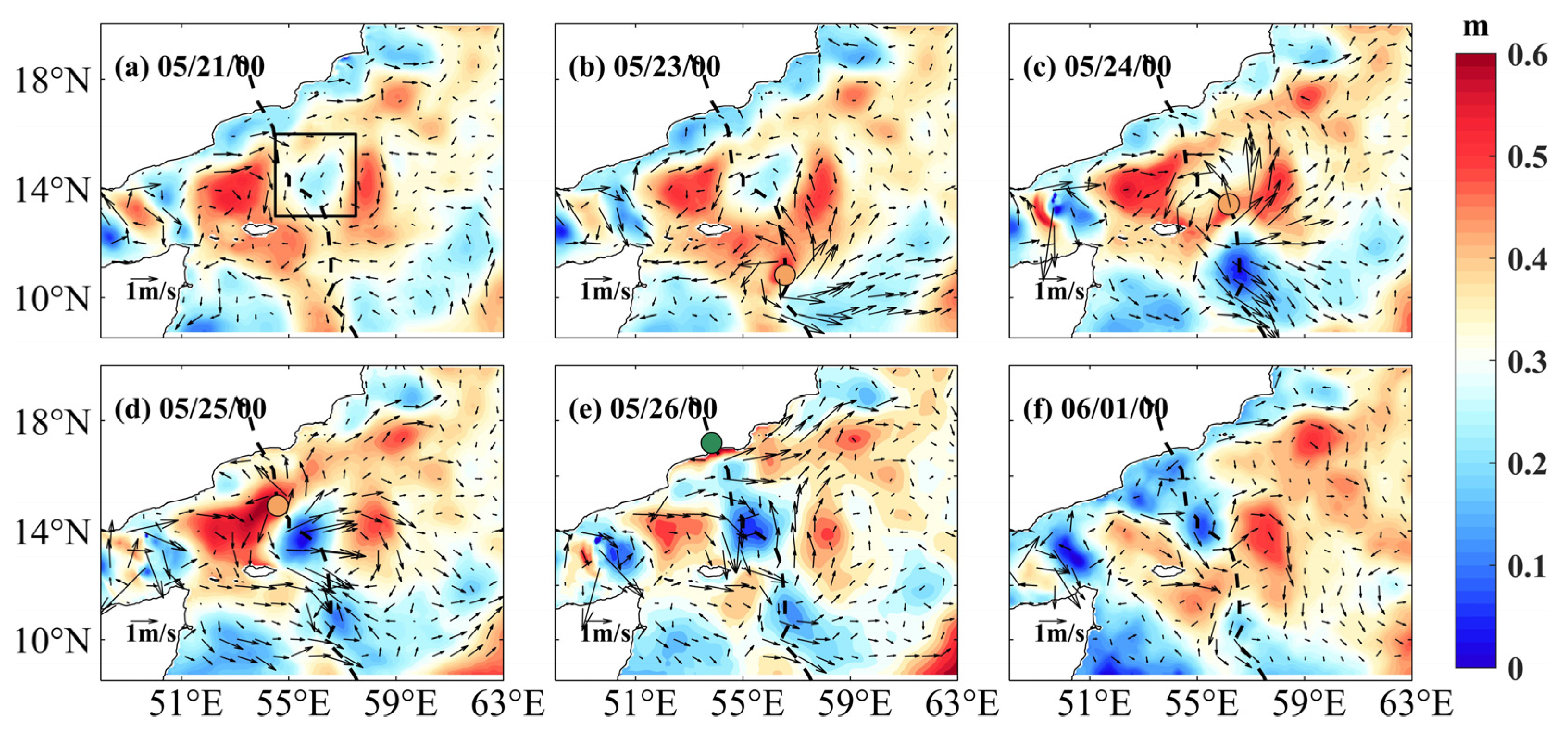
3.2.1. Surface Current Responses

TCs always cause notable dynamic responses in the upper ocean. In this study, a mesoscale cyclonic eddy pre-existed to the northeast of Socotra Island (Figure 5a). With TC Mekunu’s passage, the strong cyclonic wind fields enhanced the previous cyclonic current fields. Notably, the current velocity on the right side of the TC track was greater than that on the left side. Moreover, the local SSH in front of the TC Mekunu center increased because of the accumulation of seawater driven by wind stress, while the local SSH behind the TC Mekunu center decreased because of the loss of seawater (Figure 5b–d). At 00:00 UTC on 26 May, the northward surface currents along the southern coast of Oman remarkably intensified (Figure 5e). Five days after TC passage, the SSH in the local region (i.e., the black box in Figure 5a) where the cyclonic cold eddy pre-existed decreased by approximately 2.7 cm on average (Figure 5f).

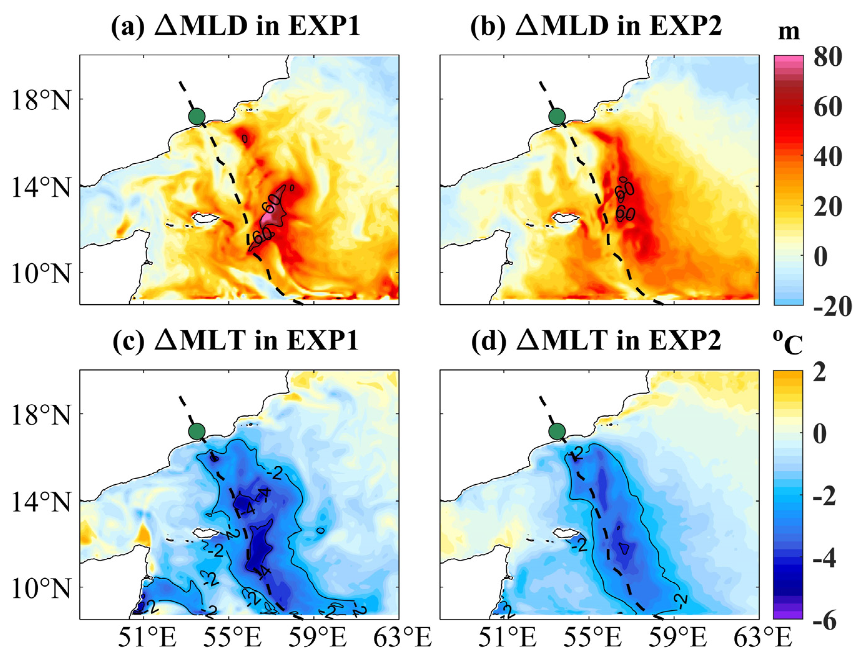
3.2.2. Mixed Layer Responses

The surface wind stress directly drives seawater. To characterize the vertical motion of seawater, the EPV was calculated using Equation (2). Before the passage of TC Mekunu, the magnitude of the EPV in the study region generally ranged from 10−3 to 10−2 mm·s−1 (Figure 6a). During TC Mekunu’s passage, the EPV notably responded to the forcing of wind stress with magnitudes up to 1 mm·s−1 (Figure 6b–e). Moreover, interphase convergent–divergent zones were formed around the vicinity of the TC Mekunu center, and the alternating upwelling and downwelling jointly referred to as inertial pumping [6] resulted in considerable vertical and turbulent mixing in the upper ocean, which could induce significant changes in the oceanic mixed layer [55,56]. At 00:00 UTC on 1 June, the study area was dominated by the summer monsoon wind system (Figure 6f).
The evolution of the MLD calculated by using Equation (1) is depicted in Figure 7. Before TC Mekunu’s passage, the MLD in the study region was relatively symmetrical, with the MLD around the vicinity of TC Mekunu reaching approximately 15 m (Figure 7a). During the passage of TC Mekunu, the MLD around the track significantly deepened, and the magnitude of MLD deepening exhibited a notable rightward bias (Figure 7b–e). At 00:00 UTC on 24 May, the rightward MLD deepened by approximately 20–70 m, while the magnitude of leftward MLD deepening was small at about 20–45 m (Figure 7c). At 00:00 UTC on 26 May, TC Mekunu made landfall, and the area affected by the TC further expanded, with the maximum MLD deepening in the coastal area reaching 98 m, occurring approximately 47 km to the right of the track (Figure 7i). Subsequently, the study region was gradually detached from TC Mekunu, and the MLD gradually became shallow (Figure 7f–h).
Due to intense Ekman pumping, subsurface water is pumped to the mixed layer, and the thermohaline structure of the mixed layer changes as a result. The MLT evolution is shown in Figure 8. Before the genesis of TC Mekunu, the MLT around its track exceeded 28.5 °C (Figure 8a). During the passage of TC Mekunu, the MLT around the track significantly dropped (Figure 8b–e). Similar to the signatures of the MLD patterns, the cooling magnitude and area on the right side of the track were greater than those on the left side, which is in line with the conclusion proposed by previous studies [10,15,16]. Moreover, the magnitude of MLT change reached an extreme value 1–2 days after TC Mekunu passed over the local ocean, suggesting that the effect of TC Mekunu on the mixed layer was delayed and persistent. Significantly, at 00:00 UTC on 24 May, a cold patch below 26 °C emerged to the right of the TC track, where the average MLT cooling was 4.33 °C, and the maximum MLT cooling reached 6.62 °C (56.90° E, 11.09° N) (Figure 8c). At 00:00 UTC on 26 May, a second cold patch below 26 °C emerged to the right of the track, the location of which coincided with the pre-existing cyclonic eddy mentioned above (Figure 8e). In the second cold patch, the average MLT cooling was 3.44 °C, and the maximum MLT cooling reached 6.44 °C (55.58° E, 14.03° N) (Figure 8i). After TC Mekunu moved away, the increased surface heat input led to stratification adjustment of seawater [57], and the MLT gradually recovered (Figure 8f–h). Significantly, the MLT of coastal seawater to the right of TC Mekunu’s track gradually dropped, and the cooling extended northward along the coastline (Figure 8f–h), which might be attributed to the effect of coastal upwelling. Five days after the departure of TC Mekunu, the MLT remained 1–3 °C lower than its initial state. Previous studies have revealed that the recovery time of cooling induced by TCs ranges from a few days to more than a month because it is closely dependent on the cooling magnitude, current field, and oceanic conditions (e.g., stratification, mesoscale eddies, and barrier layers) [28].
The MLS also significantly responded to TC Mekunu, and the MLS change was more complex than that in the MLT (Figure 9). At the early stage of TC Mekunu’s development (from 12:00 UTC on 23 May to 00:00 UTC on 24 May), the MLS on both sides of the track increased by approximately 0.5 psu, while the MLS along TC Mekunu’s track decreased by approximately 0.3 psu (Figure 9a–c). Later (from 00:00 UTC on 25 May to 00:00 UTC on 26 May), the MLS change around the vicinity of TC Mekunu center was relatively slight (Figure 9d,e). When TC Mekunu made landfall, the MLS differences in the coastal region were asymmetric because of the joint effect of the total advection and vertical diffusion terms, with the leftward MLS increasing and the rightward MLS decreasing by approximately 0.2 psu (Figure 9i). In contrast to that of the MLT, the MLS recovery trend in the study region was not obvious (Figure 9f–h), suggesting that the recovery time of the MLS was relatively longer. Girishkumar et al. [23] reported that the upper ocean salinity response could last about 10–12 days.

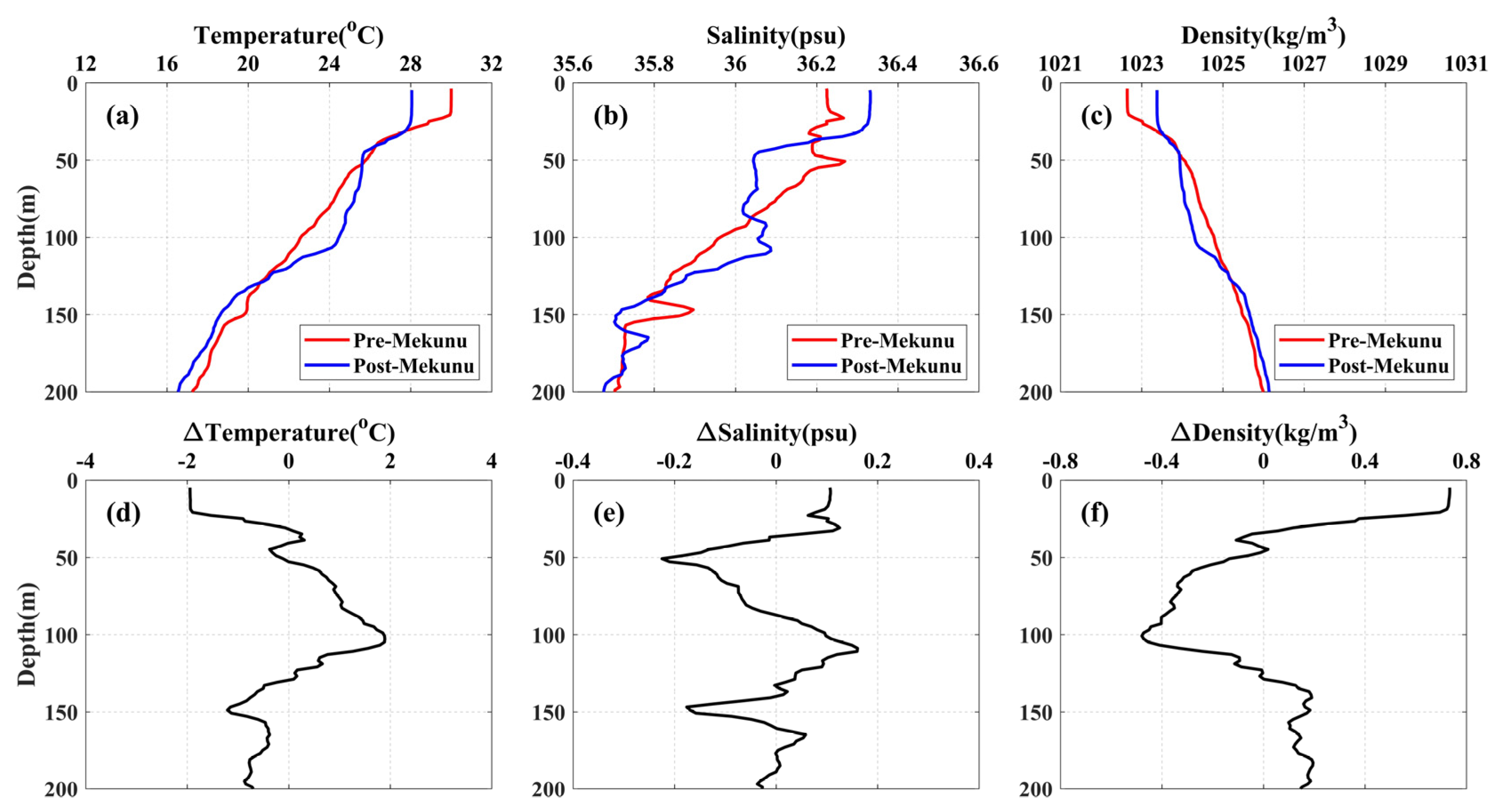
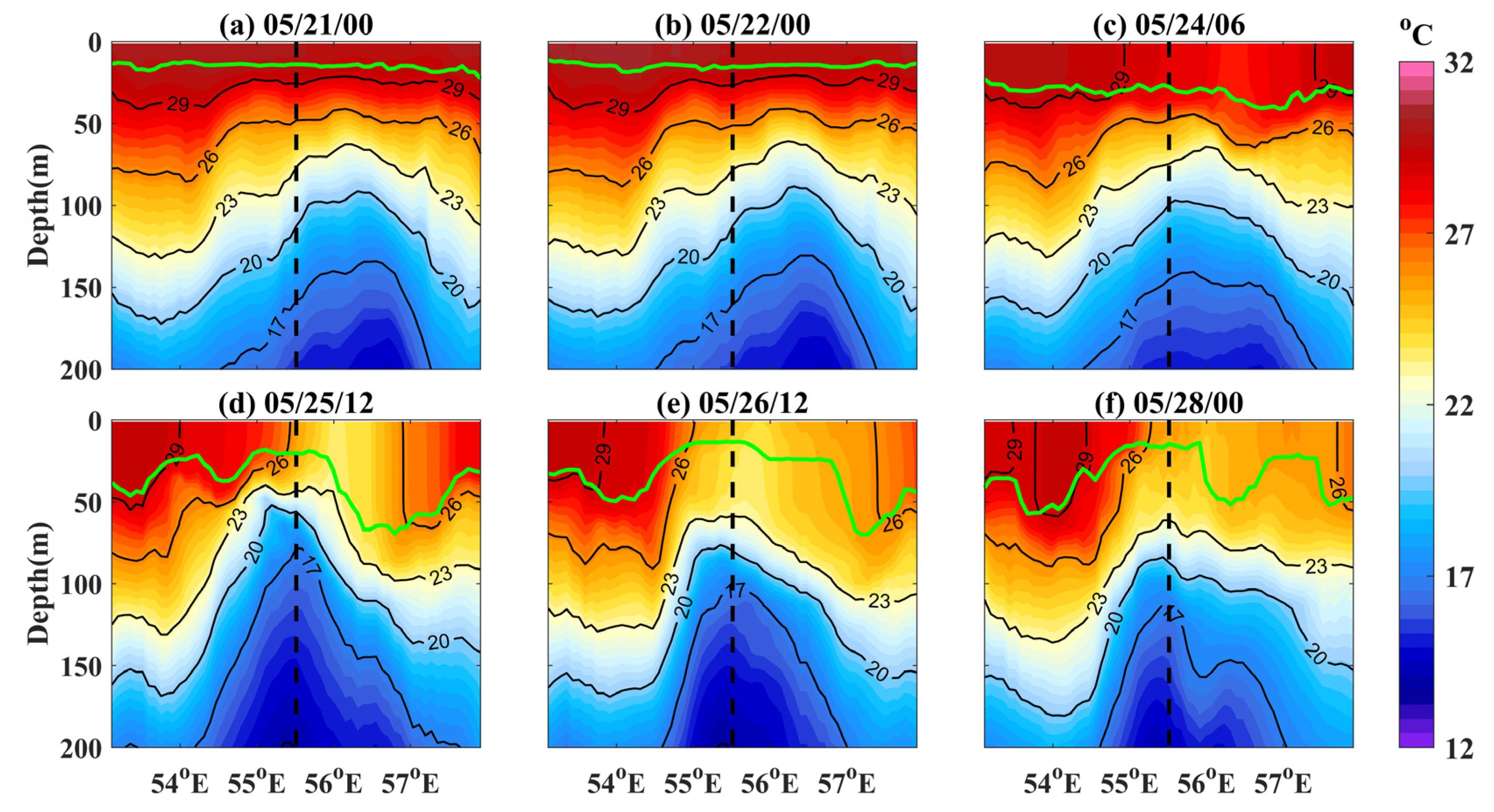
3.2.3. Subsurface Responses

The mixed layer responses induced by TC Mekunu were described in detail in Section 3.2.2. Moreover, TCs can also have a significant impact on the subsurface thermohaline structure [6,10,58].
Argo profile pairs are often used to examine the changes in ocean structure related to TCs [21,59,60,61]. The Argo float (number 2901859) successfully captured the characteristics of the upper ocean before and after TC Mekunu’s passage, the locations of which are depicted as black pentagrams in Figure 2a. Compared to the mixed layer on 21 May, the change in the mixed layer was manifested by an MLD deepening of 8.8 m, an MLT cooling of 2.0 °C and an MLS increase of 0.1 psu (Table 2). Cooling was also observed within a depth range of 130–200 m but with an overall smaller magnitude than that of the MLT. Notably, there was anomalous warming within the depth range of 50–130 m, with a maximum warming of approximately 1.9 °C at the depth of 100 m (Figure 10a,d), which was caused by entrained mixing at the base of mixed layer [10]. The salinity change in the subsurface layer was greater than that in the mixed layer. The salinity at depths of 35–87 m and 140–160 m decreased after TC Mekunu passed, with maximum decreases of 0.2 psu at a depth of 50 m and 0.17 psu at a depth of 150 m, while the salinity within a depth range of 88–140 m increased, with a maximum increase of 0.16 psu (Figure 10b,e). The temperature and salinity changes led to the density change. Density increase–decrease–increase changes were observed at depths of 0–30 m, 30–130 m, and 130–200 m, respectively, with the greatest density change occurring within a depth range of 0–30 m (Figure 10c,f).
Additionally, due to the lack of adequate in situ observations, we examined the subsurface responses along the S1 transect (i.e., the red line in Figure 2a) based on COAWST simulations. The center of the S1 transect coincided with the position of TC Mekunu center at 06:00 UTC on 24 May, which was located in the pre-existing cold eddy mentioned above. The evolution of the vertical temperature along the S1 transect is shown in Figure 11. Before TC Mekunu’s passage, the MLD along the S1 transect was uniformly distributed, with MLDs of approximately 15 m. However, in the subsurface layer, there was a mass of warm water to the left of TC Mekunu center, whereas the temperature was relatively much lower on the right (Figure 11a,b). When TC Mekunu reached the center of the S1 transect, the MLD along the S1 transect remarkably deepened, and the 29 °C isotherm was elevated to the sea surface within 80 km to the left and 200 km to the right of the TC Mekunu center (Figure 11c). Generally, the subsurface temperature within 120 km to the left of the TC Mekunu center decreased by approximately 1 °C. Even though TC Mekunu passed over the S1 transect, the upper ocean continued to respond. As evident from Figure 11d, the MLD significantly deepened and exhibited a rightward bias. Moreover, the oceanic isotherm above 200 m was significantly lifted on account of TC-induced upwelling, and the cold water on the right side gradually moved to the left side. As a consequence, contrary to the rightward bias in MLT cooling, the subsurface cooling within 150 km to the left of the TC Mekunu center was more prominent, with a magnitude of approximately 5.5 °C (Figure 11e). Subsequently, the ocean temperature gradually recovered (Figure 11f).

3.3. Role of the Pre-Existing Cold Eddy

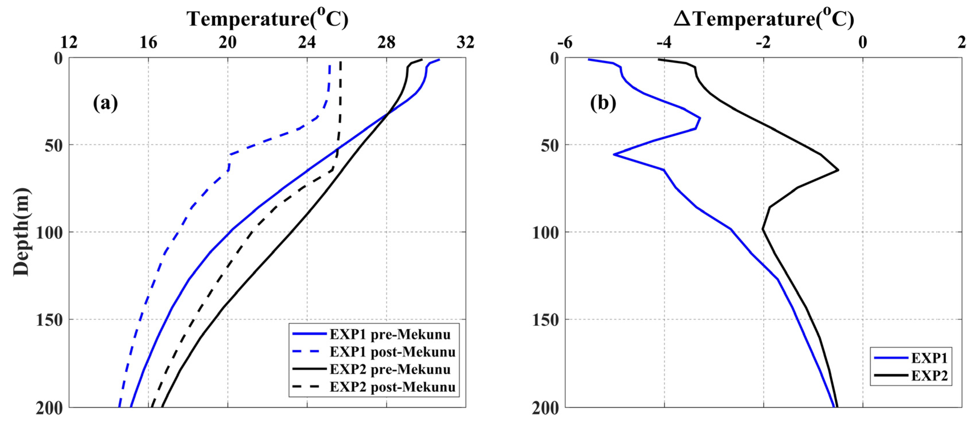
3.3.1. Initial Ocean Conditions

Oceanic mesoscale eddies may remarkably affect the magnitude and spatial distribution of TC-induced SST cooling [35,36,41,62]. However, the role of mesoscale eddies still remains to be quantified. TC Mekunu encountered a pre-existing cold eddy, and the pattern of the MLT response simulated by the COAWST model indicated a cold patch associated with this cold eddy. Two numerical experiments were designed to quantify the specific contribution of the pre-existing cold eddy to temperature cooling induced by TC Mekunu by using the stand-alone ROMS model, which did not consider the feedback effects of the ocean on the atmosphere.
Figure 12 shows the SSH, MLD, and depth of the 26 °C isotherm (D26) before TC Mekunu’s passage in EXP1 and EXP2. The region (54.5–57.5° E, 13–16° N, i.e., the black box in Figure 12) is referred to as region C, which is also the area of greatest focus in this section. Evidently, before the genesis of TC Mekunu, region C in EXP1 was characterized by lower SSH and shallower MLD and D26 values than those in EXP2 (Figure 12 and Table 3), as reported in a previous study [63]. Therefore, the SSH, MLD, and D26 patterns before the genesis of TC Mekunu reveal that the pre-existing cold eddy was effectively attenuated or even removed in EXP2.

3.3.2. Ocean Responses in the Uncoupled Model

The mixed layer responses within the study region related to TC Mekunu were examined in the two uncoupled experiments. As presented in Figure 13a,c, compared with the MLD and MLT responses simulated by the COAWST model, the results simulated in the uncoupled EXP1 were slightly smaller in terms of the magnitude of MLD deepening and MLT cooling induced by TC Mekunu. Nevertheless, the spatial distribution of the mixed layer responses to TC Mekunu in EXP1 exhibited a similar pattern to that of the coupled results. That is, EXP1 successfully reproduced the rightward bias in MLD deepening and MLT cooling, and the MLT cooling exhibited a multicore structure. Compared to the results in EXP1, the MLD response to TC Mekunu was also rightward-biased in EXP2, while the magnitude of MLD deepening was slightly smaller (Figure 13b). Specifically, MLT cooling in EXP2 exhibited a more homogeneous strip-like pattern (Figure 13d).
To further understand the modulatory role of the pre-existing cold eddy in determining the mixed layer responses, the evolution of the MLD and MLT within region C in the two experiments is investigated here. On average, the MLD deepening caused by TC Mekunu in EXP1 was only about 27 m, while the MLD deepening in EXP2 reached about 33 m. This suggests that this pre-existing cold eddy suppressed TC-induced MLD deepening. The average MLT cooling in region C reached maximum values of 3.01 °C in EXP1 and 2.60 °C in EXP2. The maximum MLT cooling was approximately 5.02°C in EXP1, occurring at 55.58° E, 14.03° N, which is denoted as Position 1 (P1) in the following, whereas the maximum MLT cooling at P1 in EXP2 reached only approximately 3.50 °C. In summary, the pre-existing cold eddy enhanced TC-induced MLT cooling, with an average increase of approximately 0.41 °C in region C and a maximum increase of approximately 1.52 °C at P1, which is consistent with previous studies [36,64].
Given that there was a significant MLT change at P1 within region C in the two experiments, the characteristics of the ocean vertical temperature above 200 m at P1 in EXP1 and EXP2 were examined and compared before and after TC Mekunu’s passage (Figure 14). On 20 May, the MLDs at P1 in EXP1 and EXP2 were approximately 15 m and 18 m, respectively. Notably, the temperature gradient above 100 m in EXP1 was steeper than that in EXP2 (Figure 14a). As noted in a previous study, steeper temperature stratification at the base of mixed layer favors the induction of greater cooling [15]. After the passage of TC Mekunu, remarkable cooling was observed in the ocean above 200 m at P1 in EXP1 and EXP2 (Figure 14b). Interestingly, no warming was observed. This might have occurred because the cooling effect of upwelling exceeds the warming effect of vertical mixing [6]. Moreover, the cooling in EXP1 was greater than that in EXP2 overall (Figure 14b). This suggests that the pre-existing cold eddy enhanced not only MLT cooling but also subsurface cooling.

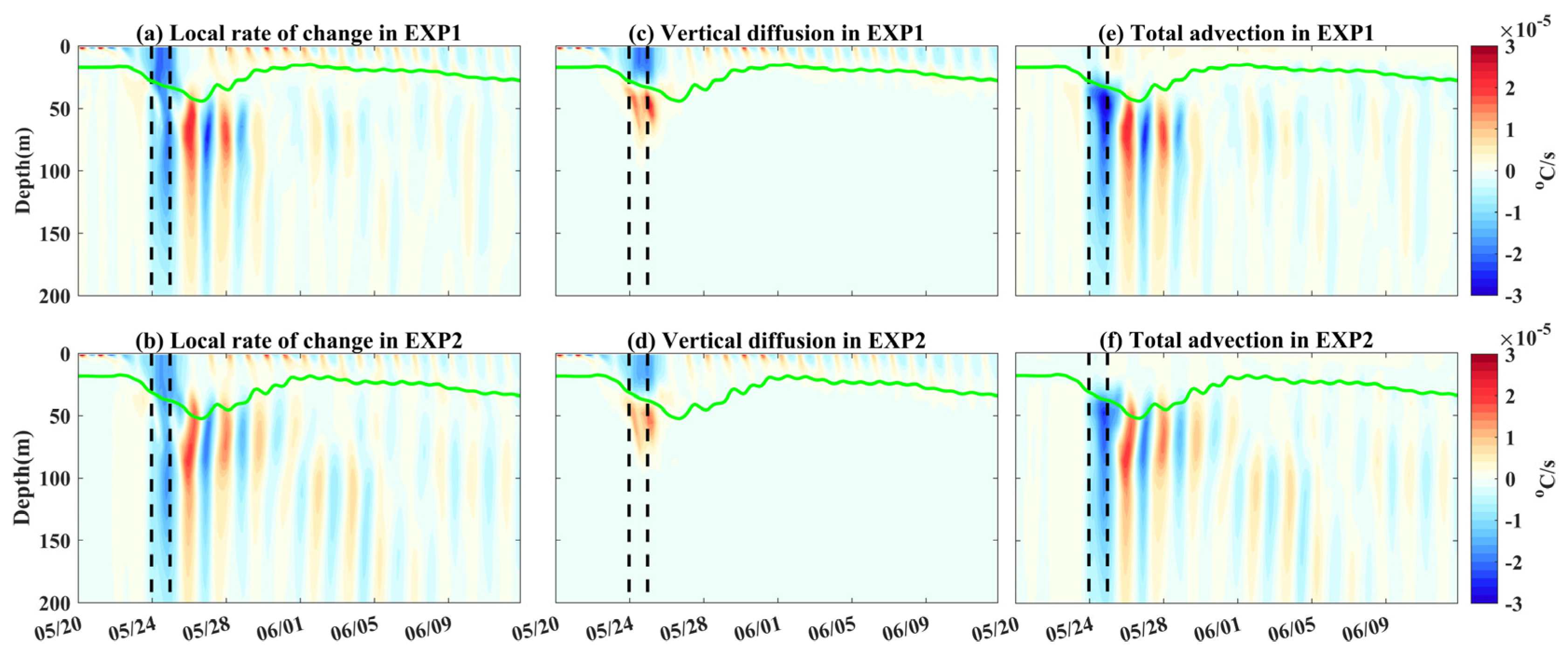
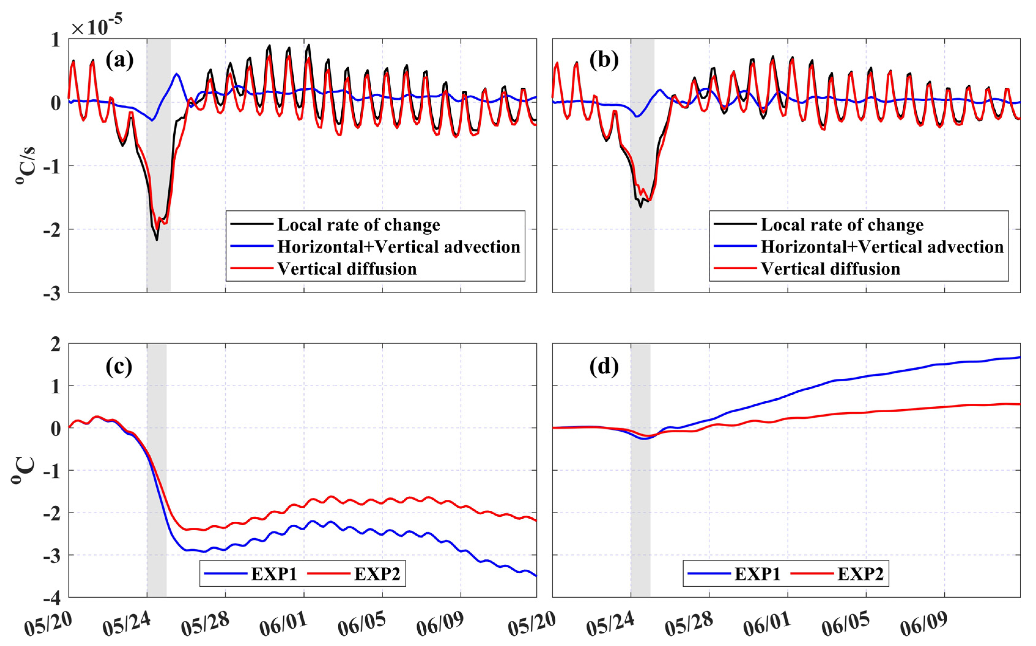
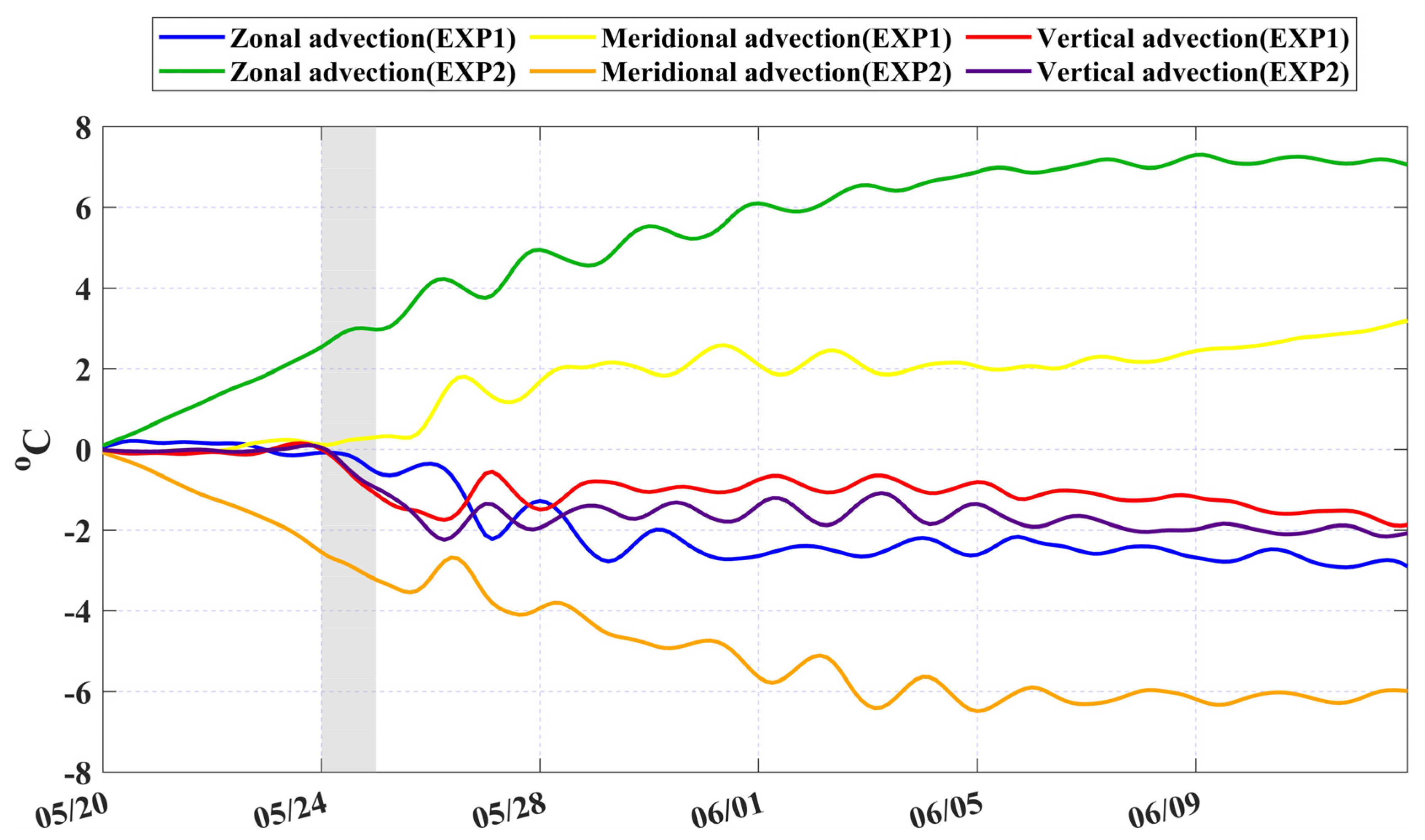
3.3.3. Heat Budget Analysis

To better identify the modulatory role of this cold eddy in the Mekunu-induced ocean temperature response, a heat budget analysis of the ocean above 200 m within region C in EXP1 and EXP2 was conducted using Equation (3). As evident from Figure 15, EXP1 and EXP2 yielded similar heat budget analysis results. During TC Mekunu’s passage, the vertical diffusion process primarily dominated the temperature change within the mixed layer, and the total advection process (horizontal advection + vertical advection) primarily dominated the subsurface temperature change. After TC Mekunu passed, the subsurface temperature exhibited an alternation of warming and cooling with a cycle of approximately 2 days dominated by the total advection process. This was closely related to the TC Mekunu-induced near-inertial oscillation in the upper ocean. These results are consistent with the findings proposed by Wu et al. [49].
The mixed-layer heat budgets within region C in EXP1 and EXP2 are given in Figure 16a,b. In EXP1 and EXP2, the maximum local rates of temperature change within the mixed layer were approximately −2.17 × 10⁻⁵ °C·s−1 and −1.65 × 10⁻⁵ °C·s−1, respectively, and the vertical diffusion terms at the corresponding moments were −2.00 × 10⁻⁵ °C·s−1 and −1.46 × 10⁻⁵ °C·s−1, respectively. This suggests that vertical diffusion accounted for 91.9% and 88.1% of the TC-induced MLT cooling trend in EXP1 and EXP2, respectively. Additionally, the cumulative contributions of vertical diffusion and total advection to MLT change were calculated (Figure 16c,d). In both EXP1 and EXP2, before the arrival of TC Mekunu (00:00 UTC on 20 May to 00:00 UTC on 23 May), the vertical diffusion process tended to slightly warm the mixed layer. As TC Mekunu gradually approached region C, the vertical diffusion process gradually enhanced MLT cooling under the combined effect of decreased shortwave radiation and increased latent heat loss at the sea surface and temperature stratification below the mixed layer, which contributed to approximately 2.89 °C cooling in EXP1 and 2.40 °C cooling in EXP2 at 00:00 UTC on 26 May. Given that the atmospheric forcing fields were the same in the two experiments, the greater MLT cooling in EXP1 was attributed to the steeper temperature stratification at the base of the mixed layer. Moreover, it is discernible that the contribution of vertical diffusion to MLT change before and after TC Mekunu’s passage exhibited an oscillating cycle of about 1 day because of the diurnal cycle of the heat flux. In contrast to that of vertical diffusion, the contribution of total advection was relatively low. During the passage of TC Mekunu, the cumulative contributions of the total advection process in EXP1 and EXP2 were only approximately −0.26 °C and −0.19 °C, respectively. One day after TC Mekunu’s passage, the total advection process gradually started to impede MLT cooling.
The subsurface temperature change was mainly attributed to the total advection process. The total advection term comprises zonal, meridional, and vertical advection components. Given that vertical diffusion tended to warm the water in the 50–100 m layer during TC Mekunu’s passage, we also calculated the cumulative contributions of these three advection terms to the temperature change in this layer (Figure 17). With TC Mekunu’s passage, zonal advection in EXP1 generally enhanced cooling in the 50–100 m layer, whereas meridional advection generally suppressed cooling. In EXP2, the contributions of zonal and meridional advection to the temperature change in the 50–100 m layer were exactly opposite those in EXP1. This suggests that the pre-existing cold eddy enhanced Mekunu-induced subsurface temperature cooling mainly through the zonal advection process, as reported in a previous study [63]. In both experiments, the contribution of vertical advection to temperature cooling was comparable during TC Mekunu’s passage. Nevertheless, during the relaxation stage, the cooling magnitude caused by vertical advection in EXP1 was smaller than that in EXP2, suggesting that the vertical advection process was not principally responsible for enhanced subsurface cooling under the presence of a pre-existing cold eddy. To put it more simply, this study revealed that horizontal advection could be modulated by a pre-existing cold eddy to enhance temperature cooling.

4. Conclusions

TC Mekunu was an ESCS system with an average translation speed of approximately 2.94 m·s−1. In this study, the atmospheric and oceanic states during TC Mekunu’s passage were reproduced by employing the COAWST model, and the simulation results were validated. Based on the simulated results and Argo observations, the upper ocean responses to TC Mekunu were examined. By using the stand-alone ROMS model, the role of a pre-existing cold eddy in modulating TC-induced temperature cooling was quantified.
Due to the Ekman pumping effect, significant changes in the oceanic mixed layer were induced by TC Mekunu. With TC Mekunu’s passage, the MLD on both sides of the track significantly deepened. Moreover, two cold patches (<26 °C) emerged to the right of TC Mekunu’s track, where the maximum MLT cooling reached 6.62 °C and 6.44 °C, respectively. The magnitude and the distribution of the MLD and MLT changes exhibited an obvious rightward bias on account of the resonance effect of the wind and near-inertial currents. Compared to the MLD and MLT changes, the MLS change was more complex. At the early stage of TC Mekunu’s development, the MLS on both sides of its track increased by approximately 0.5 psu. As TC Mekunu made landfall, the MLS differences in the coastal region were asymmetric, with the leftward MLS increasing and the rightward MLS decreasing by approximately 0.2 psu. It is noteworthy that a cold eddy pre-existed where the second cold patch emerged, and this eddy was intensified after TC Mekunu passed, with an average SSH reduction of approximately 2.7 cm.
In the subsurface, the Argo float 2901859 recorded a warming of approximately 1.9 °C at a depth of 100 m. Moreover, the COAWST simulations revealed that, in contrast to the rightward bias in MLT cooling, subsurface cooling within 150 km to the left of the TC Mekunu center was more significant, with a magnitude of approximately 5.5 °C. This was ascribed to the leftward movement of cold water on the right side of TC Mekunu’s track. Additionally, the magnitudes of temperature and salinity changes in the mixed and subsurface layers reached extreme values 1–2 days after TC Mekunu passed over the local ocean, indicating that the impacts of TC Mekunu on both the mixed and subsurface layers were delayed and persistent.
To assess the impact of the pre-existing cold eddy on the temperature response in the upper ocean, two model experiments were carried out by varying the ocean initial fields based on the stand-alone ocean model, corresponding to the cases of a pre-existing cold eddy and no eddy, respectively. Comparisons of the experimental results revealed that the cooling magnitude in the upper ocean was greater in the case that a cold eddy pre-existed along TC Mekunu’s track. Particularly, cooling within the mixed layer was enhanced by an average of approximately 0.41 °C owing to the steeper temperature stratification at the base of the mixed layer under the assumption of identical wind forcing. Moreover, heat budget analysis revealed that the vertical diffusion process dominated cooling in the mixed layer during the passage of TC Mekunu, while the subsurface temperature change was dominated by the total advection process. By calculating the cumulative contributions of zonal, meridional, and vertical advection terms to the temperature change in the 50–100 m layer, it was found that the zonal advection process mainly accounted for enhanced subsurface temperature cooling when a cold eddy pre-existed. In brief, our study revealed that horizontal advection could be modulated by a pre-existing cold eddy to enhance subsurface temperature cooling, which was underestimated in the previous studies.
In summary, the fully coupled atmosphere–ocean–wave model with high-temporal and -spatial resolutions could almost realistically reproduce the atmospheric and oceanic fields during the passage of TC Mekunu, and it may be useful in predicting extreme weather events over the region. Since the modulating effect of mesoscale cold eddies on the upper ocean responses to TCs has rarely been considered in the AS, although this is only a case study, the results demonstrate the contributions of various physical processes to the temperature response and highlight the importance of horizontal advection, which may contribute to explaining the air–sea interaction process when TCs encounter oceanic mesoscale eddies in the AS. Nevertheless, the simulated atmospheric and oceanic fields under TC conditions exhibited some bias, which might be limited by the initial and boundary conditions or the parameterization schemes, so their influence on model performance deserves further investigation. In addition, the effect of the horizontal advection process remains to be validated by observations. As reported by previous studies [36,42], parameters such as the TC intensity, TC translation speed, eddy strength, and position of the eddy relative to the TC affect upper ocean responses to TCs. In the future, the relative importance of these parameters to the modulated upper ocean responses by oceanic mesoscale eddies will be further investigated.

Author Contributions

Conceptualization and methodology, D.R. and S.W.; software and resources, S.H.; funding acquisition, S.H.; validation and formal analysis, D.R.; writing—original draft preparation, D.R.; writing—review and editing, S.H. and D.R. All authors have read and agreed to the published version of the manuscript.

Funding

This research was funded by the National Key Research and Development Program of China (No. 2022YFC3104000) and the Innovation Research Project for Marine Science and Technology of Jiangsu Province (No. JSZRHYKJ202304).

Institutional Review Board Statement

Not applicable.

Informed Consent Statement

Not applicable.

Data Availability Statement

The data presented in this study are available on reasonable request from the corresponding author.

Acknowledgments

We are very thankful to the Indian Meteorological Department for providing tropical cyclone information, the China Argo Real-time Data Center for providing Argo profiles, the National Centers for Environmental Prediction for providing the atmospheric data and the Hybrid Coordinate Ocean Model for providing the oceanic fields data.

Conflicts of Interest

The authors declare no conflicts of interest.

References

  1. Sahoo, B.; Bhaskaran, P.K. Assessment on historical cyclone tracks in the Bay of Bengal, east coast of India. Int. J. Climatol. 2016, 36, 95–109. [Google Scholar] [CrossRef]
  2. Singh, V.K.; Roxy, M.K. A review of ocean-atmosphere interactions during tropical cyclones in the north Indian Ocean. Earth-Sci. Rev. 2022, 226, 103967. [Google Scholar] [CrossRef]
  3. Kumar, S.P.; Roshin, R.P.; Narvekar, J.; Kumar, P.K.D.; Vivekanandan, E. Response of the Arabian Sea to global warming and associated regional climate shift. Mar. Environ. Res. 2009, 68, 217–222. [Google Scholar] [CrossRef] [PubMed]
  4. Murakami, H.; Vecchi, G.A.; Underwood, S. Increasing frequency of extremely severe cyclonic storms over the Arabian Sea. Nat. Clim. Chang. 2017, 7, 885–889. [Google Scholar] [CrossRef]
  5. Bell, S.S.; Chand, S.S.; Tory, K.J.; Ye, H.; Turville, C. North Indian Ocean tropical cyclone activity in CMIP5 experiments: Future projections using a model-independent detection and tracking scheme. Int. J. Climatol. 2020, 40, 6492–6505. [Google Scholar] [CrossRef]
  6. Price, J.F.; Sanford, T.B.; Forristall, G.Z. Forced Stage Response to a Moving Hurricane. Am. Meteorol. Soc. 1994, 24, 233–260. [Google Scholar] [CrossRef]
  7. Yang, B.; Hou, Y. Near-inertial waves in the wake of 2011 Typhoon Nesat in the northern South China Sea. Acta Oceanol. Sin. 2014, 33, 102–111. [Google Scholar] [CrossRef]
  8. Chen, G.; Xue, H.; Wang, D.; Xie, Q. Observed near-inertial kinetic energy in the northwestern South China Sea. J. Geophys. Res. Oceans 2013, 118, 4965–4977. [Google Scholar] [CrossRef]
  9. Kawaguchi, Y.; Yabe, I.; Senjyu, T.; Sakai, A. Amplification of typhoon-generated near-inertial internal waves observed near the Tsushima oceanic front in the Sea of Japan. Sci. Rep. 2023, 13, 8387. [Google Scholar] [CrossRef]
  10. Price, J.F. Upper Ocean Response to a Hurricane. J. Phys. Oceanogr. 1981, 11, 153–175. [Google Scholar] [CrossRef]
  11. Mei, W.; Pasquero, C. Spatial and Temporal Characterization of Sea Surface Temperature Response to Tropical Cyclones. J. Clim. 2013, 26, 3745–3765. [Google Scholar] [CrossRef]
  12. D’Asaro, E.A.; Sanford, T.B.; Niiler, P.P.; Terrill, E.J. Cold wake of Hurricane Frances. Geophys. Res. Lett. 2007, 34. [Google Scholar] [CrossRef]
  13. Mahapatra, D.K.; Rao, A.D.; Babu, S.V.; Srinivas, C. Influence of coast line on upper ocean’s response to the tropical cyclone. Geophys. Res. Lett. 2007, 34, L17603. [Google Scholar] [CrossRef]
  14. Huang, P.; Sanford, T.B.; Imberger, J. Heat and turbulent kinetic energy budgets for surface layer cooling induced by the passage of Hurricane Frances (2004). J. Geophys. Res. Oceans 2009, 114, 1–14. [Google Scholar] [CrossRef]
  15. Vincent, E.M.; Lengaigne, M.; Madec, G.; Vialard, J.; Samson, G.; Jourdain, N.C.; Menkes, C.E.; Jullien, S. Processes setting the characteristics of sea surface cooling induced by tropical cyclones. J. Geophys. Res. Oceans 2012, 117. [Google Scholar] [CrossRef]
  16. Zedler, S.E.; Dickey, T.D.; Doney, S.C.; Price, J.F.; Yu, X.; Mellor, G.L. Analyses and simulations of the upper ocean’s response to Hurricane Felix at the Bermuda Testbed Mooring site: 13–23 August 1995. J. Geophys. Res. Oceans 2002, 107, 25-1–25-29. [Google Scholar] [CrossRef]
  17. Emanuel, K. Contribution of tropical cyclones to meridional heat transport by the oceans. J. Geophys. Res. Atmos. 2001, 106, 14771–14781. [Google Scholar] [CrossRef]
  18. Sriver, R.L.; Huber, M. Observational evidence for an ocean heat pump induced by tropical cyclones. Nature 2007, 447, 577–580. [Google Scholar] [CrossRef] [PubMed]
  19. Pasquero, C.; Emanuel, K. Tropical Cyclones and Transient Upper-Ocean Warming. J. Clim. 2008, 21, 149–162. [Google Scholar] [CrossRef]
  20. Hart, R.E.; Maue, R.N.; Watson, M.C. Estimating Local Memory of Tropical Cyclones through MPI Anomaly Evolution. Mon. Weather Rev. 2007, 135, 3990–4005. [Google Scholar] [CrossRef]
  21. Park, J.J.; Kwon, Y.; Price, J.F. Argo array observation of ocean heat content changes induced by tropical cyclones in the north Pacific. J. Geophys. Res. Oceans 2011, 116. [Google Scholar] [CrossRef]
  22. Robertson, E.J.; Ginis, I. The Upper Ocean Salinity Response to Tropical Cyclones. Preprints. In Proceedings of the 25th Conference on Hurricanes and Tropical Meteorology, San Diego, CA, USA, 29 April–3 May 2002; American Meteorological Society: Boston, MA, USA, 2002. [Google Scholar]
  23. Girishkumar, M.S.; Suprit, K.; Chiranjivi, J.; Bhaskar, T.V.S.U.; Ravichandran, M.; Shesu, R.V.; Rao, E.P.R. Observed oceanic response to tropical cyclone Jal from a moored buoy in the south-western Bay of Bengal. Ocean Dyn. 2014, 64, 325–335. [Google Scholar] [CrossRef]
  24. Chaudhuri, D.; Sengupta, D.; Asaro, E.D.; Venkatesan, R.; Ravichandran, M. Response of the Salinity-Stratified Bay of Bengal to Cyclone Phailin. J. Phys. Oceanogr. 2019, 49, 1121–1140. [Google Scholar] [CrossRef]
  25. Qiu, Y.; Han, W.; Lin, X.; West, B.J.; Li, Y.; Xing, W.; Zhang, X.; Arulananthan, K.; Guo, X. Upper-Ocean Response to the Super Tropical Cyclone Phailin (2013) over the Freshwater Region of the Bay of Bengal. J. Phys. Oceanogr. 2019, 49, 1201–1228. [Google Scholar] [CrossRef]
  26. Chacko, N. Insights into the haline variability induced by cyclone Vardah in the Bay of Bengal using SMAP salinity observations. Remote Sens. Lett. 2018, 9, 1205–1213. [Google Scholar] [CrossRef]
  27. Mei, W.; Pasquero, C.; Primeau, F. The effect of translation speed upon the intensity of tropical cyclones over the tropical ocean. Geophys. Res. Lett. 2012, 39. [Google Scholar] [CrossRef]
  28. Dare, R.A.; McBride, J.L. Sea Surface Temperature Response to Tropical Cyclones. Mon. Weather Rev. 2011, 139, 3798–3808. [Google Scholar] [CrossRef]
  29. Behera, S.K.; Deo, A.A.; Salvekar, P.S. Investigation of mixed layer response to Bay of Bengal cyclone using a simple ocean model. Meteorog. Atmos. Phys. 1998, 65, 77–91. [Google Scholar] [CrossRef]
  30. Liu, Y.; Guan, S.; Lin, I.I.; Mei, W.; Jin, F.; Huang, M.; Zhang, Y.; Zhao, W.; Tian, J. Effect of Storm Size on Sea Surface Cooling and Tropical Cyclone Intensification in the Western North Pacific. J. Clim. 2023, 36, 7277–7296. [Google Scholar] [CrossRef]
  31. Elizabeth, A.I.; Effy, J.B.; Francis, P.A. On the upper ocean response of Bay of Bengal to very severe cyclones Phailin and Hudhud. J. Oper. Oceanogr. 2022, 15, 17–31. [Google Scholar] [CrossRef]
  32. Lin, S.; Zhang, W.; Shang, S.; Hong, H. Ocean response to typhoons in the western North Pacific: Composite results from Argo data. Deep. Sea Res. Part. I Oceanogr. Res. Pap. 2017, 123, 62–74. [Google Scholar] [CrossRef]
  33. Sun, J.; Vecchi, G.; Sodn, B. Sea Surface Salinity Response to Tropical Cyclones Based on Satellite Observations. Remote Sens. 2021, 13, 420. [Google Scholar] [CrossRef]
  34. Shay, L.K.; Goni, G.J.; Black, P.G. Effects of a Warm Oceanic Feature on Hurricane Opal. Mon. Weather Rev. 2000, 128, 1366–1383. [Google Scholar] [CrossRef]
  35. Jaimes, B.; Shay, L.K. Mixed Layer Cooling in Mesoscale Oceanic Eddies during Hurricanes Katrina and Rita. Mon. Weather Rev. 2009, 137, 4188–4207. [Google Scholar] [CrossRef]
  36. Ma, Z.; Fei, J.; Liu, L.; Huang, X.; Li, Y. An Investigation of the Influences of Mesoscale Ocean Eddies on Tropical Cyclone Intensities. Mon. Weather Rev. 2017, 145, 1181–1201. [Google Scholar] [CrossRef]
  37. Jacob, S.D.; Shay, L.K. The Role of Oceanic Mesoscale Features on the Tropical Cyclone–Induced Mixed Layer Response: A Case Study. J. Phys. Oceanogr. 2003, 33, 649–676. [Google Scholar] [CrossRef]
  38. Lu, Z.; Wang, G.; Shang, X. Response of a Preexisting Cyclonic Ocean Eddy to a Typhoon. J. Phys. Oceanogr. 2016, 46, 2403–2410. [Google Scholar] [CrossRef]
  39. Gordon, A.L.; Shroyer, E.; Murty, V.S.N. An Intrathermocline Eddy and a tropical cyclone in the Bay of Bengal. Sci. Rep. 2017, 7, 46218. [Google Scholar] [CrossRef]
  40. Sun, L.; Li, Y.X.; Yang, Y.J.; Wu, Q.; Chen, X.T.; Li, Q.Y.; Li, Y.B.; Xian, T. Effects of super typhoons on cyclonic ocean eddies in the western North Pacific: A satellite data-based evaluation between 2000 and 2008. J. Geophys. Res. Oceans 2014, 119, 5585–5598. [Google Scholar] [CrossRef]
  41. Zheng, Z.W.; Ho, C.R.; Kuo, N.J. Importance of pre-existing oceanic conditions to upper ocean response induced by Super Typhoon Hai-Tang. Geophys. Res. Lett. 2008, 35, L20603. [Google Scholar] [CrossRef]
  42. Yablonsky, R.M.; Ginis, I. Impact of a Warm Ocean Eddy’s Circulation on Hurricane-Induced Sea Surface Cooling with Implications for Hurricane Intensity. Mon. Weather Rev. 2012, 141, 997–1021. [Google Scholar] [CrossRef]
  43. Guan, S.; Liu, Z.; Song, J.; Hou, Y.; Feng, L. Upper ocean response to Super Typhoon Tembin (2012) explored using multiplatform satellites and Argo float observations. Int. J. Remote Sens. 2017, 38, 5150–5167. [Google Scholar] [CrossRef]
  44. Prakash, K.R.; Nigam, T.; Pant, V.; Chandra, N. On the interaction of mesoscale eddies and a tropical cyclone in the Bay of Bengal. Nat. Hazards 2021, 106, 1981–2001. [Google Scholar] [CrossRef]
  45. Warner, J.C.; Armstrong, B.; He, R.; Zambon, J.B. Development of a Coupled Ocean-Atmosphere-Wave-Sediment Transport (COAWST) Modeling System. Ocean Model. 2010, 35, 230–244. [Google Scholar] [CrossRef]
  46. Larson, J.; Jacob, R.; Ong, E. The Model Coupling Toolkit: A New Fortran90 Toolkit for Building Multiphysics Parallel Coupled Models. Int. J. High Perform. Comput. Appl. 2005, 19, 277–292. [Google Scholar] [CrossRef]
  47. Lim Kam Sian, K.T.C.; Dong, C.; Liu, H.; Wu, R.; Zhang, H. Effects of Model Coupling on Typhoon Kalmaegi (2014) Simulation in the South China Sea. Atmosphere 2020, 11, 432. [Google Scholar] [CrossRef]
  48. Zambon, J.B.; He, R.; Warner, J.C. Investigation of hurricane Ivan using the coupled ocean-atmosphere-wave-sediment transport (COAWST) model. Ocean Dyn. 2014, 64, 1535–1554. [Google Scholar] [CrossRef]
  49. Wu, R.; Zhang, H.; Chen, D.; Li, C.; Lin, J. Impact of Typhoon Kalmaegi (2014) on the South China Sea: Simulations using a fully coupled atmosphere-ocean-wave model. Ocean Model. 2018, 131, 132–151. [Google Scholar] [CrossRef]
  50. Warner, J.C.; Sherwood, C.R.; Arango, H.G.; Signell, R.P. Performance of four turbulence closure models implemented using a generic length scale method. Ocean Model. 2005, 8, 81–113. [Google Scholar] [CrossRef]
  51. de Boyer Montégut, C.; Madec, G.; Fischer, A.S.; Lazar, A.; Iudicone, D. Mixed layer depth over the global ocean: An examination of profile data and a profile-based climatology. J. Geophys. Res. Oceans 2004, 109. [Google Scholar] [CrossRef]
  52. Liu, N.; Ling, T.; Wang, H.; Zhang, Y.; Gao, Z.; Wang, Y. Numerical simulation of Typhoon Muifa (2011) using a Coupled Ocean-Atmosphere-Wave-Sediment Transport (COAWST) modeling system. J. Ocean Univ. 2015, 14, 199–209. [Google Scholar] [CrossRef]
  53. Thompson, B.; Sanchez, C.; Sun, X.; Song, G.; Liu, J.; Huang, X.; Tkalich, P. A high-resolution atmosphere–ocean coupled model for the western Maritime Continent: Development and preliminary assessment. Clim. Dyn. 2019, 52, 3951–3981. [Google Scholar] [CrossRef]
  54. Yang, Z.; Richardson, P.; Chen, Y.; Kelley, J.G.W.; Myers, E.; Aikman, F.; Peng, M.; Zhang, A. Model Development and Hindcast Simulations of NOAA’s Gulf of Maine Operational Forecast System. J. Mar. Sci. Eng. 2016, 4, 77. [Google Scholar] [CrossRef]
  55. Krishna, K.M. Observational study of upper ocean cooling due to Phet super cyclone in the Arabian Sea. Adv. Space Res. 2016, 57, 2115–2120. [Google Scholar] [CrossRef]
  56. Roy Chowdhury, R.; Prasanna Kumar, S.; Narvekar, J.; Chakraborty, A. Back-to-Back Occurrence of Tropical Cyclones in the Arabian Sea During October-November 2015: Causes and Responses. J. Geophys. Res. Oceans 2020, 125, e2019JC015836. [Google Scholar] [CrossRef]
  57. Price, J.F.; Weller, R.A.; Pinkel, R. Diurnal cycling: Observations and models of the upper ocean response to diurnal heating, cooling, and wind mixing. J. Geophys. Res. Oceans 1986, 91, 8411–8427. [Google Scholar] [CrossRef]
  58. Price, J.F. Internal Wave Wake of a Moving Storm. Part I. Scales, Energy Budget and Observations. J. Phys. Oceanogr. 1983, 13, 949–965. [Google Scholar] [CrossRef]
  59. Kwon, Y.O. Observation of General Circulation and Water Mass Variability in the North Atlantic Subtropical Mode Water Region. Ph.D. Thesis, University of Washington: Seattle, WA, USA, 2003. [Google Scholar]
  60. Baranowski, D.B.; Flatau, P.J.; Chen, S.; Black, P.G. Upper ocean response to the passage of two sequential typhoons. Ocean Sci. 2014, 10, 559–570. [Google Scholar] [CrossRef]
  61. Liu, S.; Sun, L.; Wu, Q.; Yang, Y. The responses of cyclonic and anticyclonic eddies to typhoon forcing: The vertical temperature-salinity structure changes associated with the horizontal convergence/divergence. J. Geophys. Res. Oceans 2017, 122, 4974–4989. [Google Scholar] [CrossRef]
  62. Lin, I.; Wu, C.; Emanuel, K.A.; Lee, I.; Wu, C.; Pun, I. The Interaction of Supertyphoon Maemi (2003) with a Warm Ocean Eddy. Mon. Weather Rev. 2005, 133, 2635–2649. [Google Scholar] [CrossRef]
  63. Li, X.; Cheng, X.; Fei, J.; Huang, X. A Numerical Study on the Role of Mesoscale Cold-Core Eddies in Modulating the Upper-Ocean Responses to Typhoon Trami (2018). J. Phys. Oceanogr. 2022, 52, 3101–3122. [Google Scholar] [CrossRef]
  64. Yu, J.; Lin, S.; Jiang, Y.; Wang, Y. Modulation of Typhoon-Induced Sea Surface Cooling by Preexisting Eddies in the South China Sea. Water 2021, 13, 653. [Google Scholar] [CrossRef]
Figure 1. Model domains for the WRF (black box) and ROMS (red box) models in the AS. The shading denotes the bathymetry.
Jmse 12 01177 g001
Figure 2. (a) COAWST model-simulated track (black dashed line) and IMD best track (black solid line) for TC Mekunu. The dots denote the positions of TC Mekunu center and their colors denote the intensity of TC Mekunu. The black pentagrams denote the positions of the Argo float (number 2901859) before and after the passage of TC Mekunu. The red solid line denotes the position of the S1 transect. This Argo float and S1 transect were used to analyze the subsurface response in Section 3.2.3. (b) Errors of the simulated locations of TC Mekunu center. The x-axis labels indicate the time in month/day/hour format (MM/DD/HH in UTC).
Jmse 12 01177 g002
Figure 3. Comparisons of the COAWST simulated (a) central air pressure and (b) maximum wind speed of TC Mekunu against those provided by the IMD and FNL data. The x-axis labels indicate the time in month/day/hour format (MM/DD/HH in UTC).
Jmse 12 01177 g003
Figure 4. Comparisons of the (a) temperature and (b) salinity between the COAWST simulations and Argo observations. The red solid lines denote the linear fit curves. The solid green lines denote the 95% confidence intervals.
Jmse 12 01177 g004
Figure 5. (af) Evolution of the sea surface height (SSH, shading) and sea surface currents (black arrows) before, during, and after TC Mekunu’s passage. The simulated track of TC Mekunu (black dashed lines) is overlaid, with the position and intensity depicted by colored dots. The black box in (a) marks the pre-existing cold eddy.
Jmse 12 01177 g005
Figure 6. (af) Evolution of the Ekman pumping velocity (EPV, shading) before, during, and after TC Mekunu’s passage. The black arrows indicate the 10 m wind vectors. The simulated track of TC Mekunu (black dashed lines) is overlaid, with the position and intensity depicted by colored dots.
Jmse 12 01177 g006
Figure 7. (ah) Evolution of the mixed layer depth (MLD) before, during, and after TC Mekunu’s passage. (i) MLD differences at 00:00 UTC on 26 May with respect to the mean MLD on 20 May. The black solid lines denote the MLD contours. The simulated track of TC Mekunu (black dashed lines) is overlaid, with the position and intensity depicted by colored dots.
Jmse 12 01177 g007
Figure 8. (ah) Evolution of the mixed layer temperature (MLT) before, during, and after TC Mekunu’s passage. (i) MLT differences at 00:00 UTC on 26 May with respect to the mean MLT on 20 May. The black solid lines denote the MLT contours. The simulated track of TC Mekunu (black dashed lines) is overlaid, with the position and intensity depicted by colored dots.
Jmse 12 01177 g008
Figure 9. (ah) Evolution of the mixed layer salinity (MLS) before, during, and after TC Mekunu’s passage. (i) MLS differences at 00:00 UTC on 26 May with respect to the mean MLS on 20 May. The black solid lines denote the MLS contours. The simulated track of TC Mekunu (black dashed lines) is overlaid, with the position and intensity depicted by colored dots.
Jmse 12 01177 g009
Figure 10. Profiles of the (a) temperature, (b) salinity, and (c) density before (i.e., pre-Mekunu) and after (i.e., post-Mekunu) TC Mekunu’s passage. Changes in the (d) temperature, (e) salinity, and (f) density based on the Argo observations.
Jmse 12 01177 g010
Figure 11. Evolution of the temperature (shading) above 200 m along the transect (i.e., the red line in Figure 2a) before, during, and after TC Mekunu’s passage. The black solid lines indicate the temperature contours. The green solid lines denote the MLD along the transect. The black dashed lines denote the longitudinal position of the TC Mekunu center at 06:00 UTC on 24 May.
Jmse 12 01177 g011
Figure 12. Distribution of the SSH, MLD, and D26 on 20 May in (ac) EXP1 and (df) EXP2. The track of TC Mekunu derived from the IMD (black dashed lines) is overlaid. The black boxes mark region C, which encompasses a pre-existing cold eddy.
Jmse 12 01177 g012
Figure 13. (a,b) MLD differences and (c,d) MLT differences at 00:00 UTC on 26 May with respect to the mean MLD/MLT on 20 May. The black solid lines denote the contours of the MLD/MLT differences. The track of TC Mekunu derived from the IMD (black dashed lines) is overlaid, with the position and intensity depicted by colored dots.
Jmse 12 01177 g013
Figure 14. (a) Temperature profiles on 20 May (i.e., pre-Mekunu) and at the time of maximum MLT cooling after TC Mekunu’s passage (i.e., post-Mekunu) at P1 in EXP1 and EXP2. (b) Temperature changes at P1 in EXP1 and EXP2.
Jmse 12 01177 g014
Figure 15. Heat budget analysis of the ocean above 200 m within region C in EXP1 and EXP2: (a,b) Local rate of temperature change, (c,d) vertical diffusion term, (e,f) total advection term (horizontal advection + vertical advection). The green solid lines denote the mean MLD in region C. The black dashed lines denote the moments when TC Mekunu entered and left region C. The x-axis labels indicate the time in month/day format (MM/DD in UTC).
Jmse 12 01177 g015
Figure 16. Mixed-layer heat budget analysis within region C in (a) EXP1 and (b) EXP2. Cumulative contributions of (c) vertical diffusion and (d) total advection to MLT change. The gray shading indicates the moment when the TC Mekunu center passed over region C. The x-axis labels indicate the time in month/day format (MM/DD in UTC).
Jmse 12 01177 g016
Figure 17. Cumulative contributions of zonal, meridional, and vertical advection to the temperature change in the 50–100 m layer. The gray shading indicates the moment when the TC Mekunu center passed over region C. The x-axis labels indicate the time in month/day format (MM/DD in UTC).
Jmse 12 01177 g017
Table 1. Parameter settings of the WRF model.
ParameterScheme
Near surface layerMonin–Obukhov
Land surfaceNoah
Planetary boundary layerYSU
Longwave radiationRRTM
Shortwave radiationDudhia
MicrophysicsWSM3
Cumulus convectionKain–Fritsch
Table 2. Characteristics of the mixed layer observed by the Argo float.
DateMLD (m)MLT (°C)MLS (psu)
21 May 201821.230.036.2
31 May 201830.028.036.3
Table 3. Ocean conditions averaged within region C on 20 May in the two experiments.
ExperimentSSH (m)MLD (m)D26 (m)
EXP10.3117.0451.26
EXP20.3618.1656.34
Disclaimer/Publisher’s Note: The statements, opinions and data contained in all publications are solely those of the individual author(s) and contributor(s) and not of MDPI and/or the editor(s). MDPI and/or the editor(s) disclaim responsibility for any injury to people or property resulting from any ideas, methods, instructions or products referred to in the content.

