Unveiling Turbulent Flow Dynamics in Blind-Tee Pipelines: Enhancing Fluid Mixing in Subsea Pipeline Systems

Abstract

Blind tees, as important junctions, are widely used in offshore oil and gas transportation systems to improve mixing flow conditions and measurement accuracies in curved pipes. Despite the significance of blind tees, their unsteady flow characteristics and mixing mechanisms in turbulent flow regimes are not clearly established. Therefore, in this study, Unsteady Reynolds-Averaged Navier–Stokes (URANS) simulations, coupled with Explicit Algebraic Reynolds Stress Model (EARSM), are employed to explore the complex turbulent flow characteristics within blind-tee pipes. Firstly, the statistical flow features are investigated based on the time-averaged results, and the swirl dissipation analysis reveals an intense dissipative process occurring within blind tees, surpassing conventional elbows in swirling intensity. Then, the instantaneous flow characteristics are investigated through time and frequency domain analysis, uncovering the oscillatory patterns and elucidating the mechanisms behind unsteady secondary flow motions. In a 2D-length blind tee, a nondimensional dominant frequency of oscillation (St_bt = 0.0361) is identified, highlighting the significant correlation between dominant frequencies inside and downstream of the plugged section, which emphasizes the critical role of the plugged structure in these unsteady motions. Finally, a power spectra analysis is conducted to explore the influence of blind-tee structures, indicating that the blind-tee length of l_bt = 2D enhances the flow-mixing conditions by amplifying the oscillation intensities of secondary flow motions.

1. Introduction

Blind tees, pivotal components in fluid transportation systems, hold immense importance in optimizing the mixing conditions essential for flow control and measurements within curved structures, particularly in subsea oil and gas pipelines. The complexities stemming from the turbulent flow characteristics of these blind-tee pipes constitute a crucial aspect in elucidating fluid mixing mechanisms. In the domain of ocean engineering, pipelines demand meticulous design considerations, and are often configured as multi-bending structures and interconnected by various junctions such as bends, T-junctions, and blind tees [1,2]. Notably, the flow dynamics near these junctions markedly differ from those in straight pipes owing to directional changes, underscoring the necessity for comprehensive investigation.

Within the bending structure of subsea oil and gas transportation pipelines, the secondary flow arises from the curvature, overlaying with the primary flow due to centrifugal force. This leads to swift fluid redirection towards the inner-side corner along the pipe wall, while slower-moving fluid is directed towards the outer-side corner along the pipe’s centerline. Dean et al. [3] investigated this phenomenon analytically in a curved channel and proposed an important governing parameter, i.e., the Dean number $De=\mathrm{Re}\sqrt{D/2R_c}$, where D is the pipe diameter, Re is the Reynolds number, and R_c is the radius of the bend curvature. Since then, the flow through the curved channel has gained widespread attention since it is related to nearly all the equipment used in the industrial process. Early-stage studies have focused on the laminar flow regime. Winters [4] studied the bifurcation of the laminar flow in the bent channel’s square section, and pointed out the critical symmetry-breaking aspect ratio. Bara et al. [5] employed Laser–Doppler measurements to study the vortex evolution in the square curved channel and indicated the critical De number characterizing the bifurcation of vortices. In terms of the bends in the circular cross section, some researchers analytically and numerically studied the evolution behavior of the counter-rotating vortices, also known as Dean vortices, from single-pair to multi-pair in laminar flow regimes [6,7,8].

In recent decades, ocean engineering has witnessed extensive research into turbulent flow within curved pipes and the intricate design of complex pipeline configurations [9,10]. Sudo et al. [11,12] conducted detailed investigations into the statistical properties of turbulent flow in curved pipes with circular and square sections, and utilized hot-wire measurements to establish how the bend curvatures influence the strength of secondary flow. Jurga et al. [13] explored the impact of Reynolds number and curvature ratio on velocity distributions and pressure gradients in turbulent bent flows. Han et al. [14] thoroughly investigated secondary flow characteristics in double-curved pipes, providing comprehensive insights into the structural influences of continuous bends. Additionally, studies were conducted on the turbulent flow characteristics inside special bending structures, including T-junctions and blind tees. Kumar et al. [15] analyzed the flow separations inside a T-shaped structure at Re = 5300 using direct numerical simulations. Zhang et al. [16] analyzed the flow-induced noise characteristics in a closed-branch T-junction at Re = 20,000 using dynamic delayed detached-eddy simulations. Lan et al. [17] investigated the turbulent flow in a blind-tee pipe at different Reynolds numbers (Re = 5000, 20,000 and 40,000). The results show that with the increase in Reynolds number, the primary vortex size increases, the secondary vortex size decreases, and the region of low-speed flow circulation in the blind end increases.

Furthermore, the study of unsteady flow characteristics in bent pipes has received significant attention. Tunstall and Harvey [18] undertook pioneering work on the unsteady turbulent features in bends, analyzed the dynamics of Dean vortices, revealed the frequency characteristics, and explained their origins. However, technological limitations have prevented in-depth investigations on the unsteady behaviors of turbulent flow in bends for decades until recent advancements in experimental and computational techniques. Hellström et al. [19] indicated that the fluid motion in a 90° bend produced single-vortex structures in both clockwise and anti-clockwise rotations, which deviated from the known Dean vortices. They highlighted two dominant Strouhal numbers for the swirl switches in order to characterize the unsteady fluid motion. Sarkodie et al. [20] and Liu et al. [21] demonstrated unsteady vortex structures using non-intrusive optical sensors and particle image velocimetry (PIV) experiments. Employing direct numerical simulation (DNS), Hufnagel et al. [22] identified the swirl switch mechanism as a wave-like structure originating from curvature. Luo et al. [23] delved into the near-wall shear stress using Large Eddy Simulation (LES) and pointed out that the swirl switch is a primary factor contributing to bend fatigue in oil and gas transportation.

In addressing multiphase flow characteristics and fluid–structure interactions prevalent in offshore oil and gas transportation processes, De Rosis and Tafuni [24] analyzed the water-entry and water-exit phenomena using the lattice Boltzmann method (LBM) and smooth particle hydrodynamics simulations (SPH). Li et al. [25] utilized electrical capacitance tomography (ECT) and convolutional neural network (CNN) techniques to experimentally identify multiphase flow patterns within pipeline systems, achieving an impressive accuracy rate of 97.55%.

Additionally, studies have explored flow behaviors within various junctions integral to ocean engineering, such as T-junctions [26], Y-junctions [27], and blind tees [28]. Among them, the T- and Y-junctions are structures with one inlet and two outlets (or two inlets and one outlet). These are commonly used for flow diversion, merging, etc. Different from a T-junction, a blind tee is a special bending structure with one inlet, one outlet, and a branch that is sealed off (i.e., the blind end). It is designed to enhance fluid mixing conditions for precise flow measurements, and the backflow formed within the blind end aids in mixing the main flow downstream of the bend. This is widely utilized in subsea production systems [29,30]. Previous investigations have examined the flow mechanisms within blind-tee pipes under laminar flow conditions. Han et al. [31,32] delved into the flow-mixing mechanisms within blind-tee pipes and analyzed the structural influences of the blind end. Moreover, Liu et al. [33] explored the impacts of blind tees and structural parameters on flow-mixing patterns in pipelines with multiple bends.

Despite the importance of blind tees in the industrial applications of subsea oil and gas pipelines, research on turbulent flow characteristics in pipelines with blind tees remains limited, and previous investigations [17,34] mainly focused on the steady-state features of turbulent flow in blind tees. However, few studies have been conducted on the unsteady characteristics of turbulent flow in blind-tee pipes. Moreover, as a commonly used flow-mixing device in the offshore oil and gas industry, the mechanism of how the blind tee enhances the flow mixing in bend pipes has still not been clearly revealed, especially the time–frequency relationship between the flow circulation inside the blind end and the secondary flow downstream of the bend, which significantly affects the reliability and safety of bending structures in offshore pipeline systems. Therefore, considering the turbulence anisotropy, this study employs the Explicit Algebraic Reynolds Stress Model (EARSM) to further explore the unsteady characteristics of turbulent flow in blind-tee pipes. To this end, qualitative and quantitative insights are provided into the time-averaged flow features in a blind-tee pipe at first. Then, the oscillatory flow patterns inside and downstream of the plugged section are captured by taking instantaneous snapshots of the flow field, and corresponding velocity frequency spectra in the blind tee are systematically analyzed. Ultimately, the structural influences are evaluated to achieve an optimal blind-tee structure via comparisons in both time and frequency domains, with the expectation of developing an in-depth understanding of their mixing mechanisms and providing references for the optimization of the design of blind-tee pipes in offshore industrial applications.

2. Numerical Methods

2.1. Governing Equations

This study employs Unsteady Reynolds-Averaged Navier–Stokes (URANS) equations of continuity and momentum to model the incompressible flow within the blind-tee pipes.

$${\displaystyle \frac{\partial u_i}{\partial x_i}}=0$$

(1)

$${\displaystyle \frac{\partial u_i}{\partial t}}+u_j{\displaystyle \frac{\partial u_i}{\partial x_j}}=-{\displaystyle \frac{1}{\rho }}{\displaystyle \frac{\partial p}{\partial x_i}}+{\displaystyle \frac{\partial }{\partial x_j}}\left(\nu {\displaystyle \frac{\partial u_i}{\partial x_j}}-\overline{u_i^{\prime }{u}_j^{\prime }}\right)$$

(2)

where $x_i$ and $x_j$ denote the Cartesian coordinates in three directions (i, j = 1, 2 and 3), and the symbols $u_i$, $u_j$, $p$, $\rho$, and $\nu$ are the corresponding Reynolds-averaged velocities, dynamic pressure, density, and kinematic viscosity of the fluid, respectively. $\overline{u_i^{\prime }{u}_j^{\prime }}$ is the Reynolds stress tensor consisting of the fluctuating part of the velocity.

In this paper, the EARSM model is adopted to solve turbulent flow issues in blind-tee pipes. It relates the Reynolds stress with the mean strain rate and vorticity tensors [35], which avoids using the Boussinesq assumption [36,37]. Accordingly, the Reynold stress tensor term is given as follows:

$$\overline{u_i^{\prime }{u}_j^{\prime }}=k\left(a_{ij}+\frac{2}{3}{\delta }_{ij}\right)$$

(3)

$$\begin{array}{l}{a}_{ij}={\beta }_1{S}_{ij}+{\beta }_3({\mathrm{\Omega }}_{ik}{\mathrm{\Omega }}_{kj}-\frac{1}{3}{\mathrm{\Omega }}_{kl}{\mathrm{\Omega }}_{lk}{\delta }_{ij})+{\beta }_4(S_{ik}{\mathrm{\Omega }}_{kj}-{\mathrm{\Omega }}_{ik}{S}_{kj})\\ +{\beta }_6(S_{ik}{\mathrm{\Omega }}_{kl}{\mathrm{\Omega }}_{lj}+{\mathrm{\Omega }}_{ik}{\mathrm{\Omega }}_{kl}{S}_{lj}-{\displaystyle \frac{2}{3}}{S}_{kl}{\mathrm{\Omega }}_{lm}{\mathrm{\Omega }}_{mk}{\delta }_{ij}-{\mathrm{\Omega }}_{kl}{\mathrm{\Omega }}_{lk}{S}_{ij})\end{array}$$

(4)

$$S_{ij}={\displaystyle \frac{1}{2}}\tau ({\displaystyle \frac{\partial u_i}{\partial x_j}}+{\displaystyle \frac{\partial u_j}{\partial x_i}})$$

(5)

$${\mathrm{\Omega }}_{ij}={\displaystyle \frac{1}{2}}\tau ({\displaystyle \frac{\partial u_i}{\partial x_j}}-{\displaystyle \frac{\partial u_j}{\partial x_i}})$$

(6)

$$\tau =1/(C_{\mu }\omega )$$

(7)

where k is the turbulence kinetic energy, the indices i, j, k, l and m = 1, 2 and 3 represent different Cartesian coordinates, ${\delta }_{ij}$ is the Kronecker delta, $a_{ij}$ represents the anisotropy tensor, ${\beta }_i$ represents the coefficient of the tensor basis, $\omega$ is the turbulence dissipation rate, and $C_{\mu }$ is 0.09.

In this study, the commercial software ANSYS CFX is utilized to solve governing equations by employing the finite volume method. The spatial discretization utilizes the total-variation-diminishing (TVD) scheme to ensure second-order accuracy, and a fully implicit second-order backward Euler scheme is employed to handle the transient terms [38].

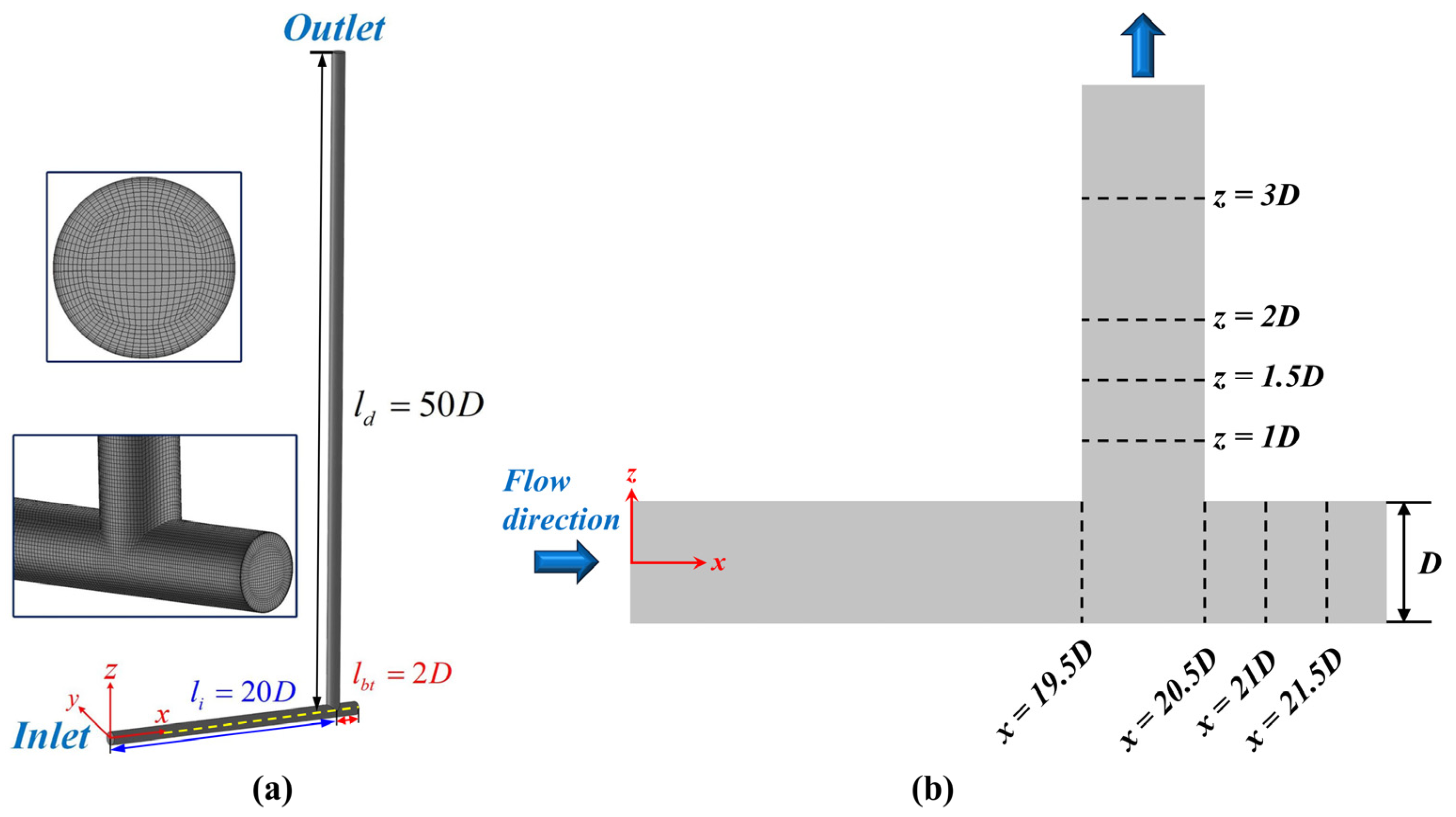
2.2. Computational Setups

Figure 1 illustrates the computational domain, featuring a straight inlet section with l_i = 20D and a straight downstream section with l_d = 50D, where the pipe diameter D is 1 m. The blind-tee length l_bt is depicted as 2D in Figure 1, which is changed from 2D to 4D to analyze its structural effect.

In the numerical simulations, a modified power law velocity distribution is set as the inlet boundary condition with a normal pressure gradient of zero. The power law profile characterizing the fully developed turbulent flow is presented as follows [39]:

$$u={\displaystyle \frac{\overline{U}}{\beta (1,1+n)}}{(1-{({\displaystyle \frac{r}{R}})}^2)}^{{\displaystyle \frac{1}{n}}}$$

(8)

where $\overline{U}$ is the average inlet velocity, β is the first kind Euler integral, n is specified as n = 0.77ln(Re) − 3.47, R denotes the pipe radius, and r signifies the radial distance from the center.

At the outlet of the pipe, a zero-pressure boundary is set, with a normal gradient of zero for the velocities. All wall surfaces are designated as non-slip boundaries. Since this study focuses on the effect of blind-tee structures on the flow-mixing mechanism, the influences of gravity and pressure are not considered in the present stage, and the buoyancy model in the simulation is set to be non-buoyant.

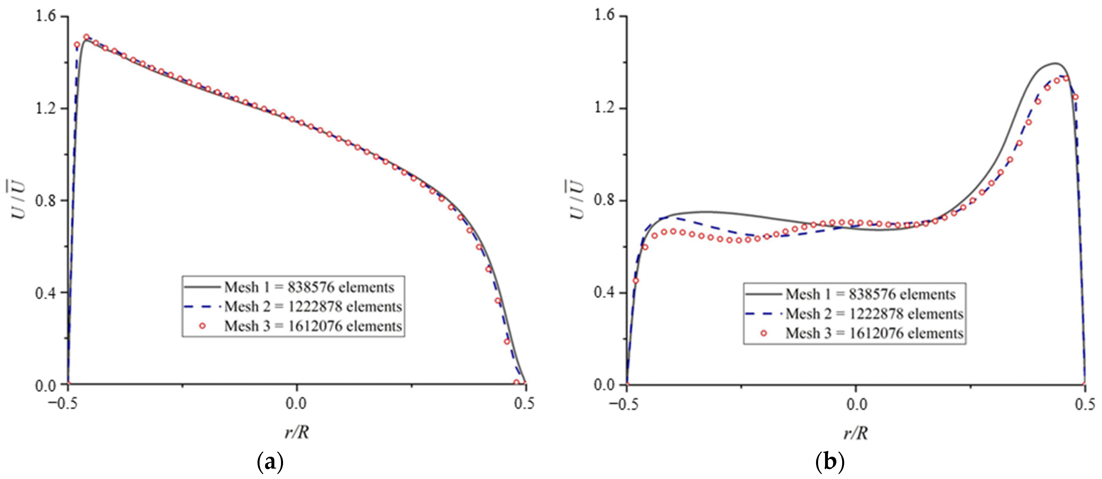
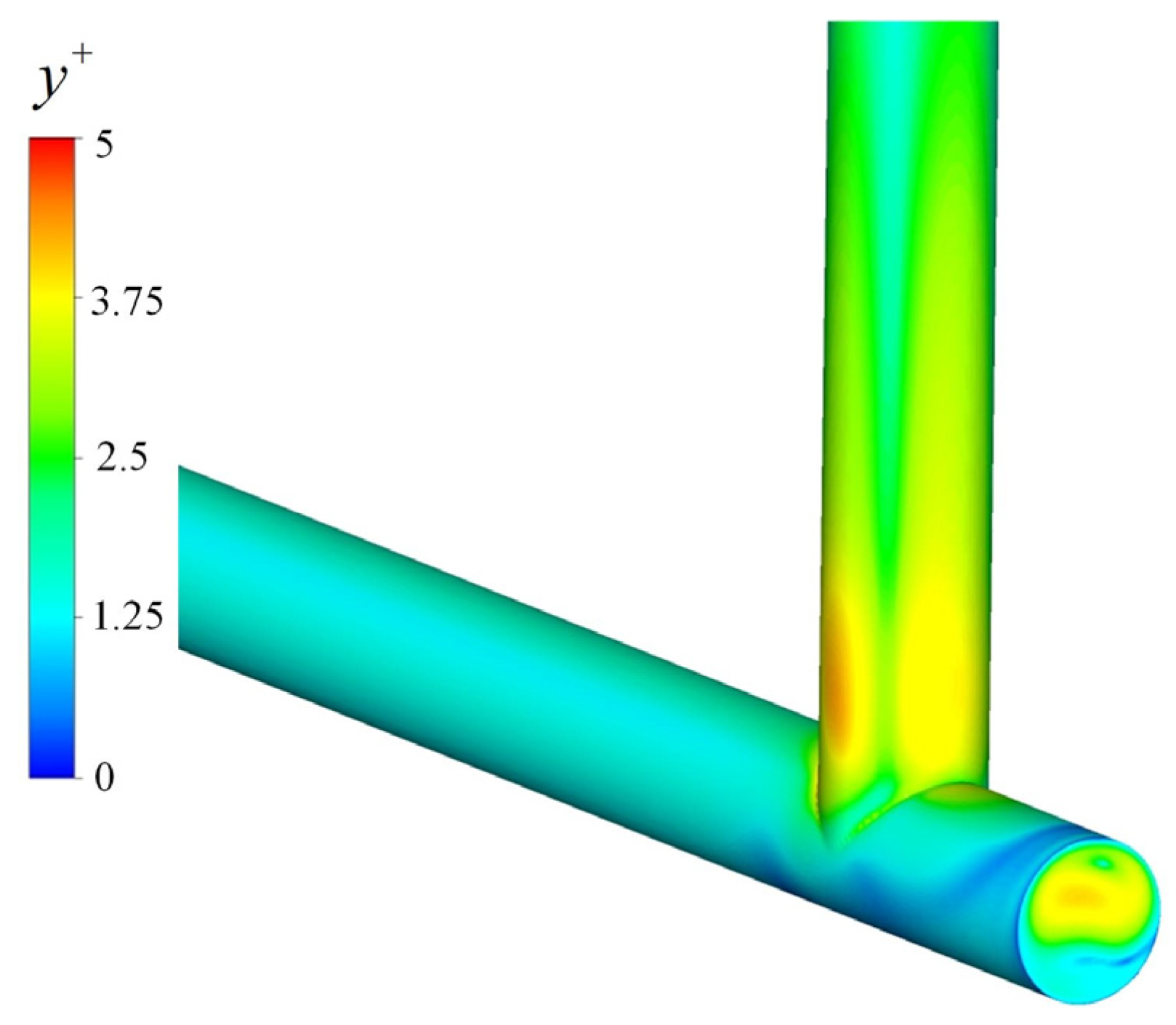
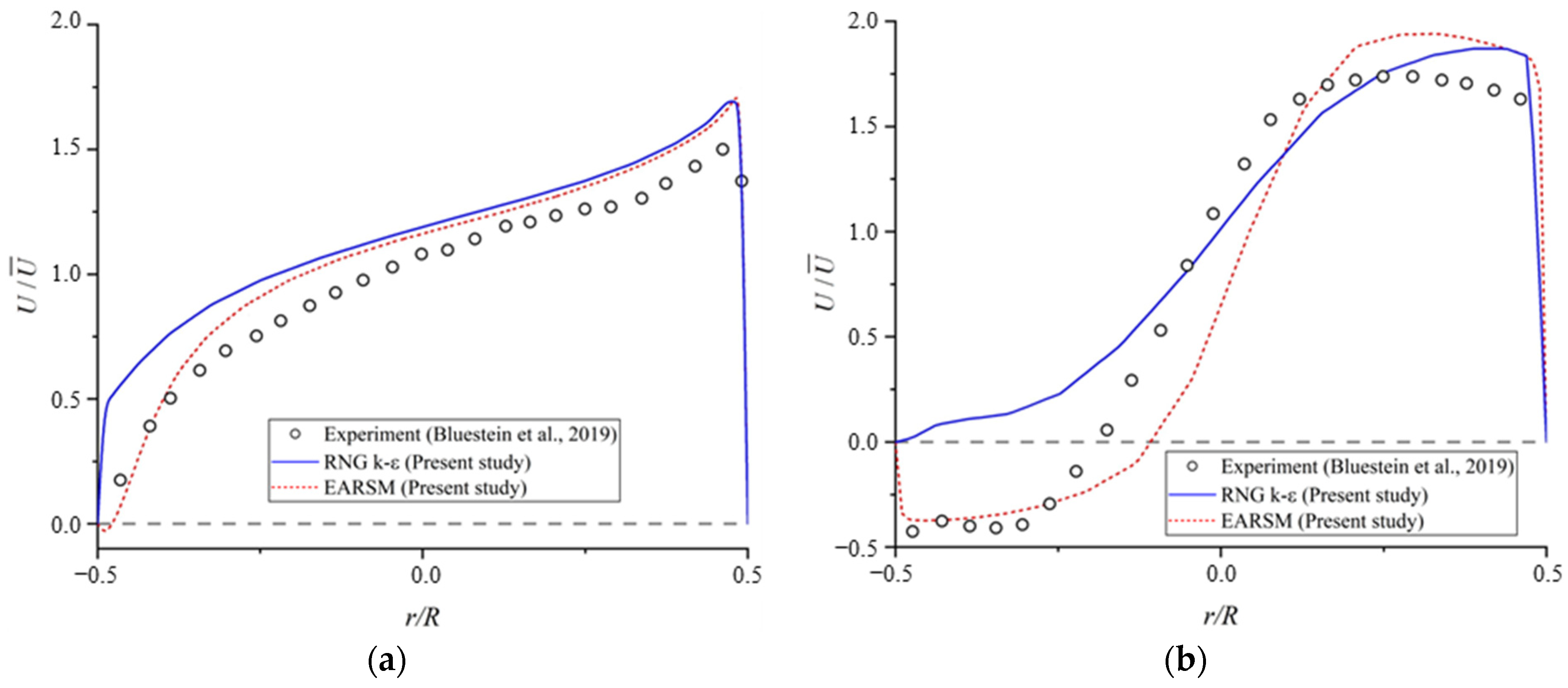
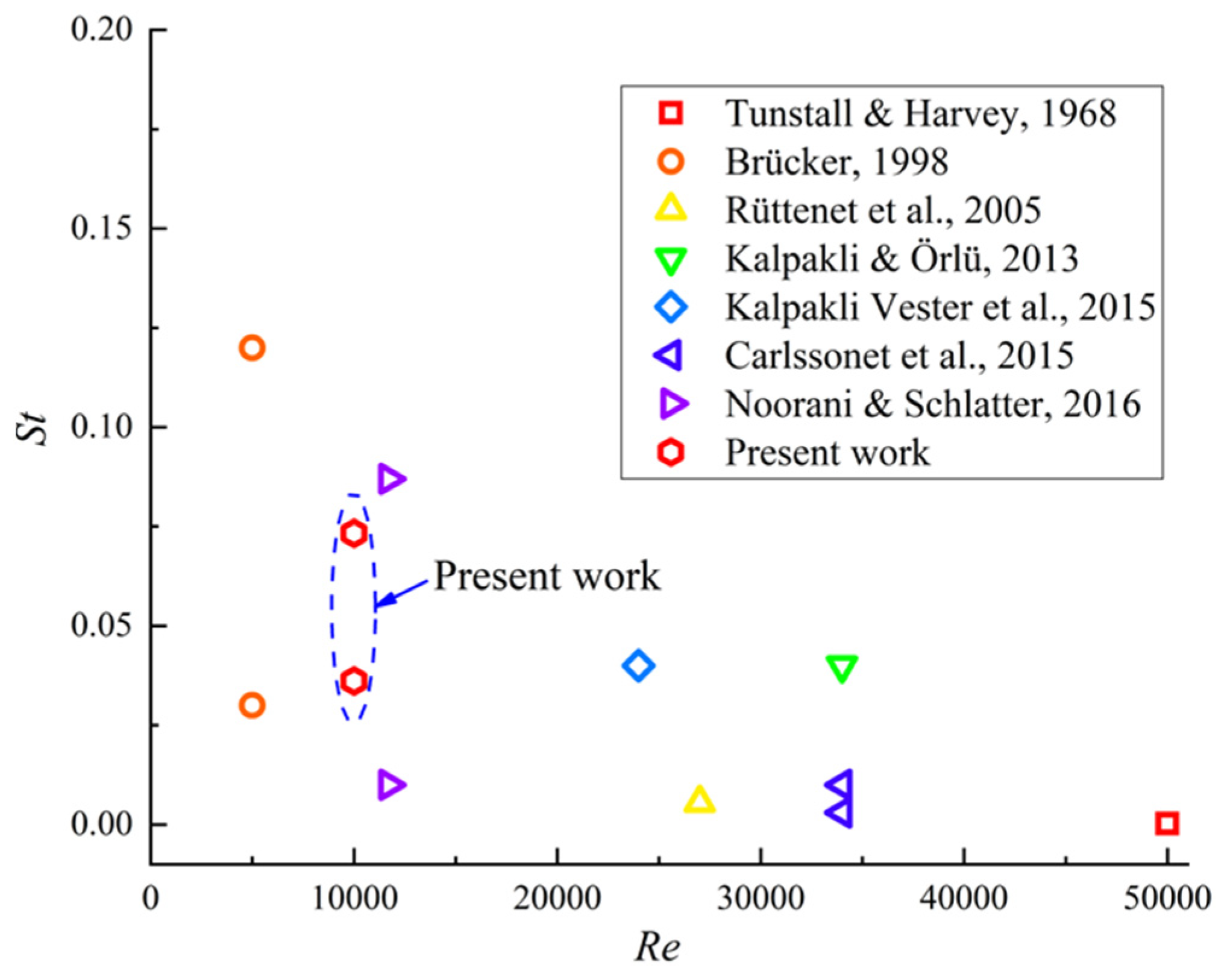
2.3. Verification and Validation

The numerical simulation’s reliability was confirmed through verification and validation processes. Firstly, the grid and time convergence analyses were conducted to determine suitable meshing and time step strategies for the simulation. Subsequently, the numerical method was validated against the experimental data reported by Bluestein et al. [34]

Three mesh configurations were developed to discretize the computational domain of the blind-tee pipe at l_bt = 2D and Re = 10,000. Velocity profiles from these three meshes were extracted at the straight inlet section (x = 19.5D) and downstream section (z = 3D), as depicted in Figure 2. The velocity distributions exhibited strong consistency at x = 19.5D across Mesh 1 (838,576 elements), Mesh 2 (1,222,878 elements), and Mesh 3 (1,612,076 elements). The average and maximum deviations in both average and maximum velocities did not exceed 1.1% and 5.7%, respectively. Similarly, at z = 3D, the average deviation between Mesh 1 and Mesh 2 was 5%, whereas the deviation between Mesh 2 and Mesh 3 was narrowed down to only 2.2%.

Moreover, the disparity peaks at over 15% between Mesh 1 and Mesh 2, while reducing notably to 7.3% between Mesh 2 and Mesh 3. Figure 3 illustrates the contour of y⁺ values derived from Mesh 2, where the maximum y⁺ value remains below 5 and the average y⁺ value stands at a mere 2.4. This indicates substantial near-wall resolution. Hence, Mesh 2 is deemed to offer a satisfactory grid resolution and is utilized for numerical simulations in this investigation.

Additionally, a time convergence analysis was executed, utilizing Mesh 2 with Courant numbers Co of 0.3, 0.6, and 0.9. This can be expressed as follows:

$$Co=\frac{1}{2}\Delta t{\displaystyle \frac{{\displaystyle {\sum }_f\left|U_f\cdot {\widehat{n}}_f\right|}{A}_f}{V}}$$

(9)

where Δt represents the time step, $U_f\cdot n_f$ represents the component of velocity vector normal to the surface of the grid, $A_f$ represents the surface area, and V is the volume of the grid. Figure 4 displays the velocity distributions at z = 2D with Co = 0.3, 0.6 and 0.9, showing good agreement among the three time-steps. Therefore, Mesh 2 with Co = 0.9 is considered to have a sufficient time-step resolution.

To further validate the credibility of the numerical model in this study, numerical results were compared with experimental data reported by Bluestein et al. [34]. Utilizing PIV, the experiment analyzed turbulent flow within a blind-tee channel featuring a square cross section at Re = 11,500. For the validation process, the computational setup closely mirrored the experimental setup, maintaining identical flow conditions. Figure 5 illustrates the axial velocity profiles derived from both numerical simulations and experimental data at two specific locations (0.5D upstream and 1.5D downstream from the blind tee), where r/R is the dimensionless radial position, to illustrate the relative locations of the results in the radial direction of the cross section. It is noteworthy that in this analysis, the RNG k-ε model is employed alongside the EARSM turbulence model for comparison.

Observations reveal that at 0.5D upstream of the blind tee, numerical outcomes from both the EARSM and RNG k-ε models generally align with the experimental data but lean towards slightly higher values. Conversely, at 1.5D downstream of the blind tee, the EARSM model effectively predicts the inner-side flow separation, near r/R = −0.5. In contrast, the RNG k-ε model produces significantly higher values and fails to capture the separation. The numerical simulation slightly overestimates velocity by 10% near the outer-side corner (i.e., r/R = 0.5), a trend also noted by Bluestein et al. [34] and attributed to experimental errors. Overall, results from the EARSM generally align with the experimental data, despite the slight discrepancy near the outer-side corner. Moreover, in contrast to the RNG k-ε model, the EARSM accurately captures near-wall flow separation using identical grid resolution. This consistency reinforces the validation of the numerical approach applied in this study.

In order to ensure the dynamic reliability of the EARSM model in predicting the vortex structures, the St numbers obtained in this study are utilized for comparison with the data from the previous studies [18,40,41,42,43,44,45]. As shown in Figure 6, the St number characterizing the vortex switching is generally distributed in the range of 0.0002–0.13 in a range of Re = 5000–50,000, and the St numbers for swirl-switching captured in this paper are 0.0361 and 0.0733. Therefore, it can be shown that the dynamic characteristics of the vortex structure captured in this paper are reasonable.

3. Results and Discussion

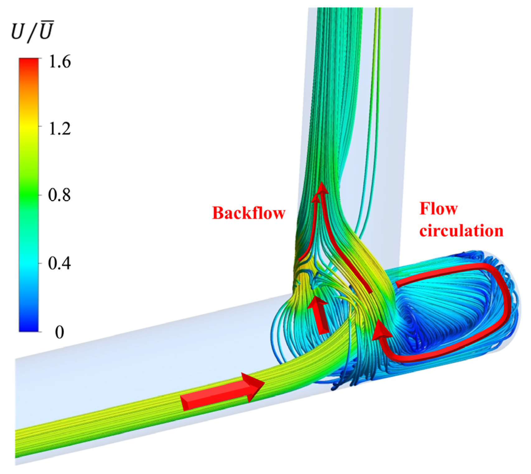
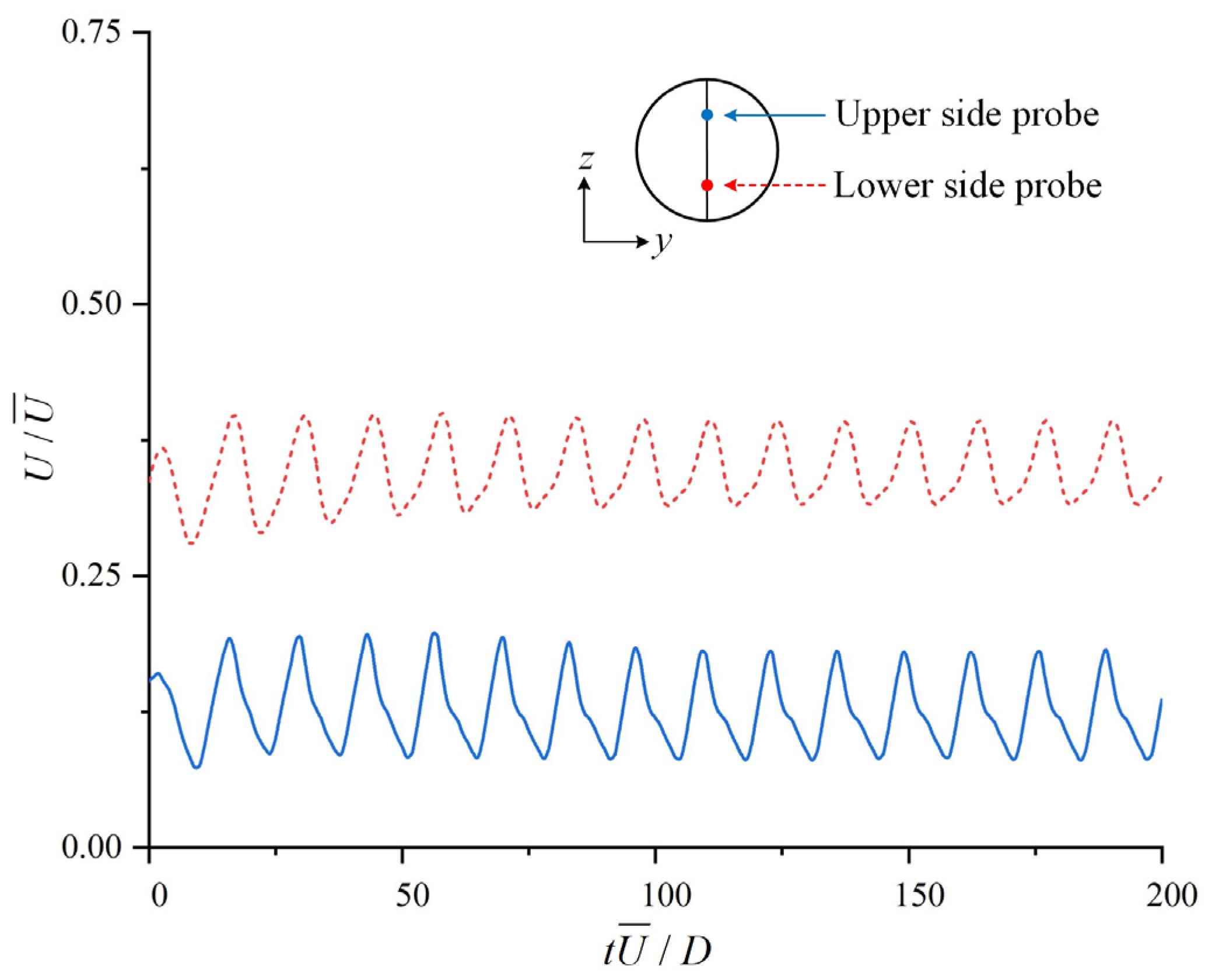
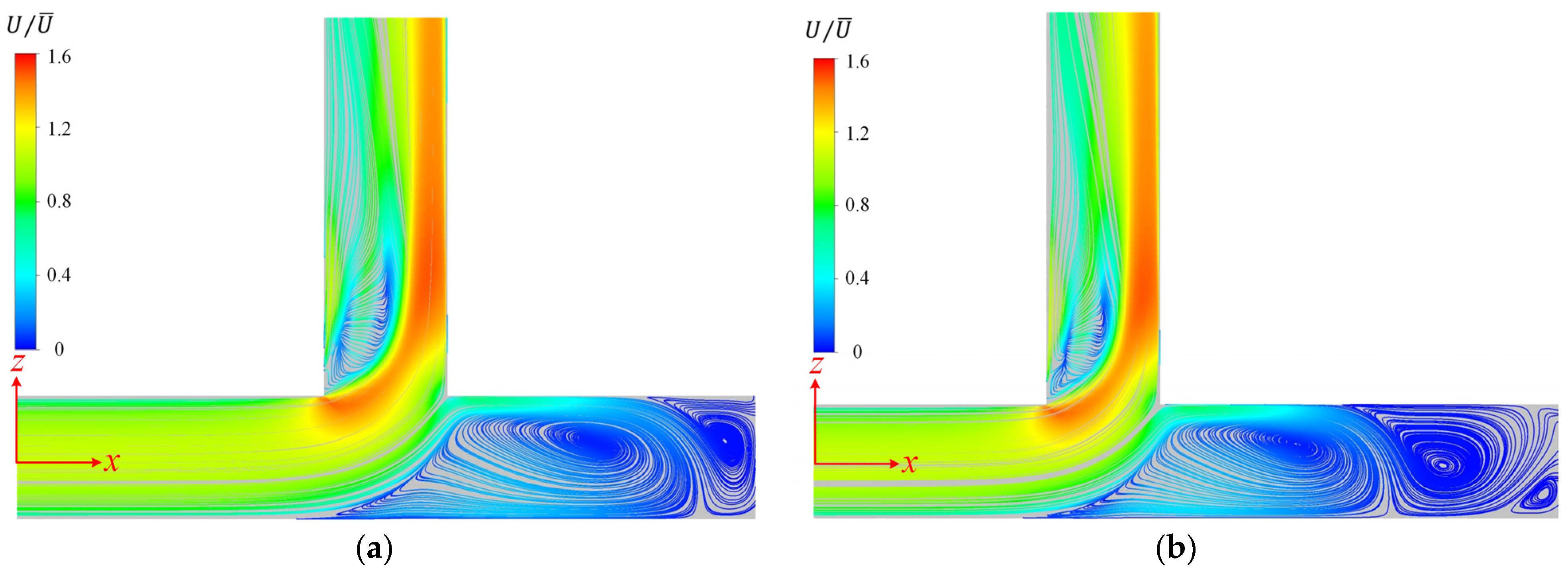
3.1. Time-Averaged Flow Characteristics

This section centers on time-averaged outcomes to analyze the statistical flow characteristics within a blind-tee pipe at Re = 10,000 and l_bt = 2D. Initially, a series of time-averaged flow patterns is presented to provide a comprehensive view of the flow dynamics. Subsequently, the intensity of secondary flow and its dissipation process are evaluated to propose potential locations for a flowmeter.

Figure 7a depicts time-averaged streamlines in the blind-tee section, emphasizing dimensionless velocity, indicated as $U/\overline{U}$. Most of the fluid flows downstream, with a portion directed towards the plugged end. Downstream flow accelerates along the outer-side corner, creating a separation zone approximately 1D–2D long near the inner-side wall. Fluid entering the plugged section encounters obstruction from the blocked end, leading to a slower outflow through the lower side. Consequently, circulation flow is established throughout the entire blind-tee section. Figure 7b shows two significant features of pressure distribution when the fluid passes through the blind tee. One is the formation of a high-pressure zone at the blind end due to the blockage effect of the blind tee. The other is that the fluid entering the pipeline downstream, due to the flow separation effect, produces a more significant pressure gradient, which also directly results in the phenomenon of the blind end of the fluid flowing back downstream.

To illustrate the backflow dynamics within the blind-tee section, three-dimensional streamlines representing the backflow are derived from the flow field and depicted in Figure 8. The analysis reveals that initially, the fluid in the plugged section mainly occupies the lower side of the pipe, eventually forming a flow cycle within this area. Subsequently, this resulting backflow reverts towards the downstream pipe, adhering to both sides of the wall due to the low-pressure zone near the inner-side corner. Moreover, Figure 9 presents axial velocity contours and cross-sectional flow velocity vector fields at specific positions (i.e., x = 20.5D, 21D, and 21.5D) to further illustrate the secondary flow patterns within the blind-tee section.

It is observed that the flow velocity entering the plugged section is nearly twice the velocity of backflow with opposite orientation. Additionally, the peak velocity does not appear at the entrance but in the middle of the plugged section. According to the cross-sectional flow velocity vector fields, most of the fluid at the upper side starts to move downwards at x = 20D and reverses the direction at x = 21.5D. Then, the backflow accelerates at x = 21D and forms a pair of counter-rotating vortices, illustrating the exchanging process of the fluid in the plugged section. Finally, the fluid turns downstream and blends with the main flow at x = 20.5D. Through the exchange of tangential momentum inside the plugged section, it is revealed that the backflow motions enhance flow mixing.

Subsequently, an investigation into the flow downstream of the blind-tee section is conducted and compared with traditional 90° elbows. To assess the strength of the swirl and its dissipation, the swirl intensity is employed to quantify the swirling flow in this study, which is defines as follows [46]:

$$I_s={\displaystyle \frac{{{\displaystyle \int [U-(U\cdot \widehat{n})\widehat{n}]}}^{2}dA}{{\overline{U}}^2{\displaystyle \int dA}}}$$

(10)

where U is the vector of flow velocity, $\widehat{n}$ is the unit vector normal to the cross section, and $\overline{U}$ is the average inlet velocity.

The curvature ratio R_c/D is commonly used to assess the bending degree of elbow pipes, where R_c is the radius of the curvature of the bend and D is the pipe diameter. Previous studies [6,11] have examined the dissipation of swirl intensity in 90-degree elbows with various curvature ratios, yielding significant insights. Their analyses indicate that the dissipation rate of swirl intensity in bent flows exhibits a weak correlation with the Reynolds number but a strong relationship with the curvature ratio. The dissipation equation for this phenomenon can be expressed as follows:

$$I_s=I_{s_0}\cdot e^{-{\beta }_s{\displaystyle \frac{l_d}{D}}}$$

(11)

where $I_{S_0}$ is the swirl intensity at the outlet of bend, ${\beta }_S$ is a variable indicating the dissipation rate, $l_d$ is the downstream distance from the bend outlet, and D is the diameter of the cross section.

The swirl intensity in a blind-tee pipe with l_bt = 2D at Re = 10,000 is extracted from the flow fields to evaluate the flow-mixing condition. According to the energy cascade mechanism, it can be seen that the enhancement of the secondary flow at the outlet of the blind tee promotes the breakdown of turbulent vortices, leading to the dissipation of turbulent energy. This results in a decrease in the swirl intensity. The variation in swirl intensity downstream of the blind tee is plotted in Figure 10 and compared with the results of 90° elbow flow under various curvature ratios R_c/D, as reported by Sudo et al. [11], Kim et al. [46] and Al-Rafai et al. [47]. It should be noted that the ordinate is given as a logarithmic scale in Figure 10 for a clear comparison. In the 90° elbow, the decreasing rate ${\beta }_s$ is nearly 0.21, with a low curvature ratio (e.g., R_c/D = 2, 3, and 3.49). This increases to 0.42 when the R_c/D is 6.975. It is found that the initial swirl-intensities $I_{s_0}$ for the flow in 90° elbows are lower than 0.1, regardless of the curvature ratio. Nonetheless, the $I_{s_0}$ value characterizing flow within a blind-tee pipe is considerably higher, being approximately an order of magnitude greater than that observed in an elbow. This emphasizes the presence of a notably intensified secondary motion within the blind-tee configuration. Furthermore, the decrease in the swirling flow in blind-tee pipes exhibits an exponential form with a coefficient ${\beta }_s$ of 2.96 at the first 2D downstream, which is about 14 times higher than the 90° elbow. The high ${\beta }_s$ implies a strong secondary motion at a short distance downstream of the bending, which is attributed to the combined influence of curvature and the plugged end. Then, the swirl intensity becomes flattened after 2D downstream. The findings validate the significant presence of a secondary flow within the blind-tee pipe and quantify the diminishment of this secondary motion. This information holds importance as it serves as a reference for determining the optimal location of flowmeters within submarine pipeline systems, steering clear of regions affected by intense cross-sectional secondary flow.

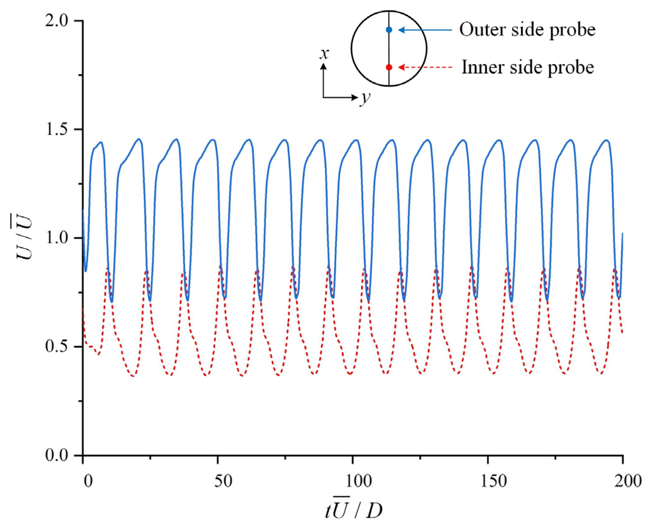
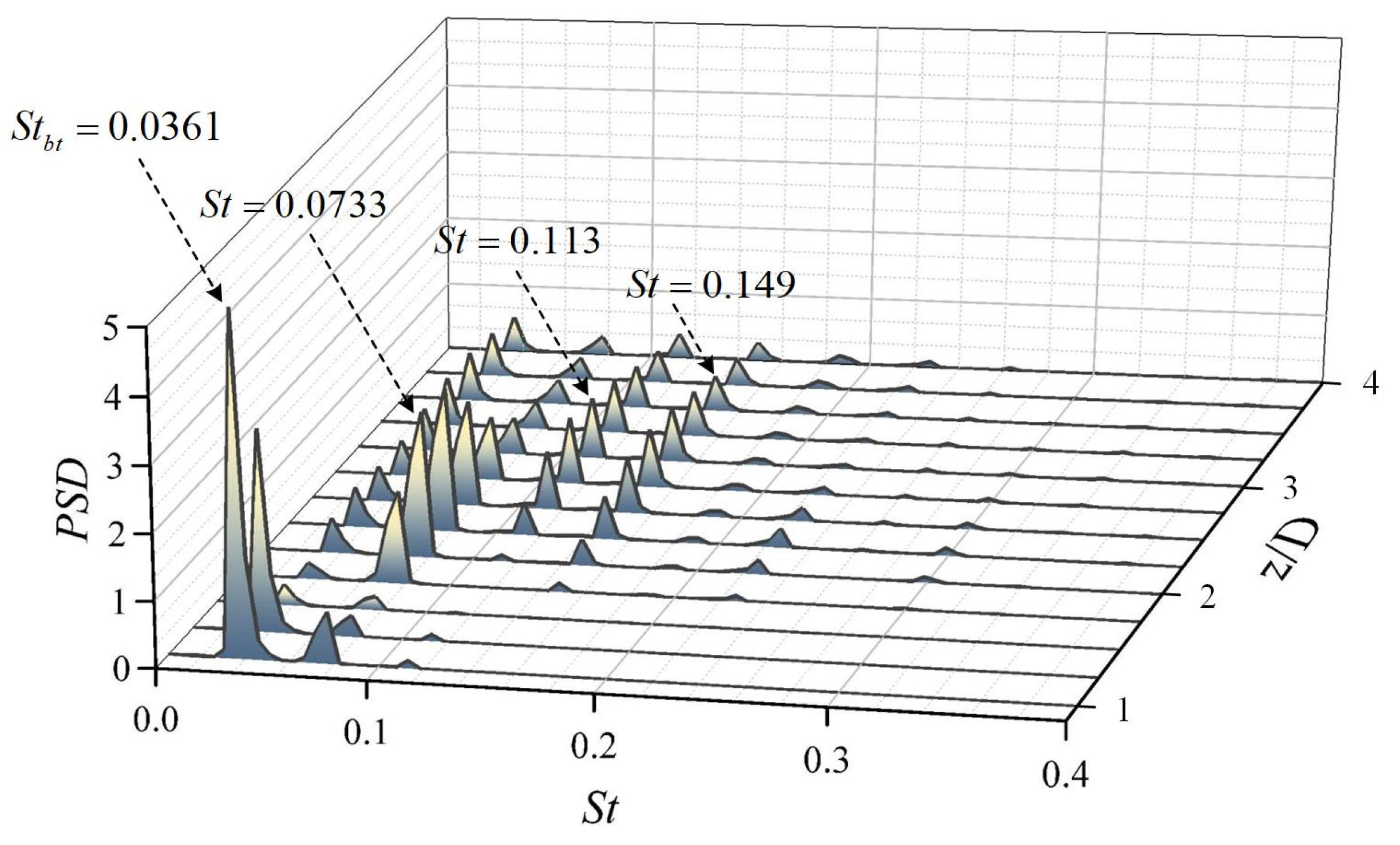
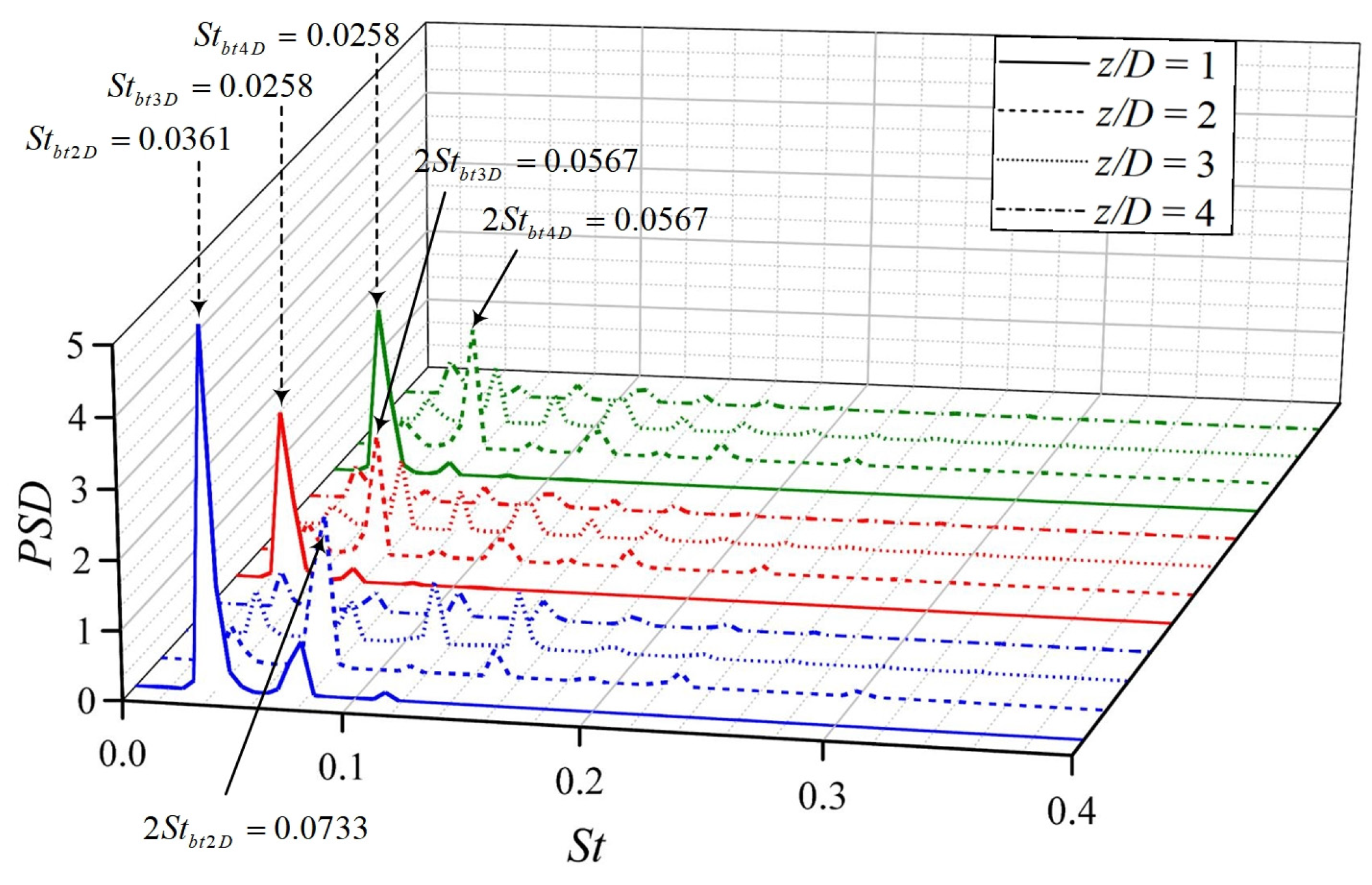
3.2. Unsteady Flow Characteristics

In this section, instantaneous flow snapshots are discussed in detail to investigate the unsteady flow characteristics in blind-tee pipes. The oscillatory patterns can not only be observed downstream but are also inside the plugged section. First, a series of flow-field snapshots in blind-tee pipes with l_bt = 2D at Re = 10,000 is obtained via numerical simulations. Then, the instantaneous flow characteristics are revealed based on the evolutions of velocity distributions, Dean motions, and the iso-surfaces of vortices. Finally, spectrum analysis is conducted to discuss the temporal features of the unsteady flow.

Using the snapshots, the unsteady flow motion downstream of the blind-tee section is recorded. Figure 11 shows the probe time sequences of velocity from $t\overline{U}/D=0 \mathrm{to} 200$ near the inner-side and outer-side corners (i.e., r/D = ±0.25) at z = 2D. A quasi-periodic pattern of flow can be observed through the probe signals, and the length of the period is estimated at 12$t\overline{U}/D$. It is found that the velocity variations at the inner-side and outer-side corners are opposite. When the flow near the inner-side corner slows down, the outer-side flow accelerates instead.

To further study the temporal evolution of secondary flow downstream of the plugged section, the cross-sectional streamlines at z = 1D and 2D in one oscillatory period (i.e., $t_0\overline{U}/D=147$, $t_1\overline{U}/D=150$, $t_2\overline{U}/D=153$, $t_3\overline{U}/D=156$, $t_4\overline{U}/D=159$,$t_5\overline{U}/D=162$, $t_6\overline{U}/D=165$, $t_7\overline{U}/D=168$, $t_8\overline{U}/D=171$) are displayed in Figure 12. It is worth noting that the streamlines are colored by the nondimensional tangential velocity $U_{t_z}/\overline{U}={(u^2+v^2)}^{\frac{1}{2}}/\overline{U}$. At z = 1D, oscillatory features can be observed based on the evolution of Dean vortices: the main pair of Dean vortices rotates nearly 60 degrees clockwise in the first three time intervals (i.e., $t_0\overline{U}/D$ to $t_3\overline{U}/D$), and then quickly resets to the initial position in one time interval (i.e., $t_3\overline{U}/D$ to $t_4\overline{U}/D$). Subsequently, the flow repeats this process anticlockwise in the next half time series (i.e., $t_4\overline{U}/D$ to $t_8\overline{U}/D$), revealing an oscillatory manner. Additionally, the strength of Dean vortices also displays a periodic manner. The tangential velocities indicate that, within one period, one of the Dean vortices is suppressed and its opposite is enhanced. The enhancing-suppressing alternation of the Dean vortices was also reported by Hellström et al. [19] in a curved channel. At z = 2D, the dynamics of Dean motions show a different pattern. Compared with that at z = 1D, the size of the vortex becomes larger. Furthermore, the magnitude of the tangential velocity is almost reduced by half, and a triple of vortices is observed with a low tangential velocity magnitude. The differences may be attributed to the rapid decrease in the swirl intensity revealed in Section 3.1.

Then, the probe time sequences of the velocity at x = 21D are shown in Figure 13 to demonstrate the unsteady properties of flow inside the plugged end. It is found that the amplitude of the velocity fluctuation inside the plugged section is much lower than that of the downstream pipe. Still, the oscillatory pattern in the plugged section can be clearly observed.

The cross-sectional streamlines of secondary flow inside the plugged section (i.e., x = 20.5D) are shown in Figure 14, colored by nondimensional tangential velocity $U_{t_x}/\overline{U}={(w^2+v^2)}^{\frac{1}{2}}/\overline{U}$. It is observed that a single vortex is generated in the period of the first to third time intervals (i.e., $t_0\overline{U}/D$ to $t_3\overline{U}/D$), moves from the pipe wall to the center, and then dissipates rapidly in the next time interval. Meanwhile, a weak vortex appears on the opposite side, and repeats the same process. The vortices from both sides of the pipe wall develop in an alternative manner inside the blind-tee section. After eight time intervals, the structure of secondary flow returns to the initial state, indicating that the secondary flow inside the plugged section also exhibits a periodic motion.

To clearly reveal this unsteady flow pattern both inside and downstream of the plugged section, Figure 15 shows the instantaneous vortex structures identified by Q-criterion [48], which can be expressed as $Q=({\Omega }^2-S^2)$. Here, Ω and S are the rotation and strain tensor, respectively. The nondimensional iso-surface $Q^{\ast }=Q{D}^2/{\overline{U}}^2=30$ is employed. It should be noted that the iso-surface of Q* is colored by the positive and negative value of y coordinate in order to display the change in the spatial location of vortex more clearly. Furthermore, the additional contours of Q* in the cross section at z = 1D are shown in the red square frame, and the corresponding color map is displayed on the right. At $t_0\overline{U}/D$, a quasi-symmetric vortex structure can be observed both inside and downstream of the plugged section. Then, the vortex in the -y direction is suppressed, and the opposite in the +y direction is enhanced in the following three time intervals (i.e., $t_0\overline{U}/D$ to $t_3\overline{U}/D$). Therefore, a deflection of the dominant vortex can be found in this process. Moreover, the vortex structure near the bending part deflects first, followed by the latter part of the whole structure. Then, the oblique vortex structure resets to the symmetry in the next time interval (i.e., $t_3\overline{U}/D$ to $t_4\overline{U}/D$). Hence, it is concluded that the dominant vortex alternates every four time intervals. For the vortex structure inside the plugged section, the oscillation manner is quite similar to that of the downstream flow. This phenomenon implies that the plugged end structure may contribute to the oscillatory manner of flow in the blind-tee pipe, and this will be further discussed in the next section.

To further investigate the oscillatory behavior of the turbulent flow inside the blind-tee pipe, power spectra analyses of the tangential velocities probe data at r/D = 0.25 were conducted on the symmetric lines at a sampling frequency of St = 1. Figure 16 shows the frequency spectra of the tangential velocity from z = 1D to 4D with l_bt = 2D at Re = 10,000. It can be seen at z = 1D that the peak value of power spectra density (PSD) corresponds to a Strouhal number of 0.0361. Hence, $S{t}_{bt}=f_{bt}\cdot D/\overline{U}=0.0361$ is considered to be the dominant frequency of the oscillatory phenomenon. When the value at the sampling position increases to z = 2D, the energy at the lowest frequency decreases rapidly, and the second harmonic St = 0.0733 dominates the flow. Then, the contribution of the second harmonic decreases in the next 2D length. At z = 3D, the flow is dominated by the third and fourth harmonics at St = 0.113 and 0.149. Therefore, it is concluded that the dominant part of the spectrum moves from a low frequency to a high frequency with the increase in z/D. Moreover, both low- and high-frequency components make equal contributions to the flow further downstream (e.g., z ≥ 3D), while the spectrum at z = 1D is concentrated in the two lowest frequencies. The change in the dominant frequency may be due to the dissipation of the large-scale vortices, which is also revealed in the evolution of Dean motions, shown in Figure 12.

As a comparison, the frequency spectra of the tangential velocities probe data at selected position inside the section (i.e., r/D = 0.25 on the symmetric line from x = 20.5D to 21.5D) are given in Figure 17. The spectra indicate that St_bt = 0.0361 is also the dominant Strouhal number characterizing the unsteady flow inside blind-tee section revealing a strong correlation between the flow inside and downstream of the plugged section. In addition, the second and third harmonics St = 0.0733 and 0.113 also contribute to the flow inside the plugged section. Compared with the study on turbulent flow in a sharp bend (i.e., l_bt = 0) by Tunstall and Harvey [18] the Strouhal number St_bt = 0.0361 of the oscillatory phenomena in blind-tee pipes is much higher than the value in a sharp bend, which shows a stronger swirl switching process. Therefore, it is concluded that the plugged end structure contributes to the oscillatory patterns by enhancing the flow-mixing conditions. This structural effect will be further discussed in Section 3.3.

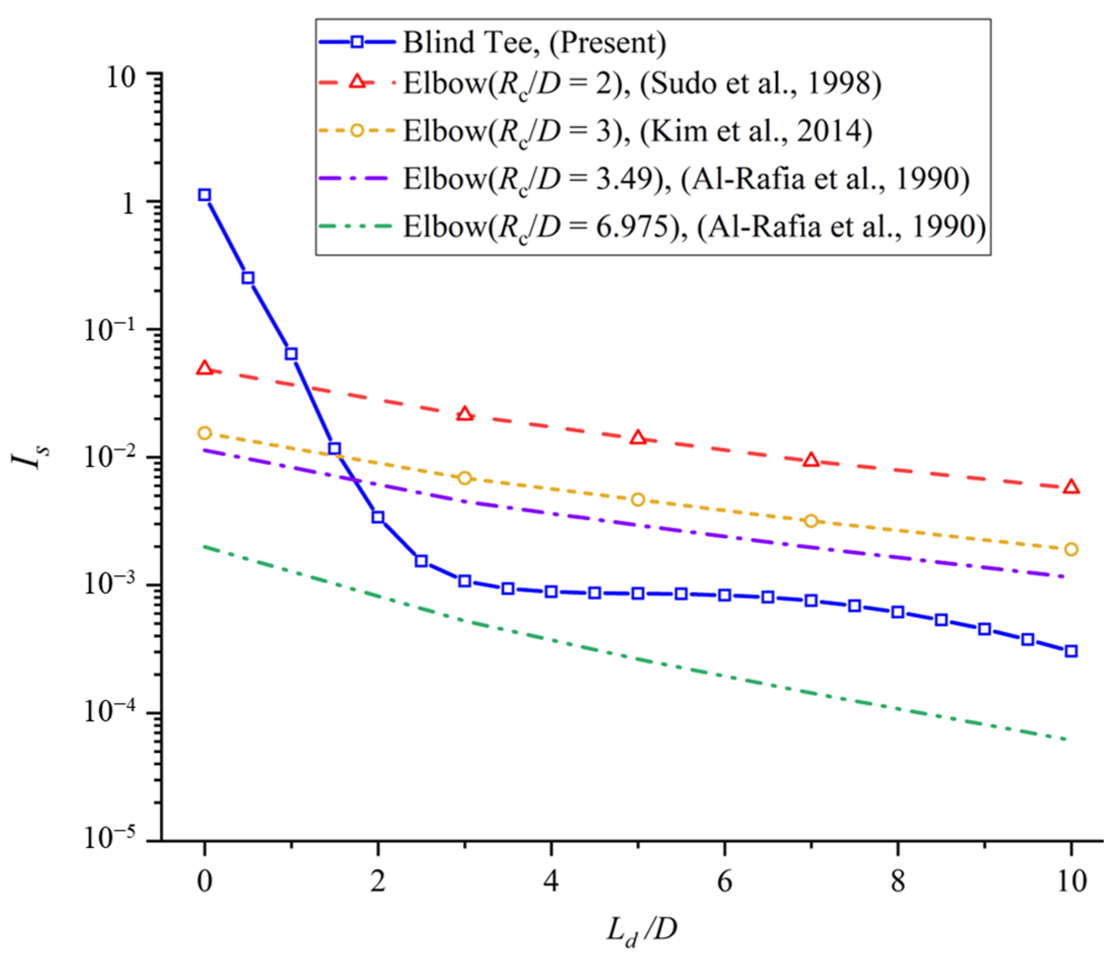
3.3. Structural Effect

This section investigates the influence of blind-tee length (l_bt) on the flow characteristics within the blind-tee pipe. Illustrated in Figure 18 are the time-averaged streamlines of the symmetry plane for l_bt = 3D and 4D. Compared with the streamlines with l_bt = 2D, shown in Figure 7, an additional flow circulation is observed near the plugged end in Figure 18a, induced by a bifurcation near the middle of the plugged section. This additional flow circulation exhibits relatively minor velocity and opposes the main circulation. The main circulation spans approximately 2D in length, while the supplementary circulation encompasses only about 1D in length. With l_bt increasing to 4D, a third flow circulation occurs near the end corner with low velocity. Furthermore, the downstream flow of blind-tee sections in Figure 18a,b appears to be similar despite the different blind-tee lengths. This similarity arises because the flow near the plugged end is nearly stagnant, implying that the extra two flow circulations with low velocity have little influence on the downstream flow field. In other words, the effective length of the blind tee is less than 3D.

To explore how the l_bt affects unsteady flow dynamics, Figure 19 depicts the frequency spectra of tangential velocity downstream from z = 1D to 4D, considering l_bt = 2D, 3D, and 4D. It is worth noting that the downstream distances are separated by the line types and the different blind-tee structures are separated by the colors. For l_bt = 3D and 4D, the dominant frequencies are the same (i.e., St_bt3D = St_bt4D = 0.0258), but lower than that in l_bt = 2D. Therefore, the periodic length of the oscillatory pattern in l_bt = 3D and 4D is longer than that in l_bt = 2D. With the increase in z/D, the second and third harmonic dominate the unsteady flow. Moreover, it can be observed that the frequency spectra from z = 1D to 4D with l_bt = 3D and 4D are very similar, indicating the analogous oscillatory process.

Subsequently, the frequency spectra of tangential velocity inside the plugged section are plotted in Figure 20. Due to the different plugged section lengths, the detected positions are from x = 20.5D to 21.5D, from 20.5D to 22.5D and from 20.5D to 23.5D in l_bt = 2D, 3D and 4D, respectively. The frequency spectra of l_bt = 3D and 4D are very similar, and the dominant frequencies are both 0.0258, which are lower than those of l_bt = 2D. It is found that the second harmonic (i.e., 2St_bt3D = 2St_bt4D = 0.0567) dominates the flow at the entrance of plugged sections (i.e., x = 20.5D) in l_bt = 3D and 4D. Then, it decreases to 0.0258 in the next 2D, indicating a lower-frequency motion as the flow approaches the plugged end. Furthermore, near the plugged end in l_bt = 4D (i.e., x = 23D to 23.5D), the unsteady phenomenon disappears. It means that the fluid exchange near the plugged end in l_bt = 4D is suppressed. Compared to the configurations with l_bt = 3D and 4D, the blind-tee section with a length of 2D demonstrates notably stronger tangential momentum. Moreover, the oscillatory patterns observed inside the blind-tee section of l_bt = 2D appear more pronounced than those in the other two cases.

To sum up, the increasing blind-tee section (i.e., l_bt ≥ 3D) may not influence the downstream flow behaviors, which is consistent with the time-averaged results. The l_bt = 2D is considered to provide a beneficial mixing condition, which is suggested for use in the design of blind-tee structures.

4. Conclusions

In this study, numerical simulations are employed to scrutinize turbulent flow characteristics within blind-tee pipes, a vital component of ocean engineering systems. Initially, a comprehensive analysis of time-averaged flow in a specific blind-tee pipe is conducted, employing streamlines and vector fields to depict average flow behaviors. Moreover, the decrease in swirl intensity is extracted from the flow fields and compared with the 90° bend flow data derived from the published literature, thus providing valuable insights. Subsequently, unsteady flow characteristics are systematically investigated through time–frequency domain analysis on a series of flow-field snapshots, revealing oscillating flow motions inside and downstream of the plugged section. Additionally, the influence of blind-tee length is discussed, leading to the identification of an optimized structure for enhanced flow mixing. In conclusion, this study sheds light on critical aspects of turbulent flow within blind-tee pipes, offering valuable insights for the design and optimization of ocean engineering systems.

(1) The analysis of the time-averaged flow field reveals a flow cycle, occupying the entire plugged section. Backflow originating from the plugged end generates opposing rotating vortices, thereby enhancing fluid exchange within the blind tee. Downstream flow exhibits an initial swirl intensity which is significantly higher than that observed in a 90° elbow, indicating favorable fluid exchange conditions in the blind-tee pipe. Enhancing the secondary flows at the outlet of a blind tee promotes the breakdown of turbulent vortices, leading to the dissipation of turbulent energy. Hence, the decreasing rate of swirl intensity varies exponentially within the 2D length downstream of the blind-tee section, being approximately 14 times higher than that in the 90°elbow. However, this decreasing rate rapidly decreases when L_d > 2D. Consequently, to avoid the violent swirl region, it is recommended to place the flowmeter after a downstream distance of 2D from the plugged section.

(2) The oscillatory manners of turbulent flow in the blind-tee pipe with l_bt = 2D are revealed to enhance the flow-mixing condition, and the periodic Dean motions are displayed using snapshots of secondary flows. Furthermore, the nondimensional dominant frequency is obtained as St_bt = 0.0361, both inside and downstream of the plugged section. This is ten times higher than that of the sharp-bent flow (i.e., l_bt = 0D). It indicates that the oscillatory patterns between the flows inside and downstream of the blind-tee section are highly related, and the plugged end structure is a critical factor in the oscillatory movements.

(3) Structural modifications result in additional low-speed flow circulations near the plugged end when the blind-tee length surpasses 3D. However, despite further increases in blind-tee length, flow behaviors remain relatively consistent. This suggests that the effective length of the blind tee, significantly influencing downstream flow, is limited to no more than 3D. The comparison of power spectra indicates that turbulent flow within the blind tee at 2D length achieves a higher dominant frequency, offering more favorable flow-mixing conditions.

This study develops an in-depth understanding of the mixing mechanism of turbulent flow inside blind tees, illustrates the unsteady flow characteristics, and explores the time–frequency relationship between the flow circulation inside the blind end and the secondary flow downstream of the bend. The results of this paper provide new insights and ideas regarding the mixing effects and flow control methods of bending structures in offshore oil and gas pipeline systems.

References

1. Taibi, R.; Yin, G.; Ong, M.C. CFD investigation of internal elbow pipe flows in laminar regime. In Proceedings of the 3rd Conference of Computational Methods & Ocean Technology (COTech 2021), Stavanger, Norway, 25–26 November 2021. [Google Scholar]
2. Garcia, C.; Nemoto, R.; Pereyra, E.; Korelstein, L.; Sarica, C. Hydrodynamic forces in a horizontal-horizontal elbow in a gas-liquid system. Int. J. Multiphase Flow 2023, 159, 104321. [Google Scholar] [CrossRef]
3. Dean, W.R. Fluid motion in a curved channel. Proc. R. Soc. Lond. A 1928, 121, 402–420. [Google Scholar]
4. Winters, K.H. A bifurcation study of laminar flow in a curved tube of rectangular cross-section. J. Fluid Mech. 1987, 180, 343–369. [Google Scholar] [CrossRef]
5. Bara, B.; Nandakumar, K.; Masliyah, J.H. An experimental and numerical study of the Dean problem: Flow development towards two-dimensional multiple solutions. J. Fluid Mech. 1992, 244, 339–376. [Google Scholar] [CrossRef]
6. Herreros, I.; Hochberg, D. Chiral symmetry breaking and entropy production in Dean vortices. Phys. Fluids 2023, 35, 043614. [Google Scholar] [CrossRef]
7. Kim, M.; Borhan, A. Critical conditions for development of a second pair of Dean vortices in curved microfluidic channels. Phys. Rev. E 2023, 107, 055103. [Google Scholar] [CrossRef] [PubMed]
8. Wang, K.; He, Z.; Cheng, Z.; Kim, H.B. Effects of Reynolds number on dean vortices flow of a 180° curved pipe by using PIV measurements. J. Vis. 2023, 26, 743–754. [Google Scholar] [CrossRef]
9. Shui, C.; Zhou, D.; Wu, Z.; Yu, W.; Zhang, L.; Xing, T.; Wang, C.; Du, Z. Short-term operation optimization for natural gas pipeline considering line-pack: A perspective of optimal transport. Gas Sci. Eng. 2023, 117, 205075. [Google Scholar] [CrossRef]
10. Shehata, M.F.; El-Shamy, A.M. Hydrogen-based failure in oil and gas pipelines a review. Gas Sci. Eng. 2023, 115, 204994. [Google Scholar] [CrossRef]
11. Sudo, K.; Sumida, M.; Hibara, H. Experimental investigation on turbulent flow in a circular-sectioned 90-degree bend. Exp. Fluid 1998, 25, 42–49. [Google Scholar] [CrossRef]
12. Sudo, K.; Sumida, M.; Hibara, H. Experimental investigation on turbulent flow in a square-sectioned 90-degree bend. Exp. Fluids 2001, 30, 246–252. [Google Scholar] [CrossRef]
13. Jurga, A.P.; Janocha, M.; Yin, G.; Ong, M.C. Numerical simulations of turbulent flow through a 90-degree pipe bend. J. Offshore Mech. Arct. Eng. 2022, 144, 061801. [Google Scholar] [CrossRef]
14. Han, F.; Liu, Y.; Lan, Q.; Li, W.; Wang, Z. CFD investigation on secondary flow characteristics in double-curved subsea pipelines with different spatial structures. J. Mar. Sci. Eng. 2022, 10, 1264. [Google Scholar] [CrossRef]
15. Kumar, A.A.; Mathur, A.; Gerritsma, M.; Komen, E. Design of a Direct numerical Simulation of flow and heat transfer in a T-junction. Nucl. Eng. Des. 2023, 410, 112403. [Google Scholar] [CrossRef]
16. Zhang, H.; Wang, P.; Liu, H.; Wang, B.; Liu, Y. Unsteady flow behaviors and flow-induced noise characteristics in a closed branch T-junction. Phys. Fluids 2024, 36, 065148. [Google Scholar] [CrossRef]
17. Lan, Q.; Han, F.; Liu, Y.; Li, W.; Wang, Z. Numerical investigation on turbulent flow in blind tees. In Proceedings of the 2022 IEEE 17th Conference on Industrial Electronics and Applications (ICIEA), Chengdu, China, 16–19 December 2022; pp. 156–161. [Google Scholar]
18. Tunstall, M.J.; Harvey, J.K. On the effect of a sharp bend in a fully developed turbulent pipe-flow. J. Fluid Mech. 1968, 34, 595–608. [Google Scholar] [CrossRef]
19. Hellström, L.H.; Zlatinov, M.B.; Cao, G.; Smits, A.J. Turbulent pipe flow downstream of a bend. J. Fluid Mech. 2013, 735, R7. [Google Scholar] [CrossRef]
20. Sarkodie, K.; Fergusson-Rees, A.; Asiedu, N.Y. Improved phase fraction measurement via non-intrusive optical sensing for vertical upward gas-liquid flow. Gas Sci. Eng. 2023, 114, 204948. [Google Scholar] [CrossRef]
21. Liu, A.; Xu, C.; Lu, X.; Zhou, X.; Xu, W. Coupling effect of multiple factors on the diffusion behavior of leaking natural gas in utility tunnels: A numerical study and PIV experimental validation. Gas Sci. Eng. 2023, 118, 205086. [Google Scholar] [CrossRef]
22. Hufnagel, L.; Canton, J.; Örlü, R.; Marin, O.; Merzari, E.; Schlatter, P. The three-dimensional structure of swirl-switching in bent pipe flow. J. Fluid Mech. 2018, 835, 86–101. [Google Scholar]
23. Luo, M.; Jia, G.; Yang, Y.; Si, X.; Ge, Y.; Zhan, Y.; Lu, M. Numerical simulation of proppant transportation and placement in several complex structure fractures of a shale reservoir using a CFD approach. Gas Sci. Eng. 2023, 118, 205115. [Google Scholar] [CrossRef]
24. De Rosis, A.; Tafuni, A. A phase-field lattice Boltzmann method for the solution of water-entry and water-exit problems. Comput.-Aided Civ. Infrastruct. Eng. 2022, 37, 832–847. [Google Scholar] [CrossRef]
25. Li, W.; Song, W.; Yin, G.; Ong, M.C.; Han, F.H. Flow regime identification in the subsea jumper based on electrical capacitance tomography and convolution neural network. Ocean Eng. 2022, 266, 113152. [Google Scholar] [CrossRef]
26. Lu, P.; Zhao, L.; Zheng, N.; Liu, S.; Li, X.; Zhou, X.; Yan, J. Progress and prospect of flow phenomena and simulation on two-phase separation in branching T-junctions: A review. Renew. Sustain. Energy Rev. 2022, 167, 112742. [Google Scholar] [CrossRef]
27. Liu, Z.; Zhang, C.; Pang, Y.; Liu, W.; Wang, X. Dynamics of droplet breakup in unilateral Y-junctions with different angles. J. Ind. Eng. Chem. 2022, 112, 46–57. [Google Scholar] [CrossRef]
28. Liu, Y.; Han, F.; Zhang, H.; Wang, D.; Wang, Z.; Li, W. Numerical simulation of internal flow in jumper tube with blind tee. In Proceedings of the 2021 IEEE 16th Conference on Industrial Electronics and Applications (ICIEA), Chengdu, China, 1–4 August 2021; pp. 363–368. [Google Scholar]
29. Razali, M.A.B.; Xie, C.G.; Loh, W.L. Experimental investigation of gas-liquid flow in a vertical venturi installed downstream of a horizontal blind tee flow conditioner and the flow regime transition. Flow Meas. Instrum. 2021, 80, 101961. [Google Scholar] [CrossRef]
30. Li, W.; Li, J.; Yin, G.; Ong, M.C. Experimental and numerical study on the slug characteristics and flow-induced vibration of a subsea rigid M-shaped jumper. Appl. Sci. 2023, 13, 7504. [Google Scholar] [CrossRef]
31. Han, F.; Ong, M.C.; Xing, Y.; Li, W. Three-dimensional numerical investigation of laminar flow in blind-tee pipes. Ocean Eng. 2020, 217, 107962. [Google Scholar] [CrossRef]
32. Han, F.; Liu, Y.; Ong, M.C.; Yin, G.; Li, W.; Wang, Z. CFD investigation of blind-tee effects on flow mixing mechanism in subsea pipelines. Eng. Appl. Comput. Fluid Mech. 2022, 16, 1395–1419. [Google Scholar] [CrossRef]
33. Liu, Y.; Han, F.; Yin, G.; Ong, M.C.; Li, W.H.; Wang, Z. Numerical investigation of blind-tee effect on flow mixing in double-bend combinations. Ocean Eng. 2023, 287, 115909. [Google Scholar] [CrossRef]
34. Bluestein, A.M.; Venters, R.; Bohl, D.; Helenbrook, B.T.; Ahmadi, G. Turbulent Flow Through a Ducted Elbow and Plugged Tee Geometry: An Experimental and Numerical Study. J. Fluids Eng. 2019, 141, 081101. [Google Scholar] [CrossRef]
35. Wallin, S. Engineering Turbulence Modeling for CFD with a Focus on Explicit Algebraic Reynolds Stress Models. Ph.D. Thesis, Royal Institute of Technology, Stockholm, Sweden, 2000. [Google Scholar]
36. Ricci, F.; Vacondio, R.; Tafuni, A. Direct numerical simulation of three-dimensional isotropic turbulence with smoothed particle hydrodynamics. Phys. Fluids 2023, 35, 065148. [Google Scholar] [CrossRef]
37. Louda, P.; Kozel, K.; Příhoda, J.; Beneš, L.; Kopáček, T. Numerical solution of incompressible flow through branched channels. Comput. Fluids 2011, 46, 318–324. [Google Scholar] [CrossRef]
38. ANSYS Inc. ANSYS CFX-Solver Guide, 2012. Release 14.5; ANSYS Inc.: Canonsburg, PA, USA, 2012. [Google Scholar]
39. Salama, A. Velocity Profile Representation for Fully Developed Turbulent Flows in Pipes: A Modified Power Law. Fluids 2021, 6, 369. [Google Scholar] [CrossRef]
40. Brücker, C. A time-recording DPIV-study of the swirl switching effect in a 90° bend flow. In Proceedings of the Eight International Symposium on Flow Visualization, Sorrento, Italy, 1–4 September 1998; pp. 171.1–171.6. [Google Scholar]
41. Rütten, F.; Schröder, W.; Meinke, M. Large-eddy simulation of low frequency oscillations of the Dean vortices in turbulent pipe bend flows. Phys. Fluids 2005, 17, 035107. [Google Scholar] [CrossRef]
42. Kalpakli, A.; Örlü, R. Turbulent pipe flow downstream a 90° pipe bend with and without superimposed swirl. Int. J. Heat Fluid Flow 2013, 41, 103–111. [Google Scholar] [CrossRef]
43. Kalpakli Vester, A.; Örlü, R.; Alfredsson, P.H. POD analysis of the turbulent flow downstream a mild and sharp bend. Exp. Fluids 2015, 56, 57. [Google Scholar] [CrossRef]
44. Carlsson, C.; Alenius, E.; Fuchs, L. Swirl switching in turbulent flow through 90° pipe bends. Phys. Fluids 2015, 27, 085112. [Google Scholar] [CrossRef]
45. Noorani, A.; Schlatter, P. Swirl-switching phenomenon in turbulent flow through toroidal pipes. Int. J. Heat Fluid Flow 2016, 61, 108–116. [Google Scholar] [CrossRef]
46. Kim, J.; Yadav, M.; Kim, S. Characteristics of secondary flow induced by 90-degree elbow in turbulent pipe flow. Eng. Appl. Comput. Fluid Mech. 2014, 8, 229–239. [Google Scholar] [CrossRef]
47. Al-Rafai, W.N.; Tridimas, Y.D.; Woolley, N.H. A study of turbulent flows in pipe bends. Proc. Inst. Mech. Eng. Pt. C J. Mechan. Eng. Sci. 1990, 204, 399–408. [Google Scholar] [CrossRef]
48. Kolář, V.; Šístek, J. Disappearing vortex problem in vortex identification: Non-existence for selected criteria. Phys. Fluids 2022, 34, 071704. [Google Scholar] [CrossRef]
Figure 1. (a) Computational domain and (b) locations of cross sections for flow analysis.
Jmse 12 01199 g001
Figure 2. Velocity distributions at (a) x = 19.5D and (b) z = 3D with different grid resolutions at Re = 10,000.
Jmse 12 01199 g002
Figure 3. Contour of y+ value obtained by Mesh 2.
Jmse 12 01199 g003
Figure 4. Comparison of time convergence study at z = 2D.
Jmse 12 01199 g004
Figure 5. Validations of numerical results against previous experimental data [34] at (a) 0.5D upstream and (b) 1.5D downstream of the blind tee.
Jmse 12 01199 g005
Figure 6. Comparison of St numbers obtained in the previous literature [18,40,41,42,43,44,45] and the present study.
Jmse 12 01199 g006
Figure 7. (a) Streamlines and (b) pressure contour on the symmetry plane of blind-tee pipe with lbt = 2D at Re = 10,000.
Jmse 12 01199 g007
Figure 8. Three-dimensional streamlines of backflow in the blind-tee pipe with lbt = 2D.
Jmse 12 01199 g008
Figure 9. Axial velocity contours and vectors inside the blind-tee section.
Jmse 12 01199 g009
Figure 10. Comparison of the swirl intensity dissipation in the blind-tee pipe to the previous results in 90° elbows with different curvatures [11,46,47].
Jmse 12 01199 g010
Figure 11. Probe time sequences of the velocity at z = 2D.
Jmse 12 01199 g011
Figure 12. Instantaneous secondary flow at z = 1D and 2D.
Jmse 12 01199 g012
Figure 13. Probe time sequences of the velocity at x = 21D.
Jmse 12 01199 g013
Figure 14. Instantaneous secondary flow at x = 20.5D.
Jmse 12 01199 g014
Figure 15. Instantaneous vortex structures.
Jmse 12 01199 g015
Figure 16. The spectra of tangential velocity from z = 1D to 4D.
Jmse 12 01199 g016
Figure 17. The spectra of tangential velocity from x = 20.5D to 21.5D.
Jmse 12 01199 g017
Figure 18. Time-averaged streamlines on symmetry plane with (a) lbt = 3D and (b) lbt = 4D.
Jmse 12 01199 g018
Figure 19. The spectra of tangential velocity downstream of the blind-tee sections with lbt = 2D (blue), 3D (red) and 4D (green).
Jmse 12 01199 g019
Figure 20. The spectra of tangential velocity with lbt = 2D (blue), 3D (red) and 4D (green).
Jmse 12 01199 g020
Disclaimer/Publisher’s Note: The statements, opinions and data contained in all publications are solely those of the individual author(s) and contributor(s) and not of MDPI and/or the editor(s). MDPI and/or the editor(s) disclaim responsibility for any injury to people or property resulting from any ideas, methods, instructions or products referred to in the content.