Distributed Estimator-Based Containment Control for Multi-AUV Systems Subject to Input Saturation and Unknown Disturbance

Abstract

This article addresses the containment control issue for multi-AUV systems with the intervention of both external disturbance and input saturation. Firstly, a distributed estimator is established for the sake of acquiring precise estimation information of the desired position and its derivative for each follower AUV in the system. Next, on the basis of the proposed distributed estimator, a virtual control law is designed for each follower AUV. Then, due to the difficulty in obtaining accurate information about the derivative of the virtual control law, a linear tracking differentiator is introduced. Additionally, a disturbance observer is employed to tackle the composite disturbance, which mainly contains the internal model uncertainties and external bounded disturbances. Meanwhile, the issue of input saturation is handled by constructing the auxiliary system. Furthermore, a containment control law is designed with the assistance of the introduced linear tracking differentiator, the established disturbance observer, and the constructed auxiliary system. Additionally, the Lyapunov stability theory is applied to analyze the stability of the multi-AUV system. Finally, simulation results are given to confirm the feasibility of the proposed containment control scheme.

1. Introduction

With the development of science and technology, countries are paying increasing attention to the ocean field. At the same time, many marine tools have been developed [1,2,3]. Autonomous underwater vehicles (AUVs) are cable-free and unmanned marine equipment that can independently complete operational tasks based on the resources they carry [4,5]. With advantages such as an unrestricted activity range, good concealment, large operating range, high safety, and low cost, AUVs have gradually become a crucial instrument for ocean exploration and monitoring and military theater maritime reconnaissance and confrontation [6,7,8]. With increasingly demanding tasks, the complex marine environment, and limited operating capabilities, it is impossible for a single AUV to meet the current high efficiency and large-scale mission requirements. Researchers have begun to study multi-AUV cooperative operation systems. A multi-AUV cooperative operation system comprises multiple AUVs, which has greatly improved the operational time’s efficiency and the operating space’s complexity [9,10,11]. In order to make the multi-AUV cooperative operation system effectively utilize its advantages, each AUV in the environment must consider both its individual autonomy and performance, as well as mutual interactions and cooperation. Thus, it is practical to study the cooperative control method of multi-AUV systems.

At present, there has been significant research work related to multi-AUV cooperative control. Pan et al. [12] studied the fault-tolerant formation control of multi-AUV systems in Markov switching communication topology and proposed a leader–follower group control protocol with actuator faults. In addition, in the case of communication delay and communication interruption, Li et al. [13] designed a scheme based on feedback linearization and proportional–derivative control technology to effectively realize pilot-following formation control of AUVs. The research on the cooperative control of multiple AUVs can be separated into two categories, leaderless and leader-based, depending on whether the system contains a leader. When the system does not have a leader, how to make the indicators of all AUVs consistent is usually studied; that is, the consensus problem [14,15,16]. Multi-AUV systems with leaders are further divided on the basis of whether the number of leaders is unique. The cooperative control problem with a unique leader is referred to as the leader–follower consensus problem [17], and the corresponding problem with multiple leaders is referred to as the containment control problem [18,19,20]. The consensus problem can be viewed as a particular case of the containment control problem, so the content of CC is richer, and the application value is higher. The containment control problem of multi-AUV systems means that all follower AUVs can converge to the minimum geometric space (convex hull) formed by the leaders under the drive of the control protocol [21,22,23]. In practical problems, consider the situation where only a portion of AUVs knows the target location or mission information. At this time, the followers only need to enter the area formed by the leaders to follow the leaders. For example, a team of AUVs carrying out monitoring and reconnaissance tasks will designate the AUVs equipped with danger detection and obstacle sensors as the leaders, while the remaining AUVs will be designated as followers. The leaders will monitor the dangers and enclose a safe and movable area to include the followers so that all the AUVs can complete the task safely. In addition, containment control of the multi-AUV system has a strong application background in many fields [24,25], such as military reconnaissance, ocean surveying, attacking targets, etc.

The cooperative control of multi-AUV systems includes centralized cooperative control and distributed cooperative control. Centralized cooperative control requires that each AUV in the system must maintain information exchange with the control center, and the number of AUVs in the system cannot be changed arbitrarily, which requires more computing time and higher energy consumption [26]. The distributed cooperative control algorithm compensates for the shortcomings of centralized control. This algorithm does not require the acquisition of dynamic systems of non-neighboring AUVs in the system, nor does it need to implement information exchange with the control center. Even if an individual fails, it will not cause significant damage to the entire multi-AUV system [27,28]. Hence, it has extensive applications in multi-AUV coordinated control. With the development of distributed control technology, the research on distributed estimators has also flourished. The distributed estimator adopts the idea of decentralization, regards each node as an individual with independent decision-making abilities, and designs a local optimal state estimator by communicating with neighboring nodes. Compared with the centralized estimation strategy, the distributed estimation strategy can adapt to more complex environments [29,30,31]. And, even if a sensor node fails, it will not affect the overall performance. The distributed estimator has good scalability and robustness. Therefore, the multi-AUV containment control problem based on distributed estimators has broad research prospects.

In practical applications, multi-AUV systems are inevitably affected by complex environments and are subject to engineering constraints and conditional limitations. Most existing control algorithms are designed under ideal conditions and are difficult to directly apply in practical engineering. Input saturation is a common manifestation in practical engineering applications where the actuator is limited by its physical structure and has adverse effects on the system [32,33]. Input saturation refers to the phenomenon that when the input reaches a certain limit, the actuator will enter a saturated state; that is to say, even if the input is further increased, the output will not have any impact. The phenomenon of input saturation can greatly reduce the stability of multi-AUV systems [34,35]. In addition, since the model parameters such as the mass, hydrodynamic derivative, and moment of inertia of the AUV are difficult to obtain accurately in practice, and the marine environment in which the AUV is located is unknown and constantly changing, there is obvious uncertainty in the AUV dynamics and the environmental disturbances it suffers. They will have a series of adverse effects on the dynamic performance of the multi-AUV system when they act on the system [5,36,37]. For this reason, it is very meaningful to investigate the containment control problem of the multi-AUV system subject to input saturation, internal uncertainties, and external disturbances.

Inspired by the above observation, the containment control issue is investigated for multi-AUV systems subject to internal uncertainties, external disturbances, and input saturation. For the purpose of dealing with this issue, a distributed estimator-based containment control scheme with anti-disturbance and anti-saturation is put forward for multi-AUV systems. The major contributions of this paper are summarized as follows:

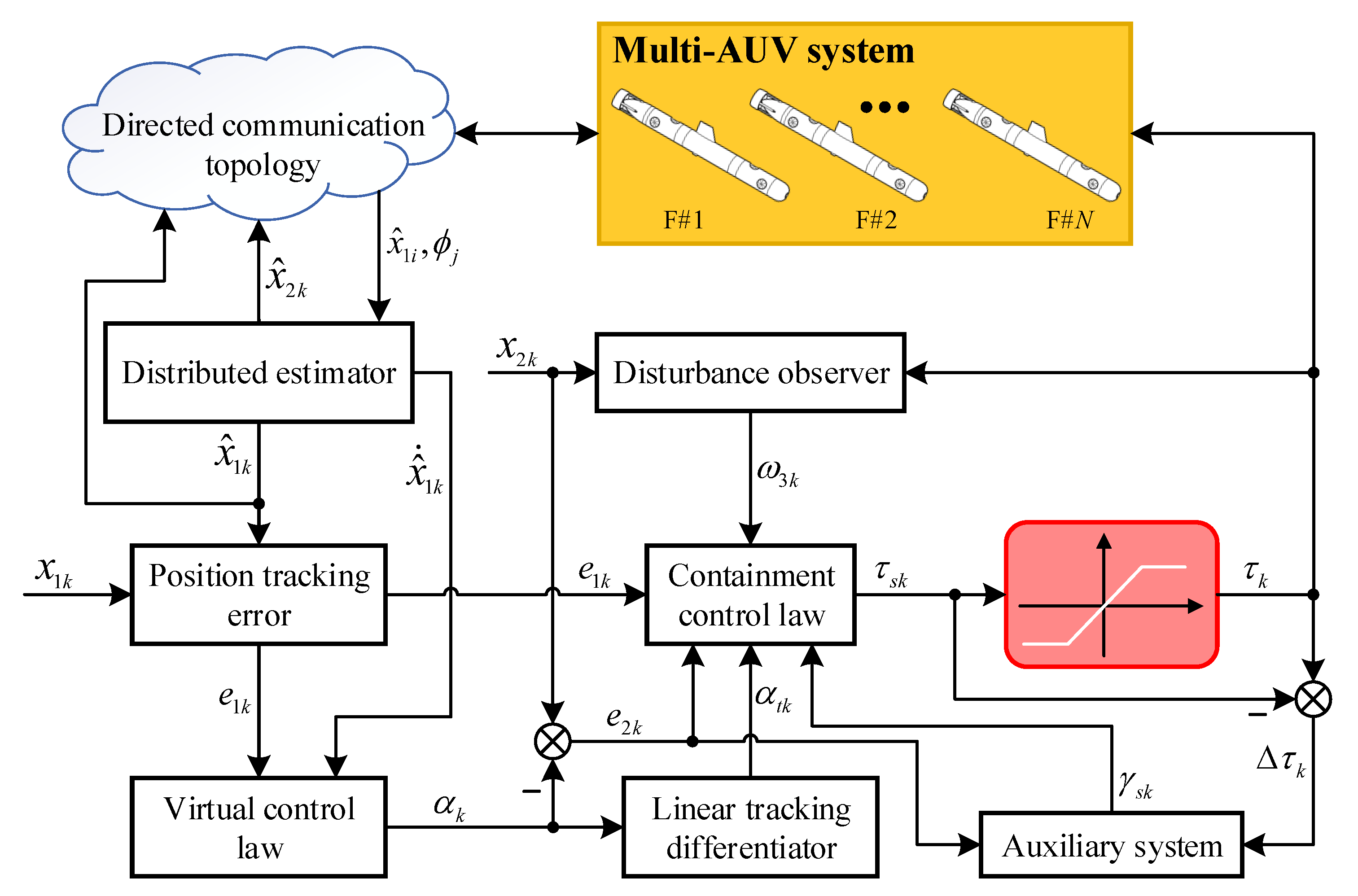
• Due to only a portion of AUVs being able to receive information from virtual leaders, distributed estimators are constructed to acquire accurate estimation information of the follower AUVs’ desired position. Compared with the centralized estimation control algorithm that needs to use a specific AUV to transmit information, the distributed estimation algorithm has a wider application, because each AUV is merely required to acquire its neighbors’ information.
• The control algorithm of this paper is proposed under the condition of directed communication topology. Compared with the control algorithm under an undirected communication topology, the control algorithm designed in this paper does not request two-way communication between AUVs, which is conducive to reducing the burden of communication equipment.
• The internal uncertainties and external disturbances are viewed as composite disturbances, and a disturbance observer is established for estimating and compensating for them, which reduces their adverse effects on the multi-AUV system and improves the system’s anti-disturbance ability. Compared to the method of designing a constant upper bound for disturbance, the conservatism of the algorithm is reduced.
• To address the issue of input saturation, the auxiliary system is constructed to limit the amplitude of control forces and torques, which reduces the unfavorable influence of input saturation on the multi-AUV system, improves the anti-saturation ability of the system, and further strengthens the stability and safety of the system.

The remaining sections of this article are presented below. In Section 2, the basic knowledge of communication topology, the mathematical model of AUVs, and the control objective of this article are introduced in detail. The specific design steps of the containment control scheme are provided in Section 3. The simulation results and conclusions are provided in Section 4 and Section 5, respectively.

Notations: Throughout this article, ${\parallel ·\parallel }_1$, $\parallel ·\parallel$, and ${\parallel ·\parallel }_{\infty }$ signify the 1-norm, 2-norm and ∞-norm of a matrix, respectively. Given a vector $g={[g_1,g_2,\cdots ,g_n]}^T\in {\mathbb{R}}^n$, define ${\mathrm{sig}}^{1/2}\left(g\right)={[\sqrt{|g_1|}\mathrm{sign}\left(g_1\right),\sqrt{|g_2|}\mathrm{sign}\left(g_2\right),\cdots ,\sqrt{|g_n|}\mathrm{sign}\left(g_n\right)]}^T$, in which $\mathrm{sign}(·)$ is the signum function.

2. Preliminaries

2.1. Communication Topology

Take into consideration a multi-AUV system comprised of $\mathcal{N}$ follower AUVs and $\mathcal{M}$ virtual leaders. The sets of follower AUVs and virtual leaders are denoted as $\mathcal{F}=\{1,2,\cdots ,\mathcal{N}\}$ and $\mathcal{L}=\{\mathcal{N}+1,\mathcal{N}+2,\cdots ,\mathcal{N}+\mathcal{M}\}$, respectively. Here, a directed graph $\mathcal{G}(\mathcal{V},\mathcal{E},\mathcal{A})$ is used, describing the communication topology between the virtual leaders and follower AUVs and among the follower AUVs. Here, $\mathcal{V}=\{1,2,\cdots ,\mathcal{N}+\mathcal{M}\}$ represents the node set, $\mathcal{E}=\left\{\right(i,j)\in \mathcal{V}\times \mathcal{V}\}$ denotes the edge set, and $\mathcal{A}={\left[a_{ij}\right]}_{(\mathcal{N}+\mathcal{M})\times (\mathcal{N}+\mathcal{M})}$ signifies the adjacency matrix. The element $a_{ij}$ of $\mathcal{A}$ is depicted as follows:

$$a_{ij}=\left\{\begin{array}{c}\hfill 1,\mathrm{if}(i,j)\in \mathcal{E}\hfill \\ \hfill 0,\mathrm{if}(i,j)\notin \mathcal{E}\hfill \end{array}\right.$$

(1)

where $(i,j)\in \mathcal{E}$ standing for i can receive the information from j. The i’ neighbor set is signified as ${\mathcal{N}}_i=\left\{j\right|(i,j)\in \mathcal{E}\}$. $\mathcal{L}={\left[l_{ij}\right]}_{(\mathcal{N}+\mathcal{M})\times (\mathcal{N}+\mathcal{M})}$ represents the Laplacian matrix, and its element $l_{ij}$ is described as follows:

$$l_{ij}=\left\{\begin{array}{c}\hfill -a_{ij},\mathrm{if}i\ne j\hfill \\ \hfill \sum _{j\in {\mathcal{N}}_i}{a}_{ij},\mathrm{if}i=j\hfill \end{array}\right.$$

(2)

The Laplacian matrix $\mathcal{L}$ is also partitioned as follows:

$$\mathcal{L}=\left[\begin{array}{cc}{0}_{\mathcal{M}\times \mathcal{M}}& 0_{\mathcal{M}\times \mathcal{N}}\\ {\mathcal{L}}_1& {\mathcal{L}}_2\end{array}\right]$$

(3)

where ${\mathcal{L}}_1\in {\mathbb{R}}^{\mathcal{N}\times \mathcal{M}}$ is the sub-matrix that is interrelated to the communication relationship from the virtual leaders to the follower AUVs, and ${\mathcal{L}}_2\in {\mathbb{R}}^{\mathcal{N}\times \mathcal{N}}$ is the sub-matrix that is interrelated to the communication relationship among the follower AUVs. In this paper, we consider that each follower AUV has at least one neighbor, and each virtual leader has no neighbor.

Remark 1. 

The edge set $\mathcal{E}=\left\{\right(i,j)\in \mathcal{V}\times \mathcal{V}\}$ refers to whether there is communication between the AUVs in the system. The node pair $(i,j)$ indicates that AUV i can receive information from AUV j, and AUV j is called a neighbor of AUV i.

Assumption 1. 

For every follower AUV, there is at least one virtual leader that has a directed path to the follower AUV.

Lemma 1 

([38]). Provided that the condition of Assumption 1 is satisfied, each row sum and each entry of ${\mathcal{L}}_2^{-1}{\mathcal{L}}_1$ are equal to 1 and non-negative, respectively, and ${\mathcal{L}}_2\in {\mathbb{R}}^{\mathcal{N}\times \mathcal{N}}$ is a symmetric positive-definite matrix.

2.2. AUV Model

The mathematical model of the k-th follower AUV is given as follows:

$$\left\{\begin{array}{c}{\dot{\eta }}_k=J_k\left({\eta }_k\right){\vartheta }_k\hfill \\ \hfill M_k{\dot{\vartheta }}_k+C_k\left({\vartheta }_k\right){\vartheta }_k+D_k\left({\vartheta }_k\right){\vartheta }_k+g_k\left({\eta }_k\right)={\tau }_k+{\tau }_{dk}\hfill \end{array}\right.$$

(4)

where $k\in \mathcal{F}$. ${\eta }_k={[x_k,y_k,z_k,{\theta }_k,{\psi }_k]}^T$ and ${\vartheta }_k={[u_k,v_k,w_k,q_k,r_k]}^T$ denote the position in the earth-fixed frame and velocity in the body-fixed frame of the AUV, respectively, which are displayed in Figure 1. The transformation matrix $J_k\left({\eta }_k\right)$ is described as follows:

$$J_k\left({\eta }_k\right)=\left[\begin{array}{cc}{J}_{1k}\left({\eta }_k\right)& 0_{3\times 2}\\ 0_{2\times 3}& J_{2k}\left({\eta }_k\right)\end{array}\right]$$

(5)

where

$$\begin{array}{cc}\hfill J_{1k}\left({\eta }_k\right)& \hfill =\left[\begin{array}{ccc}cos\left({\theta }_k\right)cos\left({\psi }_k\right)& -sin\left({\psi }_k\right)& sin\left({\theta }_k\right)cos\left({\psi }_k\right)\\ cos\left({\theta }_k\right)sin\left({\psi }_k\right)& cos\left({\psi }_k\right)& sin\left({\theta }_k\right)sin\left({\psi }_k\right)\\ -sin\left({\theta }_k\right)& 0& cos\left({\theta }_k\right)\end{array}\right]\hfill \\ \hfill J_{2k}\left({\eta }_k\right)& =\left[\begin{array}{cc}1& 0\\ 0& 1/cos\left({\theta }_k\right)\end{array}\right]\hfill \end{array}$$

$M_k$, $C_k\left({\vartheta }_k\right)$, and $D_k\left({\vartheta }_k\right)$ signify the inertia matrix, the Coriolis-centripetal matrix, and the hydrodynamic damping matrix, respectively. $g_k\left({\eta }_k\right)$ stands for the restoring forces and moments. ${\tau }_{dk}$ is the bounded external disturbance. ${\tau }_k={[{\tau }_{uk},{\tau }_{vk},{\tau }_{wk},{\tau }_{qk},{\tau }_{rk}]}^T$ denotes the actual control input. Due to input limitations, the control input should be written as ${\tau }_k=\mathrm{sat}\left({\tau }_{sk}\right)$, with ${\tau }_{sk}$ standing for the command control input and $\mathrm{sat}\left({\tau }_{sk}\right)={[\mathrm{sat}\left({\tau }_{suk}\right),\mathrm{sat}\left({\tau }_{svk}\right),\mathrm{sat}\left({\tau }_{swk}\right),\mathrm{sat}\left({\tau }_{sqk}\right),\mathrm{sat}\left({\tau }_{srk}\right)]}^T$. $\mathrm{sat}(·)$ standing for the saturation function:

$$\mathrm{sat}\left({\tau }_{sik}\right)=\left\{\begin{array}{c}{\tau }_{ik}^{max}\mathrm{sign}\left({\tau }_{sik}\right),\left|{\tau }_{sik}\right|>{\tau }_{ik}^{max}\hfill \\ \hfill {\tau }_{sik},\left|{\tau }_{sik}\right|\le {\tau }_{ik}^{max}\hfill \end{array}\right.$$

(6)

where $i=u,v,w,q,r$. ${\tau }_k^{max}={[{\tau }_{uk}^{max},{\tau }_{vk}^{max},{\tau }_{wk}^{max},{\tau }_{qk}^{max},{\tau }_{rk}^{max}]}^T$ signifies the maximum forces and moments.

Next, we transform the model of the k-th follower AUV into the following form:

$$\left\{\begin{array}{cc}\hfill {\dot{x}}_{1k}& =x_{2k}\hfill \\ \hfill {\dot{x}}_{2k}& =Q_k({\vartheta }_k,{\eta }_k)+B_k{\tau }_k\hfill \\ \hfill {\eta }_k& =x_{1k}\hfill \end{array}\right.$$

(7)

where

$$\begin{array}{cc}\hfill & x_{2k}={\dot{\eta }}_k,{\overline{M}}_k\left({\eta }_k\right)=M_k{J}^{-1}\left({\eta }_k\right),B_k={\overline{M}}_k{\left({\eta }_k\right)}^{-1}\hfill \\ \hfill & {\overline{C}}_k\left({\eta }_k\right)=[C_k\left({\vartheta }_k\right)+D_k\left({\vartheta }_k\right)-M_k{J}^{-1}\left({\eta }_k\right)\dot{J}\left({\eta }_k\right)]J^{-1}\left({\eta }_k\right)\hfill \\ \hfill & Q_k({\vartheta }_k,{\eta }_k)=-{\overline{M}}_k{\left({\eta }_k\right)}^{-1}{\overline{C}}_k\left({\eta }_k\right){\dot{\eta }}_k-{\overline{M}}_k{\left({\eta }_k\right)}^{-1}{g}_k\left({\eta }_k\right)+{\overline{M}}_k{\left({\eta }_k\right)}^{-1}{\tau }_{dk}\hfill \end{array}$$

with $Q_k({\vartheta }_k,{\eta }_k)$ representing the composite disturbance of the k-th follower AUV, which contains the internal model uncertainties and external bounded disturbances.

Assumption 2. 

The elements of $Q_k({\vartheta }_k,{\eta }_k)$ and its time derivative are bounded. In other words, there exists a constant $C_d\ge 0$ such that $\parallel {\dot{Q}}_k({\vartheta }_k,{\eta }_k)\parallel \le C_d$.

2.3. Control Objective

Our research objective is to develop a distributed estimator-based containment controller for multi-AUV systems such that the following formula is satisfied:

$$\underset{t\to \infty }{lim}\parallel x_{1k}-\sum _{i=\mathcal{N}+1}^{\mathcal{N}+\mathcal{M}}{\hslash }_{ik}{\varphi }_i\parallel \le \zeta ,k=1,2,\cdots ,\mathcal{N}$$

(8)

namely, each follower AUV in a multi-AUV system can enter into a convex hull that is formed by the virtual leaders. $\zeta \in \mathbb{R}$ is a small positive constant. ${\varphi }_i(i\in \mathcal{L})$ signifies the position vector of the virtual leader i. ${\hslash }_{ik}\in \mathbb{R}$ satisfies ${\sum }_{i=\mathcal{N}+1}^{\mathcal{N}+\mathcal{M}}{\hslash }_{ik}=1$ and ${\hslash }_{ik}\ge 0$.

Assumption 3. 

The second-order derivative of the position vectors for the virtual leaders is bounded; that is, $\parallel {\ddot{\varphi }}_i\parallel \le \mu$ $(i\in \mathcal{L})$, with μ being a positive scalar.

3. Containment Control Scheme Design

In this section, the major goal is to design a containment control scheme for the multi-AUV system such that the control objective in Section 2.3 can be achieved. The structure diagram of the containment control scheme for the multi-AUV system is displayed in Figure 2.

3.1. Distributed Estimator Design

Motivated by [38], the distributed estimator for the k-th follower AUV is put forward as follows:

$$\left\{\begin{array}{cc}\hfill {\dot{\widehat{x}}}_{1k}& \hfill ={\widehat{x}}_{2k}-{\delta }_1\mathrm{sign}\left(\sum _{i=1}^{\mathcal{N}}{a}_{ki}({\widehat{x}}_{1k}-{\widehat{x}}_{1i})+\sum _{j=\mathcal{N}+1}^{\mathcal{N}+\mathcal{M}}{a}_{kj}({\widehat{x}}_{1k}-{\varphi }_j)\right)\hfill \\ \hfill {\dot{\widehat{x}}}_{2k}& \hfill =-{\delta }_2\mathrm{sign}\left(\sum _{i=1}^{\mathcal{N}}{a}_{ki}({\widehat{x}}_{2k}-{\widehat{x}}_{2i})+\sum _{j=\mathcal{N}+1}^{\mathcal{N}+\mathcal{M}}{a}_{kj}({\widehat{x}}_{2k}-{\dot{\varphi }}_j)\right)\hfill \end{array}\right.$$

(9)

where $k\in \mathcal{F}$. ${\delta }_1$ and ${\delta }_2$ are given positive scalars. ${\widehat{x}}_{1k}$ and ${\widehat{x}}_{2k}$ denote the estimators of ${\eta }_{dk}$ and ${\dot{\eta }}_{dk}$, respectively, in which ${\eta }_{dk}$ is the weighed average of the virtual leaders’ position. In other words, ${\eta }_{dk}$ is the reference position of the k-th follower AUV.

For the convenience of the following statements, let $x_{1\mathcal{F}}={[x_{11}^T,x_{12}^T,\cdots ,x_{1\mathcal{N}}^T]}^T$, ${\varphi }_{\mathcal{L}}={[{\varphi }_{\mathcal{N}+1}^T,{\varphi }_{\mathcal{N}+2}^T,\cdots ,{\varphi }_{\mathcal{N}+\mathcal{M}}^T]}^T$, ${\widehat{x}}_{1\mathcal{F}}={[{\widehat{x}}_{11}^T,{\widehat{x}}_{12}^T,\cdots ,{\widehat{x}}_{1\mathcal{N}}^T]}^T$ and ${\widehat{x}}_{2\mathcal{F}}={[{\widehat{x}}_{21}^T,{\widehat{x}}_{22}^T,\cdots ,{\widehat{x}}_{2\mathcal{N}}^T]}^T$. Define ${\eta }_{d\mathcal{F}}={[{\eta }_{d1}^T,{\eta }_{d2}^T,\cdots ,{\eta }_{d\mathcal{N}}^T]}^T=-({\mathcal{L}}_2^{-1}{\mathcal{L}}_1\otimes I_5){\varphi }_{\mathcal{L}}$ as the set of the follower AUVs’ desired position. According to Lemma 1 and Section 2.3, we can know that ${\eta }_{d\mathcal{F}}$ is always within the convex hull formed by the virtual leaders. Hence, the control objective of the follower AUVs is achieved if $x_{1\mathcal{F}}={\eta }_{d\mathcal{F}}$. Next, for the designed distributed estimator (9), the following theorem is given.

Theorem 1. 

Let ${\delta }_1>0$ and ${\delta }_2>\mu$. If the conditions of Assumptions 1–3 hold, under the action of the designed distributed estimator (9), ${\widehat{x}}_{1\mathcal{F}}$ and ${\widehat{x}}_{2\mathcal{F}}$ can converge asymptotically to ${\eta }_{d\mathcal{F}}$ and ${\dot{\eta }}_{d\mathcal{F}}$.

Proof.  

Let ${\tilde{x}}_{1\mathcal{F}}={\widehat{x}}_{1\mathcal{F}}-{\eta }_{d\mathcal{F}}={\widehat{x}}_{1\mathcal{F}}+({\mathcal{L}}_2^{-1}{\mathcal{L}}_1\otimes I_5){\varphi }_{\mathcal{L}}$ and ${\tilde{x}}_{2\mathcal{F}}={\widehat{x}}_{2\mathcal{F}}-{\dot{\eta }}_{d\mathcal{F}}={\widehat{x}}_{2\mathcal{F}}+({\mathcal{L}}_2^{-1}{\mathcal{L}}_1\otimes I_5){\dot{\varphi }}_{\mathcal{L}}$. Based on the distributed estimator (9), the Lyapunov function is constructed as follows:

$$V_1={\displaystyle \frac{1}{2}}{\tilde{x}}_{2\mathcal{F}}^T{({\mathcal{L}}_2\otimes I_5)}^T{\tilde{x}}_{2\mathcal{F}}$$

(10)

Taking the derivative of $V_1$, one yields the following:

$$\begin{array}{cc}\hfill {\dot{V}}_1& ={\tilde{x}}_{2\mathcal{F}}^T{({\mathcal{L}}_2\otimes I_5)}^T{\dot{\tilde{x}}}_{2\mathcal{F}}\hfill \\ \hfill & ={\tilde{x}}_{2\mathcal{F}}^T{({\mathcal{L}}_2\otimes I_5)}^T[{\dot{\widehat{x}}}_{2\mathcal{F}}+({\mathcal{L}}_2^{-1}{\mathcal{L}}_1\otimes I_5){\ddot{\varphi }}_{\mathcal{L}}]\hfill \\ \hfill & ={\left(({\mathcal{L}}_2\otimes I_5){\tilde{x}}_{2\mathcal{F}}\right)}^T[-{\delta }_2\mathrm{sign}\left(({\mathcal{L}}_2\otimes I_5){\tilde{x}}_{2\mathcal{F}}\right)+({\mathcal{L}}_2^{-1}{\mathcal{L}}_1\otimes I_5){\ddot{\varphi }}_{\mathcal{L}}]\hfill \\ \hfill & =-{\delta }_2{\parallel ({\mathcal{L}}_2\otimes I_5){\tilde{x}}_{2\mathcal{F}}\parallel }_1+{\left(({\mathcal{L}}_2\otimes I_5){\tilde{x}}_{2\mathcal{F}}\right)}^T({\mathcal{L}}_2^{-1}{\mathcal{L}}_1\otimes I_5){\ddot{\varphi }}_{\mathcal{L}}\hfill \end{array}$$

(11)

According to [39], for any matrix $A\in {\mathbb{R}}^{m\times n}$, one obtains the following:

$$\parallel A\parallel \le \sqrt{m}{\parallel A\parallel }_{\infty }$$

(12)

$${\displaystyle \frac{1}{\sqrt{m}}}{\parallel A\parallel }_1\le \parallel A\parallel \le \sqrt{n}{\parallel A\parallel }_1$$

(13)

In view of Assumption 3, Lemma 1, (12), and (13), one obtains the following:

$$\begin{array}{cc}\hfill {\dot{V}}_1& \le -{\delta }_2\parallel ({\mathcal{L}}_2\otimes I_5){\tilde{x}}_{2\mathcal{F}}{\parallel }_1+\parallel {\left(({\mathcal{L}}_2\otimes I_5){\tilde{x}}_{2\mathcal{F}}\right)}^T({\mathcal{L}}_2^{-1}{\mathcal{L}}_1\otimes I_5){\ddot{\varphi }}_{\mathcal{L}}\parallel \hfill \\ \hfill & \le -{\delta }_2\parallel ({\mathcal{L}}_2\otimes I_5){\tilde{x}}_{2\mathcal{F}}{\parallel }_1+\mu \parallel {\mathcal{L}}_2^{-1}{\mathcal{L}}_1\otimes I_5{\parallel }_{\infty }\parallel ({\mathcal{L}}_2\otimes I_5){\tilde{x}}_{2\mathcal{F}}\parallel \hfill \\ \hfill & \le -({\delta }_2-\mu )\parallel ({\mathcal{L}}_2\otimes I_5){\tilde{x}}_{2\mathcal{F}}\parallel \hfill \end{array}$$

(14)

Owing to ${\delta }_2>\mu$, the following can be obtained:

$${\dot{V}}_1<0$$

(15)

Due to $V_1\ge 0$ and ${\dot{V}}_1<0$, we can determine that ${\tilde{x}}_{2\mathcal{F}}$ is asymptotically stable; that is, ${lim}_{t\to \infty }{\tilde{x}}_{2\mathcal{F}}={lim}_{t\to \infty }({\widehat{x}}_{2\mathcal{F}}-{\dot{\eta }}_{d\mathcal{F}})=0$, which means that ${\widehat{x}}_{2\mathcal{F}}$ can converge asymptotically to ${\dot{\eta }}_{d\mathcal{F}}$.

When ${\tilde{x}}_{2\mathcal{F}}$ is asymptotically stable, the following Lyapunov function is constructed:

$$V_2={\displaystyle \frac{1}{2}}{\tilde{x}}_{1\mathcal{F}}^T{({\mathcal{L}}_2\otimes I_5)}^T{\tilde{x}}_{1\mathcal{F}}$$

(16)

Taking the derivative of $V_2$, one obtains the following:

$$\begin{array}{cc}\hfill {\dot{V}}_2& ={\tilde{x}}_{1\mathcal{F}}^T{({\mathcal{L}}_2\otimes I_5)}^T{\dot{\tilde{x}}}_{1\mathcal{F}}\hfill \\ \hfill & ={\tilde{x}}_{1\mathcal{F}}^T{({\mathcal{L}}_2\otimes I_5)}^T[-{\delta }_1\mathrm{sign}\left(({\mathcal{L}}_2\otimes I_5){\tilde{x}}_{1\mathcal{F}}\right)]\hfill \\ \hfill & \le -{\delta }_1{\parallel ({\mathcal{L}}_2\otimes I_5){\tilde{x}}_{1\mathcal{F}}\parallel }_1\hfill \end{array}$$

(17)

Because of ${\delta }_1>0$, the following can be obtained:

$${\dot{V}}_2<0$$

(18)

Owing to $V_2\ge 0$ and ${\dot{V}}_2<0$, it can be determined that ${\tilde{x}}_{1\mathcal{F}}$ is asymptotically stable; namely, ${lim}_{t\to \infty }{\tilde{x}}_{1\mathcal{F}}={lim}_{t\to \infty }({\widehat{x}}_{1\mathcal{F}}-{\eta }_{d\mathcal{F}})=0$, which means that ${\widehat{x}}_{1\mathcal{F}}$ can converge asymptotically to ${\eta }_{d\mathcal{F}}$. □

3.2. Containment Controller Design

In this section, the containment controller of the k-th $(k\in \mathcal{F})$ follower AUV is designed. The detailed steps for designing the containment controller are provided as follows:

Step 1 (Virtual control law design): Define the position tracking error of the k-th follower AUV as follows:

$$e_{1k}=x_{1k}-{\widehat{x}}_{1k}$$

(19)

On the basis of (7), taking the derivative of (19), one obtains the following:

$${\dot{e}}_{1k}=x_{2k}-{\dot{\widehat{x}}}_{1k}$$

(20)

For stabilizing (20), the virtual control law is constructed as follows:

$${\alpha }_k=-H_{1k}{e}_{1k}+{\dot{\widehat{x}}}_{1k}$$

(21)

with $H_{1k}$ being the gain matrix and satisfying $H_{1k}=H_{1k}^T>0$. Substituting (21) into (20), one obtains the following:

$${\dot{e}}_{1k}=x_{2k}-{\alpha }_k-H_{1k}{e}_{1k}=e_{2k}-H_{1k}{e}_{1k}$$

(22)

with $e_{2k}=x_{2k}-{\alpha }_k$.

Step 2 (Containment control law design): Taking the derivative of $e_{2k}$, the following can be obtained:

$${\dot{e}}_{2k}={\dot{x}}_{2k}-{\dot{\alpha }}_k=Q_k({\vartheta }_k,{\eta }_k)+B_k{\tau }_k-{\dot{\alpha }}_k$$

(23)

For acquiring the derivative information of ${\alpha }_k$, we introduce the linear tracking differentiator as follows:

$$\left\{\begin{array}{cc}\hfill {\dot{\alpha }}_{dk}& ={\alpha }_{tk}\hfill \\ \hfill {\dot{\alpha }}_{tk}& =-{ϵ}_{dk}^2({\alpha }_{dk}-{\alpha }_k)-2{ϵ}_{dk}{\alpha }_{tk}\hfill \end{array}\right.$$

(24)

with ${\alpha }_{tk}$ being the estimated value of $\dot{{\alpha }_k}$ and ${ϵ}_{dk}$ being a positive constant. Based on the convergence analysis of the linear tracking differentiator in [40], we can determine that there exist two small constants, $h_c$ and $h_d$, satisfying the following:

$$\parallel {\alpha }_{dk}-{\alpha }_k\parallel \le h_c,\parallel {\alpha }_{tk}-{\dot{\alpha }}_k\parallel \le h_s$$

(25)

For the sake of estimating the composite disturbance $Q_k({\vartheta }_k,{\eta }_k)$ in (7), the disturbance observer is taken as follows:

$$\left\{\begin{array}{cc}\hfill {\dot{\omega }}_{1k}& ={\omega }_{2k}+B_k{\tau }_k\hfill \\ \hfill {\omega }_{2k}& =-{\beta }_1{C}^{1/2}{\mathrm{sig}}^{1/2}({\omega }_{1k}-x_{2k})+{\omega }_{3k}\hfill \\ \hfill {\dot{\omega }}_{3k}& =-{\beta }_{2}C\mathrm{sign}({\omega }_{3k}-{\omega }_{2k})\hfill \end{array}\right.$$

(26)

with ${\omega }_{3k}$ being the estimated value of $Q_k({\vartheta }_k,{\eta }_k)$, ${\beta }_1>0$ and ${\beta }_2>0$ being the given constants, and $C=\mathrm{diag}\{c_1,c_2,c_3,c_4,c_5\}$ being the positive definite diagonal matrix. Then, the following theorem is provided for the designed disturbance observer (26).

Theorem 2. 

The composite disturbance $Q_k({\vartheta }_k,{\eta }_k)$ can be exactly observed by utilizing the designed disturbance observer (26) within a short time.

Proof.  

The error variables are defined as follows:

$$q_{1k}={\omega }_{1k}-x_{2k}$$

(27)

$$q_{2k}={\omega }_{3k}-Q_k({\vartheta }_k,{\eta }_k)$$

(28)

Based on (26), the derivatives of $q_{1k}$ and $q_{2k}$ are easily obtained as follows:

$$\begin{array}{cc}\hfill {\dot{q}}_{1k}& ={\dot{\omega }}_{1k}-{\dot{x}}_{2k}\hfill \\ \hfill & =-{\beta }_1{C}^{1/2}{\mathrm{sig}}^{1/2}({\omega }_{1k}-x_{2k})+{\omega }_{3k}-Q_k({\vartheta }_k,{\eta }_k)\hfill \\ \hfill & =-{\beta }_1{C}^{1/2}{\mathrm{sig}}^{1/2}\left(q_{1k}\right)+q_{2k}\hfill \end{array}$$

(29)

$$\begin{array}{cc}\hfill {\dot{q}}_{2k}& ={\dot{\omega }}_{3k}-{\dot{Q}}_k({\vartheta }_k,{\eta }_k)\hfill \\ \hfill & =-{\beta }_{2}C\mathrm{sign}({\omega }_{3k}-{\omega }_{2k})-{\dot{Q}}_k({\vartheta }_k,{\eta }_k)\hfill \\ \hfill & =-{\beta }_{2}C\mathrm{sign}(q_{2k}-{\dot{q}}_{1k})-{\dot{Q}}_k({\vartheta }_k,{\eta }_k)\hfill \end{array}$$

(30)

In view of Assumption 2, (29), and (30), it can be determined that the elements of ${\dot{q}}_{1k}$ and ${\dot{q}}_{2k}$ satisfy the following:

$${\dot{q}}_{1kj}=-{\beta }_1{c}_j^{1/2}{\mathrm{sig}}^{1/2}\left(q_{1kj}\right)+q_{2kj}$$

(31)

$${\dot{q}}_{2kj}=-{\beta }_2{c}_j\mathrm{sign}(q_{2kj}-{\dot{q}}_{1kj})+[-C_d,C_d]$$

(32)

where $q_{1kj}$, $q_{2kj}$ and $c_j$ $(j=1,2,\cdots ,5)$ denote the elements of $q_{1k}$, $q_{2k}$ and C, respectively. According to [41], it follows that the error variables $q_{1k}$ and $q_{2k}$ are stable in finite time. That is to say, for a short time $T>0$, the following equalities hold:

$${\omega }_{1k}\equiv x_{2k},{\omega }_{3k}\equiv Q_k({\vartheta }_k,{\eta }_k),\forall t>T$$

(33)

□

Based on the contents of Section 2.2, one determines that ${\tau }_k=\mathrm{sat}\left({\tau }_{sk}\right)$, with ${\tau }_{sk}$ being the command control input; i.e., the containment control law to be designed. For stabilizing (23), ${\tau }_{sk}$ is designed in the following form:

$${\tau }_{sk}=B_k^{-1}(-H_{2k}{e}_{2k}-e_{1k}-{\omega }_{3k}+{\alpha }_{tk}+H_{3k}{\gamma }_{sk})$$

(34)

where $H_{2k}$ and $H_{3k}$ are the gain matrices satisfying $H_{2k}=H_{2k}^T>0$, and $H_{3k}=H_{3k}^T>0$. ${\gamma }_{sk}$ is the state variable in (35). To tackle the issue of input saturation, an auxiliary system is constructed:

$${\dot{\gamma }}_{sk}=\left\{\begin{array}{c}-H_{4k}{\gamma }_{sk}-{\left({\gamma }_{sk}^T\right)}^{+}\left(|e_{2k}^T{B}_k\Delta {\tau }_k|+{\displaystyle \frac{1}{2}}\Delta {\tau }_k^T\Delta {\tau }_k\right)+\Delta {\tau }_k,\parallel {\gamma }_{sk}\parallel \ge b\hfill \\ 0_{5\times 1},\parallel {\gamma }_{sk}\parallel <b\hfill \end{array}\right.$$

(35)

where $\Delta {\tau }_k={\tau }_k-{\tau }_{sk}$, $H_{4k}$ is a gain matrix satisfying $H_{4k}=H_{4k}^T>0$ and b is a positive constant. ${\left({\gamma }_{sk}^T\right)}^{+}$ denotes the Moore–Penrose inverse of ${\gamma }_{sk}^T$. Incorporating (24)–(35) into (23), one yields the following:

$${\dot{e}}_{2k}=-H_{2k}{e}_{2k}-e_{1k}+({\alpha }_{tk}-{\dot{\alpha }}_k)+H_{3k}{\gamma }_{sk}+B_k\Delta {\tau }_k$$

(36)

3.3. Stability Analysis

Theorem 3. 

Considering a group of AUVs described by (4), under Assumptions 1–3, the containment control of the multi-AUV system can be achieved with the assistance of the distributed estimator (9), the virtual control law (21), the linear tracking differentiator (24), the disturbance observer (26), the containment control law (34), and the auxiliary system (35). In the meantime, the containment errors of the multi-AUV system are uniformly ultimately bounded.

Proof.  

Consider the below Lyapunov function:

$$V_3=\sum _{k=1}^{\mathcal{N}}\left({\displaystyle \frac{1}{2}}{e}_{1k}^T{e}_{1k}+{\displaystyle \frac{1}{2}}{e}_{2k}^T{e}_{2k}+{\displaystyle \frac{1}{2}}{\gamma }_{sk}^T{\gamma }_{sk}\right)$$

(37)

Taking the derivative of the above formula (37), one obtains the following:

$${\dot{V}}_3=\sum _{k=1}^{\mathcal{N}}\left(e_{1k}^T{\dot{e}}_{1k}+e_{2k}^T{\dot{e}}_{2k}+{\gamma }_{sk}^T{\dot{\gamma }}_{sk}\right)$$

(38)

On the basis of (22), (25), and (36), and employing Young’s inequality, one obtains the following:

$$\begin{array}{cc}\hfill & e_{1k}^T{\dot{e}}_{1k}+e_{2k}^T{\dot{e}}_{2k}\hfill \\ \hfill =& e_{1k}^T(e_{2k}-H_{1k}{e}_{1k})+e_{2k}^T(-H_{2k}{e}_{2k}-e_{1k}+({\alpha }_{tk}-{\dot{\alpha }}_k)+H_{3k}{\gamma }_{sk}+B_k\Delta {\tau }_k)\hfill \\ \hfill =& -e_{1k}^T{H}_{1k}{e}_{1k}-e_{2k}^T{H}_{2k}{e}_{2k}+e_{2k}^T({\alpha }_{tk}-{\dot{\alpha }}_k)+e_{2k}^T{H}_{3k}{\gamma }_{sk}+e_{2k}^T{B}_k\Delta {\tau }_k\hfill \\ \hfill \le & -e_{1k}^T{H}_{1k}{e}_{1k}-e_{2k}^T{H}_{2k}{e}_{2k}+e_{2k}^T{e}_{2k}+{\displaystyle \frac{1}{2}}{({\alpha }_{tk}-{\dot{\alpha }}_k)}^T({\alpha }_{tk}-{\dot{\alpha }}_k)\hfill \\ \hfill & +{\displaystyle \frac{1}{2}}{\gamma }_{sk}^T{H}_{3k}^T{H}_{3k}{\gamma }_{sk}+e_{2k}^T{B}_k\Delta {\tau }_k\hfill \\ \hfill \le & -{\lambda }_{min}\left(H_{1k}\right)\parallel e_{1k}{\parallel }^2-[{\lambda }_{min}\left(H_{2k}\right)-1]\parallel e_{2k}{\parallel }^2+{\displaystyle \frac{1}{2}}{h}_s^2+{\displaystyle \frac{1}{2}}\parallel H_{3k}{\parallel }^2{\parallel {\gamma }_{sk}\parallel }^2+e_{2k}^T{B}_k\Delta {\tau }_k\hfill \end{array}$$

(39)

with ${\lambda }_{min}(·)$ standing for the minimum eigenvalue of a matrix.

Subsequently, two situations, i.e., $\parallel {\gamma }_{sk}\parallel \ge b$ and $\parallel {\gamma }_{sk}\parallel <b$, need to be taken into account to discuss the stability of the multi-AUV system.

Situation 1: $\parallel {\gamma }_{sk}\parallel \ge b$. According to (35), one obtains the following:

$${\gamma }_{sk}^T{\dot{\gamma }}_{sk}=-{\gamma }_{sk}^T{H}_{4k}{\gamma }_{sk}-|e_{2k}^T{B}_k\Delta {\tau }_k|-{\displaystyle \frac{1}{2}}\Delta {\tau }_k^T\Delta {\tau }_k-{\gamma }_{sk}^T\Delta {\tau }_k$$

(40)

With the help of Young’s inequality, one can obtain the following:

$$-{\gamma }_{sk}^T\Delta {\tau }_k\le {\displaystyle \frac{1}{2}}{\gamma }_{sk}^T{\gamma }_{sk}+{\displaystyle \frac{1}{2}}\Delta {\tau }_k^T\Delta {\tau }_k$$

(41)

Substituting (41) into (40), one obtains the following:

$$\begin{array}{cc}\hfill {\gamma }_{sk}^T{\dot{\gamma }}_{sk}& \le -{\gamma }_{sk}^T{H}_{4k}{\gamma }_{sk}-|e_{2k}^T{B}_k\Delta {\tau }_k|+{\displaystyle \frac{1}{2}}{\gamma }_{sk}^T{\gamma }_{sk}\hfill \\ \hfill & \le -\left[{\lambda }_{min}\left(H_{4k}\right)-{\displaystyle \frac{1}{2}}\right]\parallel {\gamma }_{sk}{\parallel }^2-|e_{2k}^T{B}_k\Delta {\tau }_k|\hfill \end{array}$$

(42)

Incorporating (39) and (42) into (38), one yields the following:

$$\begin{array}{cc}\hfill {\dot{V}}_3\le & \sum _{k=1}^{\mathcal{N}}(-{\lambda }_{min}\left(H_{1k}\right)\parallel e_{1k}{\parallel }^2-[{\lambda }_{min}\left(H_{2k}\right)-1]{\parallel e_{2k}\parallel }^2\hfill \\ \hfill & -\left[{\lambda }_{min}\left(H_{4k}\right)-{\displaystyle \frac{1}{2}}{\parallel H_{3k}\parallel }^2-{\displaystyle \frac{1}{2}}\right]{\parallel {\gamma }_{sk}\parallel }^2+{\displaystyle \frac{1}{2}}{h}_s^2)\hfill \end{array}$$

(43)

Denote ${\kappa }_1={min}_{k\in \mathcal{F}}\{{\lambda }_{min}\left(H_{1k}\right),{\lambda }_{min}\left(H_{2k}\right)-1,{\lambda }_{min}\left(H_{4k}\right)-{\displaystyle \frac{1}{2}}\parallel H_{3k}{\parallel }^2-{\displaystyle \frac{1}{2}}\}$ and ${\mathsf{\Phi }}_1={\displaystyle \frac{1}{2}}{\sum }_{k=1}^{\mathcal{N}}{h}_s^2$. Therefore, (43) can be further written as follows:

$${\dot{V}}_3\le -2{\kappa }_1{V}_3+{\mathsf{\Phi }}_1$$

(44)

Situation 2: $\parallel {\gamma }_{sk}\parallel <b$. On the basis of (35), one has the following:

$${\gamma }_{sk}^T{\dot{\gamma }}_{sk}=0$$

(45)

On account of Young’s inequality, the following can be determined:

$$\begin{array}{cc}\hfill {\displaystyle \frac{1}{2}}\parallel H_{3k}{\parallel }^2{\parallel {\gamma }_{sk}\parallel }^2& =-{\displaystyle \frac{1}{2}}\parallel H_{3k}{\parallel }^2\parallel {\gamma }_{sk}{\parallel }^2+\parallel H_{3k}{\parallel }^2{\parallel {\gamma }_{sk}\parallel }^2\hfill \\ \hfill & \le -{\displaystyle \frac{1}{2}}\parallel H_{3k}{\parallel }^2\parallel {\gamma }_{sk}{\parallel }^2+{\parallel H_{3k}\parallel }^2{b}^2\hfill \end{array}$$

(46)

$$e_{2k}^T{B}_k\Delta {\tau }_k\le {\displaystyle \frac{1}{2}}\parallel e_{2k}{\parallel }^2+{\displaystyle \frac{1}{2}}{\parallel B_k\Delta {\tau }_k\parallel }^2$$

(47)

Incorporating (39), (46), and (47) into (38), one obtains the following:

$$\begin{array}{cc}\hfill {\dot{V}}_3\le & \sum _{k=1}^{\mathcal{N}}(-{\lambda }_{min}\left(H_{1k}\right)\parallel e_{1k}{\parallel }^2-\left[{\lambda }_{min}\left(H_{2k}\right)-{\displaystyle \frac{3}{2}}\right]{\parallel e_{2k}\parallel }^2\hfill \\ \hfill & -{\displaystyle \frac{1}{2}}\parallel H_{3k}{\parallel }^2\parallel {\gamma }_{sk}{\parallel }^2+{\displaystyle \frac{1}{2}}{h}_s^2+\parallel H_{3k}{\parallel }^2{b}^2+{\displaystyle \frac{1}{2}}{\parallel B_k\Delta {\tau }_k\parallel }^2)\hfill \end{array}$$

(48)

${\kappa }_2={min}_{k\in \mathcal{F}}\{{\lambda }_{min}\left(H_{1k}\right),{\lambda }_{min}\left(H_{2k}\right)-3/2,\parallel H_{3k}{\parallel }^2/2\parallel \}$ and ${\mathsf{\Phi }}_2={\sum }_{k=1}^{\mathcal{N}}(h_s^2/2+{\parallel H_{3k}\parallel }^2$$b^2+\parallel B_k\Delta {\tau }_k{\parallel }^2/2)$ are denoted. Hence, (48) can be further depicted as follows:

$${\dot{V}}_3\le -2{\kappa }_2{V}_3+{\mathsf{\Phi }}_2$$

(49)

Synthesizing situation 1 and situation 2, one obtains the following:

$${\dot{V}}_3\le -2\kappa V_3+\mathsf{\Phi }$$

(50)

with $\kappa =min\{{\kappa }_1,{\kappa }_2\}$ and $\mathsf{\Phi }=max{\mathsf{\Phi }}_1,{\mathsf{\Phi }}_2$. The designed parameters satisfy ${\lambda }_{min}\left(H_{1k}\right)>0$, ${\lambda }_{min}\left(H_{2k}\right)>3/2$, ${\lambda }_{min}\left(H_{3k}\right)>0$, ${\lambda }_{min}\left(H_{4k}\right)>{\displaystyle \frac{1}{2}}{\parallel H_{3k}\parallel }^2+1/2$.

By solving inequality (50), one yields the following:

$$0\le V_3\le {\displaystyle \frac{\mathsf{\Phi }}{2\kappa }}+\left[V_3\left(0\right)-{\displaystyle \frac{\mathsf{\Phi }}{2\kappa }}\right]e^{-2\kappa t}$$

(51)

which implies that the Lyapunov function $V_3$ is uniformly ultimately bounded. It can be obtained from (37) and (51) that $e_{1k}$, $e_{2k}$ and ${\gamma }_{sk}$ $(k\in \mathcal{F})$ are also uniformly ultimately bounded.

In light of (37) and (51), one has the following:

$$\parallel E_1\parallel =\parallel x_{1\mathcal{F}}-{\widehat{x}}_{1\mathcal{F}}\parallel \le \sqrt{2V_3}\le \sqrt{{\displaystyle \frac{\mathsf{\Phi }}{\kappa }}+\left[2V_3\left(0\right)-{\displaystyle \frac{\mathsf{\Phi }}{\kappa }}\right]e^{-2\kappa t}}$$

(52)

with $E_1={[e_{11}^T,e_{12}^T,\cdots ,e_{1\mathcal{N}}^T]}^T$. From (52), the following can be further obtained:

$$x_{1\mathcal{F}j}-{\widehat{x}}_{1\mathcal{F}j}\le \sqrt{{\displaystyle \frac{\mathsf{\Phi }}{\kappa }}+\left[2V_3\left(0\right)-{\displaystyle \frac{\mathsf{\Phi }}{\kappa }}\right]e^{-2\kappa t}}$$

(53)

where $1_{5\mathcal{N}}={[1,\cdots ,1]}^T\in {\mathbb{R}}^{5\mathcal{N}}$. $x_{1\mathcal{F}j}$ and ${\widehat{x}}_{1\mathcal{F}j}$ $(j=1,2,\cdots ,5\mathcal{N})$ are the elements of $x_{1\mathcal{F}}$ and $x_{1\mathcal{F}}$, respectively. Taking the limit on the above formula (53), one obtains the following:

$$\underset{t\to \infty }{lim}(x_{1\mathcal{F}j}-{\widehat{x}}_{1\mathcal{F}j})\le \sqrt{{\displaystyle \frac{\mathsf{\Phi }}{\kappa }}}$$

(54)

According to Theorem 1, we can determine that ${lim}_{t\to \infty }({\widehat{x}}_{1\mathcal{F}}-{\eta }_{d\mathcal{F}})=0$ under the action of the designed distributed estimator (9), where ${\eta }_{d\mathcal{F}}=-({\mathcal{L}}_2^{-1}{\mathcal{L}}_1\otimes I_5){\varphi }_{\mathcal{L}}$ is the desired position information of the follower AUVs. Based on ${lim}_{t\to \infty }({\widehat{x}}_{1\mathcal{F}}-{\eta }_{d\mathcal{F}})=0$, one has the following:

$$\underset{t\to \infty }{lim}({\widehat{x}}_{1\mathcal{F}j}-{\eta }_{d\mathcal{F}j})=0$$

(55)

where ${\eta }_{d\mathcal{F}j}$ $(j=1,2,\cdots ,5\mathcal{N})$ is the the element of ${\eta }_{d\mathcal{F}}$. Combining (54) and (55), one obtains the following:

$$\underset{t\to \infty }{lim}(x_{1\mathcal{F}j}-{\eta }_{d\mathcal{F}j})\le \sqrt{{\displaystyle \frac{\mathsf{\Phi }}{\kappa }}}$$

(56)

According to Formula (56) above, one yields the following:

$$\underset{t\to \infty }{lim}\parallel x_{1\mathcal{F}}-{\eta }_{d\mathcal{F}}\parallel \le \zeta$$

(57)

where $\varpi ={[\sqrt{\mathsf{\Phi }/\kappa },\cdots ,\sqrt{\mathsf{\Phi }/\kappa }]}^T\in {\mathbb{R}}^{5\mathcal{N}}$ and $\zeta =\sqrt{{\varpi }^T\varpi }$. Due to ${\eta }_{d\mathcal{F}}=-({\mathcal{L}}_2^{-1}{\mathcal{L}}_1\otimes I_5){\varphi }_{\mathcal{L}}$, (57) can further written as follows:

$$\underset{t\to \infty }{lim}\parallel x_{1\mathcal{F}}+({\mathcal{L}}_2^{-1}{\mathcal{L}}_1\otimes I_5){\varphi }_{\mathcal{L}}\parallel \le \zeta$$

(58)

which implies that the following inequality holds:

$$\underset{t\to \infty }{lim}\parallel x_{1k}-\sum _{i=\mathcal{N}+1}^{\mathcal{N}+\mathcal{M}}{\hslash }_{ik}{\varphi }_i\parallel \le \zeta$$

(59)

where $k\in \mathcal{F}$. According to (59), it can be attained that each follower AUV in the multi-AUV system can enter into a convex hull that is formed by virtual leaders. □

4. Simulation Results

In this section, the simulation results are displayed for the sake of validating the feasibility of the developed distributed estimator-based containment control scheme for multi-AUV systems. In a multi-AUV system, we set $\mathcal{N}=5$ and $\mathcal{M}=4$. Among them, follower AUVs are denoted as F#1, F#2, F#3, F#4, and F#5, and virtual leaders are labeled as L#6, L#7, L#8, and L#9, respectively. Figure 3 depicts the multi-AUV system’s directed communication topology. The parameter values of the AUV simulation model are referenced from [22]. The maximum forces and moments are set as ${\tau }_{uk}^{max}={\tau }_{vk}^{max}={\tau }_{wk}^{max}={\tau }_{qk}^{max}={\tau }_{rk}^{max}=300$. The expression of the external disturbance ${\tau }_{dk}$ $(k=1,2,\cdots ,5)$ is considered as follows:

$${\tau }_{dk}=\left[\begin{array}{c}0.5\mathrm{sign}\left(u_k\right)+0.6cos(t/60)+0.7sin(t/70)\\ 0.3\mathrm{sign}\left(v_k\right)+0.2cos(t/60)+0.3sin(t/70)\\ 0.2\mathrm{sign}\left(w_k\right)+0.6cos(t/60)+0.8sin(t/70)\\ 0.6\mathrm{sign}\left(q_k\right)+0.5cos(t/60)+0.5sin(t/70)\\ 0.4\mathrm{sign}\left(r_k\right)+0.5cos(t/60)+0.2sin(t/70)\end{array}\right]$$

(60)

The initial positions of the follower AUVs are presented in

Table 1. Initial position information of the five follower AUVs.

Follower AUV	Initial Position	Follower AUV	Initial Position
F#1	${[-5,-2,-0.5,0,0]}^T$	F#2	${[-10,-3.5,-9.5,0,0]}^T$
F#3	${[1,0.5,-8.5,0,0]}^T$	F#4	${[11,-5.5,-19.5,0,0]}^T$
F#5	${[-5,-8.5,-25.5,0,0]}^T$

. The motion trajectories of the virtual leaders are provided in

Table 2. Motion trajectories of four virtual leaders.

Virtual Leader	Motion Trajectory
L#6	$x_6=0.6t,y_6=280sin(\pi t/560),z_6=-0.25t+11$
L#7	$x_7=0.6t,y_7=280sin(\pi t/560)+14\sqrt{3},z_7=-0.25t-31$
L#8	$x_8=0.6t+21,y_8=280sin(\pi t/560)-7\sqrt{3},z_8=-0.25t-31$
L#9	$x_9=0.6t-21,y_9=280sin(\pi t/560)-7\sqrt{3},z_9=-0.25t-31$

. ${\vartheta }_{x_i}=d{x}_i/dt$, ${\vartheta }_{y_i}=d{y}_i/dt$ and ${\vartheta }_{z_i}=d{z}_i/dt$ $(i=6,7,8,9)$ are denoted. Thus, we can denote the virtual leaders’ pitch angle ${\theta }_i=arctan({\vartheta }_{z_i}/\sqrt{{\vartheta }_{x_i}^2+{\vartheta }_{y_i}^2})$ and yaw angle ${\psi }_i=arctan({\vartheta }_{y_i}/{\vartheta }_{x_i})$. The corresponding parameter values of the proposed distributed estimator-based containment control scheme are presented in

Table 3. Corresponding parameter values of the proposed control scheme.

Parameter	Value	Parameter	Value
${\delta }_1$	5	${\delta }_2$	5
${\beta }_1$	2	${\beta }_2$	2
${ϵ}_{dk}$	8	b	0.01
C	$\mathrm{diag}\{5,5,5,5,5\}$	$H_{1k}$	$\mathrm{diag}\{5,5,5,5,5\}$
$H_{2k}$	$\mathrm{diag}\{1.7,1.7,1.7,1.7,1.7\}$	$H_{3k}$	$\mathrm{diag}\{0.5,0.5,0.5,0.5,0.5\}$
$H_{4k}$	$\mathrm{diag}\{1,1,1,1,1\}$

.

Under the above settings, the simulation results are displayed in Figure 4, Figure 5, Figure 6, Figure 7 and Figure 8. The motion trajectories of F#1–F#5 (follower AUVs) are depicted in Figure 4. The three tetrahedrons in Figure 4 stand for the convex hull formed by the L#6–L#9 (virtual leaders) at $t=0$ s, $t=275$ s, and $t=550$ s. We can clearly observe that F#1–F#5 are still able to be driven into the convex hull by L#6–L#9 successfully, even in the presence of input saturation, internal uncertainties, and external disturbances under the action of the proposed control scheme. For the sake of evaluating the control accuracy of the developed scheme, we define the containment errors of F#1–F#5 as $E_{ck}=\parallel x_{1k}-{\eta }_{dk}\parallel$ $(k=1,2,\cdots ,5)$. Figure 5 shows the containment error trajectories of F#1–F#5. Evidently, the containment error trajectories of F#1–F#5 all converge to the origin’s small neighborhood within 40 s, and the steady-stable errors of F#1–F#5 are less than $0.01$, which further imply the effectiveness of the raised control method. For displaying the estimation performance of the designed distributed estimator numerically, the estimation errors are signified as $E_{ek}=\parallel {\widehat{x}}_{1k}-{\eta }_{dk}\parallel$ $(k=1,2,\cdots ,5)$. As presented in Figure 6, the estimation error curves of F#1–F#5 converge to the vicinity of the origin within 6 s, and the values of $E_{ek}$ after 6 s are less than or equal to $0.01$, which further indicate that the desired position ${\eta }_{dk}$ is able to be estimated quickly and accurately via the designed distributed estimator. To verify the established disturbance observer’s estimation ability, we take the follower AUV F#3 as an example. The actual value (denoted as $Q_{31}$) of the first element in the composite disturbance vector $Q_3$ for the follower AUV F#3 and the estimated value (denoted as ${\widehat{Q}}_{31}$) are plotted in Figure 7, respectively. From this figure, we can observer that the constructed observer is capable of estimating the composite disturbance quickly and precisely. Additionally, the control input trajectories of F#1–F#5 are shown in Figure 8. Based on Figure 8, it is evident that the outputs of the controllers for F#1–F#5 are all limited within the range of the set maximum and minimum control forces and moments. In addition, it is worth noting that the control input curves of F#1–F#5 oscillate violently and have a large amplitude in the initial stage. The reason for this phenomenon is that the containment control errors during this stage are large. Based on the discussion of these simulation results, the effectiveness of the developed distribute destimator-based containment control scheme for multi-AUV systems can be further clarified.

5. Conclusions

This article has put forward a distributed estimator-based containment control scheme for multi-AUV systems that are subject to input saturation, internal model uncertainties, and external bounded disturbances under the condition of directed communication topology. In the process of constructing this scheme, the distributed estimator has been utilized to obtain the desired position’s estimation information for each follower AUV. The disturbance observer and linear tracking differentiator have been adopted to deal with the composite disturbance and acquire the derivative information of the virtual control law, respectively. Furthermore, an auxiliary system has been established to tackle the negative consequences of input saturation on the multi-AUV system. Based on Lyapunov stability theory, it has been demonstrated that every control signal of the multi-AUV system can be guaranteed as having uniform ultimate boundedness, and the containment control of the multi-AUV system can be successfully achieved with the assistance of the proposed control scheme. Finally, the effectiveness of the designed control scheme is comprehensively verified using simulation experiments.

The movement of AUVs (especially the stage before the multi-AUV system reaches a steady state) may cause the distance between AUVs to change continuously. As a result, the communication links between some AUVs are interrupted, and new communication links are established between some AUVs. Therefore, in future research work, we will further study the containment control problem of multi-AUV systems considering connectivity preservation constraints and switching topologies. Additionally, in future research, based on the work of Allotta et al. [42], we will also further investigate the containment control problem of multiple AUVs under communication constraints and verify the proposed theory in actual underwater acoustic communication environments and actual AUVs.

References

1. Zhang, Y.; Zhang, T.; Li, Y.; Zhuang, Y. Tracking control of AUV via novel soft actor-critic and suboptimal demonstrations. Ocean Eng. 2024, 293, 116540. [Google Scholar] [CrossRef]
2. Sun, Y.; Jing, R.; Qin, H.; Chen, H.; Du, Y. Distributed containment control for multiple ocean bottom flying nodes with velocity error constraint and input saturation. J. Frankl. Inst.-Eng. Appl. Math. 2023, 360, 5017–5047. [Google Scholar] [CrossRef]
3. Xu, Z.; He, S.; Zhou, W.; Li, Y.; Xiang, J. Path Following Control With Sideslip Reduction for Underactuated Unmanned Surface Vehicles. IEEE Trans. Ind. Electron. 2024, 71, 11039–11047. [Google Scholar] [CrossRef]
4. Hou, Y.; Wang, H.; Wei, Y.; Iu, H.H.C.; Fernando, T. Robust adaptive finite-time tracking control for Intervention-AUV with input saturation and output constraints using high-order control barrier function. Ocean Eng. 2023, 268, 113219. [Google Scholar] [CrossRef]
5. An, S.; Wang, L.; He, Y. Robust fixed-time tracking control for underactuated AUVs based on fixed-time disturbance observer. Ocean Eng. 2022, 266, 112567. [Google Scholar] [CrossRef]
6. Zhang, Y.; Wang, Q.; Shen, Y.; He, B. An online path planning algorithm for autonomous marine geomorphological surveys based on AUV. Eng. Appl. Artif. Intell. 2023, 118, 105548. [Google Scholar] [CrossRef]
7. Chen, M.; Guo, S.; Zhu, D. Motion planning for an under-actuated autonomous underwater vehicle based on fast marching nonlinear model-predictive quantum particle swarm optimization. Ocean Eng. 2023, 268, 113391. [Google Scholar] [CrossRef]
8. Huang, Z.; Su, Z.; Huang, B.; Song, S.; Li, J. Quaternion-based finite-time fault-tolerant trajectory tracking control for autonomous underwater vehicle without unwinding. ISA Trans. 2022, 131, 15–30. [Google Scholar] [CrossRef] [PubMed]
9. Bian, Y.; Zhang, J.; Hu, M.; Du, C.; Cui, Q.; Ding, R. Self-triggered distributed model predictive control for cooperative diving of multi-AUV system. Ocean Eng. 2023, 267, 113262. [Google Scholar] [CrossRef]
10. Zeng, Z.; Yue, W.; Zhu, L. Finite-time fuzzy cooperative control for multi-AUV systems under cyber-attacks with hybrid unknown nonlinearities. Ocean Eng. 2024, 304, 117875. [Google Scholar] [CrossRef]
11. Li, Y.; Yu, W.; Guan, X. 3D Localization for Multiple AUVs in Anchor-Free Environments by Exploring the Use of Depth Information. IEEE-CAA J. Autom. Sin. 2024, 11, 1051–1053. [Google Scholar] [CrossRef]
12. Pan, X.; Yan, Z.; Jia, H.; Zhou, J.; Yue, L. Fault-Tolerant Formation Control for Multiple Stochastic AUV System under Markovian Switching Topologies. J. Mar. Sci. Eng. 2023, 11, 159. [Google Scholar] [CrossRef]
13. Li, J.; Zhang, H.; Chen, T.; Wang, J. AUV Formation Coordination Control Based on Transformed Topology under Time-Varying Delay and Communication Interruption. J. Mar. Sci. Eng. 2022, 10, 950. [Google Scholar] [CrossRef]
14. Chen, S.; Ho, D.W. Consensus control for multiple AUVs under imperfect information caused by communication faults. Inf. Sci. 2016, 370–371, 565–577. [Google Scholar] [CrossRef]
15. Lin, X.; Tian, W.; Zhang, W.; Zeng, J.; Zhang, C. The leaderless multi-AUV system fault-tolerant consensus strategy under heterogeneous communication topology. Ocean Eng. 2021, 237, 109594. [Google Scholar] [CrossRef]
16. Li, S.; Wang, X. Finite-time consensus and collision avoidance control algorithms for multiple AUVs. Automatica 2013, 49, 3359–3367. [Google Scholar] [CrossRef]
17. Yan, X.; Liao, Y.; Jia, J.; An, K.; Jiang, D. Impulsive consensus tracking for leader-following multi-AUV system with sampled information. Ocean Eng. 2023, 287, 115651. [Google Scholar] [CrossRef]
18. Liang, H.; Zhang, L.; Sun, Y.; Huang, T. Containment Control of Semi-Markovian Multiagent Systems With Switching Topologies. IEEE Trans. Syst. Man Cybern.-Syst. 2021, 51, 3889–3899. [Google Scholar] [CrossRef]
19. Yao, D.; Dou, C.; Yue, D.; Xie, X. Event-Triggered Practical Fixed-Time Fuzzy Containment Control for Stochastic Multiagent Systems. IEEE Trans. Fuzzy Syst. 2022, 30, 3052–3062. [Google Scholar] [CrossRef]
20. Li, T.; Bai, W.; Liu, Q.; Long, Y.; Chen, C.L.P. Distributed Fault-Tolerant Containment Control Protocols for the Discrete-Time Multiagent Systems via Reinforcement Learning Method. IEEE Trans. Neural Netw. Learn. Syst. 2023, 34, 3979–3991. [Google Scholar] [CrossRef] [PubMed]
21. Qin, H.; Chen, H.; Sun, Y.; Chen, L. Distributed finite-time fault-tolerant containment control for multiple ocean Bottom Flying node systems with error constraints. Ocean Eng. 2019, 189, 106341. [Google Scholar] [CrossRef]
22. Xu, J.; Cui, Y.; Xing, W.; Huang, F.; Yan, Z.; Wu, D.; Chen, T. Anti-disturbance fault-tolerant formation containment control for multiple autonomous underwater vehicles with actuator faults. Ocean Eng. 2022, 266, 112924. [Google Scholar] [CrossRef]
23. Qin, H.; Chen, H.; Sun, Y. Distributed finite-time fault-tolerant containment control for multiple ocean bottom flying nodes. J. Frankl. Inst.-Eng. Appl. Math. 2020, 357, 11242–11264. [Google Scholar] [CrossRef]
24. Xu, B.; Wang, Z.; Li, W.; Yu, Q. Distributed robust model predictive control-based formation-containment tracking control for autonomous underwater vehicles. Ocean Eng. 2023, 283, 115210. [Google Scholar] [CrossRef]
25. Sun, Y.; Du, Y.; Qin, H. Distributed adaptive neural network constraint containment control for the benthic autonomous underwater vehicles. Neurocomputing 2022, 484, 89–98. [Google Scholar] [CrossRef]
26. Burlutskiy, N.; Touahmi, Y.; Lee, B.H. Power efficient formation configuration for centralized leader-follower AUVs control. J. Mar. Sci. Technol. 2012, 17, 315–329. [Google Scholar] [CrossRef]
27. Lin, X.; Tian, W.; Zhang, W.; Li, Z.; Zhang, C. The fault-tolerant consensus strategy for leaderless Multi-AUV system on heterogeneous condensation topology. Ocean Eng. 2022, 245, 110541. [Google Scholar] [CrossRef]
28. Kim, J.H.; Yoo, S.J. Distributed event-driven adaptive three-dimensional formation tracking of networked autonomous underwater vehicles with unknown nonlinearities. Ocean Eng. 2021, 233, 109069. [Google Scholar] [CrossRef]
29. Peng, H.; Zeng, B.; Yang, L.; Xu, Y.; Lu, R. Distributed Extended State Estimation for Complex Networks With Nonlinear Uncertainty. IEEE Trans. Neural Netw. Learn. Syst. 2023, 34, 5952–5960. [Google Scholar] [CrossRef]
30. Wang, Y.; Chen, Z.; Wang, X.; Tian, Y.; Tan, Y.; Yang, C. An Estimator-Based Distributed Voltage-Predictive Control Strategy for AC Islanded Microgrids. IEEE Trans. Power Electron. 2015, 30, 3934–3951. [Google Scholar] [CrossRef]
31. Chen, B.; Hu, G.; Ho, D.W.; Yu, L. Distributed Estimation and Control for Discrete Time-Varying Interconnected Systems. IEEE Trans. Autom. Control 2022, 67, 2192–2207. [Google Scholar] [CrossRef]
32. Xia, Y.; Xu, K.; Li, Y.; Xu, G.; Xiang, X. Improved line-of-sight trajectory tracking control of under-actuated AUV subjects to ocean currents and input saturation. Ocean Eng. 2019, 174, 14–30. [Google Scholar] [CrossRef]
33. Sarhadi, P.; Noei, A.R.; Khosravi, A. Adaptive integral feedback controller for pitch and yaw channels of an AUV with actuator saturations. ISA Trans. 2016, 65, 284–295. [Google Scholar] [CrossRef] [PubMed]
34. Gong, H.; Er, M.J.; Liu, Y.; Ma, C. Three-dimensional optimal trajectory tracking control of underactuated AUVs with uncertain dynamics and input saturation. Ocean Eng. 2024, 298, 116757. [Google Scholar] [CrossRef]
35. Zhang, J.; Xiang, X.; Lapierre, L.; Zhang, Q.; Li, W. Approach-angle-based three-dimensional indirect adaptive fuzzy path following of under-actuated AUV with input saturation. Appl. Ocean Res. 2021, 107, 102486. [Google Scholar] [CrossRef]
36. Yang, X.; Yan, J.; Hua, C.; Guan, X. Trajectory Tracking Control of Autonomous Underwater Vehicle With Unknown Parameters and External Disturbances. IEEE Trans. Syst. Man Cybern.-Syst. 2021, 51, 1054–1063. [Google Scholar] [CrossRef]
37. Wu, C.; Dai, Y.; Shan, L.; Zhu, Z. Date-Driven Tracking Control via Fuzzy-State Observer for AUV under Uncertain Disturbance and Time-Delay. J. Mar. Sci. Eng. 2023, 11, 207. [Google Scholar] [CrossRef]
38. Li, D.; Zhang, W.; He, W.; Li, C.; Ge, S.S. Two-Layer Distributed Formation-Containment Control of Multiple Euler–Lagrange Systems by Output Feedback. IEEE T. Cybern. 2019, 49, 675–687. [Google Scholar] [CrossRef]
39. Golub, G.H.; Van Loan, C.F. Matrix Computations; JHU Press: Baltimore, MD, USA, 2013. [Google Scholar]
40. Guo, B.Z.; Zhao, Z.L. On convergence of tracking differentiator. Int. J. Control 2011, 84, 693–701. [Google Scholar] [CrossRef]
41. Wang, N.; Karimi, H.R.; Li, H.; Su, S.F. Accurate trajectory tracking of disturbed surface vehicles: A finite-time control approach. IEEE-ASME Trans. Mechatron. 2019, 24, 1064–1074. [Google Scholar] [CrossRef]
42. Allotta, B.; Caiti, A.; Costanzi, R.; Di Corato, F.; Fenucci, D.; Monni, N.; Pugi, L.; Ridolfi, A. Cooperative navigation of AUVs via acoustic communication networking: Field experience with the Typhoon vehicles. Auton. Robot. 2016, 40, 1229–1244. [Google Scholar] [CrossRef]
Figure 1. Reference frame coordinates of the k-th AUV.
Jmse 12 01200 g001
Figure 2. Structure diagram of the designed containment control scheme.
Jmse 12 01200 g002
Figure 3. Directed communication topology of the multi-AUV system.
Jmse 12 01200 g003
Figure 4. The motion trajectories of the five follower AUVs.
Jmse 12 01200 g004
Figure 5. Containment error trajectories of the five follower AUVs.
Jmse 12 01200 g005
Figure 6. Estimation performance of the designed distributed estimators.
Jmse 12 01200 g006
Figure 7. Reference and estimated values of Q 31 .
Jmse 12 01200 g007
Figure 8. Control inputs of the five follower AUVs.
Jmse 12 01200 g008