Underwater Mapping and Optimization Based on Multibeam Echo Sounders

Abstract

Multibeam echo sounders (MBESs) enable extensive underwater environment exploration. However, due to weak correlation between adjacent multibeam sonar data and difficulties in inter-frame feature matching, the resulting underwater mapping accuracy frequently falls short of the desired level. To address this issue, this study presents the development of a multibeam data processing system, which includes functionalities for sonar parameter configuration, data storage, and point cloud conversion. Subsequently, an Iterative Extended Kalman Filter (iEKF) algorithm is employed for odometry estimation, facilitating the initial construction of the point cloud map. To further enhance mapping accuracy, we utilize the Generalized Iterative Closest Point (GICP) algorithm for point cloud registration, effectively merging point cloud data collected at different times from the same location. Finally, real-world lake experiments demonstrate that our method achieves an Absolute Trajectory Error (ATE) of 15.10 m and an average local point cloud registration error of 0.97 m. Furthermore, we conduct measurements on various types of artificial targets. The experimental results indicate that the average location error of the targets calculated by our method is 4.62 m, which meets the accuracy requirements for underwater target exploration.

1. Introduction

The 21st century is regarded as the era of the ocean, where the ocean serves not only as a vital transportation conduit but also as a vast repository of resources [1]. A comprehensive understanding of the underwater environment is essential for marine development. However, due to the rapid attenuation of electromagnetic waves in water, sound waves remain the primary means of underwater perception [2]. Sound Navigation and Ranging (sonar), developed based on the propagation and reflection characteristics of sound waves in water, has become a crucial sensor for underwater environment perception. Currently, commonly used sonars include side-scan sonar, forward-looking sonar, and the multibeam echo sounder (MBES). Forward-looking sonar is typically mounted at the front end of a moving platform to emit sound waves forward and receive reflected signals, thereby detecting terrain and the obstacles ahead in the water column [3]. Side-scan sonar is commonly employed for wide-area seabed surveys, and operates by emitting wide fan-shaped sound waves to laterally scan the seabed, while simultaneously receiving echoes to generate seabed images [4,5]. Compared to other sonar systems, the MBES acquires a large volume of depth data points that, through data processing, can generate three-dimensional terrain models. The data obtained by the MBES include detailed depth information, enabling a more accurate depiction of seabed topography. Therefore, the MBES is commonly used for constructing underwater terrain models, conducting channel surveys, and marine scientific research, among other applications [6,7]. The MBES is an advanced active sonar, capable of simultaneously emitting multiple beams. It is typically designed based on the Mills Cross method [8], with the transmitting and receiving arrays oriented perpendicularly to each other. This configuration maximizes underwater coverage and ensures the accurate return of sound waves to the receiver array. A crucial aspect of MBES operation is the vertical velocity profile, which is used to correct sound speed variations in the water column, ensuring accurate depth measurements. Additionally, the beam and swath angles are critical parameters that determine the area of the seabed that can be surveyed in a single pass. A comprehensive understanding of the operating frequency is also essential, as different frequencies result in varying resolutions. Higher frequencies generally provide a better resolution but have a shorter range, whereas lower frequencies offer longer range but lower resolution. The MBES can capture detailed seabed topography across entire water depths with wide coverage and generate a high information rate [9]. By addressing the need for comprehensive and detailed underwater perception, the MBES significantly enhances marine exploration and development capabilities.

The existing literature has witnessed scholars conducting research and applications on the MBES data, including the classification and identification of seabed features [10,11], the establishment of high-precision seabed models [12,13,14], terrain-aided navigation for an Autonomous Underwater Vehicle (AUV) [15,16], the detection of seabed methane and oil seepage [17,18,19], fish school detection [20], shipwreck measurement [7,21], the monitoring system of offshore cable lines [22] and the registration and fusion with LiDAR (Light Detection and Ranging) point clouds [23,24,25,26]. However, the application of MBES faces certain challenges, particularly the significant self-noise and the complexity of the data acquisition system, which hinder the ability to control the accuracy of mapping within a reasonable range.

Therefore, this study explores underwater mapping technology using a multibeam depth sounding sonar. Firstly, to address the platform shaking caused by wave action and ship motion during data acquisition, a triangular stabilizing rigid connection platform is designed. This platform prevents relative movement between the multibeam sonar and the inertial measurement unit, effectively reducing attitude measurement errors. Secondly, to achieve longer and more stable system operation times as well as platform compatibility, we developed a multibeam data processing system under the Linux operating system. This system can dynamically set parameters such as beam opening angle, range, and the frequency of the sonar system in real-time, and it parses the raw data into a universal point cloud format under the Robotic Operating System (ROS). This reduces the gap between data acquisition and map construction, achieves modular design goals, and facilitates future customization and extension. Furthermore, to address the weak correlation between the adjacent data of the multibeam sonar and the difficulty in inter-frame feature matching [27,28,29], the Iterative Extended Kalman Filter (iEKF) is adopted. This filter iteratively reduces estimation errors and approximates the true state of the multibeam depth sounding sonar system, effectively suppressing the impact of noise on mapping in low signal-to-noise ratio (SNR) environments, thereby achieving high-precision mapping. Additionally, in the post-processing stage, a weighted strategy between corresponding points and a least squares optimization of the error function are introduced for point cloud registration, further optimizing the mapping results. Finally, a complete hardware and software test platform is built, and through on-site experiments, the effectiveness and robustness of the proposed methods were validated. In summary, the main contributions of this study are as follows:

• Establishment of a Data Acquisition Platform: A data acquisition platform for the multibeam echo sounder is established, effectively reducing measurement errors and enabling convenient, fast, and stable high-quality data collection.
• Development of a Multibeam Data Processing System: A multibeam data processing system is developed under Linux, allowing for the modification and updating of sonar parameters, data stream format conversion, and enhanced system compatibility.
• Proposal of an Underwater Mapping Algorithm: An underwater mapping algorithm based on the iEKF is proposed, followed by further optimization through point cloud registration in the post-processing stage, achieving high-quality mapping results.
• Experimental Validation: The operability of the proposed algorithm is validated through on-site experiments, and its reliability is further confirmed through the precise calculation of trajectory and registration errors.

2. The Components of the Data Collection System

2.1. Hardware

The hardware part of the data collection system is primarily composed of the following components:

• MBES, inclusive of the sonar head and interface modules;
• Inertial Navigation System (INS), encompassing satellite and 4G communication antennas, integrated gyroscopes, and accelerometers;
• Accumulator and power cord;
• Configuration computer and cable.

The interconnections among various devices within the data acquisition system, as well as the data transmission protocols, are depicted in Figure 1. The sonar systems synchronize with the Pulse Per Second (PPS) signals and Zenith Total Delay Altimeter (ZDA) data provided by inertial navigation devices. The PPS signal offers an exact temporal reference, marking the commencement of each second, and can be utilized to calibrate the internal clock of the sonar system. This ensures that all data recordings correspond precisely with the actual time of occurrence. Concurrently, ZDA data delivers information regarding the delay of satellite signals as they traverse the atmosphere, which is crucial for the accurate positioning of sonar systems. By synchronizing these delay data with the sonar detection data, the accuracy of positioning is significantly enhanced.

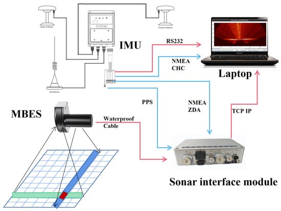
Figure 1. Data collection system. Red lines denote the types of interfaces utilized, while blue lines represent the data types and their respective directions of transmission.

The sonar device connects to the computer system via the TCP/IP protocol, transmitting the collected sonar data to the computer in real-time according to a defined data communication protocol. Simultaneously, the inertial navigation system, connected to the computer via an RS232 interface, transfers navigation data formatted according to the NMEA 0183 protocol standard. This setup ensures comprehensive and precise data acquisition, facilitating accurate underwater mapping.

In summary, the integration of PPS and ZDA data with the sonar system, along with real-time data transmission and synchronization, significantly improves the accuracy and reliability of the underwater mapping process.

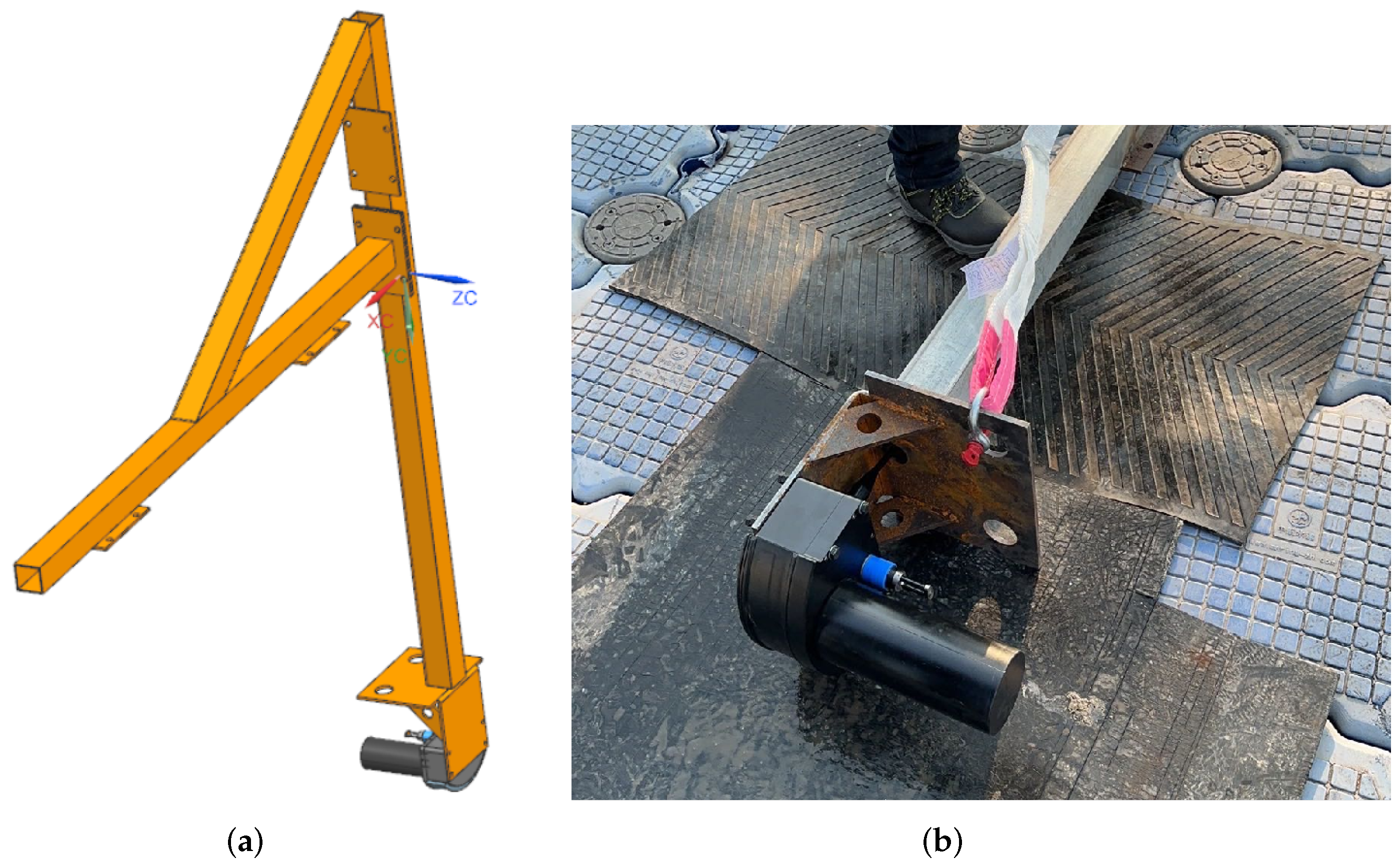
Our research is based on a sonar system designated as Model HDY-BD400D, which consists of a sonar transducer and a deck unit. As shown in Figure 2b, the sonar transducer is responsible for emitting and receiving acoustic signals and is equipped with an integrated surface sound speed probe to provide sound velocity data. Additionally, the deck unit provides power and data interfaces. The main technical parameters of this sonar system are detailed in Table 1.

Figure 2. Based on the physical model built according to the experimental vessel. (a) Mechanical structure model for the collection; (b) sonar head.

Table 1. The basic specification of the HDY-BD400D sonar.

Parameters	Value	Parameters	Value
Length	236 mm	Height	316 mm
Width	181 mm	Weight	10.9 kg
Min. frequency	400 kHz	Min.depth	1 m
Max. frequency	700 kHz	Max.depth	200 m
Pulse width	10 $\mathsf{\mu }$s–800 $\mathsf{\mu }$s	Ping rate	50 Hz
Across-track Beam width	1°	Along-track Beam width	1°
Number of Beams	256/512 (Equiangular/Equidistant)	Opening angle	10°–180°
Interface	RS232/TSS1/NMEA0183	IMU-supported	External

The INS (Table 2) is equipped with high-precision fiber optic gyroscopes, high-accuracy quartz flexural accelerometers, and an integrated mobile mapping-grade multi-mode and multi-frequency Global Navigation Satellite System (GNSS) receiver that supports the independent Beidou system. The system has been optimized for the conditions of GNSS signal obstruction and multipath interference, enabling the high-precision measurement of the moving vehicle’s heading, attitude, velocity, and position. Additionally, the system features interfaces for a variety of sensors, including GNSS, odometers, Doppler Velocity Logs (DVLs), and barometric altimeters. This versatility effectively meets the requirements for long-duration, high-precision, and high-reliability navigation in complex environments, such as urban canyons, and is suitable for the navigation and control of various unmanned systems.

Table 2. The specifications of the CHC CGI-1010 navigation sensor.

Parameters	Value
Heading accuracy (RMS)	0.05° (Dynamic alignment of a single antenna); 0.1° (Low dynamic auxiliary with dual antennas, 2 m baseline)
Pitch/Roll accuracy	0.01° (1 $\sigma$)
Velocity accuracy	0.02 m/s
Position accuracy: Single point	3 m (1 $\sigma$)
RTK	2 cm + 1 ppm (1 $\sigma$)
Gyroscope measurement range	500°/s
Gyroscope zero bias stability	0.1°/h
Accelerometer measurement range	20 g
Accelerometer zero bias stability	20 $\mathsf{\mu }$g
Maximum speed	500 m/s

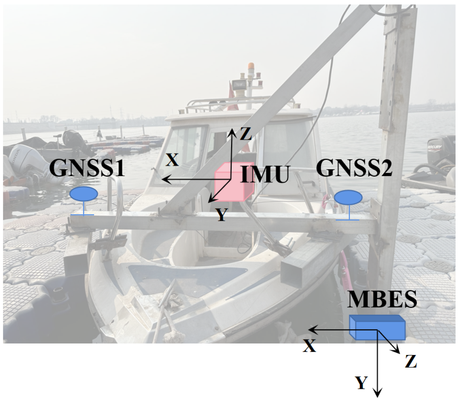
In the MBES experiment, a vessel approximately 6 m in length is used (Figure 3). The bow of the vessel is equipped with a steel railing designed for mounting stabilization brackets (Figure 2a). The sonar head is oriented at a 90-degree angle to the vessel, ensuring that acoustic signals propagate along the shortest path to the seafloor. Additionally, the sonar is positioned away from the vessel’s engine to minimize potential turbulence effects on the collected data [30].

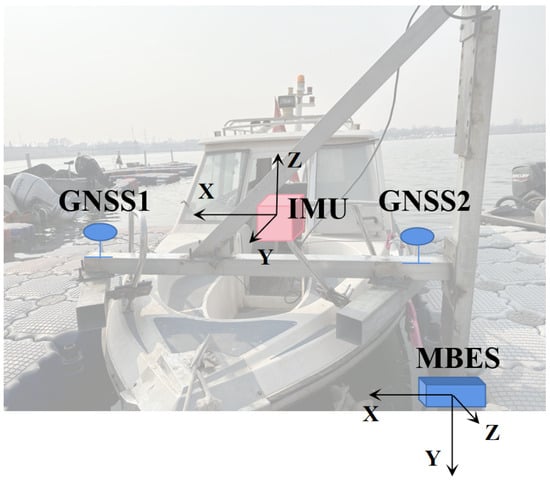
Figure 3. The relative positions of Inertial Navigation System (INS) and Multibeam echo sounder (MBES), and their respective reference coordinate systems.

2.2. Software

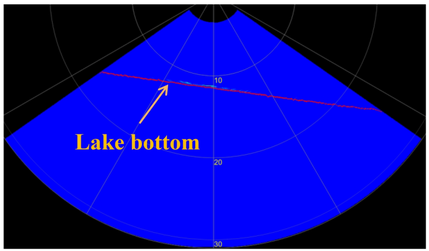
The software component primarily includes sonar parameter configuration, sonar data parsing, point cloud conversion, inertial navigation data analysis, sonar point cloud mapping, and subsequent optimization. The device drivers are independently developed under the Linux operating system. Mapping and optimization functionalities are implemented based on the ROS. The configuration of sonar parameters is crucial for acquiring high-quality sonar data. Ideal sonar data should manifest as a continuous line with clear edge beams and no significant fluctuations (Figure 4). With the other conditions held constant, different operating frequencies and pulse widths can yield significantly different sonar data. Therefore, setting appropriate sonar parameters is essential for obtaining high-quality data. Common sonar parameters are listed in Table 3. Table 4 and Figure 5 show a list of relevant topics and the tf tree used in the experiments according to our algorithm.

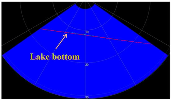
Figure 4. Appropriately selected sonar parameters yield high-quality sonar data, characterized by a stable line with minimal clutter.

Table 3. Commands that are used frequently.

Command	Range	Description
set_mode	0–2	0 = by range 1 = by depth 2 = by range and depth
set_opening_angle	10–180	Set opening angle in degrees.
set_range	0–200	Start and stop range/depth in meters
set_tx_freq	400–700	Set tx-pulse frequency in kHz
set_tx_amp	0–15	Set tx-pulse amplitude

Table 4. List of the relevant published/subscribed topics for the ROS package.

Topic	Message	Type
odom	nav_msgs/Odometry	Subscribed
nav_gpsfix	sensor_msgs/NavSatFix	Subscribed
imu_raw	sensor_msgs/Imu	Subscribed
MBES_scan	sensor_msgs/PointCloud2	Subscribed
cloud_map	sensor_msgs/PointCloud2	Published

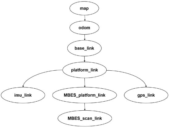
Figure 5. The ROS tf tree.

Sonar data are transmitted in the form of swath packets, with each swath containing information on the water column and bottom detection data. The $depth$ measurement from the sonar data is calculated using Formula (1).

$$depth=sample\_number\ast snd\_velocity/(2.0\ast sample\_rate)$$

(1)

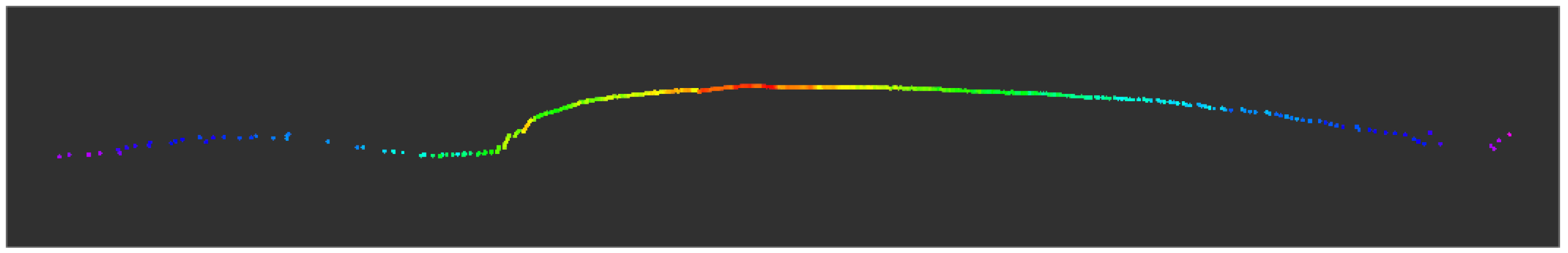
The bottom detection data within the swath packets represent the measurement results of the underwater environment by the MBES. These data can be transformed into point cloud data through the mapping of a three-dimensional matrix. The resulting point cloud data are analogous to the data from a single-line Light Detection and Ranging (LIDAR) point cloud with a fixed angle and no rotational scanning capability (Figure 6). Due to the minimal overlap between adjacent swaths and the weak association between them, frame-to-frame matching is not feasible [31]. Consequently, the direct use of the raw point cloud data from MBES for mapping does not achieve the high-precision odometry typically found in multi-line LIDAR mapping [32]. In this study, we employ the iEKF to reduce estimation errors and more accurately approach the true state of the MBES system. Furthermore, we have considered the application of the GICP algorithm for post-processing optimization to refine the point cloud data.

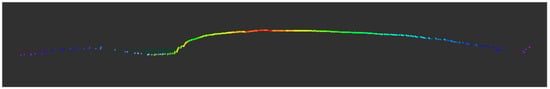
Figure 6. The single-ping point cloud recovered from sonar data, where color represents different echo intensities.

3. Methods

3.1. Mapping

MBES mapping involves integrating point cloud data with navigation information, as depicted in Figure 7. Here, the red lines represent the projection of the point cloud onto the seabed, while the black arcs depict the platform’s trajectory during motion. The resulting point cloud map consists of multiple such point clouds combined with dynamic movements. Accurate motion estimation is critical in this process.

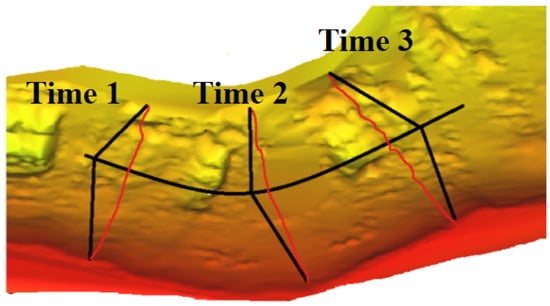
Figure 7. The process of constructing a MBES point cloud map. The red lines represent the measurements from a single ping. Time 1, Time 2, and Time 3 indicate the updates on the sonar’s position and attitude over the progression of time.

A common approach for motion estimation is based on the Kalman filter [33], where the EKF extends the standard Kalman filter through linearization [34]. However, the EKF may encounter limitations in linearizing accurately when operating far from the working point of the MBES. To address this, the iEKF assumes that both the state transition and the measurements follow nonlinear systems. It approximates the state using a linear function tangent to the nonlinear function near the mean state, aiming to iteratively refine this approximation. Additionally, the iEKF progressively reduces the correction magnitude at each iteration in the process of mapping, thereby achieving a gradual linear approximation approach toward the true state [35,36]. In summary, the iEKF offers improved performance over the EKF by better handling nonlinearities in both the state transition and the measurements, crucial for enhancing the accuracy of motion estimation in MBES mapping applications.

Assuming that the MBES data follow a Gaussian distribution, with the prior state defined as ${\tilde{x}}_k$ and the posterior state as ${\widehat{x}}_k$, we have $x\sim N(\overline{x},\sum )$, where $\overline{x}$ denotes the mean and ∑ represents the covariance matrix.

Firstly, establish a nonlinear mapping model for the MBES system’s motion, as well as a nonlinear mapping model for the measurements:

$$\begin{array}{c}{x}_k=f(x_{k-1},u_k)+w_k\\ Z_k=g\left(x_k\right)+v_k\end{array}$$

(2)

In Equation (2), $x_{k-1}$ is the state of the system at the current time step k, and $x_k$ is the predicted state at the next time step based on the current state $x_{k-1}$, as well as the control input $u_k$ and motion noise $w_k$, through the state transition function f. $v_k$ represents measurement noise.

The EKF theory mainly consists of two steps: prediction and update. During the prediction process, the previous robot state $x_{k-1}$ is recursively estimated by incorporating both the motion model and current control inputs, resulting in the prior state ${\tilde{x}}_k$ for the current time frame. In contrast, the update step focuses on computing the discrepancy between the expected measurement derived from the observation model and the actual sensor measurement. This error is utilized to adjust (correct) the prior state estimate, yielding the posterior state estimate. The prediction equation is as follows:

$$\begin{array}{c}{\tilde{x}}_k\sim N({\tilde{\mu }}_k,{{\displaystyle \tilde{\sum }}}_k),{\widehat{x}}_k\sim N({\widehat{\mu }}_k,{{\displaystyle \widehat{\sum }}}_k)\\ {{\displaystyle \tilde{\sum }}}_k=F_{k-1}{\sum }_k{F}_{k-1}^T+Q_k\\ {\tilde{\mu }}_k=f({\mu }_{k-1},u_k)\\ F_{k-1}={\displaystyle \frac{\partial {\tilde{\mu }}_k}{\partial {\mu }_{k-1}}}={\displaystyle \frac{\partial f({\mu }_{k-1},u_k)}{\partial {\mu }_{k-1}}}\end{array}$$

(3)

The update equation is as follows:

$$\begin{array}{c}{K}_k={{\displaystyle \tilde{\sum }}}_k{G}_k^T{(G_k{{\displaystyle \tilde{\sum }}}_k{G}_k^T+R_k)}^{-1}\\ {{\displaystyle \widehat{\sum }}}_k=(I-K_k{G}_k){{\displaystyle \tilde{\sum }}}_k\\ {\widehat{\mu }}_k={\tilde{\mu }}_k+K_k{E}_k={\tilde{\mu }}_k+K_k({\overline{Z}}_k-g\left({\tilde{\mu }}_k\right))\\ G_k={\displaystyle \frac{\partial g}{\partial {\tilde{\mu }}_k}}\end{array}$$

(4)

In Equation (4), $K_k$ represents the Kalman gain, which is a matrix that adjusts the covariance of the current state based on the measurement error. This helps in calibrating different sensor characteristics to determine the correction needed. ${\overline{Z}}_k,{\tilde{Z}}_k=g\left({\tilde{\mu }}_k\right)$ correspond to the actual sensor measurement and the predicted measurement based on the prior state estimate, respectively; $R_k$ denotes the covariance matrix associated with the measurement data.

Expanding upon the EKF, the iEKF enhances the update equation through an iterative process, progressively refining the posterior state estimate towards the optimal solution of the full posterior probability. The key equations are outlined as follows:

$$\begin{array}{c}{x}_{0,k}\leftarrow {\tilde{x}}_k\\ K_{op,k}={\tilde{\mu }}_k{G}_{op,k}^T{(G_{op,k}{\tilde{\mu }}_k{G}_{op,k}^T+R_k)}^{-1}\\ {{\displaystyle \widehat{\sum }}}_{op,k}=(I-K_{op,k}{G}_{op,k}){{\displaystyle \widehat{\sum }}}_{op-1,k}\\ {\widehat{\mu }}_k={\tilde{\mu }}_k+K_k({\overline{Z}}_k-g\left({\tilde{\mu }}_{op,k}\right)-G_k({\tilde{\mu }}_k-{\mu }_{op,k}))\end{array}$$

(5)

In Equation (5), the subscript “op” denotes the iteration count. At the start of each iteration, the prior state serves as the initial value for the computation. The primary distinction lies in the final line of the equation, where during each step, the correction amount corresponding to the residual after iteration is calculated, thus enhancing the optimization of the state update results.

3.1.1. IMU Recursion Step

The discrete data from an IMU can be integrated with the kinematic state equation of the vessel to estimate its state. After removing biases and compensating for gravitational acceleration from the raw IMU data, the longitudinal and lateral accelerations, along with yaw angular velocity, are represented as ${\left[\overline{a_x}\overline{a_y}w\right]}^T$. The time difference between consecutive IMU frames is denoted as $\mathsf{\Delta }{t}_k$. The vessel’s state $x_k$ is defined as follows:

$$x_k={\left[XY\phi v_x{v}_{y}w\right]}^T$$

(6)

Each component corresponds to the vessel’s horizontal position $XY$, heading $\phi$, the longitudinal velocity of the vessel’s center of mass $v_x{v}_y$, and yaw angular velocity w. The kinematic model state equation of the vessel is as follows:

$$\left[\begin{array}{c}\dot{X}\\ \dot{Y}\\ \dot{\phi }\\ \dot{v_x}\\ \dot{v_y}\end{array}\right]=\left[\begin{array}{c}{v}_{x}cos\phi -v_{y}sin\phi \\ v_{y}cos\phi +v_{x}sin\phi \\ w\\ \overline{a_x}+v_{y}w\\ \overline{a_y}-v_{x}w\end{array}\right]$$

(7)

Combining the IMU-acquired ${\left[\overline{a_x}\overline{a_y}w\right]}^T$, the nonlinear mapping equation for the prior state prediction can be obtained as follows:

$$\widetilde{{\mu }_k}={\mu }_{k-1}+\left[\begin{array}{c}(v_{x,k-1}cos{\phi }_{k-1}-v_{y,k-1}sin{\phi }_{k-1})\mathsf{\Delta }{t}_k\\ (v_{x,k-1}sin{\phi }_{k-1}-v_{y,k-1}cos{\phi }_{k-1})\mathsf{\Delta }{t}_k\\ w_{k-1}\mathsf{\Delta }{t}_k\\ (\overline{a_x}+v_{y,k-1}{W}_{k-1})\mathsf{\Delta }{t}_k\\ (\overline{a_y}-v_{x,k-1}{W}_{k-1})\mathsf{\Delta }{t}_k\\ \overline{w}-w_{k-1}\end{array}\right]$$

(8)

$${\mathit{F}}_{\mathit{k}-\mathbf{1}}=\left[\begin{array}{cccccc}1& 0& -({\widehat{v}}_{x,k-1}sin{\tilde{\phi }}_{k-1}-{\widehat{v}}_{y,k-1}cos{\widehat{\phi }}_{k-1})\mathsf{\Delta }{t}_k& \mathsf{\Delta }{t}_{k}cos{\widehat{\phi }}_{k-1}& -\mathsf{\Delta }{t}_{k}sin{\widehat{\phi }}_{k-1}& 0\\ 0& 1& ({\widehat{v}}_{x,k-1}cos{\widehat{\phi }}_{k-1}-{\widehat{v}}_{y,k-1}sin{\widehat{\phi }}_{k-1})\mathsf{\Delta }{t}_k& \mathsf{\Delta }{t}_{k}sin{\widehat{\phi }}_{k-1}& \mathsf{\Delta }{t}_{k}cos{\widehat{\phi }}_{k-1}& 0\\ 0& 0& 1& 0& 0& \mathsf{\Delta }{t}_k\\ & & & 1& 0& 0& \\ & & {\mathbf{0}}_{3\times 3}& 0& 1& 0& \\ & & & 0& 0& 0& \end{array}\right]$$

(9)

$${\mathit{V}}_k={\displaystyle \frac{\partial {\widehat{\mathit{\mu }}}_k}{\partial {\mathit{u}}_k}}=\left[\begin{array}{ccc}\hfill \hfill & \hfill {\mathbf{0}}_{3\times 3}\hfill & \\ \hfill \mathsf{\Delta }{t}_k\hfill & \hfill \hfill & \\ \hfill \hfill & \hfill \mathsf{\Delta }{t}_k\hfill & \\ \hfill \hfill & \hfill \hfill & \hfill 1\hfill \end{array}\right]$$

(10)

$${\mathit{Q}}_k={\mathit{V}}_k{\mathit{M}}_k{\mathit{V}}_k^{\mathit{T}}$$

(11)

In Equation (11), ${\mathit{M}}_k$ is the 3 × 3 covariance matrix of the IMU measurement data. Its diagonal elements correspond to the variances of longitudinal and lateral accelerations, and angular velocities, respectively. The matrix ${\mathit{F}}_{\mathit{k}}$ represents the partial derivative matrix of the state transition in the prediction equation, while ${\mathit{V}}_k$ corresponds to the partial derivative matrix of the state with respect to the incoming IMU measurements. The matrix ${\mathit{Q}}_k$ represents the covariance matrix of the state induced by the IMU measurement data in the current prediction. Once these computations are performed, the prior state prediction is completed.

3.1.2. GPS Update Step

The experiment employs a dual-antenna GPS device, hence allowing for the measurement of the heading angle between the two antennas in the W coordinate system. Therefore, the GPS-acquired data are represented as ${\overline{Z}}_G^W={\left[\begin{array}{ccc}\hfill \overline{X}\hfill & \hfill \overline{Y}\hfill & \hfill \overline{\phi }\hfill \end{array}\right]}^T$. Initialization during system startup yields the pose transformation matrix $T_M^W$ between the W and M coordinate systems. Subsequently, error calculation between the real-time measured positioning and the prior state positioning is performed, as expressed by the following formula:

$$E_G={\overline{Z}}_I^M-{\tilde{Z}}_I^M$$

(12)

$${\overline{Z}}_I^M=Log\left({\left({\overline{T}}_M^W\right)}^{-\mathbf{1}}{T}_G^W{T}_I^G\right)$$

(13)

$${\overline{T}}_G^W\leftarrow {\overline{Z}}_G^W$$

(14)

$${\tilde{Z}}_I^M=g\left({\tilde{\mu }}_k\right)=\left[\begin{array}{c}\hfill {\tilde{X}}_k\hfill \\ \hfill {\tilde{Y}}_k\hfill \\ \hfill {\tilde{\phi }}_k\hfill \end{array}\right]$$

(15)

Equation (13) converts the coordinate and directional vectors into a pose transformation matrix. This matrix is used to project the coordinates obtained from the GPS into the W coordinate system onto the map. Subsequently, the residual is calculated by comparing these projected coordinates with the prior positioning of the current vessel on the map. This residual is then incorporated into the update formula to adjust the prior state. This step aims to refine the vessel’s positioning within the W system, thereby enhancing the absolute positioning accuracy of the system.

3.2. Point Cloud Registration

For feature matching, loop closure detection, and the integration of data collected at different times, we performed point cloud registration operations, which are essential for ensuring data consistency and enhancing the accuracy of map construction. In this section, we focus on registering local point cloud maps using the GICP [28,37]. The GICP algorithm facilitates point-to-point, point-to-plane, or plane-to-plane matching by reformulating the error function as a probability distribution model, where sampled points are represented as Gaussian distributions. Assuming point clouds P and Q follow Gaussian distributions:

$$\begin{array}{cc}\hfill & \hfill p_i\sim N\left(p_i,C_i^P\right)\hfill \\ \hfill & \hfill q_i\sim N\left(q_i,C_i^Q\right)\hfill \end{array}$$

(16)

where $C_i^P$ and $C_i^Q$ represent the covariance matrices of P and Q, respectively, and let $q_i=T*p_i$, where $T*$ represents the transformation matrix. Therefore, the error function can be rewritten as:

$$E=q_i-T*p_i=f\left(T*\right)$$

(17)

From the properties of Gaussian distribution, the probability distribution of E is given by:

$$E\sim N\left(q_i-T*p_i,C_i^Q+T^{\ast }{C}_i^P{\left(T^{\ast }\right)}^T\right)=N\left(0,C_i^Q+T^{\ast }{C}_i^P{\left(T^{\ast }\right)}^T\right)$$

(18)

Find the maximum likelihood transformation $T*$ that maximizes the logarithm of the above expression, resulting in the following objective function:

$$\begin{array}{cc}\hfill T^{\ast }& \hfill =\underset{T^{\ast }}{argmax}\mathsf{\Pi }p\left({\left(E\right)}^T\right)=\underset{T^{\ast }}{argmax}\sum _{i}ln\left[p\left({\left(E\right)}^T\right)\right]\hfill \\ \hfill & \hfill =\underset{T^{\ast }}{argmin}\sum _i{\left(E\right)}^T·{\left(C_i^Q+T^{\ast }{C}_i^P{\left(T^{\ast }\right)}^T\right)}^{-1}·E\hfill \end{array}$$

(19)

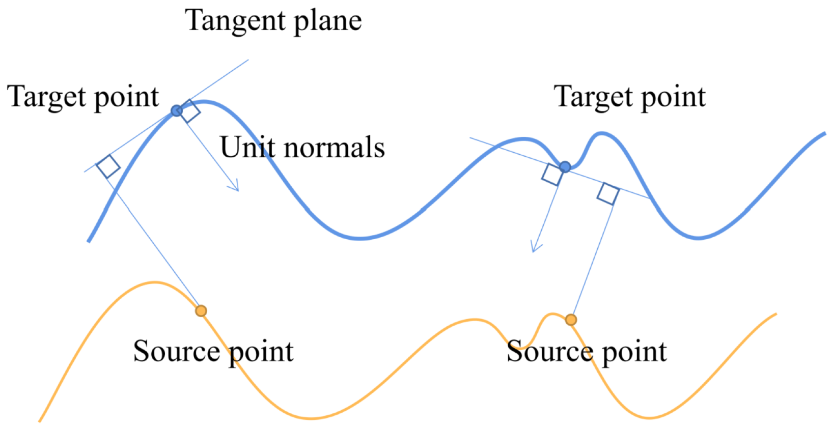
The objective function is solved using an unconstrained non-optimization method from the Point Cloud Library (PCL) to determine the optimal values for the transformation matrix $T*$. GICP analyzes the local properties of each pair of original points and target points to adjust the weights of the generated distance residuals. This weight is represented by the coefficient $P_i=C_i^{\varrho }+T^{\ast }{C}_i^p{\left(T^{\ast }\right)}^T$ in the quadratic form concerning distance. When $P_i$ is an identity matrix, GICP degenerates to the most common point-to-point registration. In the case where all points in $T^{\ast }{P}_i$ are closest to the corresponding tangent plane of the target point $q_i$, GICP performs point-to-plane matching (Figure 8).

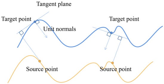
Figure 8. Generalized Iterative Closest Point (GICP) algorithm for point-to-plane registration. Blue represents the target surface, and yellow represents the source point cloud.

4. Experiments and Results

4.1. Experimental Description

To validate the practicality and reliability of our approach, we conducted field experiments at Li Quan Lake (Xi’an, Shaanxi Province, China). The experimental environment is geographically located at 34°31′29″ N, 108°25′31″ E, with the test area measuring approximately 350 × 200 m. The vessel moved along a serpentine route, with an overlap rate between adjacent survey lines ranging from 30% to 50%, as shown in Figure 9. The water depth near the shore averages approximately 8 m, while the depth at the lake’s center reaches about 12 m. The experimental vessel maintained an average speed of 2 knots throughout the survey.

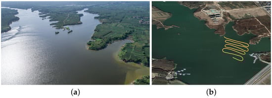
Figure 9. Environment and satellite map of experiments performed. (a) Aerial view; (b) satellite map.

To verify the accuracy of the map construction and to prepare datasets for future underwater target detection tasks, we have fabricated cylindrical, cubic, and human-shaped models as bottom targets. Examples of these models are illustrated in Figure 10. During target deployment, utilize the mobile phone’s built-in GPS to record the latitude and longitude coordinates of the deployment site. This will ensure accurate matching and comparison of the collected target point cloud data with the actual geographical location.

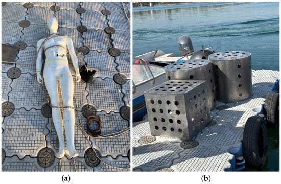
Figure 10. Underwater target objects. (a) Human-shaped model; (b) cube and cylinder.

The sonar parameters used during the experimental process are outlined in Table 5. Particularly, the near-field threshold parameter is set to efficiently filter out noise that may occur in close proximity to the sonar head.

Table 5. The sonar parameters used in the experiments.

Parameters	Value	Parameters	Value
Frequency	400 khz	Range	20 m
Pulse width	240 $\mathsf{\mu }$s	Transmission amplitude	7
Sound velocity	1486 m/s	Bandwidth	80 kHz
Near-field Threshold	1	Beamwidth	150

4.2. Mapping Results

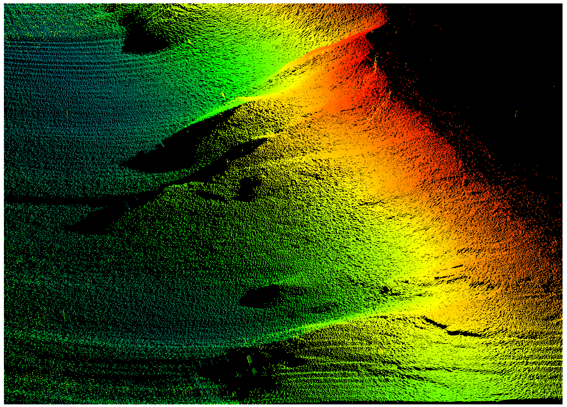
Figure 11 presents the point cloud results visualized using RVIZ [38], the Robot Visualization tool widely utilized for 3D visualization in robotics and autonomous systems. Specifically, the left image depicts the scan conducted near the center of the lake, where the lakebed is relatively flat, devoid of significant targets, and the vessel’s movement is slow. In contrast, the right image is scanned near a cliff wall, where the lakebed exhibits a natural gradient. The distribution of the point cloud is asymmetric, revealing an accumulation of debris near the wall. Additionally, the protrusion on the right side of the point cloud image corresponds to the recessed shape of the cliff wall. Figure 12 presents the scan results of a nearshore lakebed terrain, where loess deposits from the shore have settled onto the lakebed, creating undulating slopes.

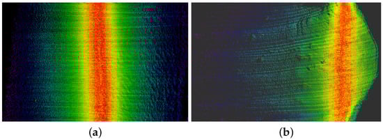
Figure 11. The scanning results displayed within the RVIZ interface. The left image presents the scan outcomes of a flat terrain, whereas the right image depicts a sloping terrain with obstructions caused by mountainous features. (a) Flat terrain; (b) sloping terrain.

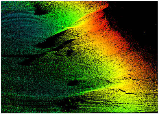
Figure 12. The scanning results of the lakebed terrain.

4.3. Target Scanning Results

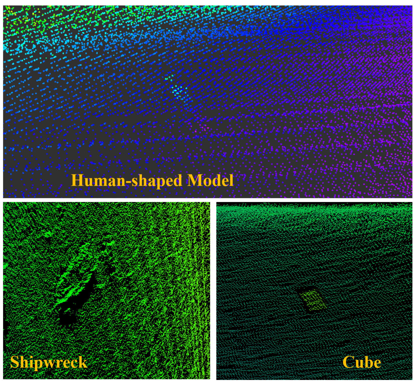
Figure 13 displays the scanning results of underwater targets and a shipwreck on the lakebed obtained in this experiment. The positions of the targets were precisely recorded with latitude and longitude coordinates (Table 6). Subsequently, the experimental vessel passed through the target deployment area to facilitate locating and identifying these targets. It is noteworthy that due to the limited number of experimental samples, we have not observed significant differences in detection performance among different shapes of objects. Factors such as object depth and sediment burial appear to have a more pronounced impact on detection results.

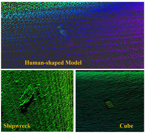
Figure 13. The scanning results of underwater targets and shipwreck.

Table 6. The target location of the deployment and its distinguishability in MBES point cloud.

Target	Placement Longitude	Placement Latitude	Depth	Is Discernible in This Experiment
Human-shaped model	108.42743301	34.52545100	8.17 m	YES
Cylinder	108.42626401	34.52634600	10.12 m	NO
Cube	108.42716101	34.52620700	8.90 m	YES

4.4. Registration Results

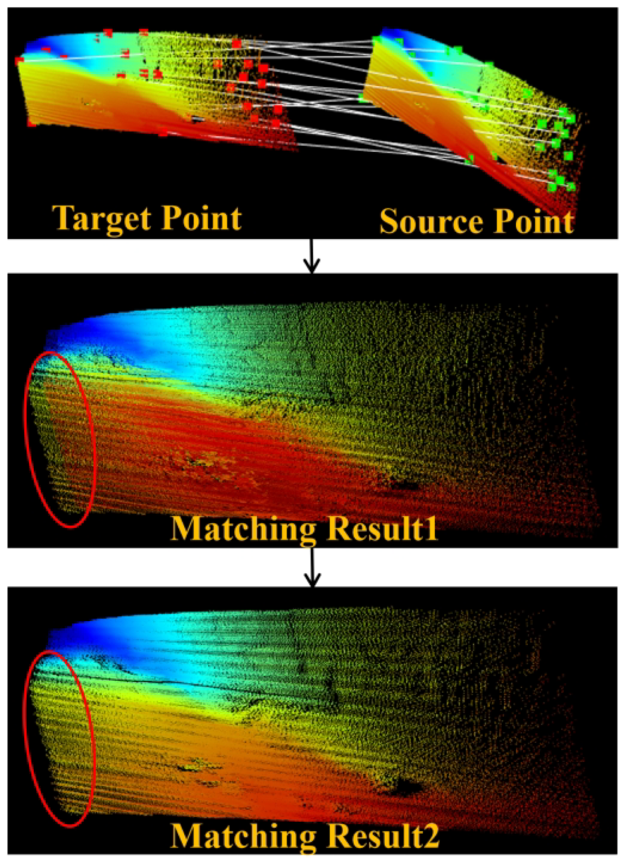
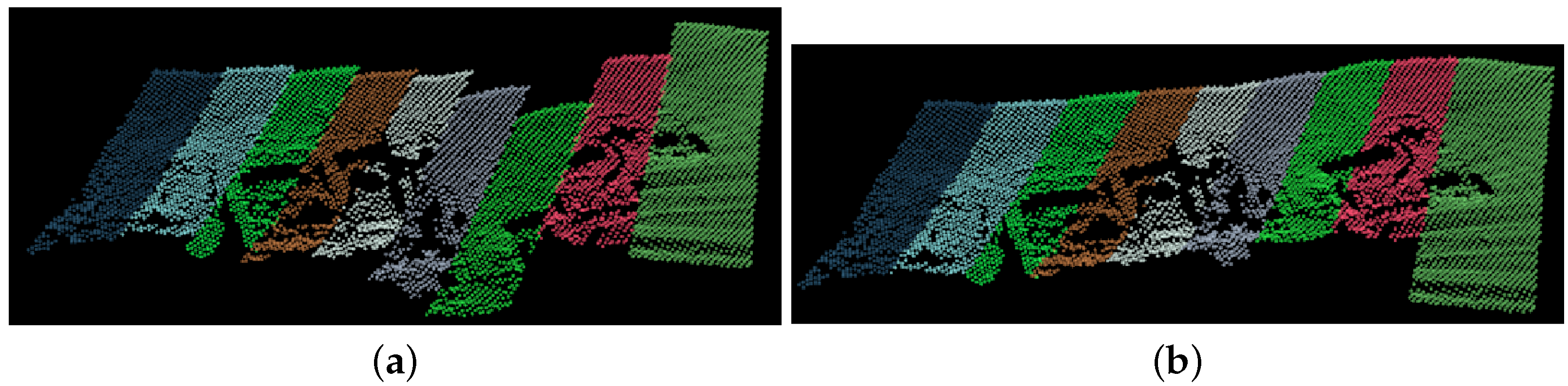
Figure 14 illustrates the detailed process of registering a subset of point cloud data, which includes feature extraction, the computation of feature correspondences, coarse matching, and subsequent refinement using the GICP algorithm. Initially, random transformations and Gaussian noise are applied to the loaded point cloud map to simulate real-world scenarios. Key features are then identified within the input point cloud using the Harris Corner Detector, and correspondences between these key points are computed. A coarse matching of the point clouds is performed using the estimated rigid transformation. To enhance registration accuracy, the GICP algorithm is employed for a refined matching phase, effectively managing nonlinear transformations and achieving the precise alignment of the point cloud data despite significant noise interference. The experiment indicates that the average registration error of the algorithm is 0.97 m. Furthermore, Figure 15 depicts a scenario with more distinct features, where the average registration error is further reduced.

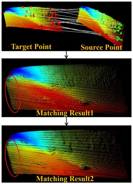
Figure 14. The result of registering two MBES point clouds. The first registration aligns the noisy and randomly transformed point cloud with the original point cloud using an estimated rigid transformation, aiming to eliminate noise and align the two point clouds. The second registration further improves the registration accuracy using the GICP algorithm, which is performed after the first registration. The arrow represents the continuous registration process, and the effect contrast of registration can be clearly seen at the red circle.

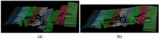
Figure 15. The result of the registration of a clearly defined underwater target with regular lines and edges. (a) Before registration; (b) after registration.

5. Discussion

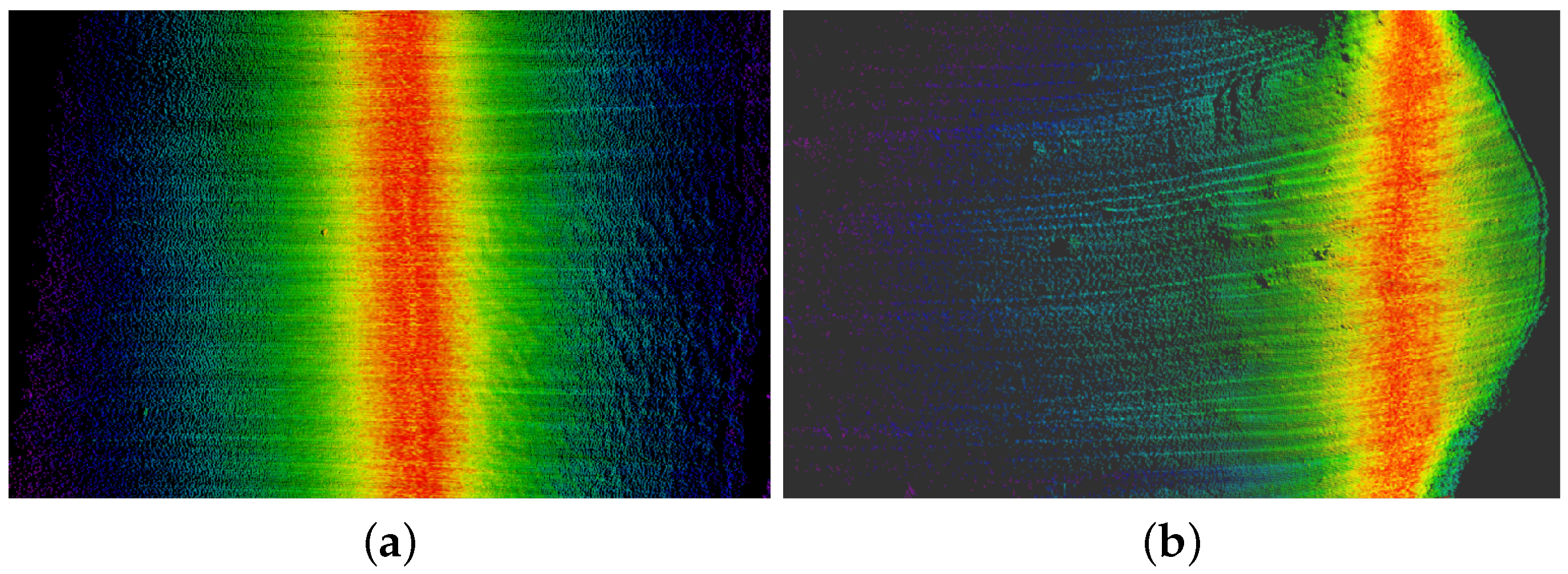
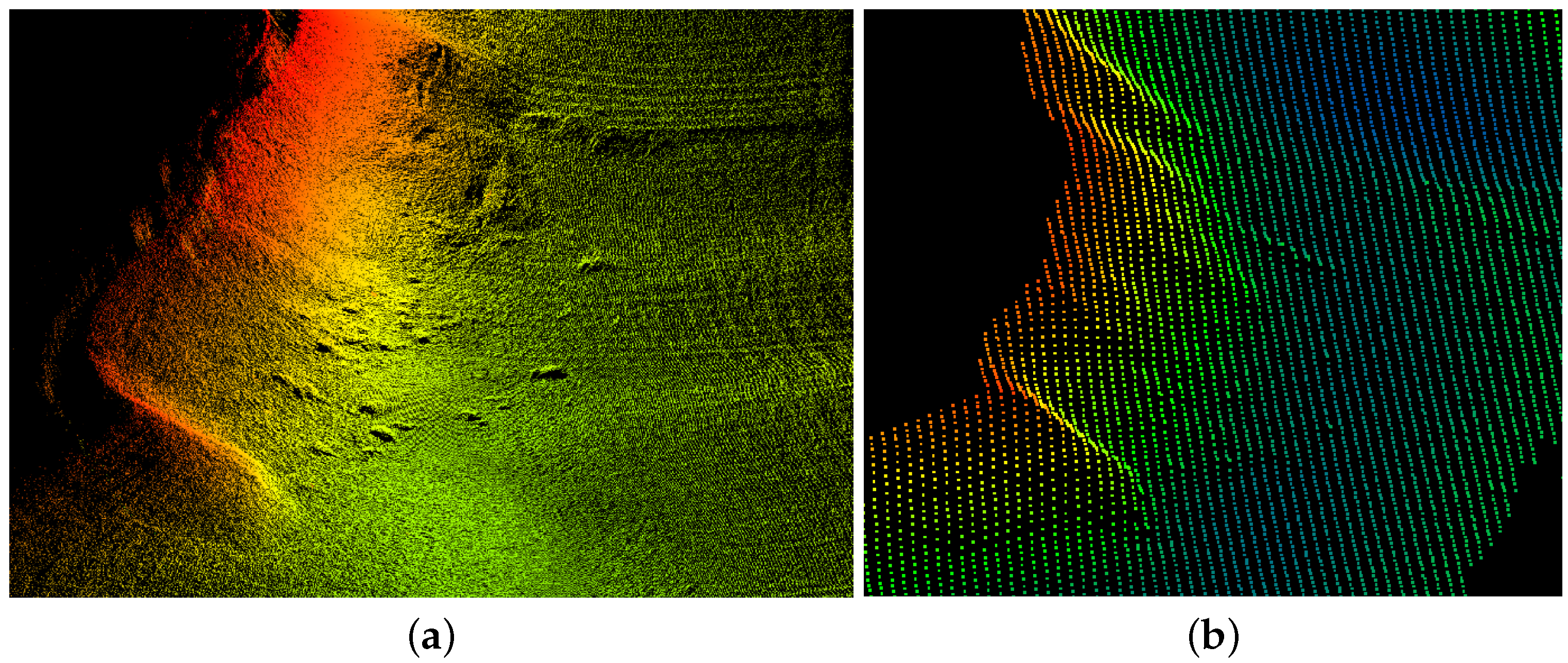
The real-time scanned data are exported as point cloud files with the .pcd suffix, which facilitates efficient viewing and analysis in the CloudCompare software [39]. Figure 16 shows an example of the point cloud data as viewed in CloudCompare. The point cloud files exported using the HydroMaster have been processed to remove noise, but this processing has also resulted in the loss of a significant amount of original information. In contrast, our mapping algorithm retains the original data, allowing for more precise analysis. Specifically, our algorithm increases the scan width by one-third at the same scanning distance, and the number of point clouds is 1000 times greater than that processed with the HydroMaster.

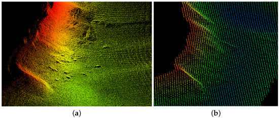
Figure 16. The algorithm proposed in this study (left), and the other produced by the HydroMaster (right). Both images are the result of scanning the same terrain at different times. The advantage of our method lies in its ability to export point cloud files with greater information content, preserving more detailed features. In contrast, the point cloud data exported by the HydroMaster software may lose some details due to the sampling process. The data can be accessed at http://www.hydroshare.org/resource/3592c1d35fdb4f29a1416e2c6099e13b (accessed on 6 July 2024). (a) Our method; (b) HydroMaster.

Figure 17 illustrates the analysis of the trajectory estimation error. During the experiment, the vessel traveled approximately 1700 m in total, with the GPS-provided values serving as the ground truth. Absolute Trajectory Error (ATE) is commonly used as a metric to evaluate mapping quality in SLAM applications. This metric was first proposed by [40], and in [9,41] it has been utilized to assess MBES mapping performance. The authors of [9] compare ATE values for MBES mapping using three different algorithms, showing a maximum ATE of up to 90 m. Our results indicate that the iEKF method achieved an ATE of 15.10 m, whereas the EKF method resulted in an ATE of 16.91 m, which demonstrates the effectiveness of our approach. Throughout the experiment, errors were notably larger during turns and relatively smaller during straight-line travel. The experimental results are shown in Table 7, where “Location error of human-shaped model” and “Location error of cube” are derived from the difference between the scanned locations and the actual locations of the targets. A comparative analysis indicates that our approach has significantly enhanced the reliability and accuracy of map construction. Furthermore, the application of the GICP algorithm for point cloud registration has resulted in a reduction of the ATE by 9.0%.

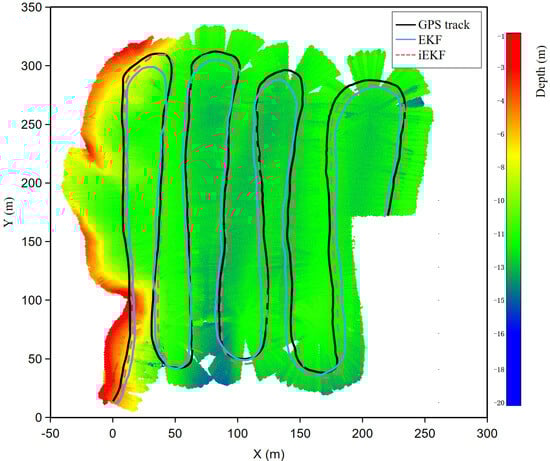
Figure 17. Estimated trajectory of the vessel.

Table 7. The experimental results.

Method	ATE (m)	Trajectory Error at Turns (m)	Trajectory Error of Straight-Line Driving (m)	Average Registration Error (m)	Location Error of Human-Shaped Model (m)	Location Error of Cube (m)
HydroMaster	14.65	15.17	14.57	× 1	3.89	5.50
EKF	16.91	17.75	16.67	×	4.35	6.31
iEKF	15.10	16.81	14.93	×	3.96	5.63
EKF + GICP	15.38	15.71	15.25	1.34	4.23	6.17
iEKF + GICP(ours)	13.74	14.03	13.57	0.97	3.77	5.46

¹ This symbol indicates that the verification of the corresponding metric cannot be carried out.

6. Conclusions

This study presents a method for underwater mapping and optimization based on MBES. Initially, an MBES data acquisition system is established, achieving stable data collection and playback functions. Subsequently, a preliminary mapping method based on iEKF is developed, followed by point cloud registration using GICP. The results from the lake experiments indicate that our method exhibits satisfactory performance in underwater mapping and point registration, with a 6.2% reduction in the ATE and a 9.0% reduction in average error after point cloud registration optimization. Additionally, our method also achieved the best performance in terms of resolving errors at the deployed prefabricated target positions. Looking forward, our future plans include manufacturing a series of prototype target objects to deploy in the experimental area for detection. This initiative aims to collect and analyze more real-world data. All relevant detection data and results will be publicly shared to facilitate further research and discussion within the scientific community. Moreover, we intend to integrate the MBES system with Unmanned Underwater Vehicles (UUVs), which will significantly enhance the intelligence and operational efficiency of detection missions.

References

- Mao, Z.; Zhang, Z. Taking the “UN Decade of Ocean Science for Sustainable Development” as an opportunity to help build a “Community with a Shared Future between China and Pacific Island Countries”. Mar. Policy 2024, 159, 105943. [Google Scholar] [CrossRef]
- Huy, D.Q.; Sadjoli, N.; Azam, A.B.; Elhadidi, B.; Cai, Y.; Seet, G. Object perception in underwater environments: A survey on sensors and sensing methodologies. Ocean Eng. 2023, 267, 113202. [Google Scholar] [CrossRef]
- Yan, Z.; Min, X.; Xu, D.; Geng, D. A novel method for underactuated UUV tracking unknown contour based on forward-looking sonar. Ocean Eng. 2024, 301, 117545. [Google Scholar] [CrossRef]
- Zhang, J.; Xie, Y.; Ling, L.; Folkesson, J. A fully-automatic side-scan sonar simultaneous localization and mapping framework. IET Radar Sonar Navig. 2024, 18, 674–683. [Google Scholar] [CrossRef]
- Bore, N.; Folkesson, J. Neural shape-from-shading for survey-scale self-consistent bathymetry from sidescan. IEEE J. Ocean. Eng. 2022, 48, 416–430. [Google Scholar] [CrossRef]
- Rizzo, A.; De Giosa, F.; Donadio, C.; Scardino, G.; Scicchitano, G.; Terracciano, S.; Mastronuzzi, G. Morpho-bathymetric acoustic surveys as a tool for mapping traces of anthropogenic activities on the seafloor: The case study of the Taranto area, southern Italy. Mar. Pollut. Bull. 2022, 185, 114314. [Google Scholar] [CrossRef] [PubMed]
- Scardino, G.; De Giosa, F.; D’Onghia, M.; Demonte, P.; Fago, P.; Saccotelli, G.; Valenzano, E.; Moretti, M.; Velardo, R.; Capasso, G.; et al. The footprints of the wreckage of the Italian royal navy battleship leonardo da vinci on the mar piccolo sea-bottom (Taranto, Southern Italy). Oceans 2020, 1, 77–93. [Google Scholar] [CrossRef]
- Instruments, L.C.S. Multibeam Sonar Theory of Operation, 1st ed.; L-3 Communications SeaBeam Instruments: Boston, MA, USA, 2000. [Google Scholar]
- Teng, M.; Ye, L.; Yuxin, Z.; Zhang, Q.; Jiang, Y.; Zheng, C.; Zhang, T. Robust bathymetric SLAM algorithm considering invalid loop closures. Appl. Ocean Res. 2020, 102, 102298. [Google Scholar]
- Ji, X.; Yang, B.; Tang, Q. Acoustic seabed classification based on multibeam echosounder backscatter data using the PSO-BP-AdaBoost algorithm: A case study from Jiaozhou Bay, China. IEEE J. Ocean. Eng. 2020, 46, 509–519. [Google Scholar] [CrossRef]
- Trzcinska, K.; Janowski, L.; Nowak, J.; Rucinska-Zjadacz, M.; Kruss, A.; von Deimling, J.S.; Pocwiardowski, P.; Tegowski, J. Spectral features of dual-frequency multibeam echosounder data for benthic habitat mapping. Mar. Geol. 2020, 427, 106239. [Google Scholar] [CrossRef]
- Maleika, W.; Forczmański, P. Adaptive modeling and compression of bathymetric data with variable density. IEEE J. Ocean. Eng. 2019, 45, 1353–1369. [Google Scholar] [CrossRef]
- Seaman, P.; Sturkell, E.; Gyllencreutz, R.; Stockmann, G.J.; Geirsson, H. New multibeam mapping of the unique Ikaite columns in Ikka Fjord, SW Greenland. Mar. Geol. 2022, 444, 106710. [Google Scholar] [CrossRef]
- Wang, J.; Tang, Y.; Jin, S.; Bian, G.; Zhao, X.; Peng, C. A Method for Multi-Beam Bathymetric Surveys in Unfamiliar Waters Based on the AUV Constant-Depth Mode. J. Mar. Sci. Eng. 2023, 11, 1466. [Google Scholar] [CrossRef]
- Yan, Z.; Zhou, T.; Guo, Q.; Xu, C.; Wang, T.; Peng, D.; Yu, X. Terrain matching positioning method for underwater vehicles based on curvature discrimination. Ocean Eng. 2022, 260, 111965. [Google Scholar] [CrossRef]
- Melo, J.; Matos, A. Survey on advances on terrain based navigation for autonomous underwater vehicles. Ocean Eng. 2017, 139, 250–264. [Google Scholar] [CrossRef]
- Zhang, H.; Zhang, S.; Wang, Y.; Liu, Y.; Yang, Y.; Zhou, T.; Bian, H. Subsea pipeline leak inspection by autonomous underwater vehicle. Appl. Ocean Res. 2021, 107, 102321. [Google Scholar] [CrossRef]
- Weber, T.C. A CFAR detection approach for identifying gas bubble seeps with multibeam echo sounders. IEEE J. Ocean. Eng. 2021, 46, 1346–1355. [Google Scholar] [CrossRef]
- Bello, J.; Eriksen, P.; Pocwiardowski, P. Oil leak detections with a combined telescopic fluorescence sensor and a wide band multibeam sonar. In Proceedings of the International Oil Spill Conference Proceedings. International Oil Spill Conference, Long Beach, CA, USA, 15–18 May 2017; pp. 1559–1573. [Google Scholar]
- Ghobrial, M. Fish Detection Automation from ARIS and DIDSON SONAR Data. Master’s Thesis, University of Oulu, Degree Programme in Computer Science and Engineering, Oulu, Finland, 2019. [Google Scholar]
- Solana Rubio, S.; Salas Romero, A.; Cerezo Andreo, F.; González Gallero, R.; Rengel, J.; Rioja, L.; Callejo, J.; Bethencourt, M. Comparison between the employment of a multibeam echosounder on an unmanned surface vehicle and traditional photogrammetry as techniques for documentation and monitoring of shallow-water cultural heritage sites: A case study in the bay of Algeciras. J. Mar. Sci. Eng. 2023, 11, 1339. [Google Scholar] [CrossRef]
- Jung, J.; Lee, Y.; Park, J.; Yeu, T.K. Multi-modal sonar mapping of offshore cable lines with an autonomous surface vehicle. J. Mar. Sci. Eng. 2022, 10, 361. [Google Scholar] [CrossRef]
- Thoms, A.; Earle, G.; Charron, N.; Narasimhan, S. Tightly Coupled, Graph-Based DVL/IMU Fusion and Decoupled Mapping for SLAM-Centric Maritime Infrastructure Inspection. IEEE J. Ocean. Eng. 2023, 48, 663–676. [Google Scholar] [CrossRef]
- Li, S.; Su, D.; Yang, F.; Zhang, H.; Wang, X.; Guo, Y. Bathymetric LiDAR and multibeam echo-sounding data registration methodology employing a point cloud model. Appl. Ocean Res. 2022, 123, 103147. [Google Scholar] [CrossRef]
- Stateczny, A.; Gronska, D.; Wlodarczyk-Sielicka, M.; Motyl, W. Multibeam echosounder and LiDAR in process of 360O numerical map production for restricted waters with HydroDron. In Proceedings of the 2018 Baltic Geodetic Congress (BGC Geomatics), Olsztyn, Poland, 21–23 June 2018; pp. 288–292. [Google Scholar]
- Han, J.; Kim, J. Three-dimensional reconstruction of a marine floating structure with an unmanned surface vessel. IEEE J. Ocean. Eng. 2018, 44, 984–996. [Google Scholar] [CrossRef]
- Krasnosky, K.; Roman, C. A massively parallel implementation of Gaussian process regression for real time bathymetric modeling and simultaneous localization and mapping. Field Robot. 2022, 2, 940–970. [Google Scholar] [CrossRef]
- Torroba, I.; Sprague, C.I.; Bore, N.; Folkesson, J. PointNetKL: Deep inference for GICP covariance estimation in bathymetric SLAM. IEEE Robot. Autom. Lett. 2020, 5, 4078–4085. [Google Scholar] [CrossRef]
- Tan, J.; Torroba, I.; Xie, Y.; Folkesson, J. Data-driven loop closure detection in bathymetric point clouds for underwater slam. In Proceedings of the 2023 IEEE International Conference on Robotics and Automation (ICRA), London, UK, 29 May–2 June 2023; IEEE: Piscataway, NJ, USA, 2023; pp. 3131–3137. [Google Scholar]
- Constantinoiu, L.F.; Bernardino, M.; Rusu, E. Autonomous Shallow Water Hydrographic Survey Using a Proto-Type USV. J. Mar. Sci. Eng. 2023, 11, 799. [Google Scholar] [CrossRef]
- Ling, Y.; Li, Y.; Ma, T.; Cong, Z.; Xu, S.; Li, Z. Active Bathymetric SLAM for autonomous underwater exploration. Appl. Ocean Res. 2023, 130, 103439. [Google Scholar] [CrossRef]
- Khan, M.U.; Zaidi, S.A.A.; Ishtiaq, A.; Bukhari, S.U.R.; Samer, S.; Farman, A. A comparative survey of lidar-slam and lidar based sensor technologies. In Proceedings of the 2021 Mohammad Ali Jinnah University International Conference on Computing (MAJICC), Karachi, Pakistan, 15–17 July 2021; IEEE: Piscataway, NJ, USA, 2021; pp. 1–8. [Google Scholar]
- Ribeiro, M.I. Kalman and extended kalman filters: Concept, derivation and properties. Inst. Syst. Robot. 2004, 43, 3736–3741. [Google Scholar]
- Krasnosky, K.; Roman, C.; Casagrande, D. A bathymetric mapping and SLAM dataset with high-precision ground truth for marine robotics. Int. J. Robot. Res. 2022, 41, 12–19. [Google Scholar] [CrossRef]
- Bi, S.; Zhang, B.; Li, J.; Xu, Y. Map Boundary Optimization Based on Adaptive Iterative Extended Kalman Filter. In Proceedings of the 2022 41st Chinese Control Conference (CCC), Hefei, China, 25–27 July 2022; IEEE: Piscataway, NJ, USA, 2022; pp. 2979–2983. [Google Scholar]
- Xu, W.; Zhang, F. Fast-lio: A fast, robust lidar-inertial odometry package by tightly-coupled iterated kalman filter. IEEE Robot. Autom. Lett. 2021, 6, 3317–3324. [Google Scholar] [CrossRef]
- Koide, K.; Yokozuka, M.; Oishi, S.; Banno, A. Voxelized gicp for fast and accurate 3d point cloud registration. In Proceedings of the 2021 IEEE International Conference on Robotics and Automation (ICRA), Xi’an, China, 30 May–5 June 2021; IEEE: Piscataway, NJ, USA, 2021; pp. 11054–11059. [Google Scholar]
- Kam, H.R.; Lee, S.H.; Park, T.; Kim, C.H. Rviz: A toolkit for real domain data visualization. Telecommun. Syst. 2015, 60, 337–345. [Google Scholar] [CrossRef]
- Girardeau-Montaut, D. CloudCompare. In Proceedings of the 2nd International Workshop on Point Cloud Processing, Stuttgart, Germany, 4–5 December 2019; Available online: https://www.eurosdr.net/sites/default/files/images/inline/04-cloudcompare_pcp_2019_public.pdf (accessed on 9 July 2024).
- Schubert, D.; Goll, T.; Demmel, N.; Usenko, V.; Stückler, J.; Cremers, D. The TUM VI benchmark for evaluating visual-inertial odometry. In Proceedings of the 2018 IEEE/RSJ International Conference on Intelligent Robots and Systems (IROS), Madrid, Spain, 1–5 October 2018; IEEE: Piscataway, NJ, USA, 2018; pp. 1680–1687. [Google Scholar]
- Teng, M.; Ye, L.; Yuxin, Z.; Yanqing, J.; Qianyi, Z.; Pascoal, A.M. Efficient bathymetric SLAM with invalid loop closure identification. IEEE/ASME Trans. Mechatron. 2020, 26, 2570–2580. [Google Scholar] [CrossRef]
Disclaimer/Publisher’s Note: The statements, opinions and data contained in all publications are solely those of the individual author(s) and contributor(s) and not of MDPI and/or the editor(s). MDPI and/or the editor(s) disclaim responsibility for any injury to people or property resulting from any ideas, methods, instructions or products referred to in the content. |
© 2024 by the authors. Licensee MDPI, Basel, Switzerland. This article is an open access article distributed under the terms and conditions of the Creative Commons Attribution (CC BY) license (https://creativecommons.org/licenses/by/4.0/).