The Role of Tide and Wind in Modulating Density Stratification in the Pearl River Estuary during the Dry Season

Abstract

Density stratification plays a crucial role in estuarine hydrodynamics and material transport. In this study, we utilized a well-calibrated numerical model to investigate the stratification processes and underlying mechanisms in the dynamically wide Pearl River Estuary (PRE). In the upper estuary, longitudinal straining governs stratification, enhancing it during ebb tide and reducing it during flood tide. The Coriolis force becomes significant in the lower estuary due to the increased basin width, causing seaward freshwater to be confined to the West Shoal, where a pronounced transverse salinity gradient forms. Interacting with lateral current shear, density stratification is most pronounced in this region. The prevailing northeasterly wind creates a mixed layer near the surface, shifting stratification to the middle layer of the water column in the upper estuary. Wind stirring reduces stratification throughout the estuary. Under the wind’s influence, the seaward outflow is confined to a narrower region and shifts westward, resulting in the most apparent stratification occurring on the West Shoal of the PRE due to lateral straining. These findings on the evolution of freshwater pathways and their role in modulating density stratification have significant implications for other wide estuaries, such as Delaware Bay and the La Plata-Parana estuary.

1. Introduction

Density stratification significantly influences the hydrodynamics, material transport, and ecosystem health of estuaries. It is a critical factor affecting the strength of estuarine circulation [1], suppressing sediment suspension height [2], and influencing primary production and hypoxia levels [3]. Thus, a thorough examination of stratification and its controlling mechanisms is essential for comprehending the hydrodynamic and biochemical processes within estuarine systems.

The stratification processes in estuaries have been extensively investigated through both in-situ measurements and numerical modeling. Simpson et al. [4] elucidated that tidal straining, arising from the interaction between vertical shear and longitudinal salinity gradients, induces periodic stratification during the flood-ebb cycle. Burchard and Hofmeister [5], through their examination of the time-dependent equation of potential energy anomalies, determined that variations in stratification stem from the interplay between tidal straining and vertical mixing. This theory has been corroborated by numerous observational studies in estuaries such as the Changjiang Estuary [6], the York River Estuary [7], and the Guadiana Estuary [8]. Transversely, the interaction between vertical shear in lateral flows and transverse salinity gradients can generate lateral straining, which predominantly governs stratification during the latter part of the flood tide [9,10]. Hence, it is imperative to consider three-dimensional hydrodynamics when investigating the stratification and destratification processes in an estuary.

In addition to tides, winds significantly influence estuarine hydrodynamics and density stratification. In shallow coastal areas, strong winds can thoroughly mix the water column, redistributing dissolved oxygen. Wind forcing also alters vertical shear and salinity transport, thereby modulating stratification. Scully et al. [11] demonstrated that down-estuary winds enhance vertical shear, which interacts with longitudinal salinity gradients to increase stratification, while up-estuary winds reduce vertical shear, leading to decreased stratification. Chen and Sanford [12] observed that density stratification initially increases and then decreases with increasing down-estuary wind, revealing that the impact of wind on stratification is determined by the competition between wind straining and direct wind mixing. Li and Li [13] suggested that wind-driven lateral straining is not in phase with longitudinal straining, causing asymmetry in the modulation of stratification between down-estuary and up-estuary winds. Moderate down-estuary winds also reinforce the two-layer estuarine circulation, enhancing seaward freshwater transport at the surface and landward saline water near the bottom, resulting in a strong vertical salinity gradient [14]. However, the structure of estuarine circulation can vary significantly depending on estuary width and friction [15]. In wide estuaries (where the Kevin number > 1, $K_e=Bf/\sqrt{g^{\prime }{h}_s}$, where B represents the estuary width, $g^{\prime }$ is the reduced gravity, $h_s$ is the mean depth of the buoyant layer, and f is the Coriolis parameter), freshwater is transported seaward along the right side (looking downstream) of the estuary, while high-salinity water is transported landward on the opposite side [16]. Wind can alter this circulation structure, leading to a redistribution of salinity [17,18]. To the best of our knowledge, the response of stratification to the combined influence of wind and tide in wide estuaries (Kelvin number > 1) has seldom been investigated. The stratification processes and underlying mechanisms, influenced by the combined effects of tides and winds in wide estuaries, remain poorly understood.

The Pearl River Estuary (PRE) exemplifies a dynamically wide estuary, with the Kelvin number ranging from less than 1 near the Humen Outlet to approximately 8 near the estuary mouth. This variation signifies the increasing influence of the Coriolis effect on estuarine hydrodynamics as the estuary broadens [19]. As the width of the estuary expands, the estuarine circulation adopts a laterally sheared structure, characterized by seaward outflow on the western side and landward inflow constrained to the eastern side [20]. Consequently, a substantial portion of river-borne sediment is transported to the western part of the estuary [21]. Additionally, the hydrodynamics of the PRE are significantly influenced by the seasonal monsoon climate, with the prevailing northeasterly wind during the dry season enhancing estuarine circulation [22]. While the estuarine circulation in both longitudinal and transverse directions has been extensively studied, the effects of these changes on stratification remain poorly understood. In this study, we first elucidate how estuarine hydrodynamics are modulated by winds. Subsequently, we examine the stratification processes and their underlying mechanisms. This study aims to enhance our understanding of hydrodynamics in the PRE and other wide estuaries worldwide.

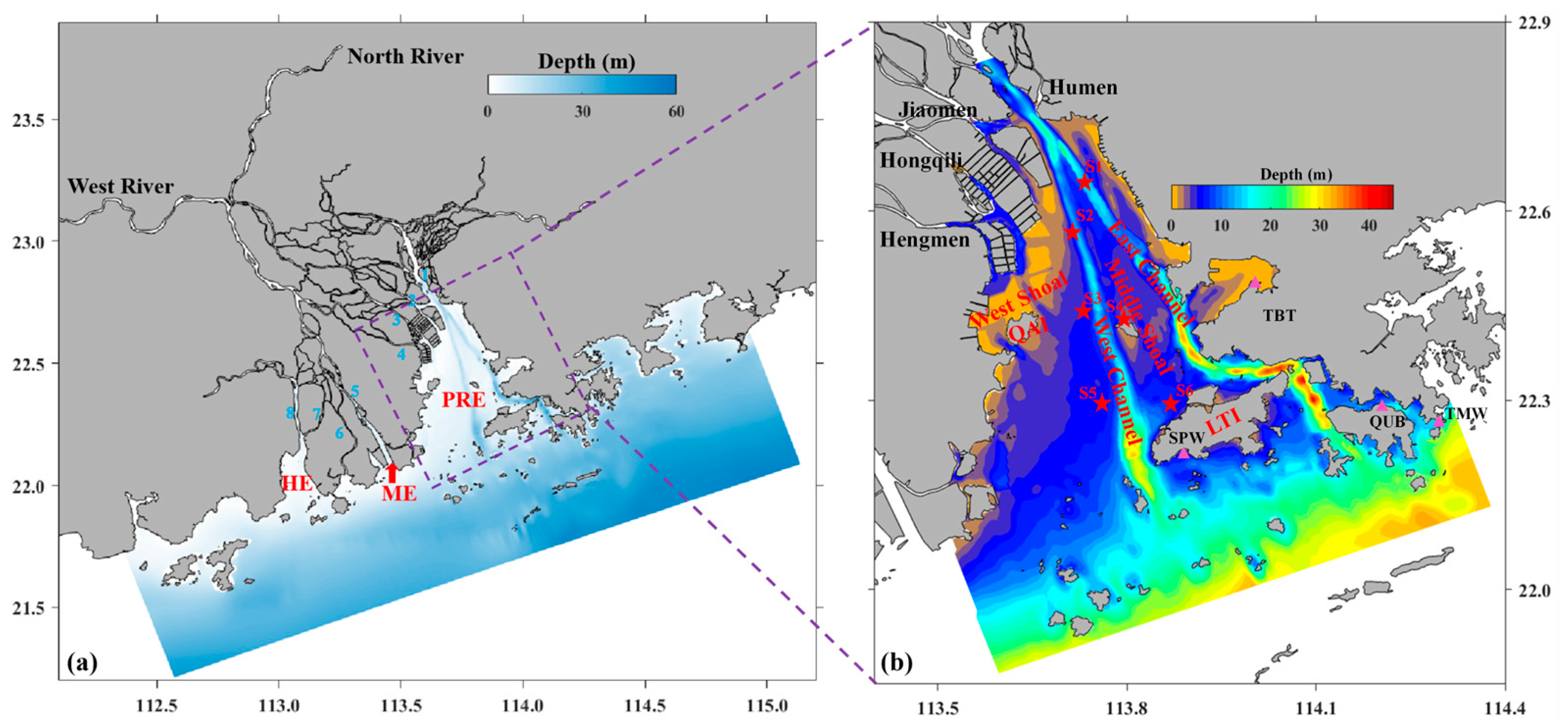
2. Regional Settings

The Pearl River Delta, situated in South China, originates from the Pearl River and extends to the northern shelf of the South China Sea (Figure 1a). This delta receives an annual freshwater influx of 2.86 × 10¹¹ m³ from the three principal tributaries of the Pearl River: the West River, North River, and East River. The Pearl River Delta features eight outlets from east to west: Humen, Jiaomen, Hongqili, Hengmen, Modaomen, Jitimen, Hutiaomen, and Yamen. Approximately 63.5% of the river’s runoff discharges into the Pearl River Estuary (PRE) through the four eastern outlets (Figure 1b). The axial length of the PRE extends about 70 km from its head near the Humen outlet to the estuary mouth between Macau and Hong Kong. The topography of the PRE is funnel-shaped, with a width of approximately 40 km at its mouth, tapering to 6 km at the Humen outlet. The estuary encompasses an area of around 1900 km² and is characterized by two channels (the West Channel and the East Channel) and three shoals (the West, Middle, and East Shoals). Depths range from 2.0 m on the shoals to 30 m in the deep channels.

The PRE exhibits a micro-tidal regime, with tidal ranges spanning from 1.0 to 1.7 m, propagating from the estuary mouth to its head. The predominant tidal constituent is M₂, followed by K₁ and O₁ constituents [23]. The interaction between tidal currents and the intricate bathymetry induces considerable spatial variation in stratification within the estuary. The PRE is subject to a monsoon climate, resulting in pronounced seasonal variations in wind forcing and river discharge between summer and winter. During the summer, river discharge is substantial, accounting for 80% of the annual runoff, and is accompanied by mild southwesterly winds. In contrast, the winter season is characterized by low river discharge and strong northeasterly winds. Due to the wide basin and the influence of the northeasterly winds, the outflow tends to remain adjacent to the West Shoal [20]. In this study, we will employ numerical models to investigate the impacts of wind on estuarine hydrodynamics and stratification processes.

3. Methods

3.1. Numerical Model

In this study, we utilized the Environmental Fluid Dynamics Code (EFDC), a modeling tool renowned for its successful application across diverse aquatic environments, encompassing estuaries, rivers, lakes, and lagoons [24,25,26]. Analogous to the widely acclaimed Princeton Ocean Model [27], EFDC employs robust physical formulations and computational schemes. It rigorously solves the three-dimensional continuity and Navier-Stokes equations within a specified domain under the hydrostatic assumption and Boussinesq approximation. The model employs curvilinear, orthogonal horizontal coordinates and sigma vertical coordinates. EFDC integrates the modified Mellor-Yamada level 2.5 turbulence closure [28,29] to compute turbulent viscosity and diffusivity. Furthermore, it incorporates a wet/dry scheme developed by Hamrick [30] to precisely simulate hydrodynamics in shallow areas. Capable of capturing dynamics influenced by density gradients, topography, tides, and wind forcing, EFDC models the transport of salinity, temperature, and both conservative and non-conservative tracers with fidelity.

3.2. Model Setup

A hierarchical nesting-domain strategy was employed to dynamically connect a comprehensive model of the Pearl River Delta with a finely resolved model of the Pearl River Estuary (PRE), as illustrated in Figure 1. The expansive domain model accounts for frequent water exchanges between the PRE and adjacent coastal seas, offering boundary conditions for the high-resolution sub-model. This strategic approach not only enhances computational efficiency but also integrates coastal dynamic processes seamlessly. Detailed implementation and validation of the large-domain model are documented in Zhang et al. [31]. The sub-model encompasses the region from the four tributaries extending to offshore areas, where water depths reach approximately 30 m (Figure 1b). Configured with 378 × 295 horizontal grid cells, the sub-model achieves resolutions ranging from 150 m within the estuaries to about 800 m at the open sea boundary. High-resolution grid cells are strategically positioned in the deep channels to accurately depict the intricate geometry of the PRE. Vertical discretization comprises sixteen water column layers using sigma coordinates, with finer resolutions near the surface and bottom to meticulously resolve boundary layers. The wetting-drying method is employed to improve simulation accuracy on shallow shoals. Hydrodynamic roughness coefficients, calibrated during model development, vary between 0.002 and 0.005 m. The temperature simulation incorporates atmospheric pressure, temperature, solar shortwave radiation, relative humidity, evaporation, precipitation, and cloud cover data to establish the temperature module [30].

Initial and boundary conditions for tidal elevation, tidal current, salinity, and river discharge were derived from a pre-existing large-domain model that encompasses the inner shelf, the estuary, and the upstream river networks [31]. Given that the initial salinity and velocity of the model were interpolated from the large-domain model outputs, the hydrodynamic spin-up was minimal and did not impact the estuarine dynamics.

In this study, we use the buoyancy frequency to evaluate the variation in stratification.

$$N^2=-{\displaystyle \frac{g}{{\rho }_0}}{\displaystyle \frac{\partial \rho }{\partial z}}$$

(1)

where $N$ is the buoyancy frequency, ${\rho }_0$ is the reference density, g denotes the gravitational constant, and $\rho$ denotes the density in each water column layer. To discern the impacts of tidal and wind forces on density stratification, two model scenarios were conducted. In Case 1, the model was driven by river discharge from the upstream river network and tides at the open sea boundary, with river discharge varying between 2800 and 12,000 m³/s during the simulation period (Figure 2a). Due to the substantial freshwater discharge in the latter part of the simulation, only the first half of the results was utilized to investigate stratification variation, thereby representing typical buoyancy input in the PRE during dry seasons. In Case 2, wind forcing was incorporated into the model. Wind data were obtained from the Climate Forecast System Reanalysis (National Centers for Environmental Prediction) with a temporal resolution of 6 h and a spatial resolution of 0.3 × 0.3°. During the simulation, a prevailing northeasterly wind was observed (Figure 2c), characteristic of the dry season. By comparing the results from these two scenarios, we can effectively analyze the hydrodynamic changes induced by wind forcing during the dry season and its subsequent impacts on density stratification. The model setup, including the data sources, is summarized in

Table 1. Summary of numerical experiments. The “×” symbols indicate that wind forcing is excluded for a specific model case.

Model Cases	River Discharge	Tidal Elevation	Wind
Case 1	3800~12,000 m3/s, daily measured data in upstream tributaries	The tidal range varies from 0.68 to 2.70 m, driven by 11 harmonic tidal constituents extracted from [31].	×
Case 2			Averaged wind: 6.9 m/s with a direction of 248°, obtained from the Climate Forecast System Reanalysis (NCEP, https://climatedataguide.ucar.edu/climate-data/climate-forecast-system-reanalysis-cfsr (accessed on 12 June 2021))

.

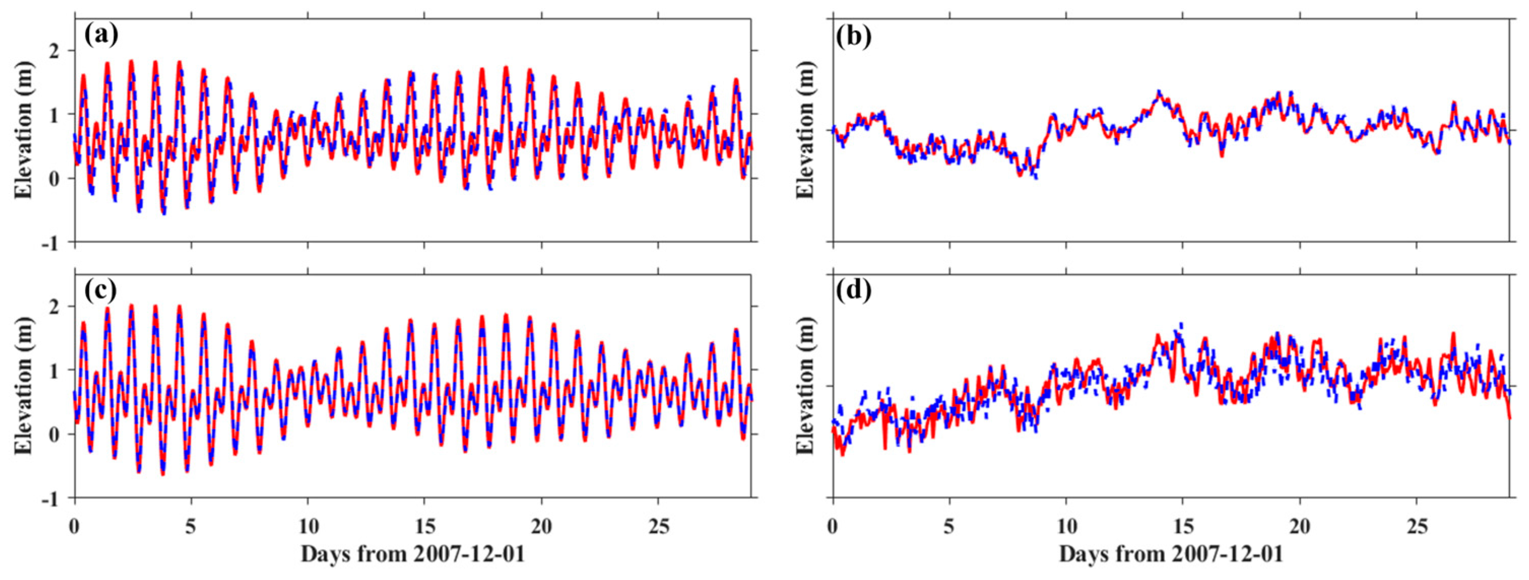
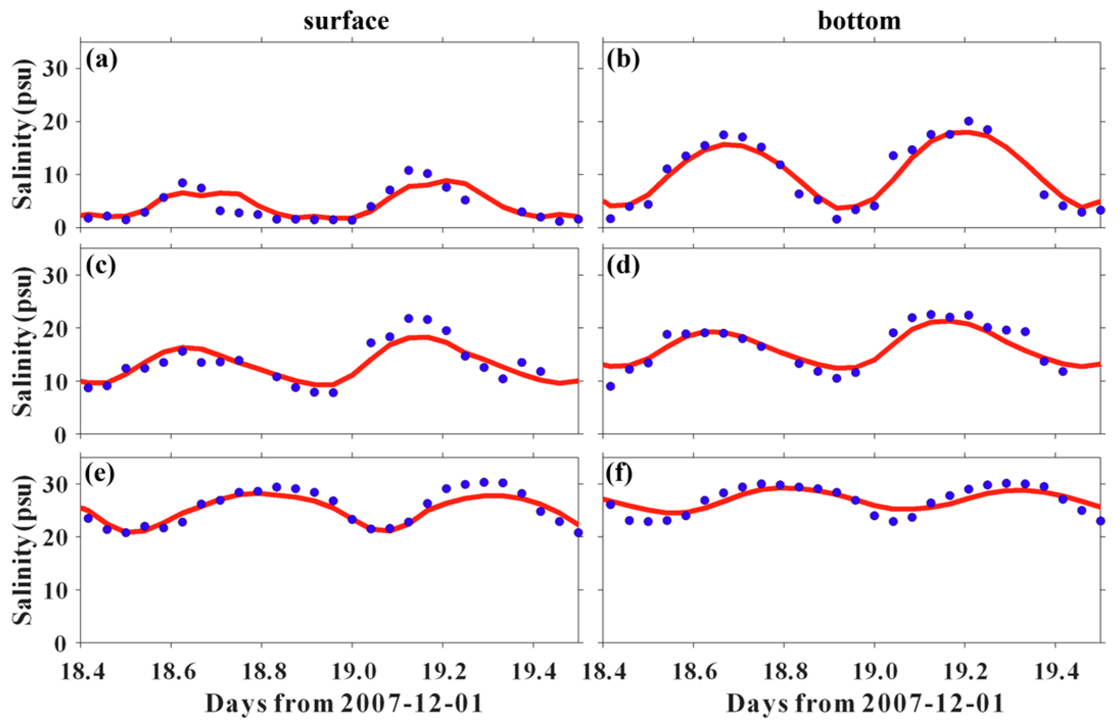
3.3. Model Calibration

To evaluate the model’s performance, the simulated tide was compared with observed water levels from December 2007. Due to freshwater input and prevailing winds, the water level can exhibit non-tidal signals. Therefore, we also examined the residual water level by excluding tidal-induced variations. For calibration of the tidal current and salinity, in-situ measurements from surveys conducted during the winter of 2007 were utilized. These measurements were taken during a spring tide, with tidal current and salinity continuously recorded for approximately 27 h. To quantitatively assess the model’s accuracy, its performance was evaluated using the skill score (SS) [32].

$$SS=1-{\displaystyle \frac{\sum _{i=1}^N(m_i-o_i{)}^2}{\sum _{i=1}^N[\left|m_i-\overline{o}\right|+\left|o_i-\overline{o}\right|{]}^2}}$$

(2)

where $\overline{o}$ is the mean value of observations. The SS is a measure of the agreement between the model results and observations, with a SS value of 1 indicating perfect agreement and a value of 0 indicating complete disagreement.

The water levels were calibrated by adjusting the bottom roughness height to ensure the simulated levels closely matched the observed values. The comparison of water levels at the QUB and SPW stations (refer to Figure 1b for locations) is shown in Figure 3. The simulated water levels exhibit strong consistency with the observations, particularly during the spring tide. The SS for water level are 0.95 and 0.94 at the selected stations, indicating excellent model performance. For the dominant M₂ tidal constituent, the mean error for amplitude is less than 4%, and the mean phase difference is less than 8%. The variations in non-tidal water levels are more complex due to the intricate bathymetry, river discharge, and wind effects. Consequently, the SS values for non-tidal water levels are 0.86 and 0.74, which, although slightly lower than those for tidal water levels, still demonstrate acceptable performance. Overall, the water level simulations are satisfactory.

Comparisons of tidal current and salinity between simulated results and measurements at three selected stations are presented in Figure 4 and Figure 5, respectively. The modeled current speed and direction closely follow the observed data, with values of SS for tidal current ranging from 0.55 to 0.68, indicating very good to excellent performance. The simulated current speed at the surface layer is slightly lower than the observed values, likely due to the model grid resolution, which may not be fine enough to capture small-scale topographical changes accurately. The modeled salinity fluctuations and vertical stratification align well with the observed values. Discrepancies mainly occur during peak floods and ebb tides, consistent with the underestimated tidal currents. The SS values for salinity range from 0.61 to 0.83, signifying excellent performance. Overall, the model effectively captures the tidal dynamics and salinity transport in the PRE, making it a reliable tool for diagnosing the stratification processes of the estuary.

4. Results

4.1. Water Exchage

Density stratification in estuaries is primarily governed by the interplay between freshwater inflows and saline intrusions. To elucidate this process, we first examine the subtidal salinity and residual currents in the PRE. During neap tide, the subtidal current near the estuary head at the Humen Outlet flows downstream, driven by the high inertia of freshwater (Figure 6a). Freshwater from the lateral tributaries establishes an eastward barotropic pressure gradient, generating a robust lateral current in the upper reaches of the West Shoal. Due to the unique geometry of the PRE, saline water tends to intrude along the deep channels, creating a transverse salinity gradient between the West Shoal and the West Channel. This gradient acts as a dynamic barrier, preventing freshwater from the lateral tributaries from spreading further eastward within the estuary [33]. In the lower reach of the estuary, the subtidal current veers southwest, transporting freshwater to the West Shoal and the eastern portion of the West Channel. Concurrently, high-salinity water intrudes from the eastern part of the estuary, consistent with observations in other dynamically wide estuaries [34,35]. In the eastern part of the estuary, the landward subtidal current is attenuated due to strong tidal mixing, resulting in reduced landward salinity transport during spring tide (Figure 6b). This modification in salinity structure diminishes the transverse density gradient, enabling freshwater from the lateral tributaries to spread further eastward during spring tide.

The simulation results of Case 2 reveal that seaward freshwater transport is significantly enhanced during both neap and spring tides under the influence of northeasterly winds (Figure 3c,d). The intrusion of high-salinity water extends further upstream in the eastern part of the estuary, with the 30-psu salinity isoline advancing approximately 12 km upstream compared to Case 1. In the transition zone between the West Shoal and the West Channel, the lateral component of the current is intensified, thereby constraining the freshwater to a narrower region. Consequently, the subtidal current is augmented, and a pronounced transverse salinity gradient is established.

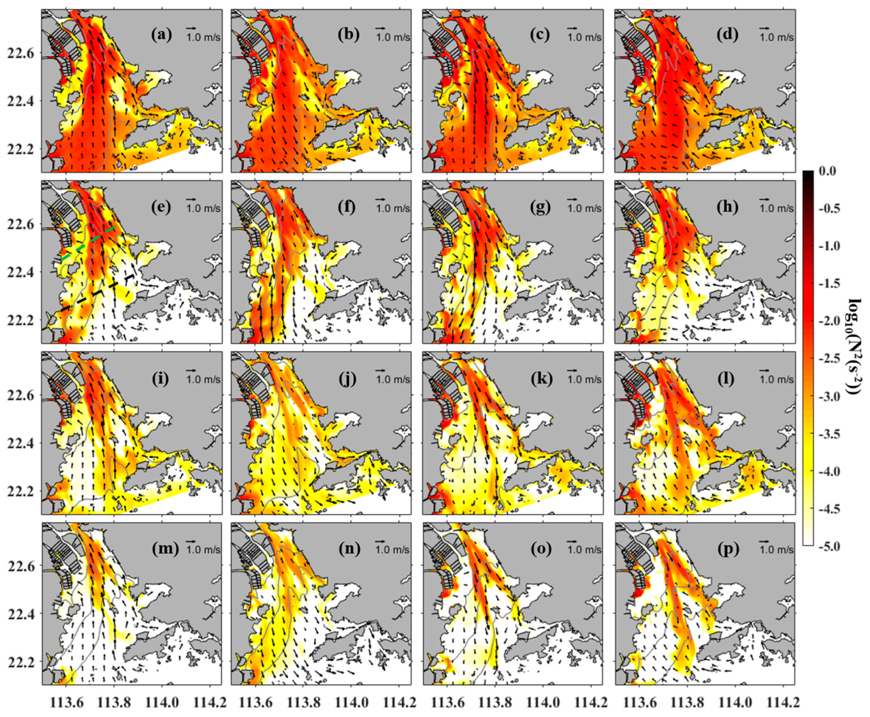
4.2. Intra-Tidal Variation in Stratification

Density stratification in the PRE exhibits marked spatial and temporal variations due to its complex bathymetry and hydrodynamic conditions. In the simulation without wind, the water column remains stratified in the West Channel throughout the neap tide (Figure 7a–d), with squared buoyancy frequency values exceeding 10⁻² s⁻². In the upper estuary, the water column is most stratified during ebb slack, highlighting the significant role of longitudinal straining in modulating stratification. In the lower estuary, the spatial distribution of squared buoyancy frequency corresponds with the freshwater spreading pattern. Buoyancy input from upstream, interacting with denser water, leads to vigorous stratification in the western part of the estuary. On intra-tidal timescales, density stratification develops in the lower estuary when lateral flow intensifies, such as during flood slack and ebb slack (Figure 7b–d). This indicates that the mechanisms controlling stratification in the lower estuary differ from those in the upper reach, a topic we will discuss further. Due to relatively smaller buoyancy input, the water column in the East Channel is less stratified, with squared buoyancy frequency values ranging between 10⁻⁴ and 10⁻³ s⁻². During the spring tide, density stratification is disrupted by the energetic tidal currents (Figure 7i–l). Apparent stratification is observed only in the deep channels, where freshwater and high-salinity water converge. Conversely, on the shallow shoals, the squared buoyancy frequency decreases to less than 10⁻⁵ s⁻² for most of the flood-ebb cycle. However, during flood slack, the squared buoyancy frequency increases to 10⁻⁴ s⁻² when the lateral flow is vigorous.

The density stratification in the PRE is influenced by northeasterly winds during both the neap tide (Figure 7e–h) and the spring tide (Figure 7m–p). The wind stress alters the spatial distribution pattern of stratification by modifying the seaward transport of freshwater. In the upper estuary during the neap tide, stratified water accumulates in the deep channels. As the estuary widens downstream, low-salinity water turns southwestward, gathering in the lower part of the West Shoal. In the lower estuary, the deep channels are predominantly filled with high-salinity water, resulting in a well-mixed water column with squared buoyancy frequency values less than 10⁻⁵ s⁻². Conversely, the water mass on the West Shoal retains some stratification due to the density contrast between freshwater and saline water. Throughout a flood-ebb tidal cycle, the West Shoal exhibits the highest level of stratification during the flood slack (Figure 7f), suggesting that lateral straining may be pivotal in stratification when a pronounced transverse salinity gradient exists [9]. During the spring tide, stratification diminishes further under the combined influence of wind stress and vigorous tidal mixing. In the upper estuary, density stratification is more pronounced during the ebb tide compared to the flood tide. In the lower estuary, stratification is most evident at the boundary between deep channels and shoals. Moreover, the West Shoal remains slightly stratified, displaying notable intra-tidal variations that peak notably during the flood slack, akin to the situation during the neap tide.

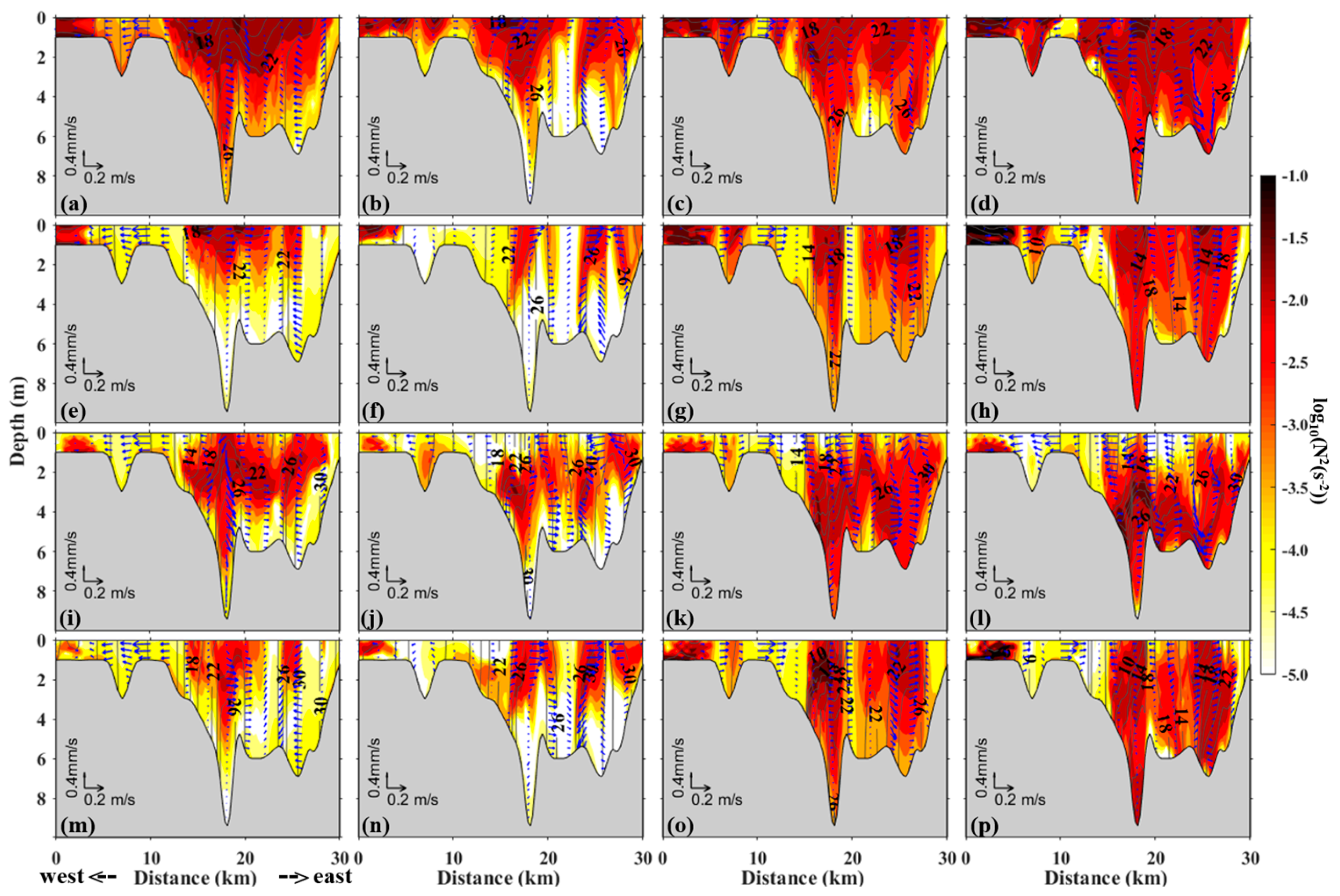
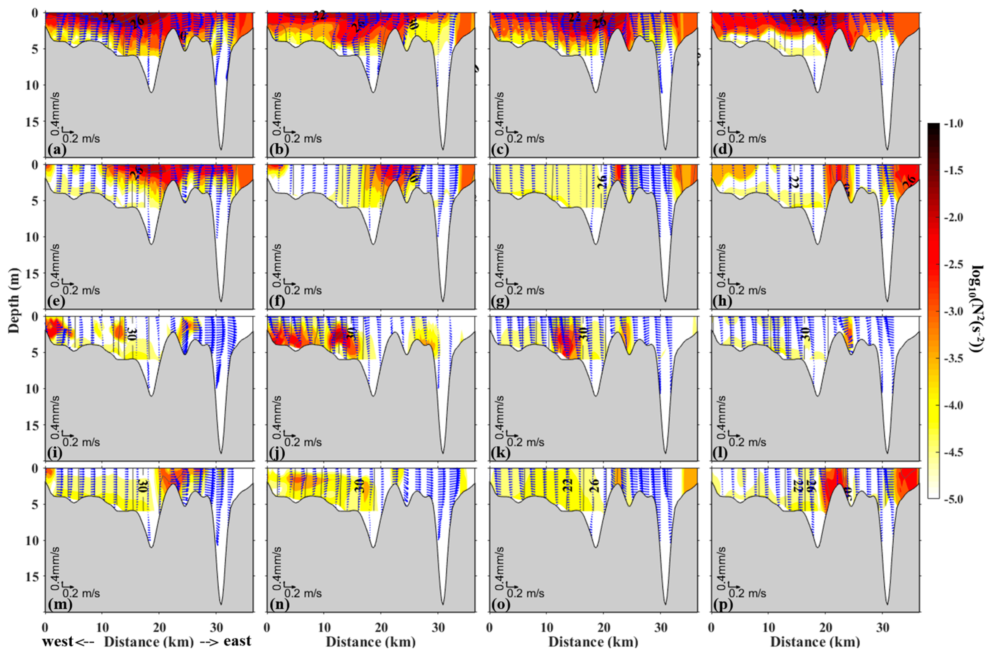
4.3. Transverse Distribution of Stratification

Here, we present the transverse structure of salinity, tidal current, and buoyancy frequency to further investigate the detailed mechanisms of stratification. Two transects were selected (one in the upper estuary and the other near the mouth; see Figure 7e for locations) to illustrate how salinity and associated stratification are modulated by transverse variations in bathymetry. In the upper transect, the upper water column in the deep channel is more stratified than other parts of the transverse section. Due to the weak currents during the neap tide, there is a persistently strong vertical salinity gradient in the upper 6 m of the water column in the deep channel (Figure 8a–d). Under the influence of friction, the salinity profile exhibits a well-mixed state near the bottom during the flood tide. The vertical shear of the ebb current strains the isopycnals, resulting in an increased vertical salinity gradient in the lower water column. The density stratification exhibits a similar spatial and temporal pattern to the vertical salinity gradient. Lateral flows in the upper transverse section have a minor impact on the evolution of density stratification for most of the flood-ebb cycle. However, during the late period of the flood tide, the lateral current shear strains the isopycnals, leading to a strong vertical salinity gradient in the surface layer of the West Channel (Figure 8b). During the spring tide, the salinity profile is vertically uniform on the shallow shoal during the flood tide (Figure 8e,f). In the eastern part of the transect, a strong vertical salinity gradient appears only in the surface layer and decreases rapidly toward the lower water column due to vigorous turbulence produced by the interaction between tidal currents and the seabed. Similar to the neap tide, stratification is enhanced during the ebb phase of the tidal cycle (Figure 8g,h). The magnitude of lateral flows decreases during the ebb tide, rendering its impact on stratification negligible.

The influence of wind stress on salinity transport manifests in increased salinity within the channels and decreased salinity on the shallow shoals during both neap and spring tides (Figure 8i–p). Additionally, the vertical salinity profile undergoes modifications due to direct mixing effects. On the shallow shoals, wind-induced mixing permeates the entire water column, resulting in a minimal vertical salinity gradient. However, in the deep channels, the impact of wind stress on stratification varies between neap and spring tides. During neap tides, wind mixing primarily affects the surface layer (Figure 8i–l). Below the surface mixed layer, density stratification demonstrates a pattern of increasing followed by decreasing buoyancy frequency due to intensified mixing near the seabed. The northeasterly wind induces persistent westward lateral flow near the surface, while the current in the middle and bottom layers predominantly flows eastward. Strong lateral current shear occurs in regions coinciding with vigorous stratification. During spring tides, the combined effects of wind and tidal mixing further diminish stratification (Figure 8m–p), particularly noticeable during the flood tide, where squared buoyancy frequency values typically fall below 10⁻³ s⁻².

The dynamics in the lower transect undergo significant transformations, exerting a distinct influence on density stratification. A persistent and robust transverse salinity gradient is evident along the periphery of the West Shoal during neap tides (Figure 9a–d), corresponding with the area of outflow (Figure 6a). Vertically, pronounced lateral current shear is observed within the pycnocline. The interplay between lateral current shear and the transverse salinity gradient results in vigorous stratification on the West Shoal and the western segment of the West Channel. Conversely, the eastern part of the estuary exhibits minimal salinity gradients in both transverse and vertical dimensions. During spring tides, the water column over the West Shoal displays a well-mixed state due to intensified mixing (Figure 9e–h). Meanwhile, currents in the Middle and East Shoals are relatively weak, resulting in corresponding stratification patterns.

Under the influence of the prevailing northeasterly wind, stratification undergoes attenuation during both neap and spring tides (Figure 9i–p). The wind stress directly mixes the surface layer, causing the region of pronounced stratification to descend into the middle and lower layers. Furthermore, the wind intensifies both the seaward outflow and the landward inflow (Figure 6c,d). Spatially, the outflow is confined to a narrower area in the West Shoal, creating a robust lateral salinity gradient. Particularly noteworthy is the differential advection during the spring tide, as highlighted by Zhu et al. [10], which also induces a pronounced lateral salinity gradient between the West Channel and Middle Shoal (Figure 9o,p). This interaction with the lateral current shear is anticipated to foster strong stratification within these regions.

5. Discussion

5.1. Wind Modulation on Water Transport

The results reveal that wind forcing restricts upstream freshwater from dispersing widely within the estuary, concentrating it close to the estuary’s right bank, while salinity rises in the eastern sector. In shallow estuaries, stratification arises from the density contrast created by freshwater inflow and saline water intrusion [36]. To deepen our comprehension of how winds influence the salinity distribution, we analyzed the water flux. Rather than mapping freshwater and saltwater fluxes directly, we illustrate the water flux within a salinity-distance framework [37,38].

$$Q\left(s,x\right)=<{\int }_{A_s}udA>$$

(3)

where $A_s$ is the cross-sectional area with salinity greater than $s$, $u$ is the longitudinal current velocity, the flux is calculated along the estuary with coordinate x (originating from the estuary mouth), and brackets denote a tidally averaged (a 15-day filter) value. In this study, a positive flux denotes landward water transport, and a negative value denotes seaward flow.

The results of isohaline flux are depicted in Figure 10. In Case 1, water movement seaward is evident across all salinity bands between distances of 60–70 km, indicating a lack of landward subtidal flow near the estuary head. Following freshwater input from lateral tributaries into the PRE, seaward water flux increases to 3000 m³/s. Concurrently, a modest landward flux is observed within salinity bands ranging from 10 to 18 psu, illustrating a typical exchange flow structure within the estuary [39]. Downstream, seaward flow remains consistently constrained within the low-salinity band due to plume dispersion. In the lower estuary, intensified estuarine circulation leads to an increased landward water flux. Under the influence of northeasterly winds (Case 2), distinct effects are observed along the PRE. In the upper estuary, seaward flux appears in similar salinity bands as in the absence of wind. However, wind-induced salinity intrusion intensifies, accompanied by a noticeable landward flux. Downstream, seaward flux occurs in lower salinity bands as the outflow extends further westward. Conversely, landward flux is observed in higher salinity bands, creating a strong lateral salinity gradient between seaward outflow and landward inflow. Vertical shear within lateral currents, induced by wind stress, promotes lateral straining, thereby contributing to density stratification (Figure 7i–p).

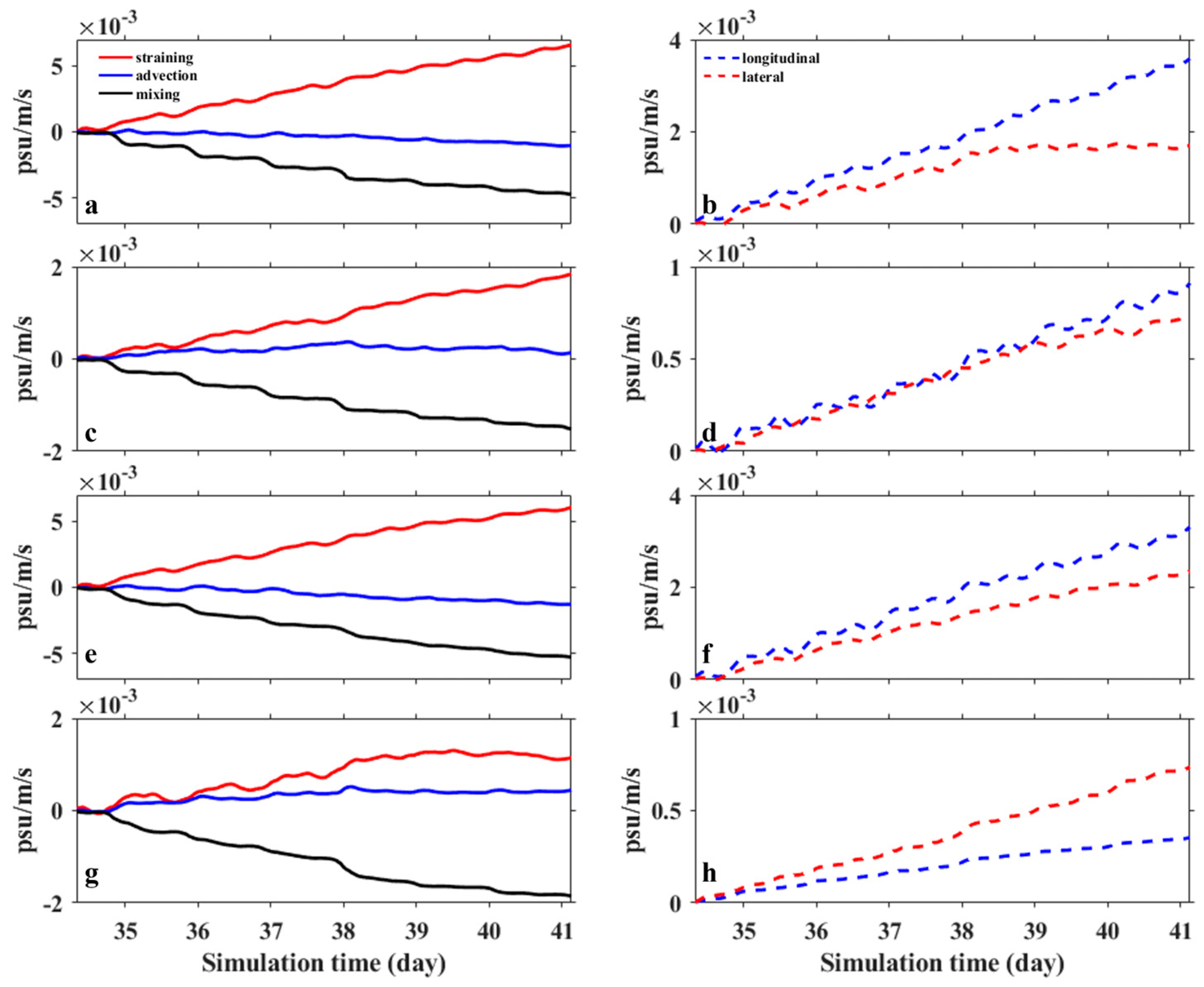
5.2. Controlling Factors in Stratification

The results reveal distinct disparities in both the spatial distribution and variability of density stratification between the upper and lower estuaries. Previous investigations have elucidated how tidal straining, advection, and vertical mixing can modify stratification [40]. Alterations in hydrodynamics have the potential to influence these processes, thereby impacting both stratification and destratification dynamics. Here, we scrutinize the evolution of vertical salinity gradients as pivotal factors governing stratification:

$${\displaystyle \frac{\partial }{\partial t}}{\displaystyle \frac{\partial s}{\partial z}}=-\stackrel{straining}{\overbrace{({\displaystyle \frac{\partial u}{\partial z}}{\displaystyle \frac{\partial s}{\partial x}}+{\displaystyle \frac{\partial v}{\partial z}}{\displaystyle \frac{\partial s}{\partial y}})}-}\stackrel{advection}{\overbrace{(u{\displaystyle \frac{\partial }{\partial x}}{\displaystyle \frac{\partial s}{\partial z}}+v{\displaystyle \frac{\partial }{\partial y}}{\displaystyle \frac{\partial s}{\partial z}})}}+\stackrel{mixing}{\overbrace{{\displaystyle \frac{\partial }{\partial z}}{K}_v\left({\displaystyle \frac{{\partial }^{2}s}{\partial z^2}}\right)}}$$

(4)

where $K_v$ is the eddy diffusivity, $v$ is the lateral velocity. In this equation, the term on the left side is the rate of change in the vertical salinity gradient; the first two terms on the right-hand side are the straining terms, which can be further decomposed to the longitudinal (${\displaystyle \frac{\partial u}{\partial z}}{\displaystyle \frac{\partial s}{\partial x}}$) and lateral (${\displaystyle \frac{\partial v}{\partial z}}{\displaystyle \frac{\partial s}{\partial y}}$) straining, the next two terms represent advection, which can be further decomposed to the longitudinal ($u{\displaystyle \frac{\partial }{\partial x}}{\displaystyle \frac{\partial s}{\partial z}}$) and lateral ($v{\displaystyle \frac{\partial }{\partial y}}{\displaystyle \frac{\partial s}{\partial z}}$) advection; and the last term denotes the vertical mixing. The remaining terms, including vertical advection, vertical straining, and horizontal mixing, are omitted in this equation since they have relatively smaller effects on density stratification [10,15]. In this study, we integrated the equation over the selected transects to examine time series change in these terms:

$$\overline{\mathsf{\varphi }}={\displaystyle \frac{{\int }_A\varphi dA}{{\int }_{A}dA}}$$

(5)

where $\varphi$ denotes either term on the right side of Equation (3), A is the area of the selected transects, and the overbar denotes the transversely averaged value. The values of the area-averaged term are further integrated over time to examine the overall impacts on stratification.

$$[\overline{\mathsf{\varphi }}]={\int }_0^T\overline{\varphi }dt$$

(6)

where the square bracket denotes the integration values over time (from the beginning of spring tide to the end of neap tide).

In the upper transect (marked by the green dashed line in Figure 7e), stratification was influenced by tidal straining and vertical mixing when excluding wind effects (Figure 11a). The contribution from integrated advection terms was relatively minor, indicating a negligible impact on stratification. Longitudinal straining was predominant, with a value of 3.3 × 10⁻³ psu/m/s, while lateral straining contributed 2.1 × 10⁻³ psu/m/s (Figure 11b), underscoring the dominant role of longitudinal straining in modifying stratification. During flood tide, longitudinal straining acted to destratify the water column, whereas it enhanced density stratification during ebb tide (Figure 8a–d). Vertical mixing displayed a phase variation aligned with longitudinal straining, generally attenuating stratification, as posited by Burchard and Hofmeister [41]. Similarly, in the lower transect (refer to the black dashed line in Figure 7e), stratification without wind was governed by straining and mixing terms. However, these terms exhibited a declining trend overall (Figure 11c). Longitudinal and lateral straining terms were comparable in magnitude (Figure 11d), emphasizing the significance of interactions between vertical shear in lateral currents and transverse salinity gradients in modulating stratification. In the outflow region of the lower transect, lateral current shear strained isopycnals, resulting in apparent stratification there (Figure 9a–d).

Under the influence of wind forcing, there is a notable increase in vertical mixing in the upper transect (Figure 11e), indicating that wind stress imparts energy to the water column, facilitating mixing. Conversely, the straining value decreases in the upper estuary. These alterations in vertical mixing and straining contribute to a reduction in stratification (Figure 8e–h). Specifically, there is a declining trend in longitudinal straining, while integrated lateral straining increases to 2.3 × 10⁻³ psu/m/s. The rise in lateral straining is closely associated with changes in circulation patterns and the salinity distribution. With wind included, a transversely sheared estuarine circulation emerges freshwater moves seaward in the western part of the estuary, while saline water is constrained in the deep channels on the eastern side [17]. Consequently, a strong lateral salinity gradient develops. Moreover, wind induces vigorous lateral currents near the surface layer, augmenting shear in the lateral current. This interaction between lateral current shear and the transverse salinity gradient fosters pronounced lateral straining and stratification in the transitional zone between the West Shoal and West Channel, where intense stratification occurs. In the lower transect, vertical mixing increases further due to the northeasterly wind (Figure 11g), leading to reduced stratification compared to the upper transect (Figure 8 and Figure 9). Influenced by the widened estuary and the northeasterly wind, lateral currents predominantly flow westward over the West Shoal during most of the tidal cycle (Figure 9i–p). Consequently, stratified water is transported by the lateral current to the westernmost part of the estuary, underscoring the importance of advection in modifying stratification. Similar to the upper estuary, the transverse flow structure creates a significant lateral salinity gradient, thereby enhancing lateral straining (Figure 11h).

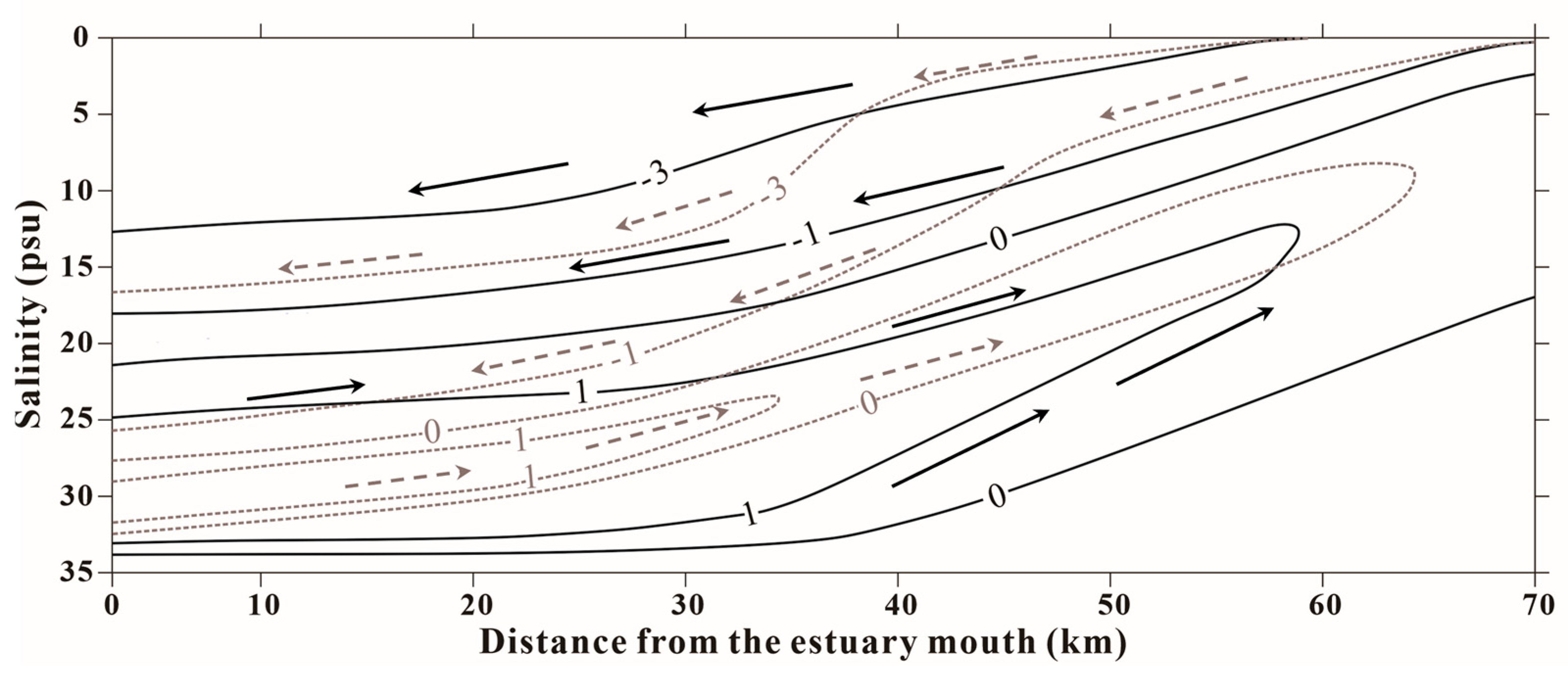
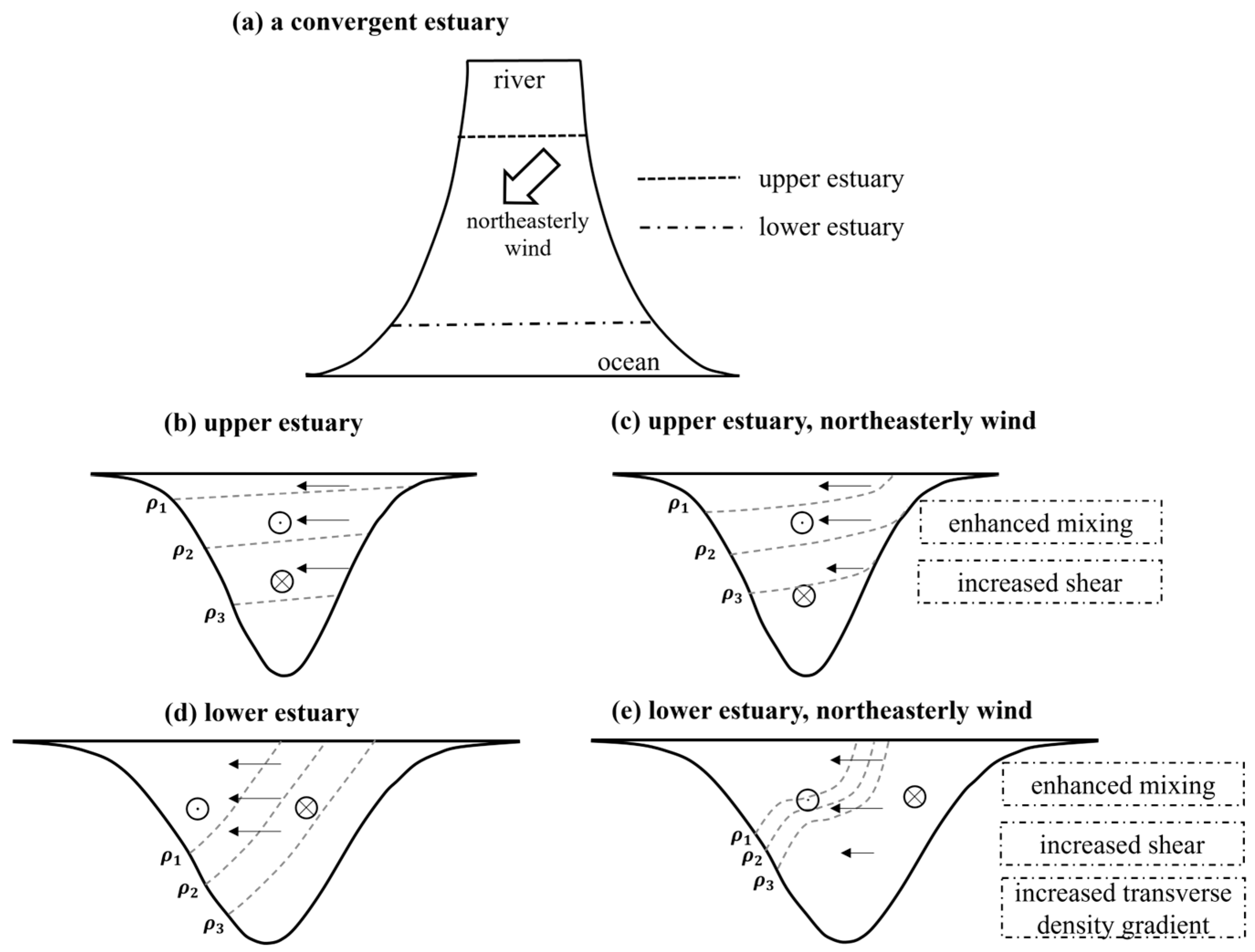
5.3. Conceptual Diagram and Comparisons with Other Estuaries

Previous studies have underscored the significance of basin width in shaping estuarine hydrodynamics [15,34]. Consistent with these findings, our research demonstrates that stratification processes are intricately linked to variations in estuary width. We present a conceptual diagram elucidating how stratification responds to wind forcing and estuary width in a convergent estuary, where the width expands seaward (Figure 12a). During our simulations, the Kelvin number in the upper estuary is approximately 0.89, indicating that the Coriolis force exerts a minimal influence on modulating the exchange flow pattern due to the relatively narrow width of the estuary. In this scenario, landward inflow is constrained near the bottom, while seaward outflow predominates in the surface layer (Figure 12b). Correspondingly, the isopycnal surfaces are nearly flattened near the surface, resulting in a low transverse density gradient. With weak lateral flow shear, the impact of lateral straining on modulating the density gradient is negligible. Wind-induced mixing tilts the isopycnals near the surface (Figure 12c), leading to a reduction in the density gradient. Under this mixed surface layer, enhanced lateral flow induces strong shear. The vertical shear in lateral flow further strains the isopycnals, contributing to a slight increase in lateral straining (Figure 11f). However, the magnitude of lateral straining remains limited due to the weak transverse density gradient. Therefore, in the upper estuary, stratification is primarily governed by longitudinal straining under both model scenarios, with and without the influence of northeasterly wind.

In the lower estuary, the Kelvin number increases to 9.67. Influenced by the Coriolis force, the outflow veers left and concentrates in the western part of the estuary, while the landward inflow is confined to the right side [34]. Consequently, a transversely sheared exchange flow structure emerges in the lower estuary (Figure 12d). The density difference between the inflow and outflow establishes a prominent transverse density gradient. Interacting with the lateral flow shear, lateral straining becomes significant in modulating stratification, achieving a magnitude comparable to longitudinal straining (Figure 11d). The northeasterly wind intensifies estuarine circulation, leading to an increase in the transverse density gradient (Figure 12e). Wind forcing also enhances lateral flow shear, further increasing lateral flow, which becomes dominant in modulating density stratification. Stratification is most pronounced at the interface between inflow and outflow, where the largest transverse density gradient occurs. Similar to the upper estuary, wind-induced mixing weakens density stratification in the upper water column.

Wind significantly influences salinity transport, which in turn affects density stratification. Averaged over tidal cycles, a down-estuary wind tends to intensify the seaward transport of salinity at the surface layer and the landward transport of salinity near the bottom. This enhances stratification by increasing the vertical salinity gradient [14]. Conversely, an up-estuary wind can reduce the two-layer salinity transport, resulting in decreased stratification [13]. Compared to a long-estuary winds, cross-estuary winds have a minor impact on stratification [41]. This relationship between wind forcing and stratification alteration is particularly evident in narrow estuaries where the transverse salinity gradient is low, such as the York River Estuary, Ringkøbing Fjord, and the Magdalena River estuary.

The wind plays a key role in modulating salinity transport, which consequently alters the density stratification. In the tidal-average sense, a down-estuary wind tends to intensify seaward salinity transport at the surface layer and landward salinity transport near the bottom, which enhances the stratification by increasing the vertical salinity gradient [14]. By contrast, an up-estuary can reduce the two-layer salinity transport and result in a decrease in stratification [13]. Compared to the along-estuary wind, the cross-estuary wind has a minor impact on stratification [42]. These correspondences between wind forcing and alteration in stratification are valid in narrow estuaries owing to the low transverse salinity gradient, such as the York River Estuary [43] and the Ringkøbing Fjord [44]. As illustrated in Figure 12, wide estuaries with a high Kelvin number often exhibit transversely sheared estuarine circulation, with seaward outflow on one side and landward inflow on the other [17]. Consistent with this circulation pattern, freshwater exits the estuary through the outflow, while saltwater intrudes on the opposite side. For example, in the South Passage of the Changjiang Estuary, a significant number of freshwater veers rightward at the mouth, while saline water moves landward in the northern part of the channel [45,46]. This creates a pronounced transverse gradient, making lateral straining crucial in modulating stratification. Under the influence of northeasterly winds, the outflow is intensified, and density stratification primarily occurs at the interface between the seaward-transported freshwater and the landward saline water. Moreover, wide estuaries often feature one or several channel-shoal systems. Regions with high transverse salinity gradients can also be observed at the channel-shoal interfaces (e.g., the West Channel-Middle Shoal interface and the East Channel-East Shoal interface in the PRE), where strong stratification can be promoted.

In this study, we examined the impact of northeasterly winds on stratification in the wide PRE without exploring the full parameter space of variations in wind direction and estuary width. Consequently, we did not present a quantitative relationship between wind forcing and density stratification. Nevertheless, our findings have significant implications for other wide estuaries, such as the Chesapeake Bay [47] and the Delaware Bay [18,35], where a transversely sheared structure of estuarine circulation is observed. Furthermore, the numerical model employed in this study, which accounts for continuous vertical variation and temporal evolution in density within a specific estuary, demands substantial computational resources. This constraint makes it challenging to conduct numerical experiments that consider the full range of wind speeds, directions, tidal ranges, and estuarine convergence. Future research should employ models based on analytical methods [48] or depth-integrated, multi-layer approaches [49], which offer greater computational efficiency. These models can be utilized to obtain in-depth knowledge about stratification and estuarine circulation under complex driving forces in estuaries.

6. Conclusions

In this investigation, we utilized the EFDC model to explore changes in estuarine circulation and their impact on density stratification in the PRE. We compared scenarios without wind and under prevailing northeasterly winds during the dry season. Our analysis delves into the mechanisms governing the stratification process by examining the evolution of the vertical salinity gradient. Our findings reveal that in the upper estuary, density stratification is primarily influenced by longitudinal straining. This process intensifies stratification during ebb tide while diminishing it during flood tide. As the estuary widens in its lower reaches, characterized by a Kelvin number near 10, freshwater from the headwaters flows toward the estuary’s right side, while high-salinity water penetrates inland through the eastern sector. This spatial water mass transport establishes a robust transverse salinity gradient. Lateral current shear within the pycnocline generates conspicuous stratification at the interface of channels and shoals. Under the influence of wind forcing, density stratification diminishes within the PRE. Wind stress mixes surface waters, resulting in stratification most prominently occurring in the mid-water column. Additionally, the wind enhances the landward transport of saline water within the deep channels while confining seaward outflow to a narrower zone near the western bank. Consequently, lateral straining assumes a pivotal role in reshaping stratification, concentrating notably on the West Shoal under northeasterly winds. This study focuses exclusively on stratification and destratification during the dry season under prevailing northeasterly winds. Future investigations will explore varying wind forcings to advance our comprehension of stratification dynamics in expansive estuarine environments.

References

1. Hansen, D.V.; Rattray, M. Gravitational circulation in straits and estuaries. J. Mar. Res. 1966, 23, 104–122. [Google Scholar] [CrossRef]
2. Geyer, W.R. The importance of suppression of turbulence by stratification on the estuarine turbidity maximum. Estuaries 1993, 16, 113–125. [Google Scholar] [CrossRef]
3. Codiga, D.L. Density stratification in an estuary with complex geometry: Driving processes and relationship to hypoxia on monthly to inter-annual timescales. J. Geophys Res. Ocean 2012, 117, C12004. [Google Scholar] [CrossRef]
4. Simpson, J.H.; Brown, J.; Matthews, J.; Allen, G. Tidal straining, density currents, and stirring in the control of estuarine stratification. Estuaries 1990, 13, 125–132. [Google Scholar] [CrossRef]
5. Burchard, H.; Hofmeister, R. A dynamic equation for the potential energy anomaly for analysing mixing and stratification in estuaries and coastal seas. Estuar. Coast. Shelf Sci. 2008, 77, 679–687. [Google Scholar] [CrossRef]
6. Pu, X.; Shi, J.Z.; Hu, G.D.; Xiong, L.B. Circulation and mixing along the North Passage in the Changjiang River estuary, China. J. Mar. Syst. 2015, 148, 213–235. [Google Scholar] [CrossRef]
7. Simpson, J.H.; Williams, E.; Brasseur, L.H.; Brubaker, J.M. The impact of tidal straining on the cycle of turbulence in a partially stratified estuary. Cont. Shelf Res. 2005, 25, 51–64. [Google Scholar] [CrossRef]
8. Garel, E.; Pinto, L.; Santos, A.; Ferreira, O. Tidal and river discharge forcing upon water and sediment circulation at a rock-bound estuary (Guadiana estuary, Portugal). Estuar. Coast. Shelf Sci. 2009, 84, 269–281. [Google Scholar] [CrossRef]
9. Becherer, J.; Stacey, M.T.; Umlauf, L.; Burchard, H. Lateral circulation generates flood tide stratification and estuarine exchange flow in a curved tidal inlet. J. Phys. Oceanogr. 2015, 45, 638–656. [Google Scholar] [CrossRef]
10. Zhu, L.; He, Q.; Shen, J. Modeling lateral circulation and its influence on the along–channel flow in a branched estuary. Ocean Dyn. 2018, 68, 177–191. [Google Scholar] [CrossRef]
11. Scully, M.E.; Friedrichs, C.; Brubaker, J. Control of estuarine stratification and mixing by wind-induced straining of the estuarine density field. Estuaries 2005, 28, 321–326. [Google Scholar] [CrossRef]
12. Chen, S.N.; Sanford, L.P. Axial wind effects on stratification and longitudinal salt transport in an idealized, partially mixed estuary. J. Phys. Oceanogr. 2009, 39, 1905–1920. [Google Scholar] [CrossRef]
13. Li, Y.; Li, M. Effects of winds on stratification and circulation in a partially mixed estuary. J. Geophys. Res. Ocean. 2012, 116. [Google Scholar] [CrossRef]
14. Cho, K.H.; Wang, H.V.; Shen, J.; Valle-Levinson, A.; Teng, Y.C. A modeling study on the response of Chesapeake Bay to hurricane events of Floyd and Isabel. Ocean Model. 2012, 49–50, 22–46. [Google Scholar] [CrossRef]
15. Valle-Levinson, A. Density-driven exchange flow in terms of the kelvin and Ekman numbers. J. Geophys. Res. Ocean. 2008, 113, C04001. [Google Scholar]
16. Tilburg, C.E.; Houghton, R.W.; Garvine, R.W. Mixing of a dye tracer in the Delaware plume: Comparison of observations and simulations. J. Geophys. Res. Ocean. 2007, 112, C12004. [Google Scholar] [CrossRef]
17. Geyer, W.R. Influence of wind on dynamics and flushing of shallow estuaries. Estuar. Coast. Shelf Sci. 1997, 44, 713–722. [Google Scholar] [CrossRef]
18. Giddings, S.N.; MacCready, P. Reverse estuarine circulation due to local and remote wind forcing, enhanced by the presence of along–coast estuaries. J. Geophys. Res. Ocean. 2017, 122, 10184–10205. [Google Scholar] [CrossRef]
19. Ren, J.; Wu, C.Y.; Bao, Y. Dynamic structure of Humen estuary of the Pearl River. Acta Sci. Nat. Univ. Sunyatsen 2006, 45, 105–109, (In Chinese with English abstract). [Google Scholar]
20. Gong, W.P.; Chen, L.H.; Zhang, H.; Yuan, L.R.; Chen, Z.Y. Plume dynamics of a lateral river tributary influenced by river discharge from the estuary head. J. Geophys. Res. Ocean. 2020, 125, e2019JC015580. [Google Scholar] [CrossRef]
21. Zhu, L.; Zhang, H.; Guo, L.C.; Huang, W.H.; Gong, W.P. Estimation of riverine sediment fate and transport timescales in a wide estuary with multiple sources. J. Mar. Syst. 2021, 214, 103448. [Google Scholar] [CrossRef]
22. Lai, W.F.; Pan, J.Y.; Devlin, A.T. Impact of tides and winds on estuarine circulation in the pearl river estuary. Cont. Shelf Res. 2018, 168, 68–82. [Google Scholar] [CrossRef]
23. Mao, Q.W.; Shi, P.; Yin, K.D.; Gan, J.P.; Qi, Y.Q. Tides and tidal currents in the Pearl River estuary. Cont. Shelf Res. 2004, 24, 1797–1808. [Google Scholar] [CrossRef]
24. Arifin, R.R.; James, S.C.; de Alwis Pitts, D.A.; Hamlet, A.F.; Sharma, A.; Fernando, H.J.S. Simulating the thermal behavior in Lake Ontario using EFDC. J. Great Lakes Res. 2016, 42, 511–523. [Google Scholar] [CrossRef]
25. Du, J.B.; Shen, J. Transport of riverine material from multiple rivers in the Chesapeake Bay: Important control of estuarine circulation on the material distribution. J. Geophys. Res. Biogeoscience 2017, 122, 2998–3013. [Google Scholar] [CrossRef]
26. Shen, J.; Lin, J. Modeling study of the influences of tide and stratification on age of water in the tidal James River. Estuar. Coast. Shelf Sci. 2006, 68, 101–112. [Google Scholar] [CrossRef]
27. Blumberg, A.F.; Mellor, G.L. A description of a three-dimensional coastal ocean circulation model. In Three-Dimensional Coastal Ocean Models, Coastal and Estuarine Science; Heaps, N.S., Ed.; American Geophysical Union: Washington, DC, USA, 1987; Volume 3, pp. 1–16. [Google Scholar]
28. Mellor, G.L.; Yamada, T. Development of a turbulence closure model for geophysical fluid problems. Rev. Geophys. 1982, 20, 851–875. [Google Scholar] [CrossRef]
29. Galperin, B.; Kantha, L.; Hassid, S.; Rosati, A. A quasi-equilibrium turbulent energy model for geophysical flows. J. Atmos. Sci. 1988, 45, 55–62. [Google Scholar] [CrossRef]
30. Hamrick, J.M. User’s Manual for the Environmental Fluid Dynamics Computer Code; Department of Physical Sciences, School of Marine Science, Virginia Institute of Marine Science, College of William and Mary: Williamsburg, VA, USA, 1996. [Google Scholar]
31. Zhang, H.; Hu, S.A.; Cheng, W.C.; Zhu, L.; Chen, Y.R.; Liu, J.H.; Gong, W.P.; Li, Y.N.; Li, S.T. Response of freshwater transport during typhoons with wave-induced mixing effects in the Pearl River Estuary, China. Estuar. Coast. Shelf Sci. 2021, 258, 107439. [Google Scholar] [CrossRef]
32. Murphy, A.H. Skill scores based on the mean square error and their relationships to the correlation coefficient. Mon. Weather Rev. 1988, 116, 637–649. [Google Scholar] [CrossRef]
33. Zhang, G.; Cheng, W.C.; Chen, L.H.; Zhang, H.; Gong, W.P. Transport of riverine sediment from different outlets in the pearl river estuary during the wet season. Mar. Geol. 2019, 415, 105957. [Google Scholar] [CrossRef]
34. Johnson, D.R.; Weidemann, A.; Arnone, R.; Davis, C.O. Chesapeake Bay outflow plume and coastal upwelling events: Physical and optical properties. J. Geophys. Res. Ocean. 2001, 106, 11613–11622. [Google Scholar] [CrossRef]
35. Whitney, M.M.; Garvine, R.W. Simulating the Delaware bay buoyant outflow: Comparison with observations. J. Phys. Oceanogr. 2006, 6, 3–21. [Google Scholar] [CrossRef]
36. Geyer, W.R.; Maccready, P. The estuarine circulation. Annu. Rev. Fluid Mech. 2014, 46, 175–197. [Google Scholar] [CrossRef]
37. MacCready, P. Calculating estuarine exchange flow using isohaline coordinates. J. Phys. Oceanogr. 2011, 41, 1116–1124. [Google Scholar] [CrossRef]
38. Rayson, M.D.; Gross, E.S.; Hetland, R.D.; Fringer, O.B. Using an isohaline flux analysis to predict the salt content in an unsteady estuary. J. Phys. Oceanogr. 2017, 47, 2811–2828. [Google Scholar] [CrossRef]
39. Chen, S.N.; Geyer, W.R.; Ralston, D.K.; Lerczak, J.A. Estuarine exchange flow quantified with isohaline coordinates: Contrasting long and short estuaries. J. Phys. Oceanogr. 2012, 42, 748–763. [Google Scholar] [CrossRef]
40. Scully, M.E.; Geyer, W.R. The role of advection, straining, and mixing on the tidal variability of estuarine stratification. J. Phys. Oceanogr. 2012, 42, 855–868. [Google Scholar] [CrossRef]
41. Xu, H.; Lin, J.; Wang, D. Numerical study on salinity stratification in the Pamlico river estuary. Estuar. Coast. Shelf Sci. 2008, 80, 74–84. [Google Scholar] [CrossRef]
42. Sharples, J.; Simpson, J.H.; Brubaker, J.M. Observations and modelling of periodic stratification in the upper York River Estuary, Virginia. Estuar. Coast. Shelf Sci. 1994, 38, 301–312. [Google Scholar] [CrossRef]
43. Neilson Gertz, R.F. A simple model for water level and stratification in ringkøbing fjord, a shallow, artificial estuary. Estuar. Coast. Shelf Sci. 2005, 63, 235–248. [Google Scholar]
44. Restrepo, J.C.; Schrottke, K.; Bartholomae, A.; Ospino, S. Estuarine and sediment dynamics in a microtidal tropical estuary of high fluvial discharge: Magdalena river (Colombia, south America). Mar. Geol. 2018, 398, 86–98. [Google Scholar] [CrossRef]
45. Su, J.; Wang, K. Changjiang river plume and suspended sediment transport in Hangzhou bay. Cont. Shelf Res. 1989, 9, 93–111. [Google Scholar]
46. Wu, H.; Zhu, J.; Ho Choi, B. Links between saltwater intrusion and subtidal circulation in the Changjiang Estuary: A model-guided study. Cont. Shelf Res. 2010, 30, 1891–1905. [Google Scholar] [CrossRef]
47. Valle-Levinson, A.; Li, C.Y.; Royer, T.; Atkinson, L. Flow patterns at the Chesapeake Bay entrance. Cont. Shelf Res. 1998, 18, 1157–1177. [Google Scholar] [CrossRef]
48. Kay, D.J.; Jay, D.A. Interfacial mixing in a highly stratified estuary 1. Characteristics of mixing. J. Geophys. Res. Ocean. 2003, 108, 17. [Google Scholar] [CrossRef]
49. Prestininzi, P.; Montessori, A.; La Rocca, M.; Sciortino, G. Simulation of arrested salt wedges with a multi-layer Shallow Water Lattice Boltzmann model. Adv. Water Resour. 2016, 96, 282–289. [Google Scholar] [CrossRef]
Figure 1. (a) Large-scale numerical model of the Pearl River Delta and location of the Pearl River Estuary (PRE) (1. Humen; 2. Jiaomen; 3. Hongqili; 4. Hengmen; 5. Modaomen; 6. Jitimen; 7. Hutiaomen; 8. Yamen). There are three estuaries in the Pearl River Delta, including the PRE, the Modaomen estuary (ME), and the Huangmaohai estuary (HE). (b) Bathymetry of the PRE (triangles denote the tidal gauge stations, and red stars, labeled from S1 to S6, are the measurement sites). Abbreviations: LTI Lantau Island, QAI Qi’ao Island.
Jmse 12 01241 g001
Figure 2. (a) Freshwater discharge from the headwater during January 2013, (b) Tidal elevation near the estuary mouth, and (c) Wind data during the simulation period. The data was obtained from the Climate Forecast System Reanalysis (National Centers for Environmental Prediction).
Jmse 12 01241 g002
Figure 3. (a) The comparisons of tidal and non-tidal water levels (dashed blue lines denote observation and solid red lines denote simulated results) for stations QUB (a,b) and SPW (c,d).
Jmse 12 01241 g003
Figure 4. (al) Comparisons of the observed (blue circles) and modeled (red line) current speed and direction at stations S1, S3, and S6. The first and second rows denote the current speed and direction at the surface layer, and the third and last rows are the results at the bottom layer.
Jmse 12 01241 g004
Figure 5. Comparisons of the observed (blue circles) and modeled (red line) current speed and direction at stations S1 (a,b), S3 (c,d) and S6 (e,f). The left and right columns denote the results for the surface and bottom layers, respectively.
Jmse 12 01241 g005
Figure 6. The depth-averaged subtidal flow and tidal-averaged salinity during the neap tide (a,c) and the spring tide (b,d) for simulations without wind (a,b) and with wind (c,d). The gray lines denote the 10, 20, and 30-psu isolines.
Jmse 12 01241 g006
Figure 7. Horizontal distribution of squared buoyancy frequency (shown in log10 scale) and depth-averaged velocity ((ad) neap tide without wind; (eh) neap tide with wind; (il) spring tide without wind; (mp) spring tide with wind; from left to right: peak flood, flood slack, peak ebb, and ebb slack). The gray lines denote the 10, 20, and 30-psu isolines. Two transverse sections (green and black dashed liens shown in (e)) were selected to further investigate the stratification process.
Jmse 12 01241 g007
Figure 8. Transverse distribution of lateral flow (vectors), squared buoyancy frequency (contours, shown in log10 scale), and salinity (gray lines) in the upper transect ((ad) neap tide without wind; (eh) spring tide without wind; (il) neap tide with wind; (mp) spring tide with wind; from left to right: peak flood, flood slack, peak ebb, and ebb slack).
Jmse 12 01241 g008
Figure 9. Same as Figure 8, but in the lower transect.
Jmse 12 01241 g009
Figure 10. Subtidal water flux (averaged within 15 days, the first half period of the simulation) in salinity-distance space (solid lines denote the results with wind, while the dashed lines are the results without wind; the values of water flux in the figure are divided by 1000 m3/s for clarity; positive values denote net landward transport of water mass while negative values denote seaward transport; the flow direction for scenario without wind is denoted by dashed arrows; and the solid arrows denote the flow direction for scenario with wind forcing; the starting point in the figure is located at the estuary mouth between Hongkong and Macau and the endpoint is located at Humen Outlet).
Jmse 12 01241 g010
Figure 11. Time series of integrated terms (a,c,e,g) and time series of the integrated longitudinal and lateral strainings (b,d,f,h) in the upper estuary (a,b,e,f) and lower estuary (c,d,g,h). The first two rows are the results for cases without wind, and the last two rows denote the results for cases with wind. A positive value represents the tendency to increase stratification.
Jmse 12 01241 g011
Figure 12. A conceptual diagram to illustrate the effects of northeasterly wind on stratification in a convergent estuary. (a) Schematic topography of a convergent estuary, with an arrow showing the wind direction. The estuarine circulation exhibits a vertically sheared structure in the upper estuary ((b) without wind; (c) with wind), with landward flow at the bottom (denoted by cross) and seaward flow directing seaward (denoted by dot). The structure of estuarine circulation turns to a transverse one in the lower estuary ((d) without wind; (e) with wind), with landward flow in the right part of the estuary and seaward flow presenting in the left of the estuary. The isopycnals are shown by dashed lines, with density ρ 1 < ρ 2 < ρ 3 . The arrows denote the lateral flow.
Jmse 12 01241 g012