Abstract
Environmental uncertainties present a significant challenge in the design of onboard photovoltaic hybrid power systems (PV-HPS), a pivotal decarbonization technology garnering widespread attention in the shipping industry. Neglecting environmental uncertainties associated with photovoltaic (PV) output and hull resistance can lead to suboptimal solutions. To address this issue, this paper proposes a stochastic optimization method for PV-HPS, aiming to minimize greenhouse gas (GHG) emissions and lifecycle costs. Copula functions are employed to establish joint distributions of uncertainties in solar irradiance, ambient temperature, significant wave height, and wave period. Monte Carlo simulation, the bi-bin method, and the multi-objective particle swarm optimization (MOPSO) algorithm are utilized for scenario generation, scenario reduction, and design space exploration. The efficacy of the proposed method is demonstrated through a case study involving an unmanned ship. Additionally, deterministic optimization and two partial stochastic optimizations are conducted to underscore the importance of simultaneously considering environmental uncertainties related to power sources and hull resistance. The results affirm the proposed approach’s capability to reduce GHG emissions and lifecycle costs. A sensitivity analysis of bin number is performed to investigate the tradeoff between optimality and computation time.
1. Introduction
1.1. Background
The Fourth International Maritime Organization (IMO) Greenhouse Gas (GHG) study highlights the challenge in achieving a 50% reduction in carbon intensity from ships relative to the 2008 baseline by 2050 with current measures [1]. In response, onboard photovoltaic hybrid power system (PV-HPS), leveraging multiple energy sources, have emerged as a promising technology in the shipping industry [2]. PV-HPS capitalizes on abundant solar energy available on water surfaces through photovoltaic (PV) modules [3]. Energy storage systems (ESS) in the PV-HPS not only enable PV-HPS to optimize diesel engine (DG) operation but also mitigate fluctuations in PV output due to the stochastic nature of solar energy [4]. However, designing such systems remains challenging due to the nonlinear characteristics and complex interactions among components [5].
In contrast to land-based microgrids, the onboard load of PV-HPS, significantly influenced by wave conditions, experiences substantial fluctuations. Moreover, DGs in PV-HPS must provide specific power, often exceeding average load, to ensure vessel safety during extreme maritime conditions. Thus, investigating PV-HPS sizing considering ship characteristics is essential.
1.2. Literature Survey
Researchers have extensively studied PV-HPS sizing using two methods: meta-heuristic and optimization-based. Meta-heuristic methods rely on experience or guidelines to determine the size parameters. For example, Ref. [6] conducted comprehensive studies on the design and control of PV-HPS for a 5000-vehicle space car carrier, demonstrating GHG emission reduction with a 143 kW PV system. Ref. [7] illustrated the financial and environmental benefits of a PV-HPS with an ESS along main navigation routes. Dolatabadi et al. [8] explored the potential benefits of PV systems for bulk carriers. Ref. [9] proposed a rule-based approach to design the PV system in the PV-HPS. The approach consists of three steps, namely, area determination, load calculation and economic evaluation. Ref. [10] retrofitted a PV-HPS for a 57 m long passenger-car ferry, leading to 375 tons of emission reduction per year. Ref. [11] developed a PV-powered ship for environmental monitoring.
In optimization-based methods, sizing problems are transformed into constrained optimization that aim to minimize environmental and economic objectives. For example, Lan et al. [12] proposed a multi-objective method for determining the optimal size parameters of a PV-HPS that takes solar irradiation and temperature along the route from Dalian in China to Aden in Yemen into account. Ref. [13] optimized deck area for solar and wind systems to reduce the GHG emission of a handysize bulk carrier. Ref. [14] developed an optimization model of PV/PEM fuel cell/DG power system for cruise ships, considering a predetermined load profile and average solar irradiance of Stockholm. Ref. [15] employed ε-constraint method to optimize the design and operation of a cruise ship’s power system with multiple energy resources, based on data of energy demands, solar irradiance and temperature in three days as optimization scenario.
As aforementioned, optimal sizing approaches have been successfully applied in studies that focus on specific scenarios. However, most of those studies are deterministic, neglecting environmental uncertainties affecting the power system in two ways: power sources and hull resistance. In terms of power source [16], the output of PV modules has strong randomness because of its high dependence on the uncertainties in solar irradiance and ambient temperature. In fact, the power provided by an on-board PV system varies in different meteorological circumstances [17]. Moreover, the assumption of calm water is widely employed in the sizing of onboard power systems [18], yet waves can add up to 15–30% of the calm water resistance [19]. Neglecting this additional resistance and the uncertainties connected to it, such as significant wave height and wave period, can lead to a system blackout or inefficient operation. Therefore, stochastic optimization is needed to tackle the environmental uncertainties.
To mitigate uncertainties in solar irradiance, Ref. [20] devised a risk-based two-stage stochastic framework for sizing a PV-HPS. Yao et al. [21] proposed a stochastic optimization method to determine the optimal capacity of the ESS in the PV-HPS. Ref. [22] established a data-driven method to estimate uncertainties in onboard PV generation. Zhu and Chen examined the impact of environmental uncertainties on the power of onboard PV systems [23] and sail thrust [24]. Unfortunately, the uncertainties related to hull resistance, namely, the uncertainties in significant wave height and wave period, were not accounted for in the aforementioned studies. Fang et al. developed a robust operation strategy [25] and a multi-objective management [26] to enhance the performance of ship power systems considering the uncertainties in waves and wind. However, their studies focus on robust control rather than optimal sizing. Ref. [27] proposed a two-stage method to optimize hull and propeller under aleatory and epistemic uncertainties. The results suggested that uncertainties resulted in up to 26.91% reductions in the average attainable speed. To address the mixed uncertainty and propagation in hull design, Li et al. presented a unified analysis and propagation method based on evidence theory, which achieves better reliability and robustness than the deterministic method [28]. Nevertheless, the aforementioned studies predominantly focused on optimizing hull parameters under uncertainties. It remains challenging to achieve optimal sizing of the power system while considering uncertainties related to power sources and hull resistance.
The research gap can be identified as follows: (1) the power source and hull resistance uncertainties have not been considered together when sizing PV-HPSs. (2) Scenario generation has been conducted without considering the coordinated variation and synergistic effect of different uncertainty sources, which are closely related. For instance, the ambient temperature is commonly higher during summer when solar energy sources are abundant, since sunlight contributes to temperature rise. Not accounting for the relationship between different uncertainty sources may result in scenarios that do not reflect reality accurately, leading to sub-optimal designs.
1.3. Contributions
To address these challenges, this paper proposes stochastic optimization framework for PV-HPS sizing, with a specific focus on incorporating environmental uncertainties. Our model for PV-HPS incorporates scalable components, and to enhance computational efficiency, we employ a bi-bin method for scenario reduction, addressing the combined impact of uncertainties on power sources and hull resistance. The key contributions of this study include:
- (1)
- Incorporating four environmental parameters that significantly affect the power system of a ship—namely, solar irradiance, ambient temperature, significant wave height and wave period—the proposed stochastic optimization considers the uncertainties associated with them;
- (2)
- Joint Cumulative Distribution Functions (JCDFs) of solar irradiance and ambient temperature and of significant wave height and wave period are developed to characterize the synergistic effect of uncertainties on power source and hull resistance.
2. Methods
2.1. System Modeling
The PV-HPS follows a standard configuration as illustrated in Figure 1, which can be segmented into two sections by the power bus. The left part is the power source of the PV-HPS that mainly includes a PV system, a DG and an energy storage system (ESS). The right part is the load of the system, which is directly affected by the hull resistance. The optimization of the PV-HPS cannot be achieved without modeling of the two parts. It is noted that this subsection provides the modeling of ship dynamics, hull resistance, and the PV system, all of which are directly impacted by environmental uncertainties. The modeling of other components of the PV-HPS follows a similar approach to [24] and is given in Appendix A.
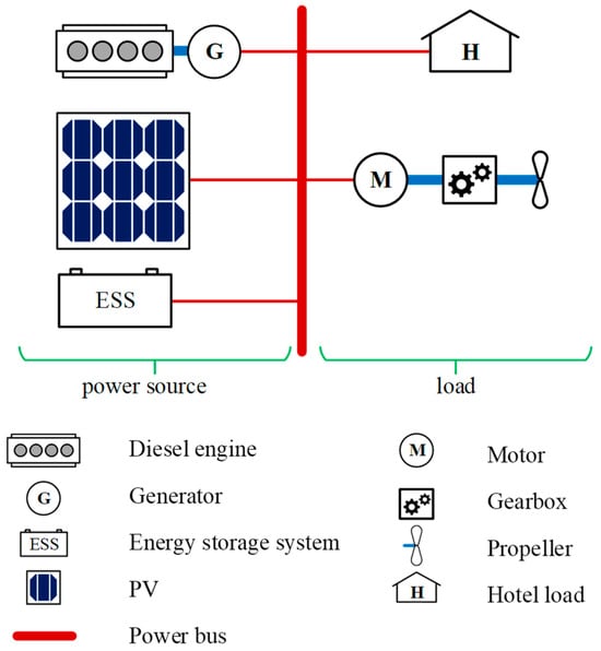
Figure 1.
Typical PV-HPS configuration.
2.1.1. Ship Dynamics
The longitudinal dynamics of the PV-HPS is given as below:
2.1.2. Hull Resistance
Besides the calm water resistance and aerodynamic resistance, which are commonly considered in existing studies [18], this study takes added resistance in waves into account.
where Rtotal, Rcw, Rair and are total resistance, calm water resistance, aerodynamic resistance and total added resistance in waves.
The calm water resistance can be calculated neglecting the wave-making resistance [29].
where k is the form factor, Cf is the frictional resistance coefficient, ρwat is the water density, Swet is the wetted area of the bare hull, Re is the Reynolds number, Lpp is the length between perpendiculars, is the kinematic viscosity of water.
The aerodynamic resistance is calculated as:
where Cair is the aerodynamic resistance coefficient, ρair is the air density, is the relative wind speed, Sair is the frontal area of the hull and superstructure.
In order to consider additional resistance in waves and investigate the effect of uncertainties related with wave, an empirical formula developed by Liu et al. is introduced [30]. The additional resistance in waves is obtained based on the added resistance in regular head waves:
where S is the wave spectrum, Raw is the added resistance in regular head waves, ζa is the wave amplitude. The JONSWAP spectrum is expressed as follows [31]:
where the peak enhancement factor γ is considered to be 3.3 [32].
The added resistance in regular head waves contains two parts that are caused by reflection/diffraction effect and motion/radiation effect, respectively [33]:
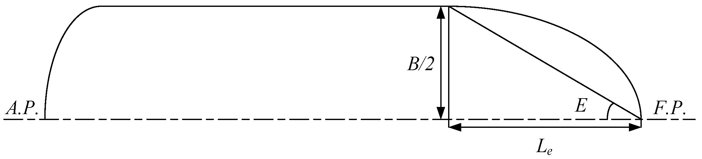
where g is the gravitational acceleration, B is the ship’s beam, αT is the draft coefficient, λ is the wave length, Fn is the Froude number, CB is the block coefficient, T is the draft of the ship. The angle of entrance of the water line E and the length of waterline entrance Le are defined in Figure 2 [33].
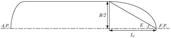
Figure 2.
Definition of length Le and angle E.
The calculation of the factors of the added resistance due to motion effect are given:
where is the resonance position of the added resistance, kyy is the longitudinal mass radius of gyration, a1, a2, a3, b1 and d1 are the factors of the added resistance due to motion/radiation effect.
2.1.3. Photovoltaic System Model
The PV system is placed horizontally on the deck, whose output mainly relies on solar radiation and PV module temperature. To strike a balance between precision and computational efficiency, the Zhou method [34] was selected to establish the PV model. On the assumption that all modules in the PV system are identical, the output power of the PV system PPVs is calculated as:
where nPV is the number of PV modules in the PV system, ηMPPT is the efficiency of the maximum power point tracking, PPVm is the maximum output power of single PV module, IPVsc, VPVoc and fPV are the short-circuit current, open-circuit voltage, and fill factor of the PV module, respectively.
The short-circuit current of PV module is given by [34]:
The open-circuit voltage is a function of solar irradiance and temperature of PV module.
The temperature of PV module is determined by the ambient temperature and solar irradiance [35].
where Ta indicates ambient temperature.
It is noted that the modeling of the rest of the system is given in Appendix A.
2.2. Energy Management Strategy
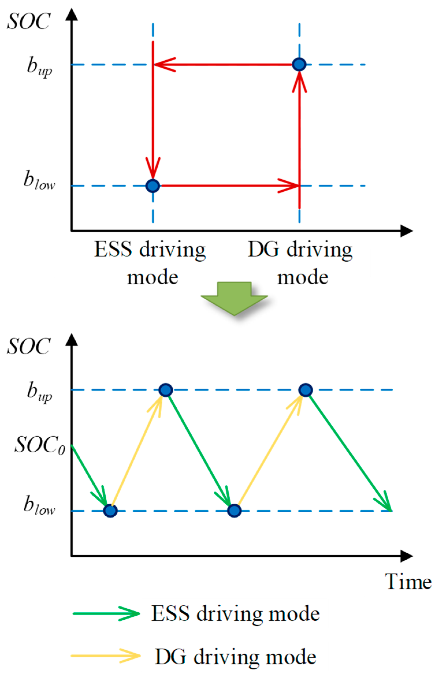
A rule-based strategy is established to control the energy distribution of the PV-HPS by virtue of its simplicity and reliability. The proposed strategy is a kind of thermostatic control strategy, which operates the PV-HPS in two modes, namely, the ESS driving mode and the DG driving mode [36]. Figure 3 explains the mechanism of such a strategy. Before the start of the voyage, the ESS is charged to SOC0. According to the mode switching strategy, the PV-HPS switches to the DG driving mode when the SOC of the ESS is smaller than the lower bound blow. In such a mode, the DG is operated at its optimal point for fuel efficiency. Here, the optimal point represents the working point with the highest efficiency (lowest specific fuel consumption (SFC)). The excess power is used to charge the ESS. If the SOC of the ESS reaches the upper bound bup, the PV-HPS switches to the ESS driving mode where the DG is shut down and the ESS supplies all power requirements.

Figure 3.
Scheme of the energy management strategy.
2.3. Uncertainty Characterization
2.3.1. Uncertainty in Power Source
According to the modeling of the PV system, the output of the PV system depends on solar irradiance and ambient temperature. Hence, the uncertainty in power source stems from the uncertainties in solar irradiance and ambient temperature, which are closely related [37]. In this study, the copula-based method is introduced to establish the JCDF of solar irradiance and ambient temperature [38].
where JFG,Ta(Gn,Ta) is the joint cumulative distribution function (JCDF) of wind speed and direction, Ct(⋅,⋅) is the t-copula function, FG(Gn) and FTa(Ta) are the cumulative distribution functions (CDFs) of normalized solar irradiance and ambient temperature, respectively; fG(Gn) and fTa(Ta) are the probability density functions (PDFs) of normalized solar irradiance and ambient temperature, respectively. Normalized solar irradiance 0 ≤ Gn ≤ 1 is calculated based on the minimum Gmin and maximum Gmax values of solar irradiance.
- (1)
- Solar irradiance
The literature suggests that the beta distribution function is the most suitable probability density function (PDF) for representing the uncertainty in solar irradiance [39]. After data normalization, the PDF of solar irradiance can be expressed as follows:
where αG and βG are the shape parameters of the beta PDF, Γ(⋅) is the gamma function, μG and σG are the mean and standard deviation obtained from the historical data.
- (2)
- Ambient temperature
Normal distribution is considered the most suitable PDF of ambient temperature [40].
where μT and σT are the mean value and standard deviation of the distribution.
2.3.2. Uncertainty in Hull Resistance
Based on the modeling of ship dynamics, the hull resistance is affected by significant wave height and wave period. Therefore, the analysis of system load cannot be achieved without characterizing the uncertainties in significant wave height and wave period. Considering the internal connection between the two parameters, a JCDF of significant wave height and wave period is required for stochastic optimization. To this end, the copula-based method is employed. For the convenience of calculation, significant wave height and wave period are normalized.
where is the JCDF of significant wave height and wave period, and are the CDFs of normalized significant wave height and wave period, respectively; and are the normalized significant wave height and wave period, respectively; and are the PDFs of significant wave height and wave period, respectively.
- (1)
- Significant wave height.
The marginal distribution of the normalized significant wave height is assumed to follow a 3-parameter Weibull distribution [41].
where αh > 0 and βh > 0 and are the scale parameter, shape parameter and position parameter of Weibull PDF.
- (2)
- Wave period
The marginal distribution of normalized wave period is assumed to be log-normally distributed in this study [41].
where ai(i = 1, 2, 3) and bi(i = 1, 2, 3) are the parameters of the log-normal distribution PDF.
2.4. Optimization Problem Formulation
2.4.1. Optimization Variables
Five design variables are considered in this study, i.e., the displacement of diesel engine in DG VD, the volume of motor rotor VM, the number of battery modules in the ESS nESS, the number of PV modules in the PV system nPV and the gear ratio of the gearbox iGB. Hence, the vector of optimization variables is expressed by:
2.4.2. Objective Function
In order to comprehensively assess the environmental and economic benefits of the PV-HPS, the greenhouse (GHG) emission and lifecycle cost are minimized in this study.
The GHG emission of the PV-HPS mainly derive from the fuel consumption of electricity generation and DG startup.
where the annual GHG emission is considered to be the product of life cycle GHG intensity of diesel fuel If and annual fuel consumption, msu is fuel consumption per startup, nsu is the number of the DG startup times.
The lifecycle cost of the PV-HEPS includes initial investment Cini, operation cost Cope and battery cost CESS.
where cDG and cM are the unit cost of the DG and motor, ΔcDG is the correction factor of electrical components in DG [42], and are the rated power of the DG and motor, cPV is the unit cost of the PV modules.
The operation cost consists of the fuel cost and the maintenance costs of the DG and PV system .
where cf is the unit cost of diesel fuel, gf is the annual inflation rate of diesel fuel, Ia is the interest rate, and are the unit maintenance cost of the DG and PV system, is the annual operation time of the DG, is the maintenance of the PV system.
where nrep is the number of battery replacements during the lifespan of the PV-HEPS Y, cESS is the unit cost of the battery module, QESS is the capacity of one battery module, gESS is the inflation rate of the acquisition cost of ESS, YESS is the lifetime of the battery module.
2.4.3. Constraints
The design parameters are optimized under the constraints of the following limits:
- (1)
- Power balance
The DG, PV system, and ESS collectively provide the electricity load that includes motor power requirements and hotel load.
- (2)
- Constraints of the DG
The DG is required to have the ability to provide for navigational safety.
where is the maximum output of the DG.
A specific duration must be exceeded between two consecutive startup/shutdown operations [43].
where ton/off(k) is the time that a startup/shut-down operation happens.
- (3)
- Constraints of the ESS
The SOC and current of the battery are constrained for safety.
where and represents the current limit for charging and discharging.
2.5. Optimization Methodology
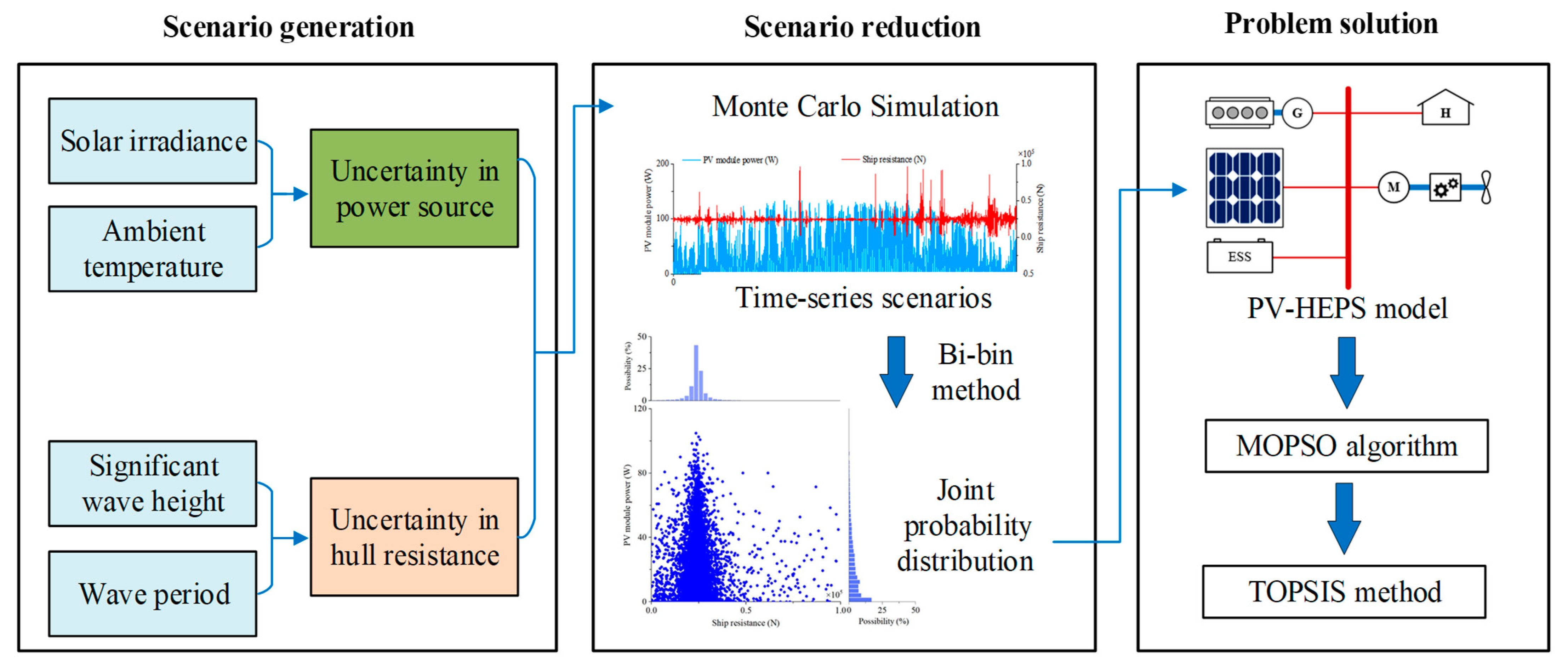
Monte Carlo (MC) simulation is a popular tool addressing the uncertainties in power system optimization, and is used in this study to handle the uncertainties in solar irradiance, ambient temperature, significant wave height and wave period. In general, about 1000 scenarios are considered to be sufficient to guarantee the convergence of MC [44]. However, such number of simulation trials leads to huge computational burden. Therefore, a bi-bin method is introduced in the optimization methodology for scenario reduction, due to its efficiency in handling large datasets [45]. By discretizing time-series scenarios into bins, the bi-bin method significantly reduces computational burden. It converts a large number of time-series scenarios of environmental conditions into a smaller set of discrete scenarios of PV module power and hull resistance with corresponding probabilities, thereby alleviating the computational load. Figure 4 depicts the framework of the proposed optimization methodology. Three key steps are listed as follows:
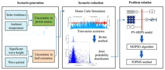
Figure 4.
Framework of the optimization methodology.
- Step 1: scenario generation.
The Monte Carlo (MC) simulation is performed to generate nMC = 1000 time-series scenarios for solar irradiance, ambient temperature, significant wave height and wave period considering their coordinated variation based on the two joint distributions given before. Then, time-series scenarios for PV module power and hull resistance are obtained with the help of the PV-HPS model. It’s worth noting that PV module power and hull resistance are cross-correlated and should be matched at each time point.
The scenario generation process is performed as follows. (1) JCDF Sampling: draw random samples from the JCDF, representing the joint distributions of key environmental variables. (2) CDF calculation: use copula functions to calculate the cumulative distribution functions (CDFs) of solar irradiance, ambient temperature, significant wave height, and wave period. (3) Variables calculation: convert these CDF values into numerical values of the environmental variables based on their marginal distribution models.
- Step 2: scenario reduction.
(1) Discretization: Time-series scenarios for PV module power and hull resistance are discretized into one-hour intervals. A joint probability distribution of PV module power and hull resistance is then established;
(2) Interval Division: Divide the ranges of PV module power and hull resistance into kbin equal intervals, respectively;
(3) Bin Creation: Create a two-dimensional space of bins by combining the intervals of PV module power and hull resistance;
(4) Scenario Allocation: Place each discrete scenario (pair of PV module power and hull resistance) into the corresponding bin based on its values;
(5) Scenario Averaging: For each bin, compute the average values of PV module power and hull resistance for the scenarios within the bin. These averages represent the characteristic scenario for that bin. Count the number of scenarios in each bin and calculate the probability of each characteristic scenario by dividing the count by the total number of scenarios.
Up to this point, nMC time-series scenarios for solar irradiance, ambient temperature, significant wave height and wave period are transformed into pairs of module power and hull resistance that will be used as scenarios in the following process. In this way, the data length is not related to the number of MC simulations nMC, but to the number of bins.
In order to guarantee the fairness of comparison, when each one-hour scenarios terminate, the SOC of the ESS is adjusted back to its initial value, SOC0, using fuel consumption compensation method. That is, based on the efficiency of the diesel generator set at the optimal (highest efficiency) point, the change of the battery SOC is converted into fuel consumption.
- Step 3: Problem solution.
The joint probability distribution of PV module power and hull resistance is sent to the PV-HPS model, which is then employed by the classical multi-objective particle swarm optimization (MOPSO) algorithm [46] to solve the optimization problem. The velocity update is performed based on the following equations.
where is the speed vector of particle i at kth iteration, is the position of particle i at kth iteration, is the inertia, r1 and r2 are two random numbers with uniform distribution from [0 1], c1 is the particle increment, c2 is the global increment, is the best position experienced by particle i, is the global best position experienced by all particles.
To prevent velocities from becoming excessively large and causing particles to exceed the search space boundaries, velocity limitations are implemented [47]. This is particularly important when particles are far from their personal and global best positions.
where is jth dimension of speed vector , is the velocity limit factor, xj,max and xj,min are the upper and lower bound of jth dimension of .
Note that the duration of the scenarios generated by the joint probability distribution is set to be 1 h. Here, to carry out an overall evaluation for PV-HPS performance, the objective function is modified.
where f1ij(x) and f2ij(x) are the GHG emission and lifecycle cost of PV-HPS under scenario Sij(i = 1, 2, …, k, j = 1, 2, …, k), pij is the probability of bin Bij(i = 1, 2, …, k, j = 1, 2, …, k). Here, only non-empty bins are considered in this step to speed up the optimization. The Technique for Order Preference by Similarity to an Ideal Solution (TOPSIS) method is subsequently employed to rank the Pareto designs and facilitate the selection of the final design [48].
3. Results and Discussion
3.1. Case Study
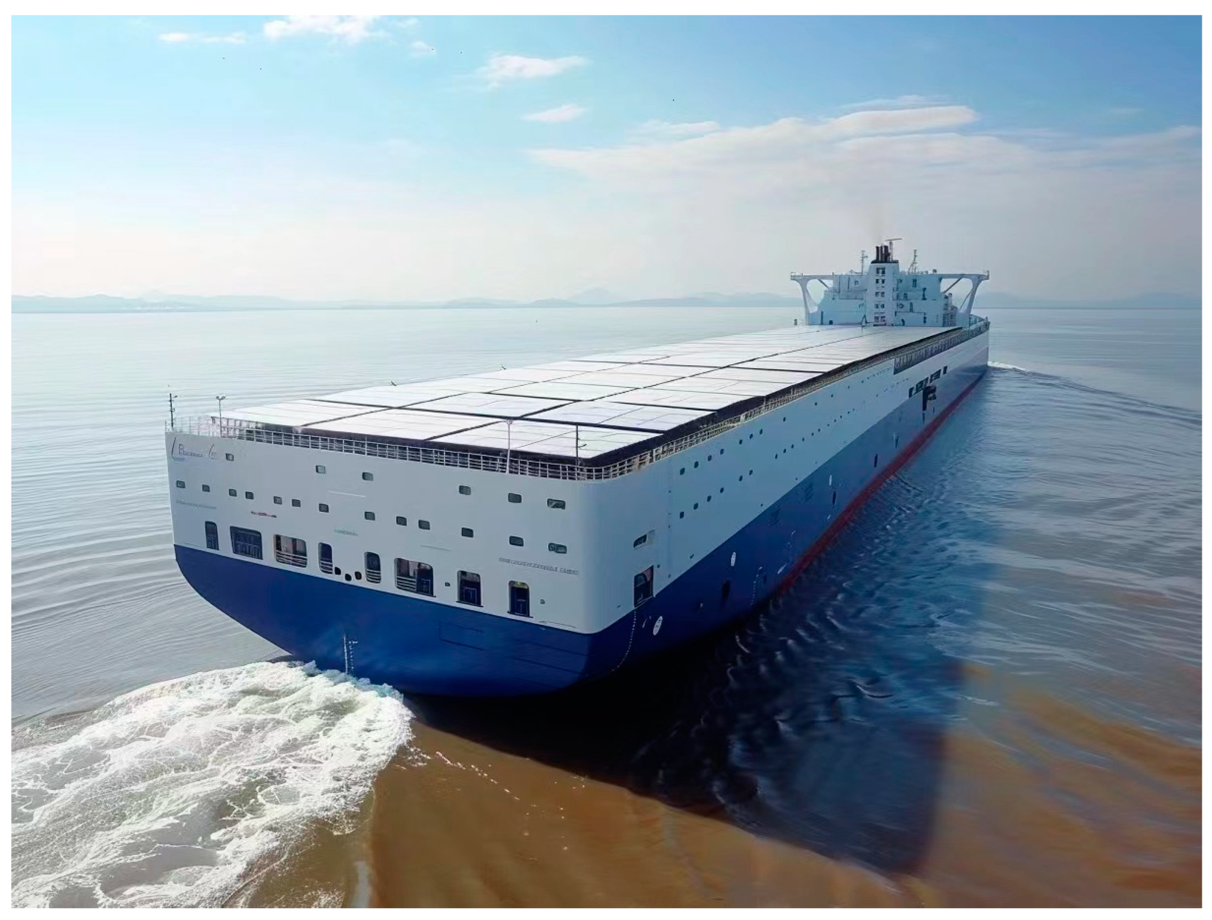
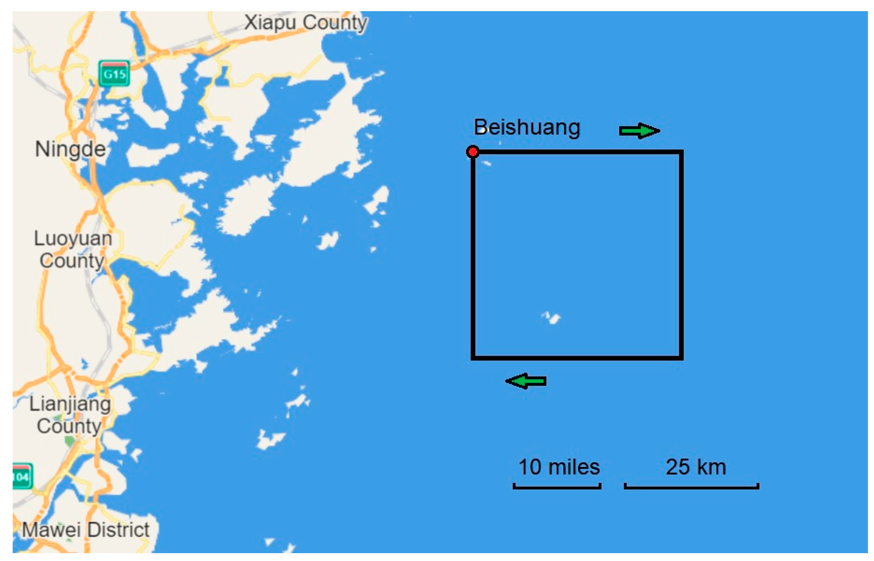
With the advancement of China’s Marine Power Strategy, the demand for monitoring meteorological and hydrological environments and detecting fishery resources has significantly increased. Unmanned ships have the advantages of low cost and high safety, and can independently carry out data collection and transmission work without relying on drivers. Therefore, the development of green unmanned ships is of great importance for hydrological monitoring, fishery management and combating smuggling. Therefore, the proposed methodology is tested by the design of a PV-HPS for an unmanned ship which usually operates in the Beishuang area (26.7° N 120.3° E) of the East China Sea. As is shown in Figure 5, the PV system is placed horizontally on the deck of the case ship. The main dimensions of the ship are presented in Table 1. Figure 6 illustrates the route of a square with sides spanning 24 nautical miles (about 44.45 km). Every day, the ship leaves the port at 7:00 a.m. and navigates at a speed of 8 kn (4.11 m/s). After returning to the port at 18:00 p.m., the ship is refueled and the ESS is charged to the SOC of SOC0. The hotel load is assumed to be 10 kW. PV modules are installed on the deck and the top of the superstructure to take the most advantage of solar energy. The following assumptions have been made: (1) the unmanned ship is strictly sailing according to the prescribed route and speed, (2) the situation of being unable to sail due to extreme sea conditions or other low-probability events is ignored, (3) the impact of the energy system sizing on the dynamic parameters of the ship is ignored.

Figure 5.
Case study ship.

Table 1.
Main dimensions of the case study ship.

Figure 6.
Navigation route.
Data of solar irradiance, ambient temperature, significant wave height and wave period in the Beishuang area from 2011 to 2020 were obtained from the China Meteorological Data Service Center and used for uncertainty characterization. Figure 6 presents the hourly data of the four environmental parameters in 2020. Note that only the data during sailing time (7:00 to 18:00) is shown. In Figure 6, significant fluctuations can be found, which shows uncertainties in solar irradiance, ambient temperature, significant wave height and wave period. As aforementioned, the neglect of such uncertainties inevitably leads to misevaluation of the performance of PV-HPS, resulting in sub-optimal designs. To highlight the necessity of considering environmental uncertainties and the effectiveness of the proposed method, a deterministic optimization is performed with the environmental parameters in 2020. In addition, two partial stochastic optimizations that consider two of the four uncertain parameters are also proposed as controls. The uncertainties considered in the optimizations are listed in Table 2. The ranges of optimization variables are given in Table 3. The parameters required in the optimization are given in Table A1. All the work is performed on a computer with a 12th Gen Intel(R) Core (TM) i5-12500H CPU of 3.10 GHz and a memory size of 16.00 GB. The parameters of the MOPSO algorithm are given in Table A2.
Table 2.
Uncertainties considered in the optimizations.
Table 3.
Results of stochastic optimization and deterministic optimization.
3.2. Statistical Characteristic of Stochastic Scenarios VD (10−3m3)
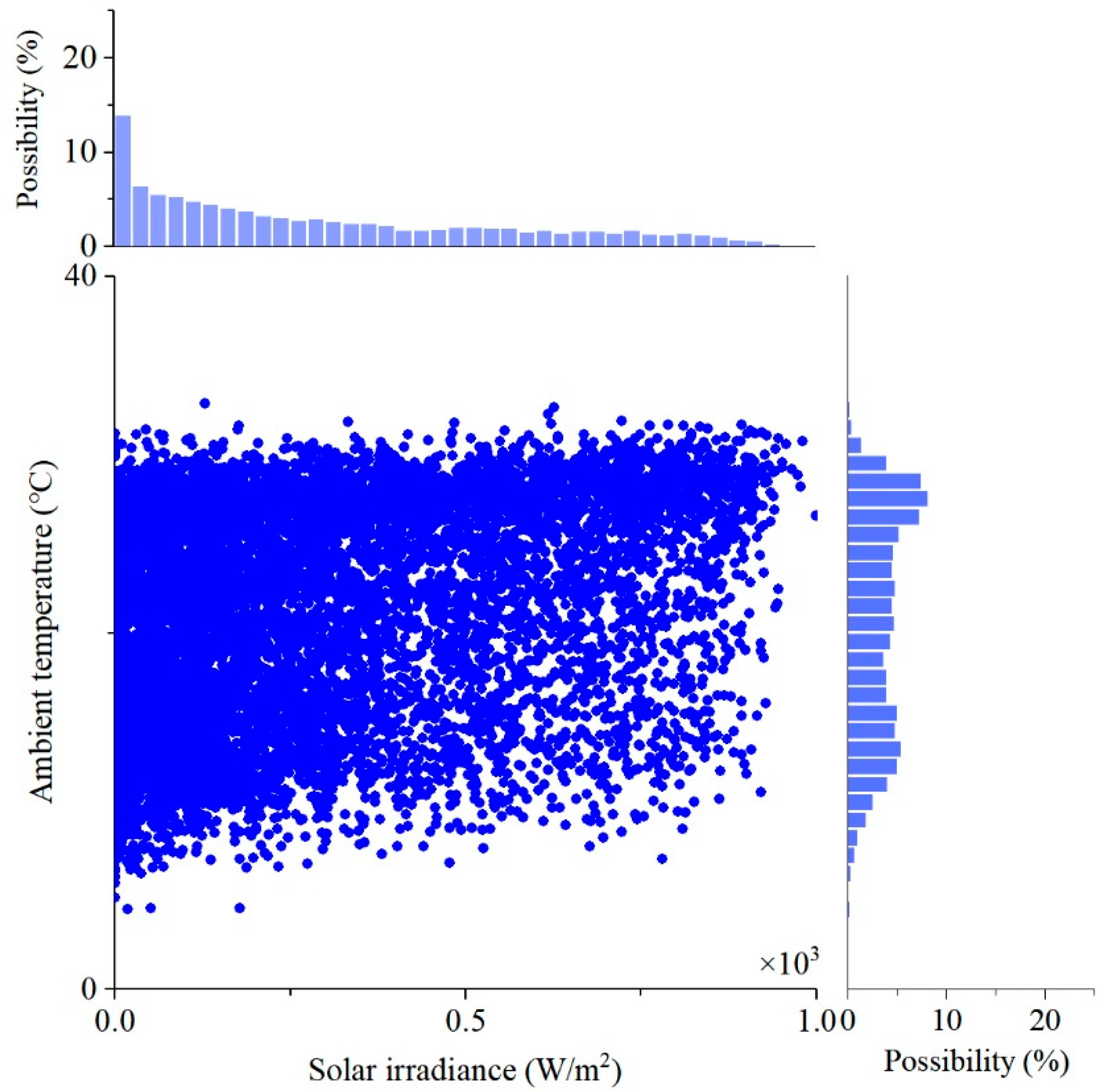
The joint probability distribution, as presented in Figure 7, is employed to investigate the relationship between solar irradiance and ambient temperature. The Pearson correlation coefficient of the two parameters is 0.34, indicating that there is a positive but weak correlation between solar irradiance and ambient temperature. Figure 8 illustrates the joint probability distribution of significant wave height and wave period. The Pearson correlation coefficient is 0.27, indicating a weak positive correlation between the two environmental variables. No distinct linear correlation can be recognized in Figure 7 and Figure 8. Hence, it becomes necessary to employ the copula-based method for uncertainty characterization, as it possesses the ability to effectively describe the nonlinear correlations between uncertainties.
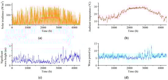
Figure 7.
Solar irradiance, ambient temperature, significant wave height and wave period of the Beishuang area in 2020: the data was collected from 07:00 to 18:00 each day. (a) solar irradiance; (b) ambient temperature; (c) significant wave height; (d) wave period.

Figure 8.
Joint probability distribution of solar irradiance and ambient temperature.
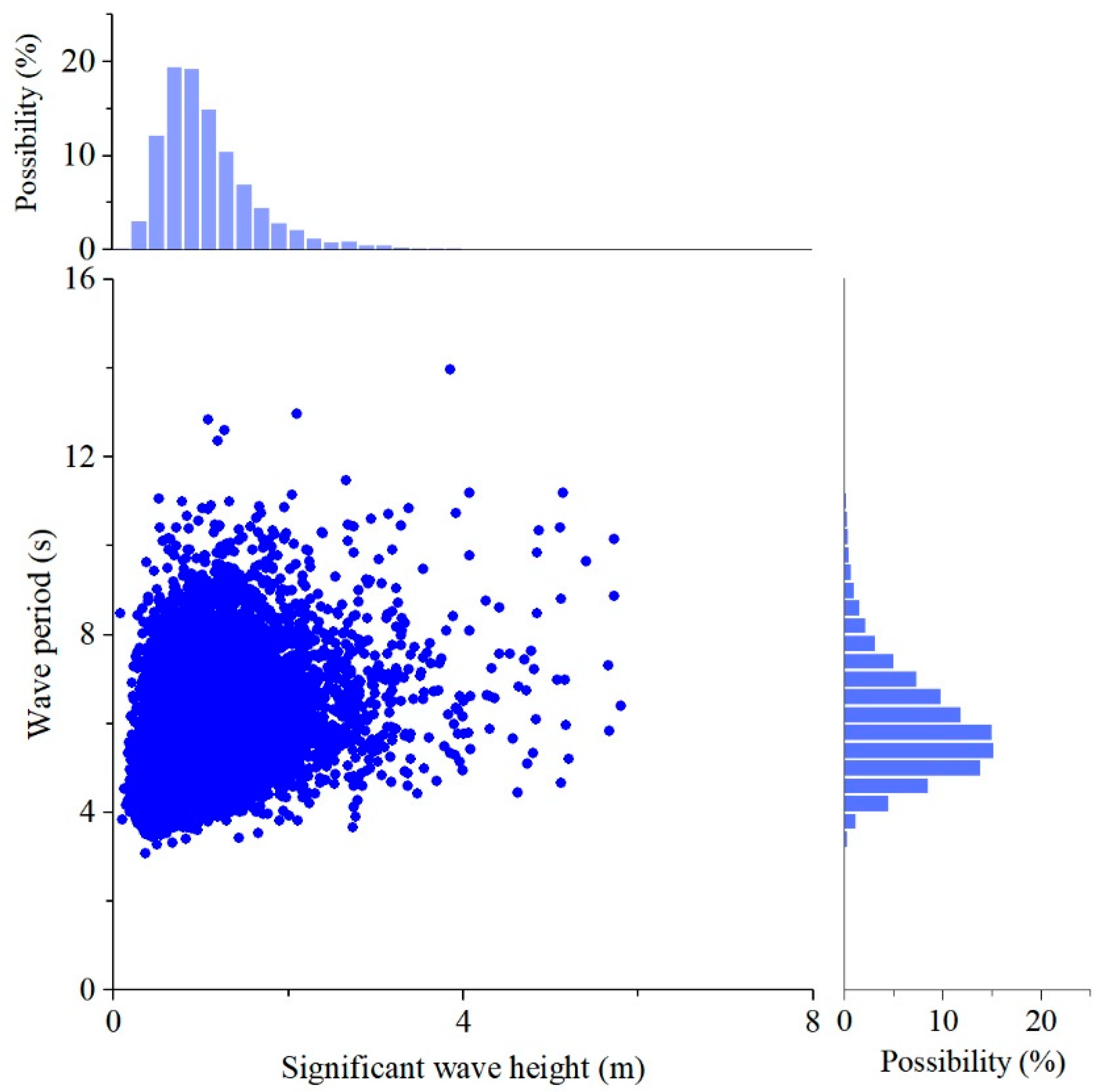
The joint probability distribution of PV module power and hull resistance is shown in Figure 9. It is found that the ship resistance approximately follows a to normal distribution with the expectation of 2.5 × 10⁴ (N). On the other hand, the distribution of PV module power is more closely aligned with an exponential distribution. The PV module power is less than 20 W in over 50% of cases. Two factors are responsible for this. First, the solar irradiance of the Beishuang area is not high enough, especially in spring and winter. Second, only a small amount of solar energy can be used by the PV module in the early morning and at dusk. The Pearson correlation coefficient of PV module power and hull resistance is 0.00. Therefore, the effect of uncertainties on the PV-HPS should be investigated in terms of PV module power and hull resistance, respectively.
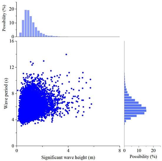
Figure 9.
Joint probability distribution of significant wave height and wave period.
3.3. Optimization Results
A probabilistic simulation is conducted over the Pareto front (PF) solutions obtained by the four optimizations (Table 3) to evaluate the average performance of the solutions in real life and assess the effect of uncertainties on optimization. The four groups of PF solutions are simulated with 1000 time-series stochastic scenarios generated in Step 1 of the proposed optimization method. Those scenarios are assumed to be competent to represent various working conditions of the PV-HPS in its lifespan.
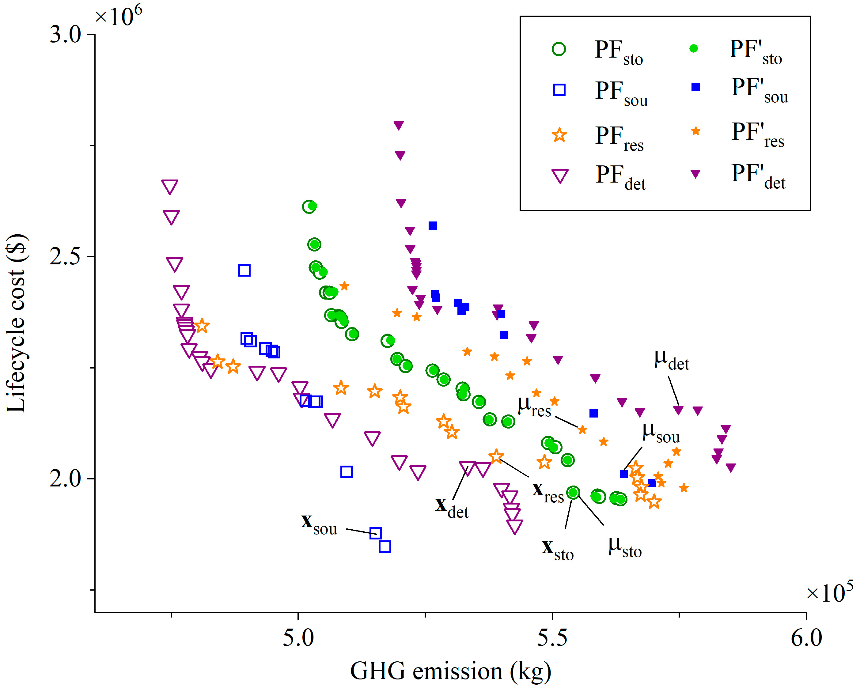
The mean performance of the four optimizations is shown in Figure 10 with solid icons. It is observed that the PF of stochastic optimization, PFsto, is located at the upper right of the PF of deterministic optimization, PFdet, as do the PFs of the two partial stochastic optimizations. However, the PFs of the deterministic optimization and two partial stochastic optimizations move to the upper right of PFsto when the uncertainties in solar irradiance, ambient temperature, significant wave height and wave period are introduced. For example, the final solution of the deterministic optimization xdet produces 5.33 × 10⁵ kg of GHG emissions annually and requires $2.02 × 10⁶ of lifecycle cost. After the probabilistic simulation, the mean value of the objectives (represented by μdet in Figure 10) moves to 5.74 × 10⁵ kg of GHG emissions (increases by 7.69%) and $2.16 × 10⁶ of lifecycle cost (increases by 6.93%), respectively. This indicates that the ignorance of all or parts of uncertainties leads to overvaluation of PV-HPS performance.
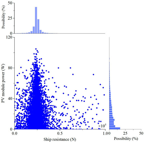
Figure 10.
Joint probability distribution of PV module power and ship resistance.
In addition, the PF of partial stochastic optimization of hull resistance, PFres, which takes the uncertainties in significant wave height and wave period into consideration, is closer to the PF of stochastic optimization than its counterparts. Analogously, the average Euclidean distance moved by the solutions in PFres after the probabilistic simulation is also the lowest among the three controls. This demonstrates that the uncertainties in significant wave height and wave period, which relate to hull resistance, are the major factors affecting the optimization results. It is worth noting that the PF of the stochastic optimization almost coincides with its mean performance after the probabilistic simulation. Hence, the capability of the proposed stochastic optimization method in uncertainty characterization can be verified.
Table 3 lists the final solutions of the four optimizations found by the TOPSIS method. The optimal solution given by the proposed stochastic optimization method, xsto, achieves 5.54 × 10⁵ kg of GHG emissions and $1.97 × 10⁶ of lifecycle cost that are 3.48% and 8.84% lower, respectively, compared with the mean performance μdet of the deterministic solution, xdet, when uncertainties are considered. According to Table 3, small DGs, motors, and ESSs are used in the four solutions because of the low initial investment. However, the constraint of maximum power of the DG prevents VD, VM, and nESS from further decreasing. It is observed that the deterministic optimization and the partial stochastic optimization considering hull resistance related uncertainties result in a higher number of PV modules compared with the other two optimizations that take uncertainties in solar irradiance and ambient temperature into consideration. The reason behind this is the overestimate of PV module power by ignoring the uncertainties in solar irradiance and ambient temperature. Consequently, more than necessary PV modules are installed to make the most of solar energy.
It is noteworthy that the proposed method in this paper can be applied to other similar problems. For instance, by adjusting the model parameters, various types of ship models can be constructed. With the proposed method, environmental data of different sea areas can be used to generate stochastic scenarios of different routes. Thus, power systems can be designed for ships with different navigation areas and tasks.
3.4. Sensitivity Analysis of Bin Number
The optimal sizing of the PV-HPS performed in the previous sections shows that the stochastic optimization method proposed in this study can deal with the cross-correlated uncertainties of solar irradiance, ambient temperature, significant wave height, and wave period. However, in the mathematical sense, different bin numbers () would express different features of the power source (PV module power) and system load (hull resistance), leading to different optimization solutions accordingly. It is easy to imagine that a larger bin number is likely to offer a greater ability in uncertainty characterization at the expense of higher computational complexity. On the contrary, a smaller bin number reduces the computing effort but may end up with a solution with dissatisfactory performance in real life. Hence, a sensitivity analysis is proposed in this section to investigate and determine the appropriate bin number. In the sensitivity analysis, the stochastic optimization is conducted with different kbin, namely, different bin numbers (). Then, the probabilistic simulation is also proposed where the final solutions are simulated with 1000 time-series uncertainty scenarios generated in Step 1 to evaluate their mean performance in real life. The settings used in the sensitivity analysis are listed in Table 4.
Table 4.
Settings and results of the sensitivity analysis.
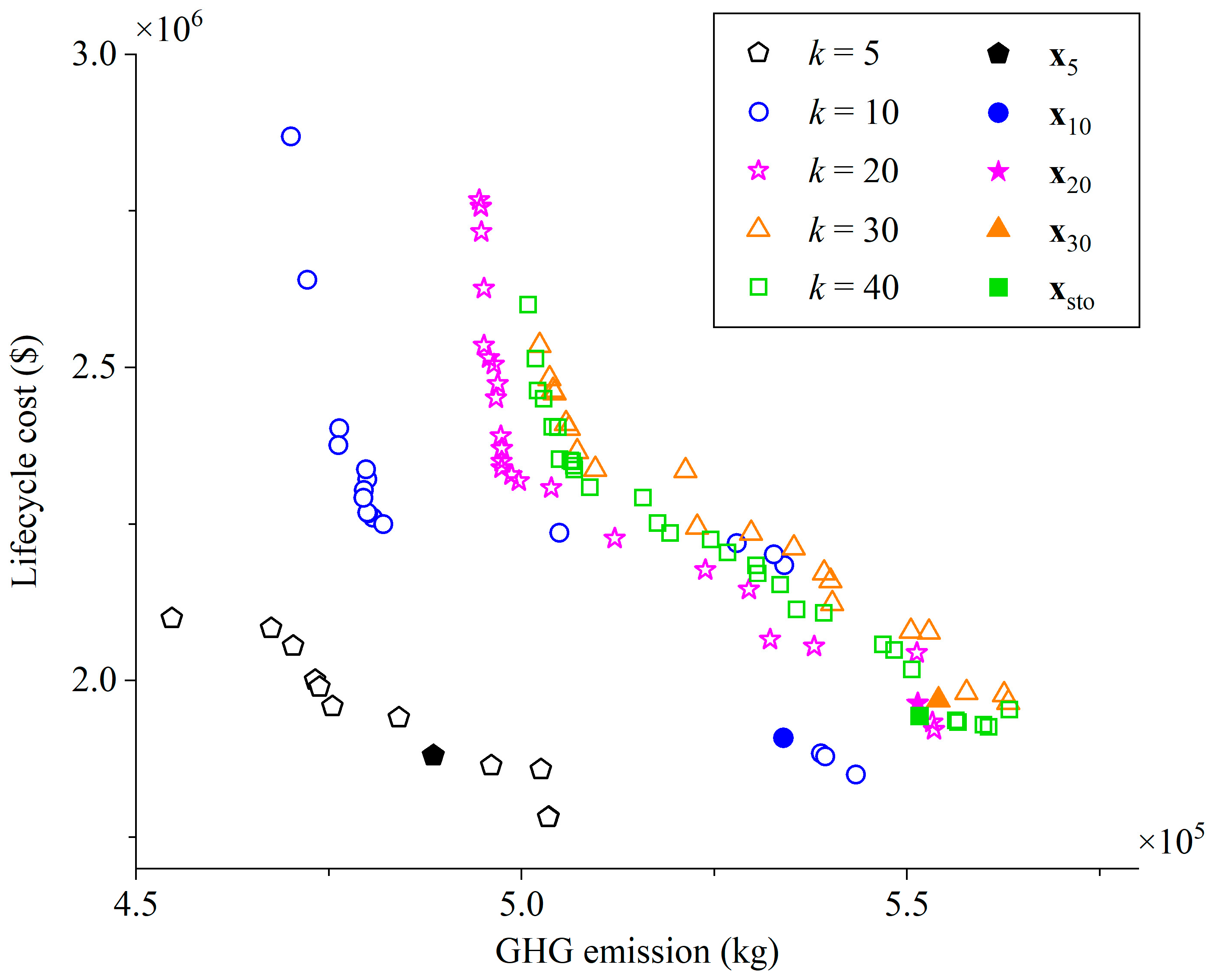
Figure 11 shows the PFs of the optimizations obtained in the sensitivity analysis. The final solutions of the optimizations found by the TOPSIS method are labeled with solid icons. When kbin = 5, PF5 is located in the lower left of Figure 11. The PFs move to the upper right as kbin increases. In addition, the distance between two consecutive PFs decreases at the same time. The PF of kbin = 30, PF30, almost coincides with that of kbin = 40 (PF40). Figure 12 compares the final solutions obtained with different kbin. It is observed that all stochastic optimizations result in solutions outperforming the solutions provided by the deterministic optimization. This highlights the importance of considering the uncertainties in solar irradiance, ambient temperature, significant wave height, and wave period. It is also found that the GHG emissions and lifecycle cost increase with kbin, whereas the mean performance of the solutions decreases with kbin when the uncertainty scenarios are introduced.
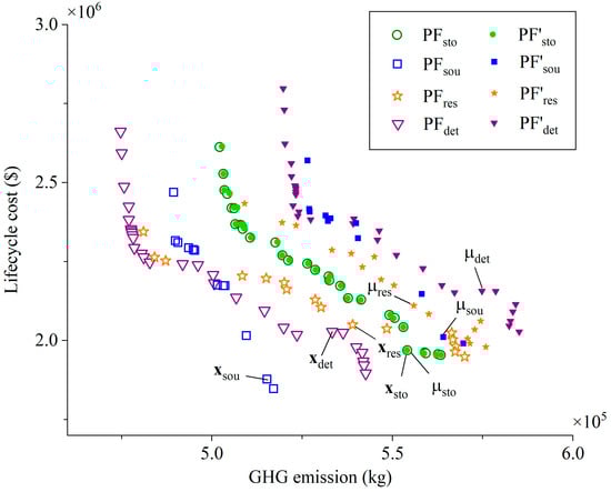
Figure 11.
Pareto front of stochastic optimization and deterministic optimization. PFsto: Pareto front (PF) of stochastic optimization, PFsou: PF of the partial stochastic optimization considering uncertain power source, PFres: PF of the partial stochastic optimization considering uncertain hull resistance, PFdet: Pareto front of deterministic optimization. PF’sto, PF’sou, PF’res and PF’det are the mean performance of solutions in PFsto, PFsou, PFres and PFdet under stochastic scenarios. μsto, μsou, μres and μdet represent the mean performance of solutions of xsto, xsou, xres and xdet under stochastic scenarios, respectively.
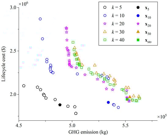
Figure 12.
Pareto fronts obtained with different kbin.
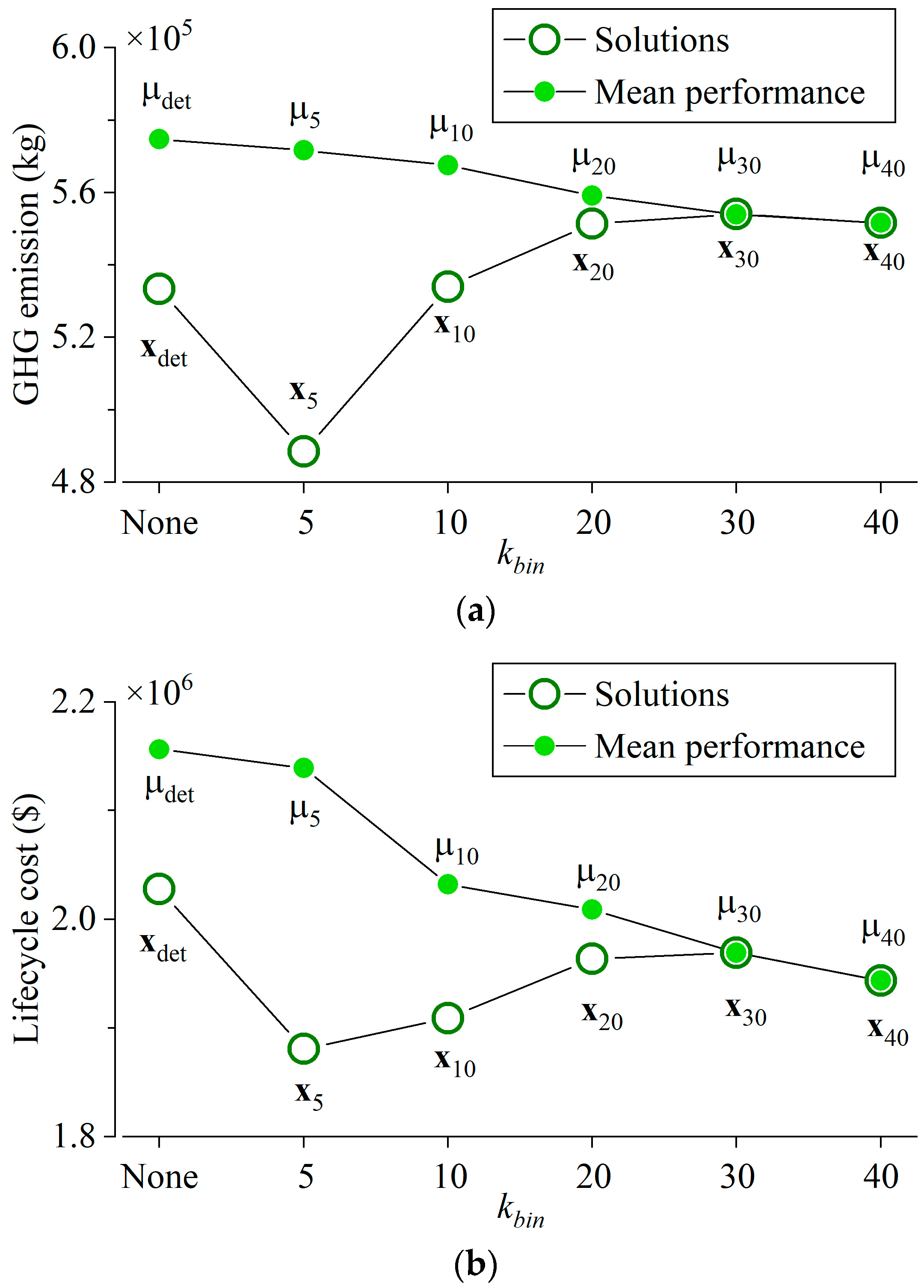
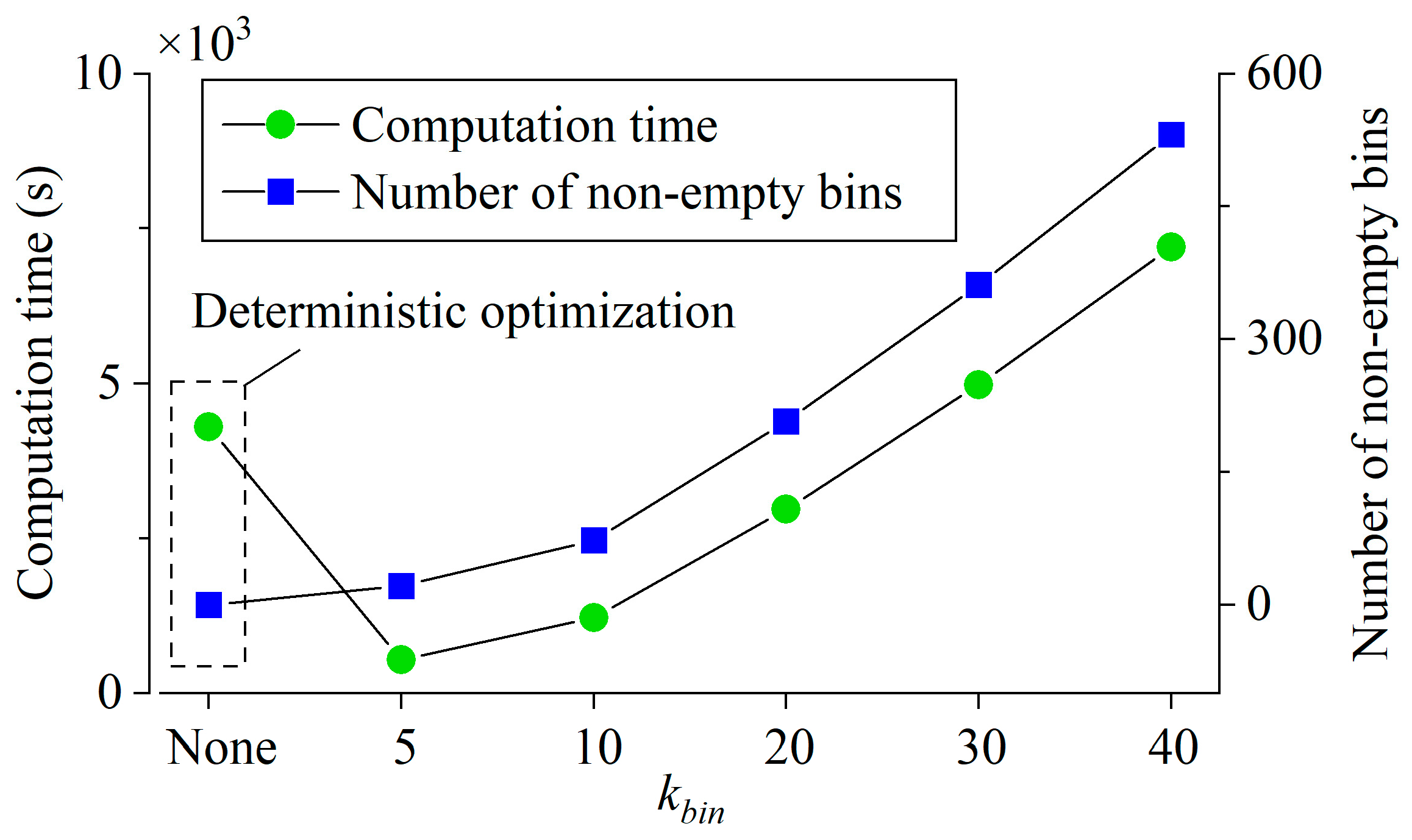
As can be seen in Table 4, the difference between the final solutions and their mean performance under uncertainty scenarios converges to a small neighborhood of zero as long as kbin reaches 30, i.e., the lengths of the bin sides are 5.5 kW and 5000 N, respectively. As depicted in Figure 13 and Figure 14, the computational time increases along with the number of non-empty bins as kbin increases. It takes 3000 s to finish the stochastic optimization with kbin = 20. When k increases to 40, 7250 s is required by the optimization process. Those results prove that more bins contribute to uncertainty characterization within limits, resulting in better solutions, but leading to a higher computational burden. Taken together, kbin = 30 (bin number = 900) gains a satisfactory tradeoff between solution optimality and computational complexity. Compared with the solution of the deterministic optimization xdet, the solution x30 achieves 3.37% GHG emission and 8.88% cost savings at the expense of 690 s more computation time, which is acceptable in the design stage of the PV-HPS.

Figure 13.
The final solutions obtained with different kbin. (a) GHG emission; (b) lifecycle cost.
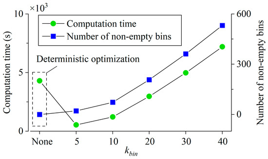
Figure 14.
Computational complexity with different kbin.
The findings of this study, while focused on an unmanned ship, have broader applicability to other types of vessels. The stochastic optimization method proposed for PV-HPS can be adapted to different vessel types by adjusting the input parameters and constraints specific to each vessel’s operational profile and design characteristics. The methodology’s flexibility in handling various environmental uncertainties and its capability to minimize GHG emissions and lifecycle costs make it suitable for a wide range of maritime applications, including commercial ships, passenger vessels, and naval ships.
4. Conclusions
In this study, a stochastic optimization approach, based on MC simulation, bi-bin scenario reduction technique, and MOPSO algorithm, is proposed for the sizing of the PV-HPS, aiming to minimize GHG emissions and lifecycle cost. To examine the stochastic behavior and synergistic effect of uncertainties in solar irradiance, ambient temperature, significant wave height, and wave period, joint distributions of environmental uncertainty sources associated with PV module power and hull resistance are established. The case study indicates that the proposed stochastic model outperforms deterministic optimization and two partial stochastic optimizations.
Moreover, the trade-off between solution optimality and computational complexity is investigated in the sensitivity analysis of bin numbers. It is observed that a large bin number is beneficial to uncertainty characterization and performance enhancement of the PV-HPS, albeit at the cost of higher computational burden. A satisfactory balance between system performance and computational complexity is achieved with kbin = 30.
In terms of future work, the uncertainties related to other energy conversion equipment, such as the aging of DGs and batteries, as well as uncertainties in component and fuel prices should be considered to improve the performance evaluation of the PV-HPS over its lifespan. The seasonal characteristics of uncertainties should also be investigated, especially for studies focused on optimal operation. Furthermore, in order to further enhance the environmental and economic benefits of ships, different types of renewable energy resources, such as sails and fuel cells, should be incorporated into the system in addition to the PV module.
Author Contributions
J.Z.: Conceptualization, Investigation, Methodology, Software, Visualization, Writing—original draft. L.C.: Conceptualization, Funding acquisition, Resources, Supervision, Writing—review and editing. All authors have read and agreed to the published version of the manuscript.
Funding
This research was funded by the National Key R&D Program of China, 2022YFB4300803, and the Oceanic Interdisciplinary Program of Shanghai Jiao Tong University, WH410260401/006.
Institutional Review Board Statement
Not applicable.
Informed Consent Statement
Not applicable.
Data Availability Statement
The data that support the findings of this study are available from the corresponding author, Li Chen, upon reasonable request.
Conflicts of Interest
The authors declare no conflict of interest.
Appendix A
Appendix A.1. Propeller Model
The thrust Tpro and torque Qpro of the propeller are given by [49]:
where KT is the thrust coefficient, Dpro is the propeller diameter, KQ is the torque coefficient, npro is the propeller speed in revolution per minute. The values of KT and KQ can be found in the Wageningen B-screw series [50].
Appendix A.2. Gearbox Model
The propeller is driven by the motor through a gearbox. Considering the mechanical loss, the output power of the motor is written as:
where is the motor speed, TM is the motor torque, iGB and ηGB are the gear ratio and efficiency of the gearbox, respectively.
Appendix A.3. Motor Model
To achieve component sizing, a scalable model of the motor is established with the Willans line method [51]. The efficiency ηM of the motor equals the ratio of output power to input power .
The input power of the motor can be calculated using three intermediate variables, namely, MEP, AMEP, and MEP loss of the motor [52].
where VM, dM and lM are the volume, diameter and length of the motor rotor, respectively. The shape factor iM equals to the ratio between dM and lM. According to Rizzoni’s study [53], the parameterizations of Equation (A8) can be:
where is the velocity of a point at the rotor surface. The Willans factors eMij(i = 0, 1, l; j = 0, 1, 2) are identical for motors in the same category [53] and can be calculated by least-squares fitting based on the efficiency map of baseline motor.
Substituting (A10) and (A11) into (A13), velocity of a point at rotor surface is obtained.
Assuming iM is a constant, the relationship between the input and output of a newly designed motor can be obtained according to Equation (A12) by changing VM.
Appendix A.4. Diesel Engine Model
Analogous to the motor, the Willans line method is also used to describe the efficiency of the diesel engine based on the intermediate variables, i.e., MEP and AMEP of the diesel engine.
where HLHV is the lower heating value of fuel, is the mass flow of diesel fuel, and TD are the speed and torque of the diesel engine, respectively. The engine cylinder displacement VD is a function of stroke SD and bore BD.
Assuming that the bore/stroke ratio iD is constant, the stroke and bore of the diesel engine can be represented by the engine cylinder displacement and iD.
The average piston speed vD is:
The relationship between pDe and pDa is then defined by [53]:
where the Willans factors eDij(i = 0, 1, l; j = 0, 1, 2) are considered to be constants for diesel engines belong to the same category [53]. Changing the value of displacement, the mass flow of a scaled engine can be calculated by substituting (A15) and (A16) into (A22).
Appendix A.5. Generator Model
The generator is fed by the diesel engine and provides power to the PV-HPS system. To ensure the efficiency and reliability of the DG, the generator is chosen to match the diesel engine.
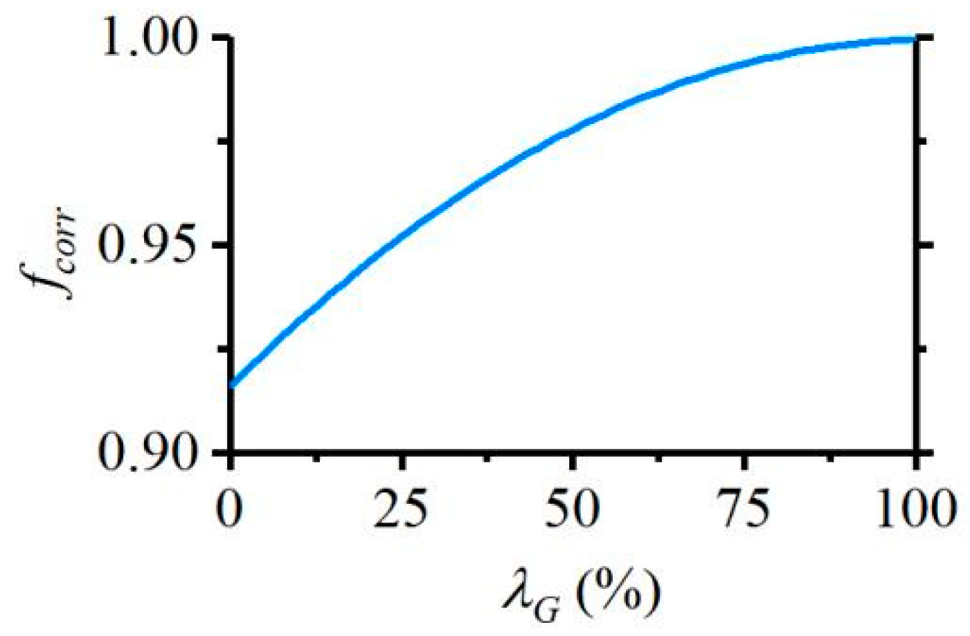
where SG is the binary factor that describes the on/off state of the generator, ηG is the efficiency of the generator.
where ηG0 is the efficiency of the generator at its rated power, is the rated power of the generator. The deviation factor of generator efficiency fcorr(λ) is a function of normalized power λG of the generator. The value of fcorr(λ) can be found in Figure 14 [54].

Figure A1.
Deviation factor of generator efficiency.
Figure A1.
Deviation factor of generator efficiency.
Appendix A.6. Energy Storage System Model
The energy storage system (ESS) is constituted by battery modules, which consist of 40 lithium-ion battery cells. On the assumption that the dynamics of all batteries are identical, batteries share the same state of charge (SOC) as the ESS system.
where nESS is the number of battery modules in the ESS, SOCbat and SOCESS are the state of charge of one battery and the ESS, respectively. PESS is the output power of the ESS.
The battery is modeled with an equivalent circuit model for simplicity [55].
where ηcolm is Coulombic efficiency, Vbat, Rbat and Qbat are the open circuit voltage, internal resistance and capacity of the battery, respectively.
Appendix B
Table A1.
Parameters used in the optimization.
Table A1.
Parameters used in the optimization.
| Parameter | Value |
|---|---|
| Cair | 0.80 |
| Cs ($) | 5000.00 |
| cDG ($/kW) | 350.00 [42] |
| ($/h) | 0.02 [56] |
| cf ($/t) | 520.00 [57] |
| cM ($/kW) | 32.00 [42] |
| CPV ($/kW) | 6500.00 [58] |
| ($/kW) | 35.00 [58] |
| G0 (w/m2) | 1000.00 [34] |
| gESS (%) | 3.00 [59] |
| gf (%) | 3.00 [59] |
| HLHV (J/kg) | 4.27 × 10⁷ [60] |
| Ia (%) | 5.00 [59] |
| (A) | 82 |
| (A) | −41.00 |
| IF | 3.71 [61] |
| IPVsc0 (A) | 6.50 [58] |
| iD | 0.82 |
| iM | 1.92 |
| K (J/K) | 1.38 × 10⁻²³ |
| m (kg) | 1.14 × 10⁶ |
| nMC | 1000 |
| PSh (W) | 5000.00 |
| (W) | 200,000 |
| Qbat (Ah) | 41.00 [42] |
| q (C) | 1.6 × 10⁻¹⁹ |
| Sair (m2) | 60.50 |
| Swet (m2) | 680.00 |
| SOC0 (%) | 50.00 |
| 40.00 | |
| 60.00 | |
| T (m) | 3.15 |
| TPV0 (K) | 298.15 |
| (s) | 60.00 |
| (h) | 2.99 × 10⁴ |
| tP | 0.10 [62] |
| VPVoc0 (V) | 21.00 [58] |
| Y (year) | 25.00 |
| YESS (year) | 5.00 [12] |
| γPV | 1.15 [34] |
| ΔcDG (%) | 6.00 [57] |
| ρair (kg/m3) | 1.29 |
| ρw | 1.03 × 10³ [62] |
| ηG0 | 0.97 [54] |
| ηGB | 0.98 [63] |
| ηMPPT | 95% [64] |
Table A2.
Parameters of MOPSO algorithm.
Table A2.
Parameters of MOPSO algorithm.
| Parameters | Value |
|---|---|
| Maximum iterations | 50 |
| Number of particles | 40 |
| Inertia | 0.4 |
| Global increment | 0.9 |
| Particle increment | 0.9 |
| Velocity limit factor | 0.1 |
References
- Faber, J.; Hanayama, S.; Zhang, S.; Pereda, P.; Comer, B.; Hauerhof, E.; van der Loeff, W.S.; Smith, T.; Zhang, Y.; Kosaka, H.; et al. Fourth IMO GHG Study 2020 Executive Summary; IMO: London, UK, 2021; pp. 1–524. [Google Scholar]
- Vahabzad, N.; Mohammadi-Ivatloo, B.; Anvari-Moghaddam, A. Optimal energy scheduling of a solar-based hybrid ship considering cold-ironing facilities. IET Renew. Power Gener. 2021, 15, 532–547. [Google Scholar] [CrossRef]
- Park, C.; Jeong, B.; Zhou, P. Lifecycle energy solution of the electric propulsion ship with Live-Life cycle assessment for clean maritime economy. Appl. Energy 2022, 328, 120174. [Google Scholar] [CrossRef]
- Yuan, Y.; Wang, J.; Yan, X.; Shen, B.; Long, T. A review of multi-energy hybrid power system for ships. Renew. Sustain. Energy Rev. 2020, 132, 110081. [Google Scholar] [CrossRef]
- Fan, A.; Li, Y.; Liu, H.; Yang, L.; Tian, Z.; Li, Y.; Vladimir, N. Development trend and hotspot analysis of ship energy management. J. Clean. Prod. 2023, 389, 135899. [Google Scholar] [CrossRef]
- Yuan, Y.; Wang, J.; Yan, X.; Li, Q.; Long, T. A design and experimental investigation of a large-scale solar energy/diesel generator powered hybrid ship. Energy 2018, 165, 965–978. [Google Scholar] [CrossRef]
- Qiu, Y.; Yuan, C.; Tang, J.; Tang, X. Techno-economic analysis of PV systems integrated into ship power grid: A case study. Energy Convers. Manag. 2019, 198, 111925. [Google Scholar] [CrossRef]
- Dolatabadi, S.H.; Ölçer, A.I.; Vakili, S. The Application of Hybrid Energy system (Hydrogen Fuel cell, wind, and solar) in shipping. Renew. Energy Focus 2023, 46, 197–206. [Google Scholar] [CrossRef]
- Karatug, C.; Durmusoglu, Y. Design of a solar photovoltaic system for a Ro-Ro ship and estimation of performance analysis: A case study. Sol. Energy 2020, 207, 1259–1268. [Google Scholar] [CrossRef]
- Yehia, W.; Kamar, L.; Hassan, M.A.; Moustafa, M.M. Proposed hybrid power system for short route ferries. Nase More 2020, 67, 226–231. [Google Scholar] [CrossRef]
- Sornek, K.; Wiercioch, J.; Kurczyna, D.; Figaj, R.; Wójcik, B.; Borowicz, M.; Wieliński, M. Development of a solar-powered small autonomous surface vehicle for environmental measurements. Energy Convers. Manag. 2022, 267, 115953. [Google Scholar] [CrossRef]
- Lan, H.; Wen, S.; Hong, Y.-Y.; Yu, D.C.; Zhang, L. Optimal sizing of hybrid PV/diesel/battery in ship power system. Appl. Energy 2015, 158, 26–34. [Google Scholar] [CrossRef]
- Nyanya, M.N.; Vu, H.B.; Schnborn, A.; Ler, A.I. Wind and solar assisted ship propulsion optimisation and its application to a bulk carrier. Sustain. Energy Technol. 2021, 47, 101397. [Google Scholar] [CrossRef]
- Ghenai, C.; Bettayeb, M.; Brdjanin, B.; Hamid, A.K. Hybrid solar PV/PEM fuel cell/diesel generator power system for cruise ship: A case study in Stockholm, Sweden. Case Stud. Therm. Eng. 2019, 14, 100497. [Google Scholar] [CrossRef]
- Yan, Y.; Zhang, H.; Long, Y.; Wang, Y.; Liang, Y.; Song, X.; James, J.Q. Multi-objective design optimization of combined cooling, heating and power system for cruise ship application. J. Clean. Prod. 2019, 233, 264–279. [Google Scholar] [CrossRef]
- Roberts, J.J.; Cassula, A.M.; Silveira, J.L.; Bortoni, E.D.C.; Mendiburu, A.Z. Robust multi-objective optimization of a renewable based hybrid power system. Appl. Energy 2018, 223, 52–68. [Google Scholar] [CrossRef]
- Park, C.; Jeong, B.; Zhou, P.; Jang, H.; Kim, S.; Jeon, H.; Nam, D.; Rashedi, A. Live-Life cycle assessment of the electric propulsion ship using solar PV. Appl. Energy 2022, 309, 118477. [Google Scholar] [CrossRef]
- Zhu, J.; Chen, L.; Wang, X.; Yu, L. Bi-level optimal sizing and energy management of hybrid electric propulsion systems. Appl. Energy 2020, 260, 114134. [Google Scholar] [CrossRef]
- Kim, M.; Hizir, O.; Turan, O.; Day, S.; Incecik, A. Estimation of added resistance and ship speed loss in a seaway. Ocean. Eng. 2017, 141, 465–476. [Google Scholar] [CrossRef]
- Dolatabadi, A.; Mohammadi-Ivatloo, B. Stochastic Risk-Constrained Optimal Sizing for Hybrid Power System of Merchant Marine Vessels. IEEE Trans. Ind. Inform. 2018, 12, 5509–5517. [Google Scholar] [CrossRef]
- Yao, C.; Chen, M.; Hong, Y.Y. Novel adaptive multi-clustering algorithm-based optimal ESS sizing in ship power system considering uncertainty. IEEE Trans. Power Syst. 2017, 33, 307–316. [Google Scholar] [CrossRef]
- Fang, S.; Xu, Y.; Wen, S.; Zhao, T.; Liu, L. Data-driven robust coordination of generation and demand-side in photovoltaic integrated all-electric ship microgrids. IEEE Trans. Power Syst. 2019, 35, 1783–1795. [Google Scholar] [CrossRef]
- Zhu, J.; Chen, L. Optimization of PV-hybrid electric propulsion system with environment uncertainty. In Proceedings of the Thirtieth (2020) International Ocean and Polar Engineering Conference, Shanghai, China, 11–16 October 2020; pp. 3824–3830. [Google Scholar]
- Zhu, J.; Chen, L. A probabilistic multi-objective design method of sail-photovoltaic-hybrid power system for an unmanned ocean surveillance trimaran. Appl. Energy 2023, 350, 121604. [Google Scholar] [CrossRef]
- Fang, S.; Xu, Y.; Wang, H.; Shang, C.; Feng, X. Robust operation of shipboard microgrids with multiple-battery energy storage system under navigation uncertainties. IEEE Trans. Veh. Technol. 2020, 69, 10531–10544. [Google Scholar] [CrossRef]
- Fang, S.; Xu, Y. Multi-objective robust energy management for all-electric shipboard microgrid under uncertain wind and wave. Int. J. Electr. Power Energy Syst. 2020, 117, 105600. [Google Scholar] [CrossRef]
- Esmailian, E.; Steen, S.; Koushan, K. Ship design for real sea states under uncertainty. Ocean. Eng. 2022, 266, 113127. [Google Scholar] [CrossRef]
- Li, H.; Wei, X.; Liu, Z.; Feng, B.; Zheng, Q. Ship design optimization with mixed uncertainty based on evidence theory. Ocean. Eng. 2023, 279, 114554. [Google Scholar] [CrossRef]
- IMO. 2013 Interim Guidelines for Determining Minimum Propulsion Power to Maintain the Manoeuvrability of Ships in Adverse Conditions; IMO: London, UK, 2017; pp. 1–11. [Google Scholar]
- Liu, S.; Shang, B.; Papanikolaou, A. On the resistance and speed loss of full type ships in a seaway. Ship Technol. Res. 2019, 66, 161–179. [Google Scholar] [CrossRef]
- Lewis, E.V. Principles of Naval Architecture Second Revision (Volume III): Motions in Waves and Controllability; The Society of Naval Architects and Marine Engineers: Jersey City, NJ, USA, 1989; pp. 154–429. [Google Scholar]
- Liu, S.; Papanikolaou, A. Fast approach to the estimation of the added resistance of ships in head waves. Ocean. Eng. 2016, 112, 211–225. [Google Scholar] [CrossRef]
- Du, W.; Li, Y.; Zhang, G.; Wang, C.; Zhu, B.; Qiao, J. Ship weather routing optimization based on improved fractional order particle swarm optimization. Ocean. Eng. 2022, 248, 110680. [Google Scholar] [CrossRef]
- Zhou, W.; Yang, H.; Fang, Z. A novel model for photovoltaic array performance prediction. Appl. Energy 2007, 84, 1187–1198. [Google Scholar] [CrossRef]
- Coskun, C.; Toygar, U.; Sarpdag, O.; Oktay, Z. Sensitivity analysis of implicit correlations for photovoltaic module temperature: A review. J. Clean. Prod. 2017, 164, 1474–1485. [Google Scholar] [CrossRef]
- Hung, Y.H.; Tung, Y.M.; Chang, C.H. Optimal control of integrated energy management/mode switch timing in a three-power-source hybrid powertrain. Appl. Energy 2016, 173, 184–196. [Google Scholar] [CrossRef]
- Prieto, J.I.; Martínez-García, J.C.; García, D. Correlation between global solar irradiation and air temperature in Asturias, Spain. Sol. Energy 2009, 83, 1076–1085. [Google Scholar] [CrossRef]
- Sklar, M. Fonctions de reprtition an dimensions et leursmarges. In Annales de l’ISUP; 1959. Ann. L’isup 1959, VIII, 229–231. [Google Scholar]
- Suresh, V.; Sreejith, S. Generation dispatch of combined solar thermal systems using dragonfly algorithm. Computing 2017, 99, 59–80. [Google Scholar] [CrossRef]
- Marosz, M.; Jakusik, E. Downscaling of PDFs of daily air temperature in northern Poland: Assessment of predictors. Meteorol. Z. 2014, 23, 167–174. [Google Scholar] [CrossRef] [PubMed]
- Vanem, E. Joint statistical models for significant wave height and wave period in a changing climate. Mar. Struct. 2016, 49, 180–205. [Google Scholar] [CrossRef]
- Wang, B.; Min, X.; Li, Y. Study on the economic and environmental benefits of different EV powertrain topologies. Energy Convers. Manag. 2014, 86, 916–926. [Google Scholar] [CrossRef]
- Man Diesel. Diesel-Electric Propulsion Plants: A Brief Guideline How to Engineer a Diesel-Electric Propulsion System; Man Diesel: Augsburg, Germany, 2015; pp. 1–15. [Google Scholar]
- Niu, J.; Tian, Z.; Lu, Y.; Zhao, H.; Lan, B. A robust optimization model for designing the building cooling source under cooling load uncertainty. Appl. Energy 2019, 241, 390–403. [Google Scholar] [CrossRef]
- Niu, J.; Tian, Z.; Yue, L. Robust optimal design of building cooling sources considering the uncertainty and cross-correlation of demand and source. Appl. Energy 2020, 265, 114793. [Google Scholar] [CrossRef]
- Gharibi, M.; Askarzadeh, A. Size optimization of an off-grid hybrid system composed of photovoltaic and diesel generator subject to load variation factor. J. Energy Storage 2019, 25, 100814. [Google Scholar] [CrossRef]
- Büyük, E. Pareto-Based Multiobjective Particle Swarm Optimization: Examples in Geophysical Modeling. In Optimisation Algorithms and Swarm Intelligence; IntechOpen: London, UK, 2021. [Google Scholar]
- Olson, D.L. Comparison of weights in TOPSIS models. Math. Comput. Model. 2004, 40, 721–727. [Google Scholar] [CrossRef]
- Hou, J.; Sun, J.; Hofmann, H.F. Mitigating power fluctuations in electric ship propulsion with hybrid energy storage system: Design and analysis. IEEE J. Ocean. Eng. 2017, 43, 93–107. [Google Scholar] [CrossRef]
- Bernitsas, M.M. KT, KQ and Efficiency Curves for the Wageningen B-Series Propellers; University of Michigan: Ann Arbor, MI, USA, 1981. [Google Scholar]
- Sundstrom, O.; Guzzella, L.; Soltic, P. Torque-assist hybrid electric powertrain sizing: From optimal control towards a sizing law. IEEE Trans. Control. Syst. Technol. 2010, 18, 837–849. [Google Scholar] [CrossRef]
- Sorrentino, M.; Mauramati, F.; Arsie, I.; Cricchio, A.; Pianese, C.; Nesci, W. Application of Willans line method for internal combustion engines scalability towards the design and optimization of eco-innovation solutions. In Proceedings of the International Conference on Engines & Vehicles, Napoli, Italy, 13–17 September 2015; pp. 468–476. [Google Scholar]
- Rizzoni, G.; Guzzella, L.; Baumann, B.M. Unified modeling of hybrid electric vehicle drivetrains. IEEE-ASME Trans. Mechatron. 1999, 4, 246–257. [Google Scholar] [CrossRef]
- Baldi, F.; Ahlgren, F.; Melino, F.; Gabrielii, C.; Andersson, K. Optimal load allocation of complex ship power plants. Energy Convers. Manag. 2016, 124, 344–356. [Google Scholar] [CrossRef]
- Xu, L.; Mueller, C.D.; Li, J.; Ouyang, M.; Hu, Z. Multi-objective component sizing based on optimal energy management strategy of fuel cell electric vehicles. Appl. Energy 2015, 157, 664–674. [Google Scholar] [CrossRef]
- Rezzouk, H.; Mellit, A. Feasibility study and sensitivity analysis of a stand-alone photovoltaic–diesel–battery hybrid energy system in the north of Algeria. Renew. Sustain. Energy Rev. 2015, 43, 1134–1150. [Google Scholar] [CrossRef]
- Dedes, E.K.; Hudson, D.A.; Turnock, S.R. Assessing the potential of hybrid energy technology to reduce exhaust emissions from global shipping. Energy Policy 2012, 40, 204–218. [Google Scholar] [CrossRef]
- Yang, H.; Wei, Z.; Lou, C. Optimal design and techno-economic analysis of a hybrid solar–wind power generation system. Appl. Energy 2009, 86, 163–169. [Google Scholar] [CrossRef]
- Dufo-López, R.; Bernal-Agustín, J.L.; Mendoza, F. Design and economical analysis of hybrid PV–wind systems connected to the grid for the intermittent production of hydrogen. Energy Policy 2009, 37, 3082–3095. [Google Scholar] [CrossRef]
- Sandmo, T. The Norwegian Emission Inventory 2011: Documentation of methodologies for estimating emissions og greenhouse gases and long-range transboundary air pollutants. J. Phys. Chem. 2011, 115, 10069–10077. [Google Scholar]
- Edwards, R.; Mahieu, V.; Griesemann, J.-C.; Larivé, J.-F.; Rickeard, D.J. Well-to-Wheels Analysis of Future Automotive Fuels and Powertrains in the European Context; SAE Transactions: New York, NY, USA, 2004. [Google Scholar]
- Holtrop, J.; Mennen, G.G.J. An Approximate power prediction method. Int. Shipbuild. Progress. 1982, 29, 166–170. [Google Scholar] [CrossRef]
- Ådnanes, A.K. Maritime Electrical Installations and Diesel Electric Propulsion; ABB AS: Oslo, Norway, 2003. [Google Scholar]
- Yang, H.; Wei, Z.; Lin, L.; Fang, Z. Optimal sizing method for stand-alone hybrid solar–wind system with LPSP technology by using genetic algorithm. Sol. Energy 2008, 82, 354–367. [Google Scholar] [CrossRef]


Disclaimer/Publisher’s Note: The statements, opinions and data contained in all publications are solely those of the individual author(s) and contributor(s) and not of MDPI and/or the editor(s). MDPI and/or the editor(s) disclaim responsibility for any injury to people or property resulting from any ideas, methods, instructions or products referred to in the content. |
© 2024 by the authors. Licensee MDPI, Basel, Switzerland. This article is an open access article distributed under the terms and conditions of the Creative Commons Attribution (CC BY) license (https://creativecommons.org/licenses/by/4.0/).