Photogrammetry of the Deep Seafloor from Archived Unmanned Submersible Exploration Dives

Abstract

Large amounts of video images have been collected for decades by scientific and governmental organizations in deep (>1000 m) water using manned and unmanned submersibles and towed cameras. The collected images were analyzed individually or were mosaiced in small areas with great effort. Here, we provide a workflow for utilizing modern photogrammetry to construct virtual geological outcrops hundreds or thousands of meters in length from these archived video images. The photogrammetry further allows quantitative measurements of these outcrops, which were previously unavailable. Although photogrammetry had been carried out in recent years in the deep sea, it had been limited to small areas with pre-defined overlapping dive paths. Here, we propose a workflow for constructing virtual outcrops from archived exploration dives, which addresses the complicating factors posed by single non-linear and variable-speed vehicle paths. These factors include poor navigation, variable lighting, differential color attenuation due to variable distance from the seafloor, and variable camera orientation with respect to the vehicle. In particular, the lack of accurate navigation necessitates reliance on image quality and the establishment of pseudo-ground-control points to build the photogrammetry model. Our workflow offers an inexpensive method for analyzing deep-sea geological environments from existing video images, particularly when coupled with rock samples.

1. Introduction

Underwater photogrammetry has been used to explore specific targets on the seafloor. For example, underwater archeology has taken advantage of photogrammetry to help map submerged artifacts [1]. Boittiaux et al. [2] used photogrammetry of videos collected during multi-year dives to map the hydrothermal chimney known as the Eiffel Tower on the Mid-Atlantic Ridge and its changes with time. The Eiffel Tower is part of the large deep-sea hydrothermal field, Lucky Strike, which was photomosaiced from deep tow-camera surveys between 1996 and 2009 [3]. Price et al. [4] reconstructed short (25 m) photogrammetric transects of deep-water coral fields from ROV (remotely operated vehicle) video data in the Northeastern Atlantic. Escartín et al. [5] reconstructed a 3-D image of a seafloor escarpment that ruptured during the Mw 6.3 2004 earthquake in the Lesser Antilles. These examples use similar processing steps and take advantage of pre-planned surveys dedicated to mapping select targets. They describe the challenges of using underwater imagery not encountered in terrestrial photogrammetry, such as inconsistent lighting and color bias.

Here, we report on a methodology that we developed to extract 3-D quantitative information from video streams collected by unmanned submersibles (remotely operated vehicles or ROVs) along several-kilometer-long transects, not originally intended for 3-D reconstruction. The methodology is applied to four ROV expeditions in Mona Rift offshore northwest Puerto Rico (Figure 1). The Mona Rift is a deep (~5500 m) chasm and is the suspected source region of the 1918 Puerto Rico earthquake and tsunami [6,7,8,9,10,11]. The dives were performed as part of ocean exploration expeditions that were transmitted and narrated live by the Ocean Exploration Trust (https://nautiluslive.org/, accessed on 3 November 2022) and NOAA Ocean Exploration Program (https://oceanexplorer.noaa.gov/livestreams/welcome.html, accessed on 3 November 2022). Although guided by scientists onboard and onshore, the main purpose of these dives was to expose the public to the deep-sea environment. Therefore, geological interpretation was limited to the scientists’ interaction with the data, either in real time during the expedition or afterward while viewing the recorded video streams. Quantitative interpretations, such as site measurements of geologic contacts and investigating the context of geologic observations, are inhibited by the limited view of the ROV camera at any one point in time. Applying photogrammetry to these dive videos provides continuity among different sections of the same dive that are not viewable in a single frame (Figure 2). The 3-D photogrammetry end products can be rotated, centimeter-scale features can be measured, slope angles and layer dips can be calculated, and stratigraphy can be contextualized.

2. Materials and Methods

The ROV HD (high definition) videos are part of an expedition repository maintained by the Ocean Exploration Trust (OET) (https://nautiluslive.org/science/data-management, accessed on 3 November 2022) and the National Oceanic and Atmospheric Administration (NOAA) Ocean Exploration Program, (https://oceanexplorer.noaa.gov/data/access/access.html, accessed on 3 November 2022). A total of four dives were processed, two from Ocean Exploration Trust expedition NA-035 [13] and two from NOAA’s Ocean Exploration cruise EX1502-Leg 3 [14]. NA-035 Dive H1301 (~13.5 h) explored a suspected landslide source for the tsunami discussed by Lopez-Venegas et al. [10] (yellow curve in Figure 1), and EX1502-Leg 3 Dive 5 (~3.5 h) explored a suspected fault for the 1918 tsunami along the eastern wall of the rift, suggested by Mercado and McCann [7]. NA-035 Dive H1300 (~13.5 h) and EX1502-Leg 3 Dive 4 (~6.5 h) explored the steep western wall of the rift that was formed by either a series of faults [15] or landslides [16]. The scientific background and results from the photogrammetry of the dives are discussed in detail in the work of ten Brink et al. [17] and ten Brink et al. [18].

Based on the work in [1,2,3,4,5,19] and photogrammetric work on aerial drone images [20,21], the basic photogrammetry workflow for ROV video includes the following steps:

• Collect video imagery in the study area and then convert it to individual images.
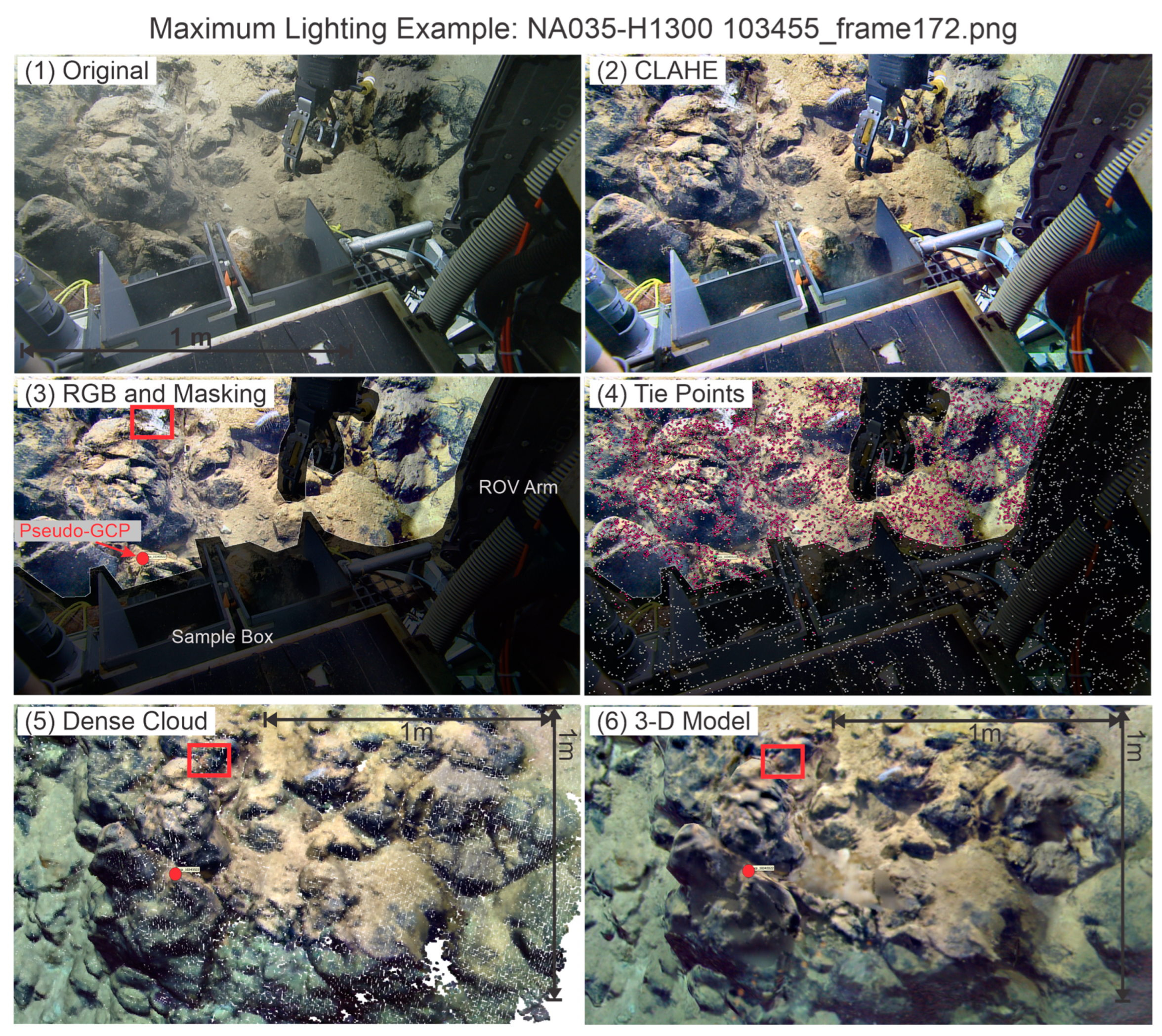
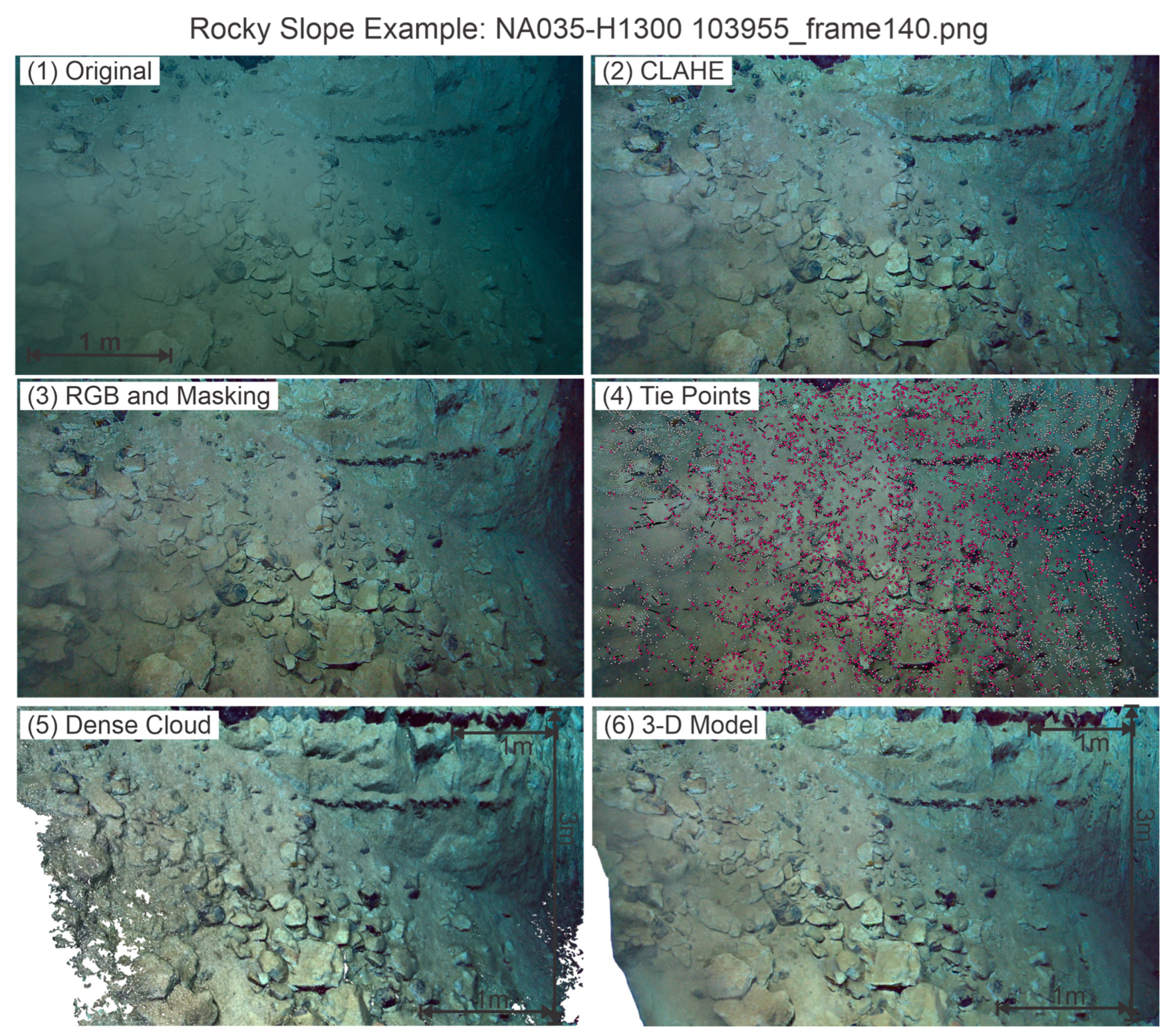
• Use masks to cover unwanted sections of images (example: edge of ROV).
• Align the images using photogrammetric software algorithms to obtain a tie point cloud.
• Convert the tie points and camera paths into a dense cloud which is the 3-D representation of the 3-D surface.
• From the dense cloud, export end products such as photomosaics or 3-D meshes with texture.
• Carry out scientific interpretation from these end products.

For a pre-planned project with the intent to use photogrammetry, sections of this workflow can be automated, can take advantage of super-computing facilities, and can be completed without significant human input. This is possible because pre-project planning will define optimal image collection paths [19] in step A to maximize the data available in the images that will later be used to align them in step C. When applying this workflow to data collected in an exploration mode or to archival decades-old data, we encounter problems in step C and are forced to provide human-guided input to complete this step, necessitating extra steps, or sub-steps, to be added between steps A and C.

There are limitations to converting ROV video collected in exploration mode into 3-D models using photogrammetry. These limitations stem from the deep-sea environment, the nature of the dives, and the requirements for imagery to be successfully processed using photogrammetry. Specific issues are listed as follows, and we attempt to address them in the next section (specific subsections in parentheses):

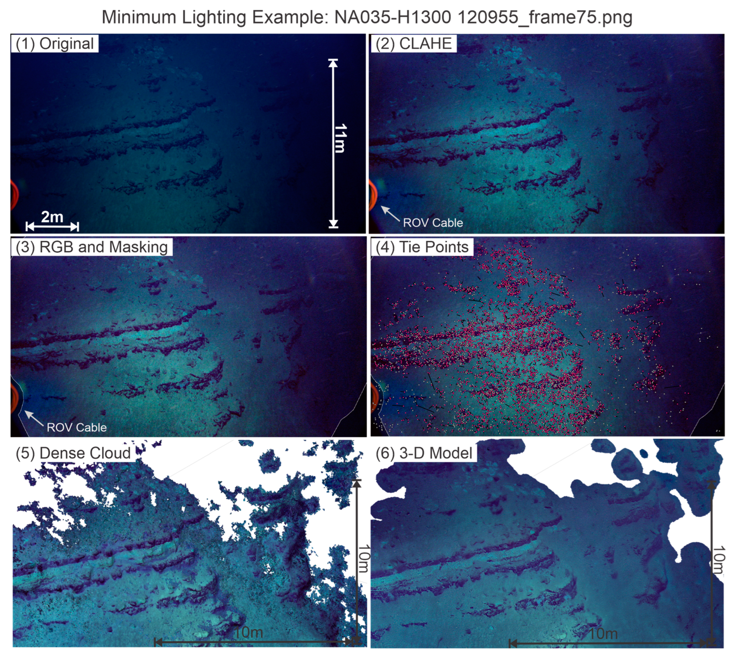
• Lighting: The distance that light can travel underwater is limited. In addition, light absorption by seawater is not uniform across the visible spectrum, and therefore, the color of an object is distorted by the distance from the camera lens. When objects are hard to make out because of insufficient lighting or because of turbid water, the photogrammetric process fails (Section 3.2).
• The ROV systems in the dives that we processed comprise two ROVs, one hovering over the other. While this configuration may help illuminate the seafloor, it may also add dark shadows that need to be masked in the images (Section 3.3).
• Travel paths: ROV paths do not follow a pre-planned grid pattern. They meander along a long and circuitous path from one point of interest to the next. As the ROV travels, it does not always maintain a constant speed and height above the seafloor. The height above the seafloor controls the resolution and the areal extent of ground captured in the image. Video sections cannot be used in photogrammetry when the ROV stops moving (Section 3.4 and Section 3.5).
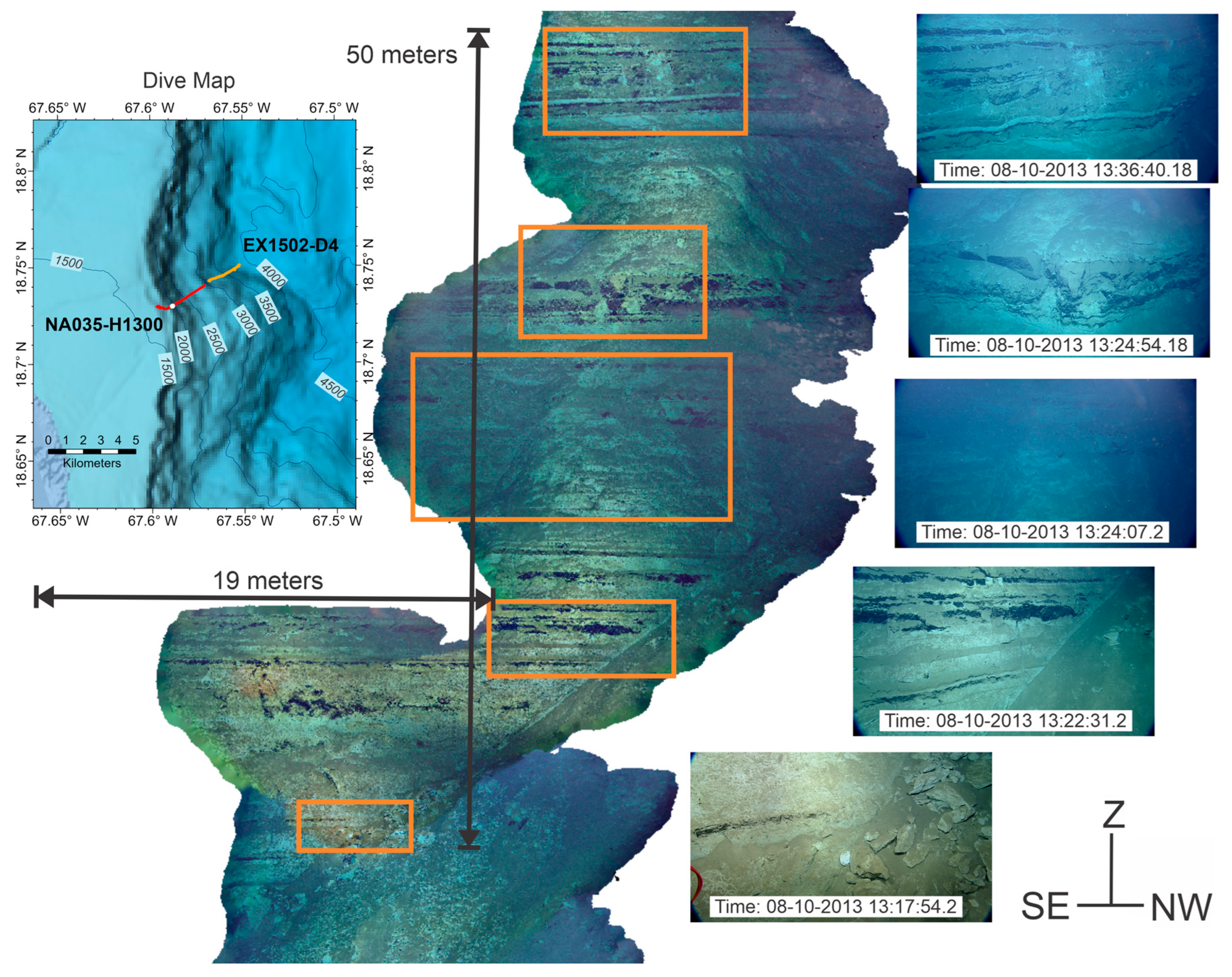
• Navigation: ROV navigation involves acoustic ranging between the ROV and the ship. Acoustic navigation has a limited depth resolution relative to electromagnetic ranging (e.g., GPS) and requires knowledge of sound speed in the seawater column [22]. ROV position was calculated via continuous acoustic ultra-short baseline (USBL) tracking [23]. The USBL position accuracy for the ROV Hercules at the time of data collection was 1° degree, or better than 2% of the slant range [24], which translates to an accuracy of a few tens of meters in deep-water dives. Unlike navigation in the terrestrial domain, the use of preexisting bathymetry for navigation is limited in the deep sea by its resolution (typically 10–25 m or more, depending on water depth) because the bathymetry has been collected by acoustic sounding from surface ships (Section 3.7).
• Ground control points (GCPs): Ground control points are not placed on the seafloor during an ROV traverse, limiting our ability to accurately georeference the photogrammetry products (Section 3.7).
• Camera orientation: Unlike a camera mounted on a drone where the camera angle is fixed with respect to the drone, the camera on the ROV moves up or down and from side to side independent of the ROV roll, pitch, and yaw, and this camera motion is not recorded. The camera may be at a 45° angle at the start of the dive and while the seafloor is flat, but it changes when the ROV is moving up along a steep incline or as the ROV is collecting and viewing objects of interest. The camera orientation is not a problem by itself, but it becomes an issue when combined with a change in the camera lens focal length reducing the overlap between images (Section 3.7).
• Camera lens focal length: Zooming with the HD camera is different from the ROV moving very close to an object because zooming changes the peripheral angle of view of the edges of the image. For photogrammetry software to work, there is a need to keep the apparent focal length of the camera lens as constant as possible, especially when the camera angle is moving (Section 3.4).
• Synchronizing the video data with the navigation: In our work, we have been using video that does not have EXIF (Exchangeable Image File Format) metadata embedded in the files. EXIF metadata can provide information on camera settings, date and time, and location. The only information we have is the frames-per-second rate of the video and the start time of the video, which is included in the file name (Section 3.7).

The two ROVs, Hercules and Deep Discoverer, are equipped with a pair of mounted lasers with a distance of 10 cm between them. Unfortunately, the lasers were turned on sparsely, but when they were present in the images, we used them to set the scale or check the distances on the photogrammetry products after georeferencing.

3. Results

The following photogrammetry workflow (

Table 1. Suggested workflow summary. Section refers to list of processes in main text.

Process (Step)	Software Used	Section	Process Summary
Image Generation and Preparation (A and B)	Metashape Professional v. 1.7 & 1.8	Section 3.1	Convert video stream to images at one-second increments. Each file should have a unique name and be based on the video file name.
	Python v. 3.8.5 & 3.8.12	Section 3.2	Generate an initial navigation file using the same one-second time increment to assign a unique navigation point for each image. Clean the images using the OpenCV CLAHE module.
	Metashape Professional v. 1.7 & 1.8	Section 3.3 and Section 3.4	Set up image groups and delete duplicate images and camera zoom-in sections. Mask unnecessary parts of images. Apply RGB color correction where needed. Apply brightness at 120%. Find pseudo-GCPs and mark them in the images. Add laser point references if available in any of the images and mark them.
Alignment: Build Tie Point Cloud (C)	Metashape Professional v. 1.7 & 1.8	Section 3.5 and Section 3.6	Apply alignment: If the software aligns successfully, continue to tie point cloud optimization. If the software fails to complete alignment, identify the reasons why the alignment of the image group failed. Continue with manually guided alignment to finish the alignment. Manually guided alignment: Based on the reason for alignment failure, guide the software to complete the alignment manually.
Georeference	Metashape Professional v. 1.7 & 1.8	Section 3.7	Synchronize the camera paths to the ROV navigation on a small section of the dive.
	Python v. 3.8.5 & 3.8.12	Section 3.7	Generate corrected camera navigation points for use in the rest of the dive.
	Microsoft Excel 2021	Section 3.7	Generate the pseudo-GCP X, Y, Z coordinates with the corrected camera navigation.
Tie Point Cloud Optimization	Metashape Professional v. 1.7 & 1.8	Section 3.8	Build hour-long camera sections from the smaller image groups. Remove outliers. Insert corrected camera navigation and pseudo-GCPs. Optimize camera paths based on navigation and pseudo-GCPs.
Build Dense Cloud (D)	Metashape Professional v. 1.7 & 1.8	Section 3.9	Remove outliers. Export and archive the dense cloud as .las or .laz files.
Build Products (E and F)	Metashape Professional v. 1.7 & 1.8	Section 3.10	Export and archive mesh as .obj files. Meshes should be no greater than 100,000 vertices to keep file size manageable.

) is expanded from the standard workflow outlined earlier and is designed to overcome the limitations and challenges in data acquisition from archival deep-sea video streams and those collected in exploration mode and the issues discussed earlier. Additional information is elaborated in the respective numbered sections below the table. Agisoft Metashape Professional © software [25] versions 1.7 and 1.8 (hereafter referred to as the photogrammetry software) is used here to carry out the photogrammetry. The proposed workflow can be adapted to other software because the outlined procedural steps are not tailored to specific software parameters. Unlike photogrammetry from terrestrial and pre-planned submarine surveys, navigation is added at a late stage of the workflow to improve the image-based alignment and for georeference. The workflow developed here uses the Over et al. [20] aerial imagery structure from motion and Hansman and Ring [21] terrestrial LIDAR survey workflows as a starting model.

3.1. Video Stream to Imagery

The expedition dive logs can be used to limit the scope of the video stream that needs to be processed, for example, targeting video streams that only focus on rock outcrops. In the photogrammetry software, we converted the five- to ten-minute cut sections of video streams, originally collected at 60 frames per second, into one-second increment images. The choice of a one-second increment is based on the speed of the ROVs. The ROVs in the processed dives moved at a median velocity of ~0.22 m/s over flat sections and at ~ 0.12 m/s over outcrop sections. Image overlap is also variable depending on the camera angle with respect to the imaged seafloor. The camera is not looking straight down, and consequently, the approximate area of the image is the bottom three-fourths of the image when the seafloor is flat (see Figure 3), but almost the entire image when the seafloor is almost vertical (see Figure 4, Figure 5 and Figure 6). A one-second increment was, therefore, a conservative value that significantly reduced the data volume while also satisfying the photogrammetry requirement of at least 60% and up to 70 to 90% overlap between images. In addition, images were edited out when the ROV was stationary or when the ROV camera was zooming into an object. Previous underwater photogrammetry also culled their video stream to increments of 1 [4] and 3 [2] seconds.

3.2. Digital Image Processing to Improve Image Quality

Lighting and the differential absorption of light underwater reduce the quality of the images as discussed in issue 1. Two components of the image must be addressed: contrast and color bias. Image processing techniques exist to address contrast in images and can be coded to apply individualized improvements to each image. Several algorithms can be deployed to edit underwater imagery with various levels of improvement; based on Mangeruda et al. [26] benchmarking different methods and testing their methods on the imagery, the Contrast Limited Adaptive Histogram Equalization (CLAHE) method is selected with the parameters of a tile size of 8 × 8 pixels and a contrast limit of 2. The open-source computer vision and machine learning software library known as OpenCV (version 4.0.1) (https://opencv.org/, accessed on 3 November 2022) [27] has the CLAHE module, and it is applied by writing a short script in Python (versions 3.8.5 and 3.8.12). As shown in Figure 3, Figure 4, Figure 5 and Figure 6, applying CLAHE improves the images and reveals objects and textures that otherwise would have been hidden without image processing. Instead of using the images in RGB (red–green–blue) color space, CLAHE is applied in YCbCr space, a common color space used for processing digital imagery. In this color space, Y is the luminance or the relative brilliance of the image, and Cb and Cr contain the color information, called chrominance. CLAHE isolates the luminance component of the images and modifies it separately from the color information. The images are then converted back to RGB color space for further processing in the photogrammetry software (See Appendix A for computing resources).

The CLAHE algorithm modifies some of the color bias seen in the original images. However, when the ROV is far from the seafloor and the target view area, the original image is mostly shades of blue, and the CLAHE algorithm struggles to modify the color despite improving the contrast (Figure 6). We further attempted to reduce the blue bias in the more distant images in the photogrammetry software, by shifting the percentage of green and blue color components based on the apparent distance to the seafloor from the ROV. This provided only modest improvement for seafloor images that are at the greatest distances from the ROV, but it significantly reduced the color bias in the intermediate distance range. The general rules of thumb for percent changes are listed in

Table 2. Corrections applied to balance the RGB color model.

	Rov Estimated Distance to Seafloor	Red	Green	Blue
(A)	Very close, inches to a couple of meters from the target. Sand has a tan color.	100%	100%	100%
(B)	Close, ~2–4 m, sand is a little tan but has some blue bias.	100%	95%	90%
(C)	Medium distance, ~4–8 m. All features in the image show a blue bias.	100%	90%	85%
(D)	Far distance, ~8–14 m. Everything in the image is in various shades of blue.	100%	85–80%	80–75%
(E)	Far away, ~>14 m. Everything in the image is dark blue.	100%	80%	70%

. In all cases, the red value was left unchanged at 100%. We increased the brightness to 110–120% on all the images. The modification of the RGB values can be a time-consuming process because the ROV does not keep a constant distance from the seafloor. That distance is not recorded digitally; therefore, the adjustment of RGB values is not constant and cannot be automated. This is also the most subjective part of the image-processing step.

3.3. Masking Unwanted Areas of the Images

Unwanted parts of images include the parts of the ROV that appear on the outer edges of the image (Figure 4 and Figure 6) and very dark shadows cast by the ROV from the second set of lights from the second ROV that hovers above the first ROV, as pointed out in issue 2. Other unwanted areas are objects in motion such as swimming fish, moving sea urchins, sediment clouds, and the ROV arm and cables, which appear in different spots between similar frames. Finally, bright spots of light, also known as lens flare, that appear from light sources captured within the image or from sharp reflections need to be masked too. If not masked, these unwanted areas in the image generate artifacts that appear in the later processing stages of the data such as the dense cloud, texture for the 3-D model, and orthomosaics. Our strategy is to manually generate several generalized mask shapes that can fit into many masking situations. For example, the bottom of the ROV may appear every time the camera is angled down to view an object or during sample collections (Figure 4), and a shape can be approximated to mask many images where this situation arises throughout the whole dive. The mask does not have to be perfect; it just needs to cover the unnecessary part of the image.

3.4. Building Image Groups and Editing out Unnecessary Images

Image groups of between 300 and 1500 images (5–25 min), or chunks in the photogrammetry software parlance, were created with the group size being a function of the desired machine processing time. Next, images where the ROV is stationary were edited out because photogrammetry processing requires actual motion from frame to frame. Sometimes, stationary sections are obvious, such as when the ROV is collecting a sample or when observing an object or an animal and involving camera zoom (issue 7). At other times, they are not obvious, such as when the ROV is hovering over the same spot with minimal rotation for several minutes while the ship operators are solving a technical problem or are running a calibration. Another situation that needs to be edited out is video frames where the ROV follows a moving point of interest, such as a swimming deep-sea octopus, and the ground cannot be seen in the background.

Editing out unwanted sections results in jumps in the continuity of the imagery (issue 3). If the ROV does not move or rotate, these jumps are small. However, photogrammetry algorithms typically fail when the ROV has very different positions and different perspectives before and after the cut section. The user will then have to manually identify points of reference between the gaps to guide the software and be able to merge the sections across the cut. At a minimum, four points of reference inside the images around the gaps or jumps should be used to help merge the sections together, but it is better to have between six and eight points. If no points can be found, then the endpoints of the cut section cannot be connected.

3.5. Running the Alignment

Unlike in pre-planned photogrammetry projects, navigation cannot be used to guide the process of alignment because of the navigation limitations in the deep sea, discussed earlier in issues 4 and 8. Instead, we rely on the quality of the images and use the slower but more reliable process of trying to match similar key features between images for the entire image group. Running the alignment process by strictly following the images in sequential order could be used to speed up the process, but it tends to fail in image groups that include gaps in continuity or where the ROV travels in a loop (resulting in features appearing again in a different angle) or rotates in place. Making the algorithm go through the entire image group to find matching points is the preferable method for catching these non-linear paths. These matching points collectively make up the cloud of tie points [20] along the camera path.

3.6. Continuing the Alignment Where It Failed

Alignment failures within image groups typically result from difficulty matching the key points between images rather than from a failure to identify key points in images. Only image groups with consistently excellent to good lighting, minimal continuity jumps, distinctive rock or seafloor textures, and a relatively stable and close distance of the ROV to the seafloor completed the alignment process without some form of human input.

The following solutions are suggested to overcome common failures of building the tie point cloud at the alignment stage:

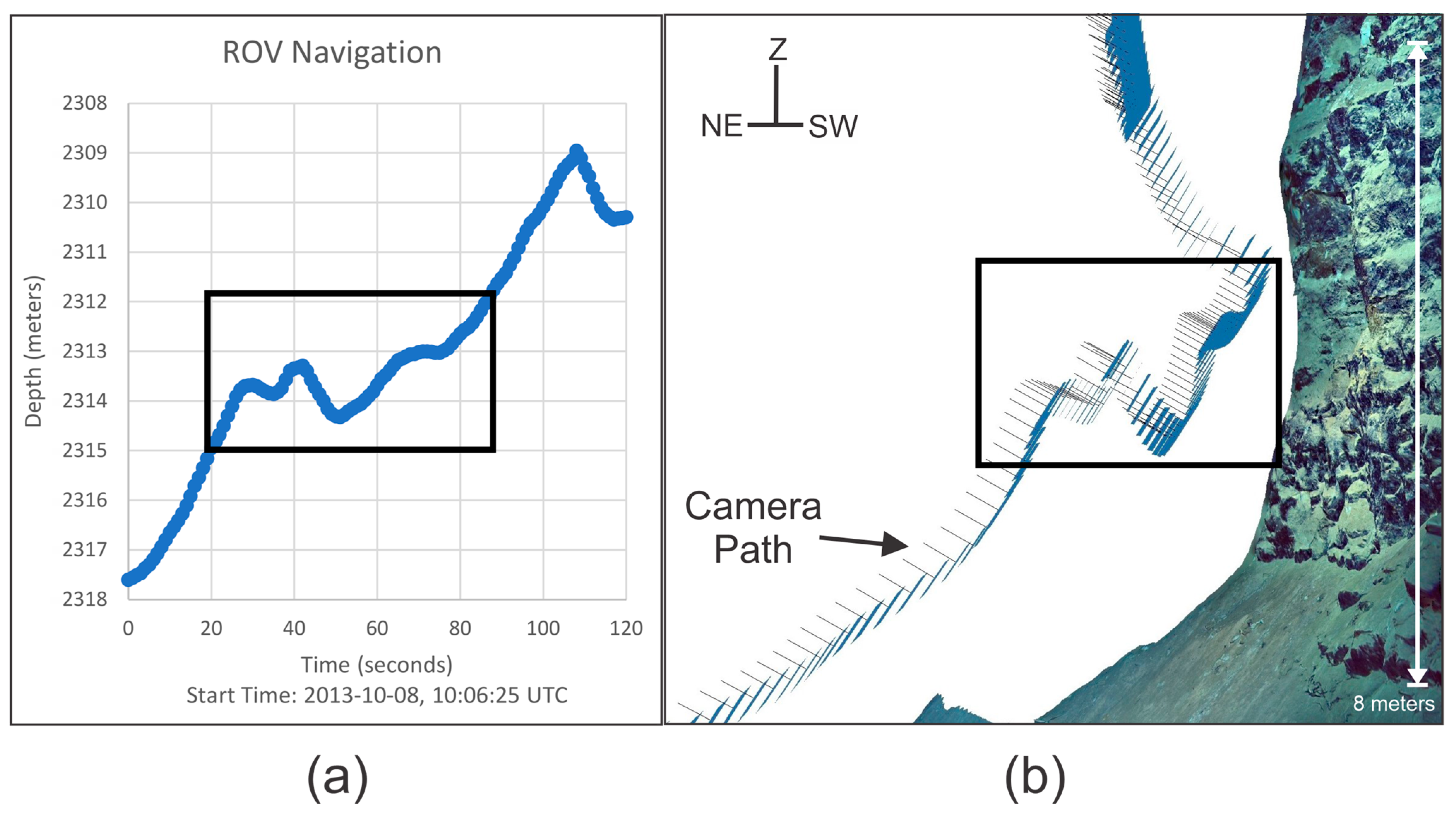
• Alignment often fails in sandy, featureless sections as shown in Figure 3. To resolve this issue, rebuild the camera path a few frames at a time until the image group is completed. There are usually enough points at the bottom two-thirds of the images to manually complete the alignment on the entire image group.
• Sometimes there is a continuity jump inside the image group that is too great for the software algorithm to match. In this situation, identify matching points or set up a minimum of four but preferably between six and eight markers or points to help guide the software to match up sections and continue the camera path.
• Turbid water blocks the view of the seafloor. These are the most difficult sections to align because the ROV is usually moving into or out of the sediment cloud, and points of reference are hard to find before and after these sediment clouds clear away. A section with a sediment cloud can be treated as a jump and processed as in item B above.
• When the focal length of the ROV camera changes when zooming in and out, the software applies one camera parameter where there should be two different camera parameters. To resolve this issue, points of reference need to be identified as in item B above and the section be treated as a continuity jump.
• Low lighting, even after improving the contrast, may impede the software’s ability to pick features to match (see Figure 6). It may be necessary to identify dark or light features and use them as markers to build a camera path, following the procedure in item B above. More than four points may be needed depending on how fast the ROV is moving. Once there is enough light in the images, the software can take over.
• Bad alignment solutions can show up as unconventional camera paths or tight spirals and can be the result of poor image overlap. The solution is to reset the camera alignment in those sections and rebuild the camera path a few frames at a time to fix the problem.

The remaining gaps in the camera path must be resolved by using the ROV navigation to help orient the edges of the gap. This is not an ideal situation and will be explained in more detail when adding the navigation. The alignment process step is the most time-consuming part of the entire workflow. Some outlier points in the tie point cloud may still need to be deleted after aligning every single image in the group.

3.7. Adding Navigation and Pseudo-GCPs and Calibrating the Camera Paths

Navigation is required to georeference the results of photogrammetry. The following two steps are required before adding the navigation to the photogrammetry results to resolve issue 8. First, the navigation needs to be synchronized with the camera path (see Figure 7) and second, navigation and camera orientation values need to be assigned to each image frame. Although the individual video frames are not time-stamped, the video file names include the start times. A time shift is required to synchronize the camera paths to the ROV navigation prior to assigning unique navigation values to each image frame. Depending on the quality of the ROV navigation, our assigned accuracy is between 10 m for the ROV Hercules data and 20 m for the ROV Deep Discoverer data.

The second piece of information to be combined with the navigation is the angle of the camera relative to the ROV. We assigned an assumed angle of 65° plus the pitch from the gyroscope of the ROV to resolve issue 6. The value of 65° seems to be the median between the camera angle used on a flat seafloor (45°) and when the ROV is moving up along a vertical slope (85°). The yaw, pitch, and roll of the ROV are important components in setting the orientation of the photogrammetry results. We assign an error range of 20° to account for the unknown angle changes the camera makes relative to the ROV during the dive.

In the absence of surveyed seafloor markers that can serve as ground control points (GCP), we define pseudo-GCPs along the dive path to resolve issue 5. A pseudo-GCP is any point in the dive where the ROV has touched the seafloor and stayed in place for a minimum of 15 s or when the ROV is hovering less than about 0.10 m above the bottom for around 20 s or more. In these locations, we can time-average repeated longitude, latitude, and depth determinations by the USBL to get a better true location of the ROV than during continuous movement. The most reliable points are those where the ROV has touched the ground to collect a sample and the front bottom edge of the ROV can be observed. Inside the images, a reference point needs to be identified and placed as close to the approximate location of the front-center-bottom edge of the ROV (see Figure 4, red dot). An X and Y accuracy of 1.0 m is assigned for all points. For the Z accuracy, 0.01 m is assigned if the ROV touched the ground, and 0.10 m is assigned when the ROV hovered very close to the ground.

The ROV lasers can also help scale the photogrammetry results. This is especially helpful when no pseudo-GCPs are found within a section of the dive. The set distance between the laser points is 0.10 m for both ROVs in our study with an accuracy of 0.001 m [28]. The laser points must be projected onto a flat surface to derive an accurate measurement.

3.8. Merging Image Groups and Optimization

Merging the image groups (Section 3.4) requires six to eight points in common at the edges of the image sections. Unique names or labels should be given to the reference points when merging these image sections together. With our computer resources, we stitched together one-hour-long sections that included between 2000 and 3600 images. The camera paths need to be adjusted to minimize misfits between images. After merging sections together, a camera calibration is applied to reduce the RMS (root mean squared) errors of the X, Y, and Z camera paths and pseudo-GCPs [25]. The calibration process in other photogrammetric software may have a similar procedure to help reduce the RMS error of several variables (X, Y, Z location; orientation angles; and pixel reprojection errors) in the tie point cloud. At a minimum, the camera calibration should be performed once after editing out tie point outliers to achieve the best results. Good RMS errors are those falling within the assigned accuracy values [20,25].

3.9. Building the Dense Cloud from the Tie Points

Tie points come from searching for features inside each image and then matching them across all the images. The dense cloud uses the tie points and the camera parameters, path, and orientations to populate a 3-D cloud of points, each point being triangulated from every pair of images [25]. The tie point model should be inspected for any mismatch between image sections, and outliers should be removed before building the dense cloud. Outliers are distant points on the outer edges of the cloud of tie points that seem off-angle or not in line with the main tie points. Mismatches can be fixed by adding reference points and then running the optimization step again. There is no need to return to the alignment step.

Depending on the user’s research goals, the dense cloud (see examples in Figure 3, Figure 4, Figure 5 and Figure 6) may be the final product and the end of the workflow. Pieces of software, such as CloudCompare [29], can be used to process the dense cloud for further analysis outside of the photogrammetry software. Potree [30] is another point cloud viewer. The dense cloud can also be an archivable product if saved like LIDAR data in .las or .laz file formats. The user is directed to the Open Topography project (https://opentopography.org/, accessed on 3 November 2022) for suggested settings and meta-file requirements for later archiving and if they opt to deposit their projects there.

3.10. Converting the Dense Cloud into Other Viewable Products for Collaboration

Our goal was to generate a product that is detailed at the almost centimeter-scale resolution but has a file size of only a few hundred MB so it can be used in scientific collaborations. The file size of an hour-long dense cloud section (several hundreds of MB to one GB) makes sharing and manipulating the results cumbersome. Our solution was to convert the dense cloud into a textured 3-D mesh and export the .obj file, at less than 100 MB, into another piece of software for geologic interpretation (see 3-D model examples in Figure 3, Figure 4, Figure 5 and Figure 6). By limiting the number of vertices to a maximum of 1,000,000 but still applying detailed texture, we can generate a product that can be shared by desktop and laptop computers. The optimal number of vertices for the mesh is around 750,000 with an image texture by size count of 4096 × 10. It is also preferable to export the project into UTM coordinates to make it easier to measure distances in meters. Software options for geologic interpretation include LIME © [31] and Sketchfab, Inc., New York, NY, USA (https://sketchfab.com/, accessed on 13 February 2023), which uses an external website to host 3-D models, and gaming software for developing a virtual 3-D experience [32].

4. Discussion

4.1. Reliance on Image Quality Instead of Navigation to Build the Model

The final photogrammetry model relied heavily on high-resolution imagery instead of the known navigation of the ROV. Our initial attempts at using navigation to help align the images resulted in failures despite assigning a large navigational accuracy of 20 m. The photogrammetry process was more successful when we added the navigation after the alignment because the overlapping high-resolution imagery was more effective at determining the path of the ROV than the provided navigation data (see Figure 7). With at least three evenly distributed pseudo-GCPs in the image section, it is possible to back-calculate the ROV navigation path.

4.2. True Color of Objects Underwater

Color is distorted in underwater imagery by the differential attenuation of the visible-frequency spectrum by seawater. The ideal way to obtain the true color of an image taken underwater would be to have a series of reference objects with known color values at various measured distances from the camera lens to help correct the color balance [33]. In shallow water, this could be a reference plate with black and white patterns, a diver’s breathing tank, or some other object brought from the surface that is a neutral color of white, black, or grey.

The ROV arm is painted with reference color marks that are used to color balance the video (see Figure 1 bottom-left area circled with red oval); however, the arm is located only about a meter away from the camera lens. The two-ROV configuration used during the dive also introduced an additional problem of having two light sources with varying positions and distances to the sea floor. The lack of reference objects that can be used at set distances from the camera makes it impossible to carry out color balance correction at known distances from the camera in these deep-sea environments. Although we cannot assess the true color, we can obtain relative contrasts between light- and dark-colored features and distinguish rocks that are dark versus those that are in a shadow. We can also interpret features based on their texture, slope angle, direction of joints, and alignment of debris.

4.3. Suggested Improvements to ROV Operations in Deep Water

Significant improvements in the use of ROV video streams for quantitative analysis can be achieved with modest modifications to data recording, ROV operation, and equipment. The alignment procedure would be improved with a continuous timestamp in the video frames to help synchronization with the navigation timestamp. A record of the camera position and angle relative to the ROV would also assist the photogrammetry and allow for a reliable extraction of geologic dips.

ROV operation in an exploration mode could be improved to help build the model as follows:

(a)

More reference points are needed to improve the navigation. Because it is impractical to place markers on the sea floor, we generated pseudo-GCP markers by having the ROV rest on the seafloor or hover in place for at least 15 s but preferably for 60 s and averaging the X, Y, and Z coordinate reading. Pseudo-GCPs should preferably be collected every 15 min along the transect.

(b)

Flying through sediment clouds should be avoided because the accuracy of the navigation is not sufficient to piece together sections across the sediment cloud. It is preferable to wait until the sediment settles and visibility improves before moving again.

(c)

When chasing fish and other deep-sea fauna, the ROV should return to a reference feature to create a “continuous” video.

The extraction of the real colors of the seafloor can be achieved by installing a high-frequency sonar to measure the distance from the camera to the filmed object. Absent this capability, the ROV lasers should be turned on more often and for at least 10 s to illuminate the target seafloor. In addition, the ROV arm can place a colored calibration plate on the seafloor below the photic zone and slowly move away from the plate while measuring its distance from the camera.

4.4. Building a Project for a Visiting Summer Student

Currently, there is a vast depository of ROV videos hosted by academic institutions in the USA and abroad and by the Ocean Exploration Trust and NOAA Ocean Exploration. The impetus for his project was only concerned with one area of the seafloor, the Mona Rift, Puerto Rico. We recruited two Woods Hole Oceanographic Institution Summer Student Fellows working on two separate dives, and they presented their results at the American Geophysical Union Fall meetings [34,35] and were co-authors on a scientific paper [17]. Having a student work on a dive involved planning and setting up both resources and software before the start of the project. Part of this advanced planning included developing the scripts in Python to modify the images using CLAHE and manipulate the ROV navigation to fit the one-second increments of the dive video imagery before the students arrived. It was helpful to the authors to obtain feedback from the students on what worked or did not work while processing the dives. It also helped the students to have a pre-defined goal to help focus the project in the short time allotted. Based on the feedback from the students, we realized that applying photogrammetry to archived ROV HD videos can serve as an excellent educational tool.

4.5. Measurable Results

The Mona Rift shown in Figure 1 has been extensively studied using other remote sensing methods such as sidescan sonar [36], multibeam bathymetry [12], multichannel seismic reflection data [37], and earthquake locations [6,8]. The addition of photogrammetry data to this older collection provides an additional and unique aspect to the understanding of the earthquake, tsunami, and submarine landslide hazards in this area. Ten Brink et al. [17] used the photogrammetric image from a several-kilometer-long dive to deduce the origin of the devastating 1918 earthquake and tsunami (outlined in yellow in Figure 1). Their insight was guided by the results of the 3-D photogrammetric model of dive NA035-H1301 and the associated dated rock samples. Prior publications based on multibeam and seismic reflection data [10,11] placed the origin of the 1918 tsunami in a giant landslide scar [17]. However, the dives in the area showed the landslide scar to be older than 1918 and identified a fault plane responsible for the earthquake and the tsunami.

A 2400 m high segment of Mona Rift wall was mapped as a virtual geological outcrop by applying our workflow to two ROV dives (outlined in red in Figure 2 inset) and was compared to deep boreholes and surface geology on land in Puerto Rico [18]. This comparison allowed the authors to extend the geology on land to over 100 km offshore and interpret the rifting history of Mona Rift. A more complete and interpreted section shown in Figure 2 is shown and discussed in detail in the work of ten Brink et al. [18].

5. Conclusions

The wealth of available video streams from archives of deep-sea manned, unmanned, and tow-camera explorations can become more scientifically useful by extracting quantifiable information with the aid of photogrammetry (e.g., ten Brink et al. [17]). Standard photogrammetry procedures developed for aerial drone surveys and for pre-planned submarine surveys cannot be applied to these deep-sea video data because the ROV path is a single non-linear path and includes variable viewpoints of the target area. Additional complicating factors include poor navigation, variable lighting, variable distance from the seafloor, variable speed of the ROV, and variable camera orientation with respect to the ROV. In particular, the lack of accurate navigation necessitates reliance on image quality and the establishment of pseudo-ground-control points to build a 3-D model. We developed a workflow for processing archival video data collected at water depths of 1000–4000 m in the vicinity of Puerto Rico collected by two separate ROV systems on four separate dives. This workflow allows a quantitative exploration of the deep-sea environment, adding context to the images and the possibility of making physical measurements of objects or geologic features observed in the videos. Although the workflow requires significantly more human interaction with the data, our training of undergraduate summer students shows that the workflow is easily learned, and a dive can be processed within a few months.

References

1. Abdelaziz, M.; Elsayed, M. Underwater Photogrammetry Digital Surface Model (DSM) of the Submerged Site of the Ancient Lighthouse near Qaitbay Fort in Alexandria, Egypt. Int. Arch. Photogramm. Remote Sens. Spat. Inf. Sci. 2019, XLII-2/W10, 1–8. [Google Scholar] [CrossRef]
2. Boittiaux, C.; Dune, C.; Ferrera, M.; Arnaubec, A.; Marxer, R.; Matabos, M.; Van Audenhaege, L.; Hugel, V. Eiffel Tower: A Deep-Sea Underwater Dataset for Long-Term Visual Localization. Int. J. Robot. Res. 2023, 42, 689–699. [Google Scholar] [CrossRef]
3. Barreyre, T.; Escartín, J.; Garcia, R.; Cannat, M.; Mittelstaedt, E.; Prados, R. Structure, Temporal Evolution, and Heat Flux Estimates from the Lucky Strike Deep-sea Hydrothermal Field Derived from Seafloor Image Mosaics. Geochem. Geophys. Geosystems 2012, 13, 2011GC003990. [Google Scholar] [CrossRef]
4. Price, D.M.; Robert, K.; Callaway, A.; Lo Lacono, C.; Hall, R.A.; Huvenne, V.A.I. Using 3D Photogrammetry from ROV Video to Quantify Cold-Water Coral Reef Structural Complexity and Investigate Its Influence on Biodiversity and Community Assemblage. Coral Reefs 2019, 38, 1007–1021. [Google Scholar] [CrossRef]
5. Escartín, J.; Leclerc, F.; Olive, J.-A.; Mevel, C.; Cannat, M.; Petersen, S.; Augustin, N.; Feuillet, N.; Deplus, C.; Bezos, A.; et al. First Direct Observation of Coseismic Slip and Seafloor Rupture along a Submarine Normal Fault and Implications for Fault Slip History. Earth Planet. Sci. Lett. 2016, 450, 96–107. [Google Scholar] [CrossRef]
6. Reid, H.F.; Taber, S. The Porto Rico Earthquakes of October-November, 1918. Bull. Seismol. Soc. Am. 1919, 9, 95–127. [Google Scholar] [CrossRef]
7. Mercado, A.; McCann, W. Numerical Simulation of the 1918 Puerto Rico Tsunami. Nat. Hazards 1998, 18, 57–76. [Google Scholar] [CrossRef]
8. Doser, D.I.; Rodriguez, C.M.; Flores, C. Historical Earthquakes of the Puerto Rico–Virgin Islands Region (1915–1963). In Active Tectonics and Seismic Hazards of Puerto Rico, the Virgin Islands, and Offshore Areas; Mann, P., Ed.; Geological Society of America: Boulder, CO, USA, 2005; Volume 385, ISBN 978-0-8137-2385-3. [Google Scholar] [CrossRef]
9. Hornbach, M.J.; Mondziel, S.A.; Grindlay, N.; Frohlich, C.; Mann, P. Did a Submarine Slide Trigger the 1918 Puerto Rico Tsunami? Sci. Tsunami Hazards 2008, 27, 22–31. [Google Scholar]
10. López-Venegas, A.M.; Ten Brink, U.S.; Geist, E.L. Submarine Landslide as the Source for the October 11, 1918 Mona Passage Tsunami: Observations and Modeling. Mar. Geol. 2008, 254, 35–46. [Google Scholar] [CrossRef]
11. López-Venegas, A.M.; Horrillo, J.; Pampell-Manis, A.; Huérfano, V.; Mercado, A. Advanced Tsunami Numerical Simulations and Energy Considerations by Use of 3D–2D Coupled Models: The October 11, 1918, Mona Passage Tsunami. Pure Appl. Geophys. 2015, 172, 1679–1698. [Google Scholar] [CrossRef]
12. Andrews, B.D.; ten Brink, U.S.; Danforth, W.W.; Chaytor, J.D.; Granja-Bruna, J.; Carbo-Gorosabel, A. Bathymetric Terrain Model of the Puerto Rico Trench and the Northeastern Caribbean Region for Marine Geological Investigations; U.S. Geological Survey: Reston, Virginia, 2014; p. 1. [Google Scholar] [CrossRef]
13. ten Brink, U.S.; Coleman, D.F.; Chaytor, J.; Demopoulos, A.W.J.; Armstrong, R.; Garcia-Moliner, G.; Raineault, N.; Andrews, B.; Chastain, R.; Rodrigue, K.; et al. Earthquake, Landslide, and Tsunami Hazards and Benthic Biology in the Greater Antilles. Oceanography 2014, 27, 34–35. [Google Scholar]
14. Kennedy, B.R.C.; Cantwell, K.; Sowers, D.; Cheadle, M.J.; McKenna, L.A. EX1502 Leg 3, Océano Profundo 2015: Exploring Puerto Rico’s Seamounts, Trenches, and Troughs: Expedition Report; U.S. National Oceanic and Atmospheric Administration, Office of Ocean Exploration and Research: Silver Spring, MD, USA, 2015. [Google Scholar] [CrossRef]
15. Mondziel, S.; Grindlay, N.; Mann, P.; Escalona, A.; Abrams, L. Morphology, Structure, and Tectonic Evolution of the Mona Canyon (Northern Mona Passage) from Multibeam Bathymetry, Side-Scan Sonar, and Seismic Reflection Profiles: Mona canyon tectonics. Tectonics 2010, 29, TC2003. [Google Scholar] [CrossRef]
16. ten Brink, U.; Danforth, W.; Polloni, C.; Andrews, B.; Llanes, P.; Smith, S.; Parker, E.; Uozumi, T. New Seafloor Map of the Puerto Rico Trench Helps Assess Earthquake and Tsunami Hazards. Eos Trans. Am. Geophys. Union 2004, 85, 349–354. [Google Scholar] [CrossRef]
17. ten Brink, U.; Chaytor, J.; Flores, C.; Wei, Y.; Detmer, S.; Lucas, L.; Andrews, B.; Georgiopoulou, A. Seafloor Observations Eliminate a Landslide as the Source of the 1918 Puerto Rico Tsunami. Bull. Seismol. Soc. Am. 2023, 113, 268–280. [Google Scholar] [CrossRef]
18. ten Brink, U.S.; Bialik, O.M.; Chaytor, J.D.; Flores, C.H.; Philips, M.P. Field Geology under the Sea with a Remotely Operated Vehicle: Mona Rift, Puerto Rico. Geosphere 2024. submitted. Available online: https://eartharxiv.org/repository/view/6838/ (accessed on 19 July 2024).
19. Arnaubec, A.; Ferrera, M.; Escartín, J.; Matabos, M.; Gracias, N.; Opderbecke, J. Underwater 3D Reconstruction from Video or Still Imagery: Matisse and 3DMetrics Processing and Exploitation Software. J. Mar. Sci. Eng. 2023, 11, 985. [Google Scholar] [CrossRef]
20. Over, J.-S.R.; Ritchie, A.C.; Kranenburg, C.J.; Brown, J.A.; Buscombe, D.D.; Noble, T.; Sherwood, C.R.; Warrick, J.A.; Wernette, P.A. Processing Coastal Imagery with Agisoft Metashape Professional Edition, Version 1.6—Structure from Motion Workflow Documentation; U.S. Geological Survey: Reston, Virginia, 2021. [Google Scholar] [CrossRef]
21. Hansman, R.J.; Ring, U. Workflow: From Photo-Based 3-D Reconstruction of Remotely Piloted Aircraft Images to a 3-D Geological Model. Geosphere 2019, 15, 1393–1408. [Google Scholar] [CrossRef]
22. Blain, M.; Lemieux, S.; Houde, R. Implementation of a ROV Navigation System Using Acoustic/Doppler Sensors and Kalman Filtering. In Proceedings of the Oceans 2003. Celebrating the Past... Teaming Toward the Future (IEEE Cat. No.03CH37492), San Diego, CA, USA, 22–26 September 2003; Volume 3, pp. 1255–1260. [Google Scholar]
23. Zieliński, A.; Zhou, L. Precision Acoustic Navigation for Remotely Operated Vehicles (ROV). Hydroacoustics 2005, 8, 255–264. [Google Scholar]
24. Bell, K.L.C.; Brennan, M.L.; Raineault, N.A. New Frontiers in Ocean Exploration: The E/V Nautilus 2013 Gulf of Mexico and Caribbean Field Season. Oceanography 2014, 27, 52. [Google Scholar] [CrossRef]
25. Agisoft Metashape: Agisoft Metashape. Available online: https://www.agisoft.com/ (accessed on 22 February 2024).
26. Mangeruga, M.; Bruno, F.; Cozza, M.; Agrafiotis, P.; Skarlatos, D. Guidelines for Underwater Image Enhancement Based on Benchmarking of Different Methods. Remote Sens. 2018, 10, 1652. [Google Scholar] [CrossRef]
27. OpenCV. Available online: https://opencv.org/ (accessed on 2 April 2024).
28. Istenič, K.; Gracias, N.; Arnaubec, A.; Escartín, J.; Garcia, R. Scale Accuracy Evaluation of Image-Based 3D Reconstruction Strategies Using Laser Photogrammetry. Remote Sens. 2019, 11, 2093. [Google Scholar] [CrossRef]
29. CloudCompare—Open Source Project. Available online: https://www.cloudcompare.org/ (accessed on 22 February 2024).
30. Schütz, M. Potree: Rendering Large Point Clouds in Web Browsers. Master’s Thesis, Technische Universität Wien, Vienna, Austria, 2015. [Google Scholar]
31. Buckley, S.J.; Ringdal, K.; Naumann, N.; Dolva, B.; Kurz, T.H.; Howell, J.A.; Dewez, T.J.B. LIME: Software for 3-D Visualization, Interpretation, and Communication of Virtual Geoscience Models. Geosphere 2019, 15, 222–235. [Google Scholar] [CrossRef]
32. Needle, M.D.; Mooc, J.; Akers, J.F.; Crider, J.G. The Structural Geology Query Toolkit for Digital 3D Models: Design Custom Immersive Virtual Field Experiences. J. Struct. Geol. 2022, 163, 104710. [Google Scholar] [CrossRef]
33. Akkaynak, D.; Treibitz, T. Sea-Thru: A Method for Removing Water From Underwater Images. In Proceedings of the 2019 IEEE/CVF Conference on Computer Vision and Pattern Recognition (CVPR), Long Beach, CA, USA, 15–20 June 2019; pp. 1682–1691. [Google Scholar] [CrossRef]
34. Detmer, S.; ten Brink, U.S.; Flores, C.H.; Chaytor, J.D.; Coleman, D.F. High Resolution 3D Geological Mapping Using Structure-from-Motion Photogrammetry in the Deep Ocean Bathyal Zone. In Proceedings of the AGU Fall Meeting 2021, New Orleans, LA, USA, 15 December 2021. [Google Scholar]
35. Lucas, L.C.; ten Brink, U.S.; Flores, C.H.; Chaytor, J.D. Geological Mapping in the Deep Ocean Using Structure-from-Motion Photogrammetry. In Proceedings of the AGU Fall Meeting 2022, Chicago, IL, USA, 12 December 2022. [Google Scholar]
36. Paskevich, V.F.; Wong, F.L.; O’Malley, J.J.; Stevenson, A.J.; Gutmacher, C.E. GLORIA Sidescan-Sonar Imagery for Parts of the U.S. Exclusive Economic Zone and Adjacent Areas; U.S. Geological Survey: Reston, VA, USA, 2011. [Google Scholar] [CrossRef]
37. Triezenberg, P.J.; Hart, P.J.; Childs, J.R. National Archive of Marine Seismic Surveys (NAMSS: A USGS Data Website of Marine Seismic Reflection Data within the U.S. Exclusive Economic Zone (EEZ). 2016. Available online: https://www.usgs.gov/data/national-archive-marine-seismic-surveys-namss-a-usgs-data-website-marine-seismic-reflection (accessed on 22 February 2024). [CrossRef]
Figure 1. (Top): Map of dives labeled and shown in red and orange located near the Mona Rift, northwest of Puerto Rico. Contours show depths in meters at 500 m intervals. Square indicates location of dive map shown in Figure 2. Bathymetry from Andrews et al. [12]. Yellow curve denotes landslide tsunami source of Lopéz-Venegas et al. [10,11]. Large and small white stars denote proposed epicenter of the October 10, 1918, M 7.2 earthquake and aftershocks (International Seismological Center Global Earthquake Model [ISC-GEMS] catalog). Inset: General map of the Northeastern Caribbean showing Haiti, Dominican Republic, and Puerto Rico. (Bottom left) Photo of the front of ROV Hercules. The red rectangle indicates the location of the video camera on the ROV. The red oval indicates the location of the ROV arm, used to grab rock samples and push sediment cores. Color reference marks on the arm are used to color balance the video, but note the proximity of the marks to the camera. Image Credit: Mark Deroche, Ocean Exploration Trust. Image was cropped from the original to focus on the ROV. (Bottom right) Photo of the front of the ROV Deep Discoverer. The red rectangle shows the location of the video camera. Image Credit: Art Howard, GFOE-Global Foundation for Ocean Exploration, Windows of the Deep 2018. Image has been cropped from the original to focus on the ROV.
Jmse 12 01250 g001
Figure 2. (Main Image)—Small section of Hercules Dive NA035-H1300 northwest of Puerto Rico at a depth interval of 1918 to 1876 m shown as white dot in the dive map. The perspective is looking towards the southwest and depth is vertical. Arrows indicate distance measurements for the section. Individual video images on the right correspond to the orange rectangles on the section. The size of the rectangle corresponds to the field of view shown in the image. Images are taken from the ROV dive video and have not been image processed. The time stamps in the images are from the navigation. (Inset)—Map showing some dive locations in Western Mona Rift. Location of map is shown in Figure 1. Bathymetry is from Andrews et al. [12].Contours are shown and labeled as depths in meters.
Jmse 12 01250 g002
Figure 3. A frame of a flat and sandy seafloor taken from Dive NA035-H1301 at time stamp 09-10-2013 03:49:56.14 UTC at a depth of −1972 m (18.48180681, −67.32770409). Note the difference in horizontal distance between the top and bottom of the image because of the slant angle of the camera. The six images show the processing progression: (1) the original image taken from the ROV HD video; (2) applying CLAHE to the image; (3) bringing the image back into the photogrammetry software to adjust the RGB values (100:90:85), adding a mask to cover the edge of the camera lens at the four corners of the image and adjusting the brightness (ROV shadows are indicated by arrows); (4) showing the tie points, in magenta, found by the software that were matched with at least one other image in the sequence; (5) a section of the dense cloud at the same approximate scale and perspective as the original image; and (6) a section of the 3-D model at the same approximate scale and perspective as the original image. The lack of an ROV shadow in images (5,6) is because these sections are the result of combining overlapping images in the sequence.
Jmse 12 01250 g003
Figure 4. Maximum lighting example taken from Dive NA035-H1300 at time stamp 08-10-2013 10:37:17.22 UTC and navigation location of (18.7319671, −67.5844621) at a depth of −2231 m. Each of the six images shows the progression of (1) the original image taken from the ROV HD video; (2) applying CLAHE to the image; (3) bringing the image back into the photogrammetry software to adjust the RGB values (100:95:90), adding a mask to cover the ROV arm and sample box, and adjusting the brightness; (4) showing the tie points, in magenta, found by the software that were matched with at least one other image in the sequence; (5) a section of the dense cloud at approximate scale and perspective as the original image; and (6) a section of the 3-D model at approximate scale and perspective as the original image. Images (3,5,6) indicate the pseudo-GCP with a red dot. The red box shows the location of the rock sample, NA035-030, being picked by the mechanical arm in image (3). The rock sample location is indicated by the same red box in the dense cloud (5) and 3-D model (6). The lower part of the image hidden by the ROV in images (14) is revealed in images (5,6) by combining overlapping images in the sequence.
Jmse 12 01250 g004
Figure 5. Rocky slope example taken from Dive NA035-H1300 at time stamp 08-10-2013 10:41:45.22 UTC and navigation location of (18.73187265, −67.58452751) at a depth of −2222 m. Each of the six images shows the progression of (1) the original image taken from the ROV HD video; (2) applying CLAHE to the image; (3) bringing the image back into the photogrammetry software to adjust the RGB values (100:90:85) and the brightness; (4) showing the tie points, in magenta, found by the software that were matched with at least one other image in the sequence; (5) a section of the dense cloud at the same approximate scale and perspective as the original image; and (6) a section of the 3-D model at the same approximate scale and perspective as the original image. The lower left corner of the original image shows a sediment cloud that contributes to the paucity of data that can be retrieved from that part of the image as shown in images (46).
Jmse 12 01250 g005
Figure 6. Minimum lighting example taken from Dive NA035-H1300 at time stamp 08-10-2013 12:10:40.04 UTC and navigation location of (18.73083431, −67.58661955) at a depth of −2046 m. Each of the six images shows the progression of (1) the original image taken from the ROV HD video; (2) applying CLAHE to the image; (3) bringing the image back into the photogrammetry software to adjust the RGB values (100:85:75), adding a mask for the red cable from the arm of the ROV indicated by the arrow, and adjusting the brightness; (4) showing the tie points, in magenta, found by the software that were matched with at least one other image in the sequence; (5) a section of the dense cloud at the same approximate scale and perspective as the original image; and (6) a section of the 3-D model at the same approximate scale and perspective as the original image.
Jmse 12 01250 g006
Figure 7. (a) A plot of time versus depth from the ROV navigation. The black rectangle outlines a pattern in the ROV navigation (b) Screen shot from the photogrammetry software showing a partial image of the base of the vertical outcrop at a depth of ~2315 m in Dive NA035-H1300. The corresponding camera path is indicated as blue squares representing each image used to build the 3-D model section, and the thin lines are their back projection to the ROV. The camera path was developed independently from the navigation by stitching the overlapping video frames. Both the image and the camera path are rotated in 3-D. The orientation indicated by the axis at the top-left is after geo-referencing the 3-D model. The black rectangle in (b) shows that the camera path pattern is similar to the navigation pattern outlined in (a) despite being derived independently.
Jmse 12 01250 g007