
Failure Consequence Cost Analysis of Wave Energy Converters—Component Failures, Site Impacts, and Maintenance Interval Scenarios

 , , ,
, , ,  , ,
, ,  and
and
Abstract
1. Introduction
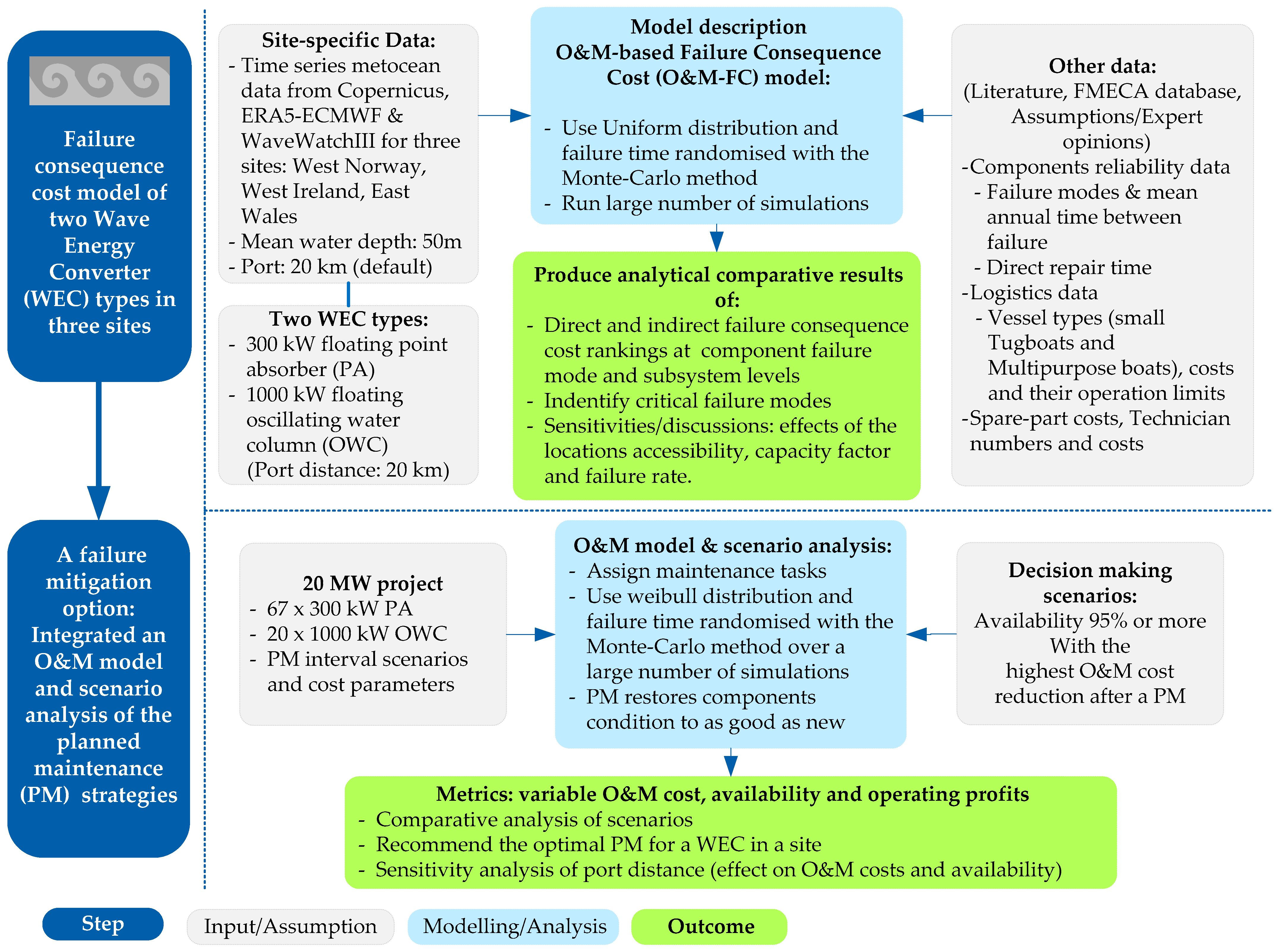
2. Method
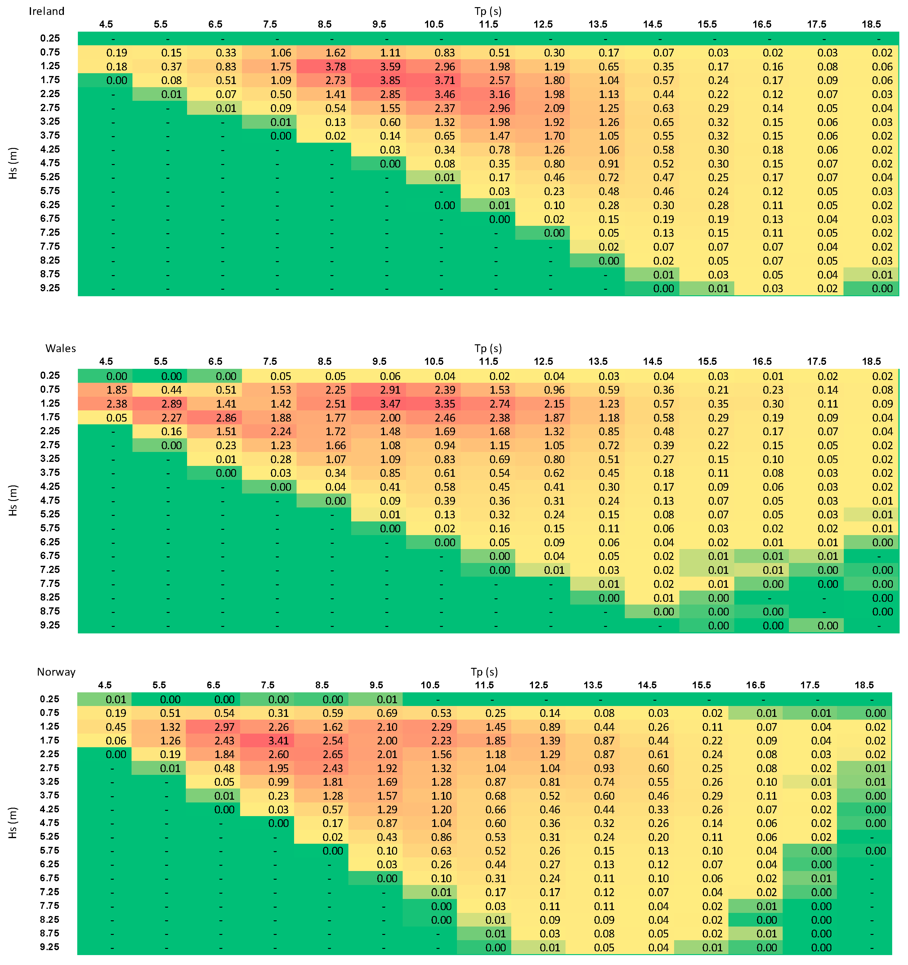
2.1. Time Series Metocean Data
2.2. WECs
2.3. Power Matrix and Potential Power Production
2.4. Failure and Repair Data
- The biggest information source for these data is gathered from the generic WEC FMECA database [56] for the IMPACT project (https://www.impact-h2020.eu/, accessed on 10 May 2024). The database in [56] is primarily obtained from the Offshore & Onshore Reliability Data (OREDA@Cloud) (https://store.veracity.com/oreda-cloud-offshore-onshore-reliability-data, accessed on 10 May 2024) database and includes other literature, such as the Structural Design of Wave Energy Devices (SDWED) report by DNV GL [57]. The OREDA database offers data on maintenance and reliability, including the annual failure rates for each relevant component, failure mechanisms (the primary causes of failures), failure modes (the manner in which a failure occurs), and the direct time required to fix a failure mode.
- Based on expert opinions, depending on the component failure mode, the direct time to repair can range from 6 to 20 h and involve 1–4 technicians. For instance, one technician spends 4 h fixing a leaky valve, whereas two technicians work 20 h fixing the accumulator breakdown or generator breakage. For the substructure components of the cable and mooring system, two technicians will work for 10 h.
2.5. Vessel
2.6. PM Scenarios
3. Results and Discussion
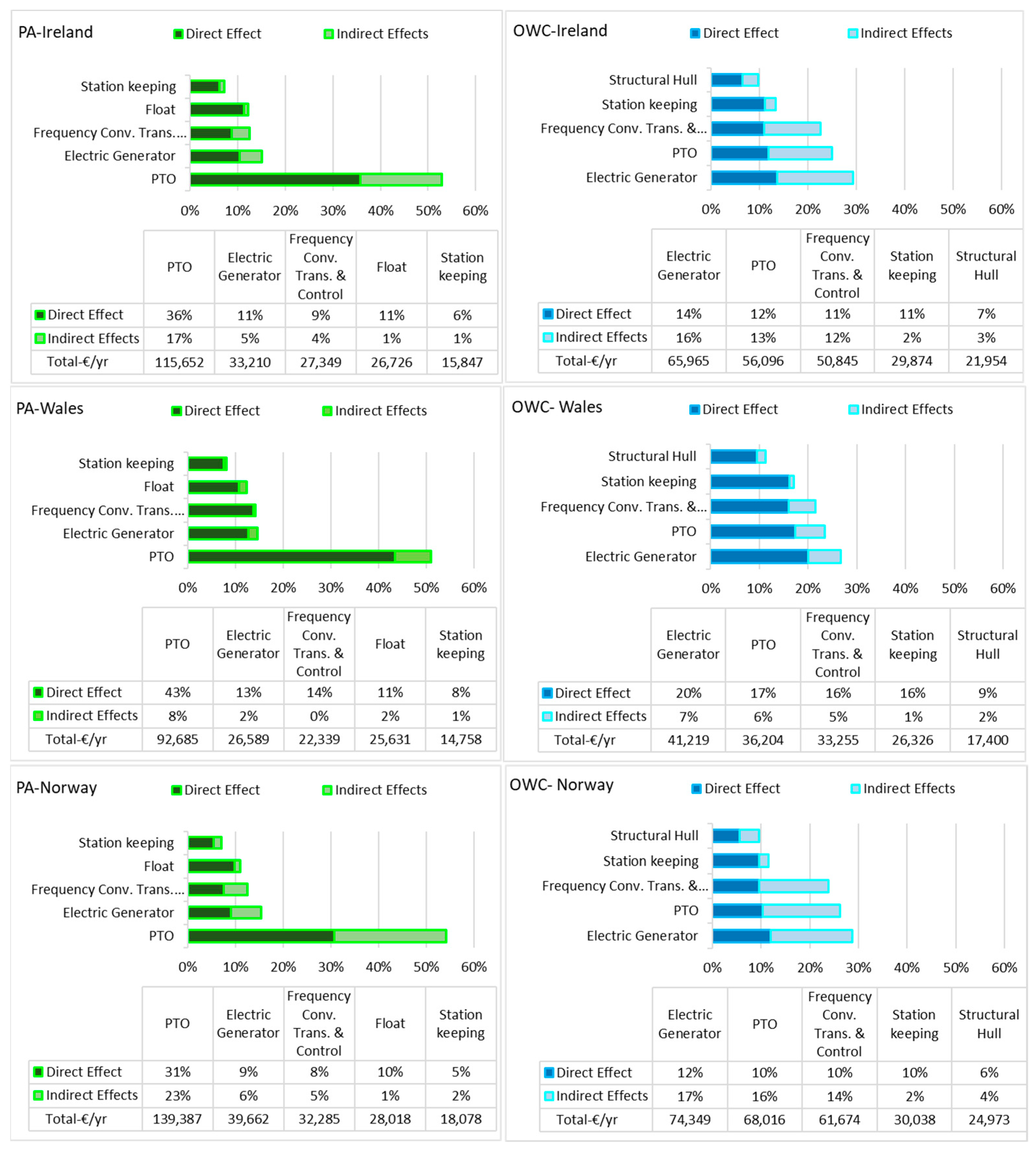
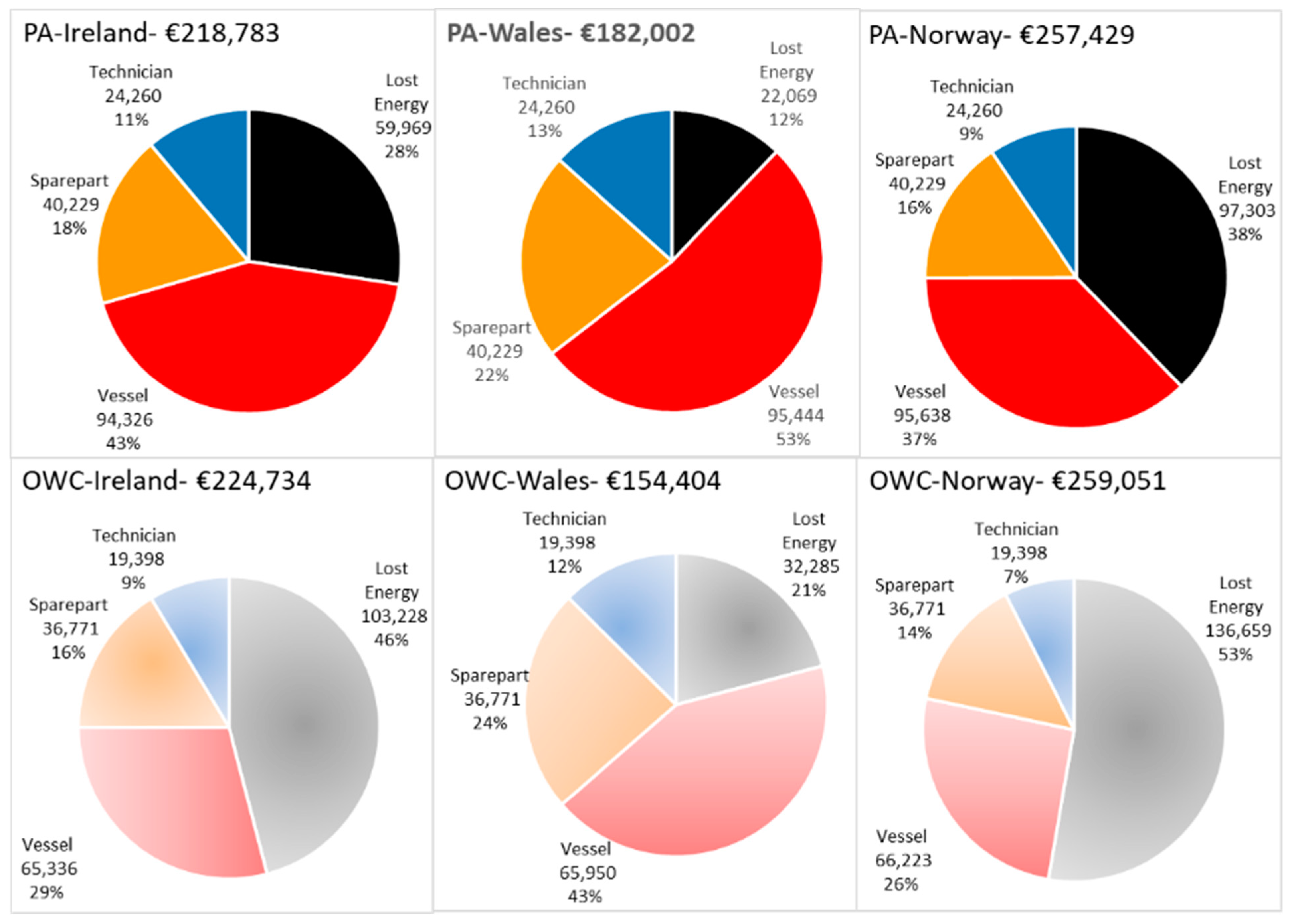
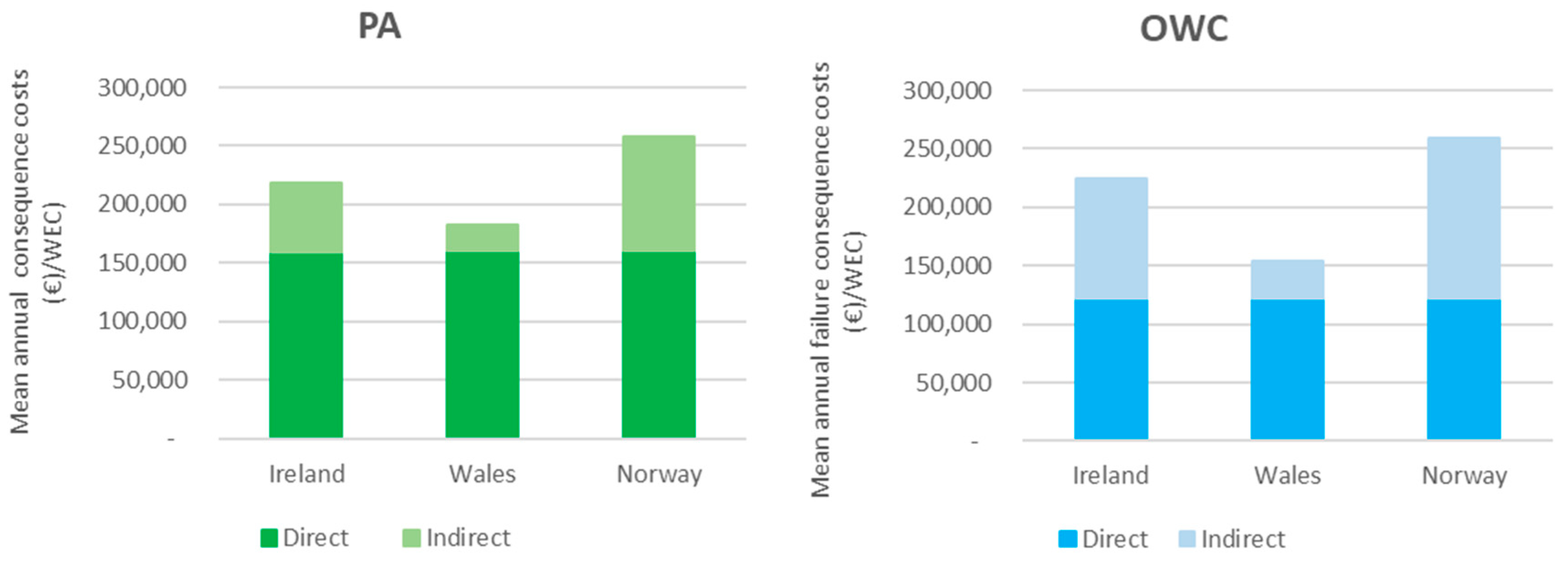
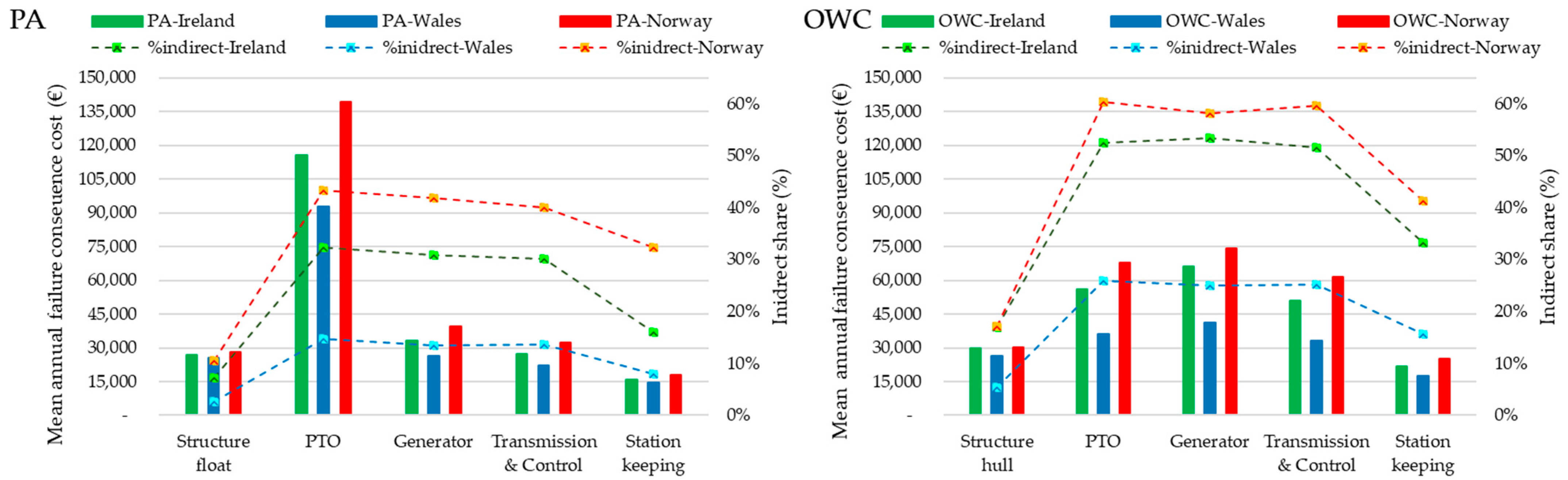
3.1. Failure Consequence Costs
- (1)
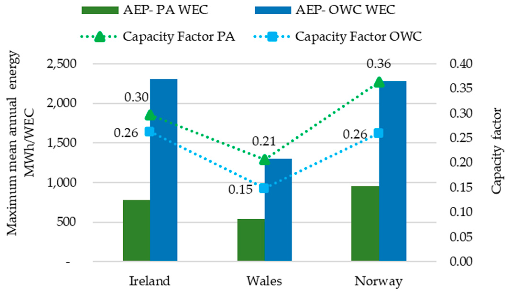
- The AEP of each device, which is related to the device capacity factor (CF), is the ratio of the average power generated, e.g., over the course of a year, by a fully functional WEC to the maximum rated power that can be generated [63]. Figure 5 compares the AEP and CF of the two WECs. The AEP and CF of PA in Norway are higher by 22% and 76% compared to PA in Ireland and PA in Wales, respectively. For OWC, these metrics in Wales are 43% lower than those in Norway, but they are nearly identical in Norway and Ireland.
- (2)
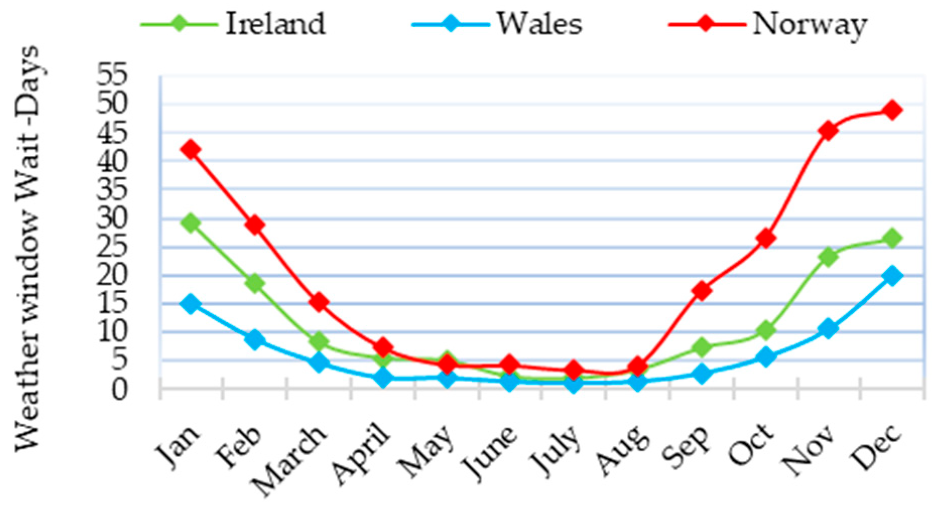
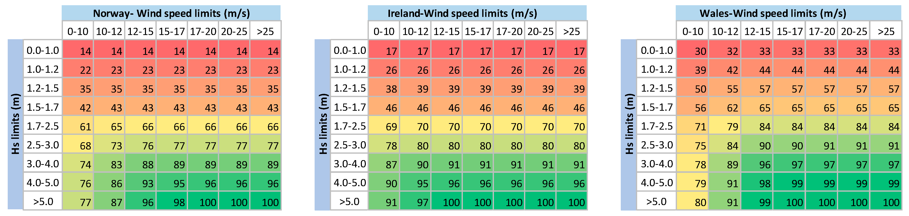
- The mean weather window waiting time of sites (an important element affecting the downtime and actual MTTR). Figure 6 compares the weather window waiting times of the three sites.
- (3)
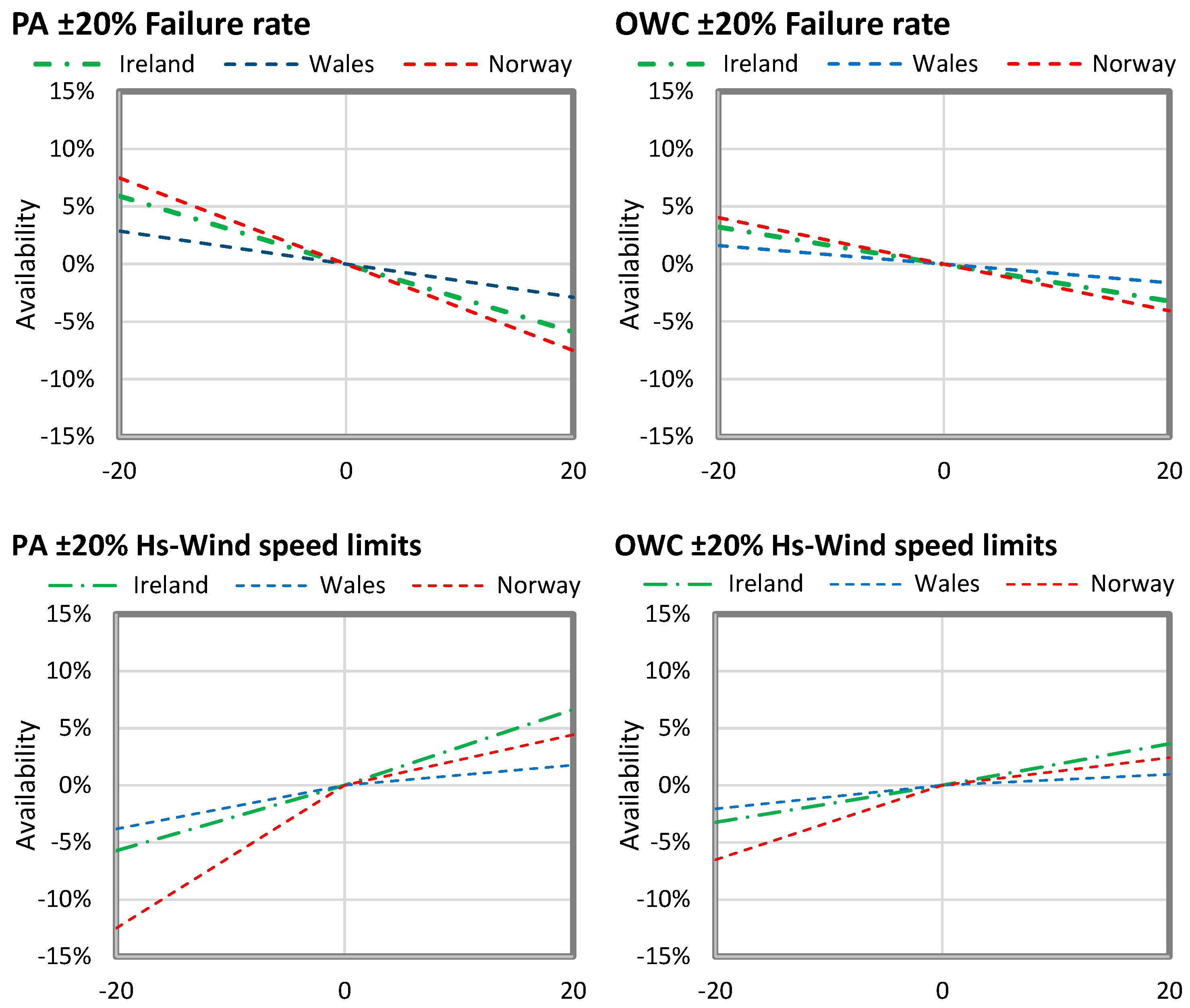
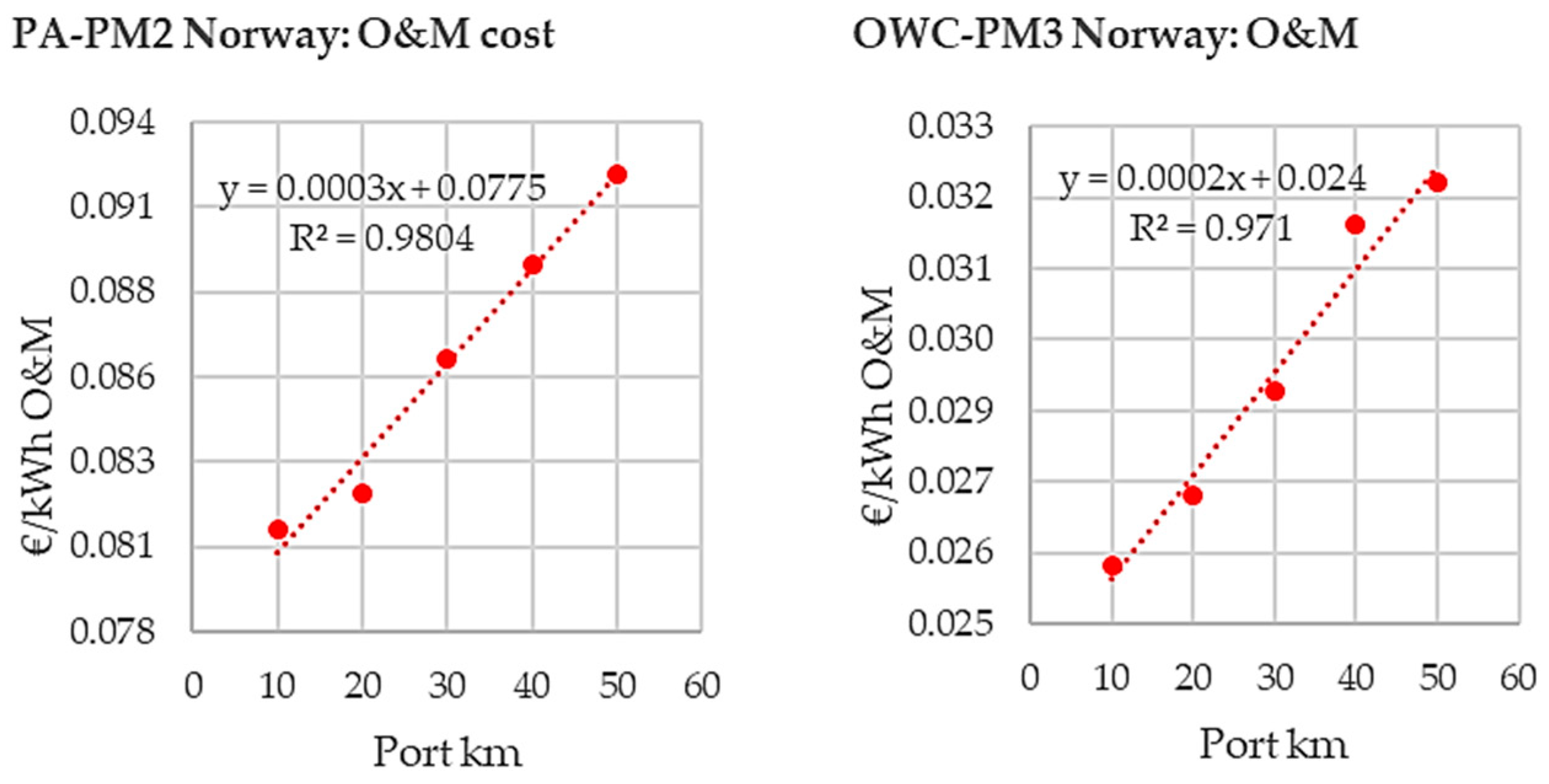
Sensitivity Analysis
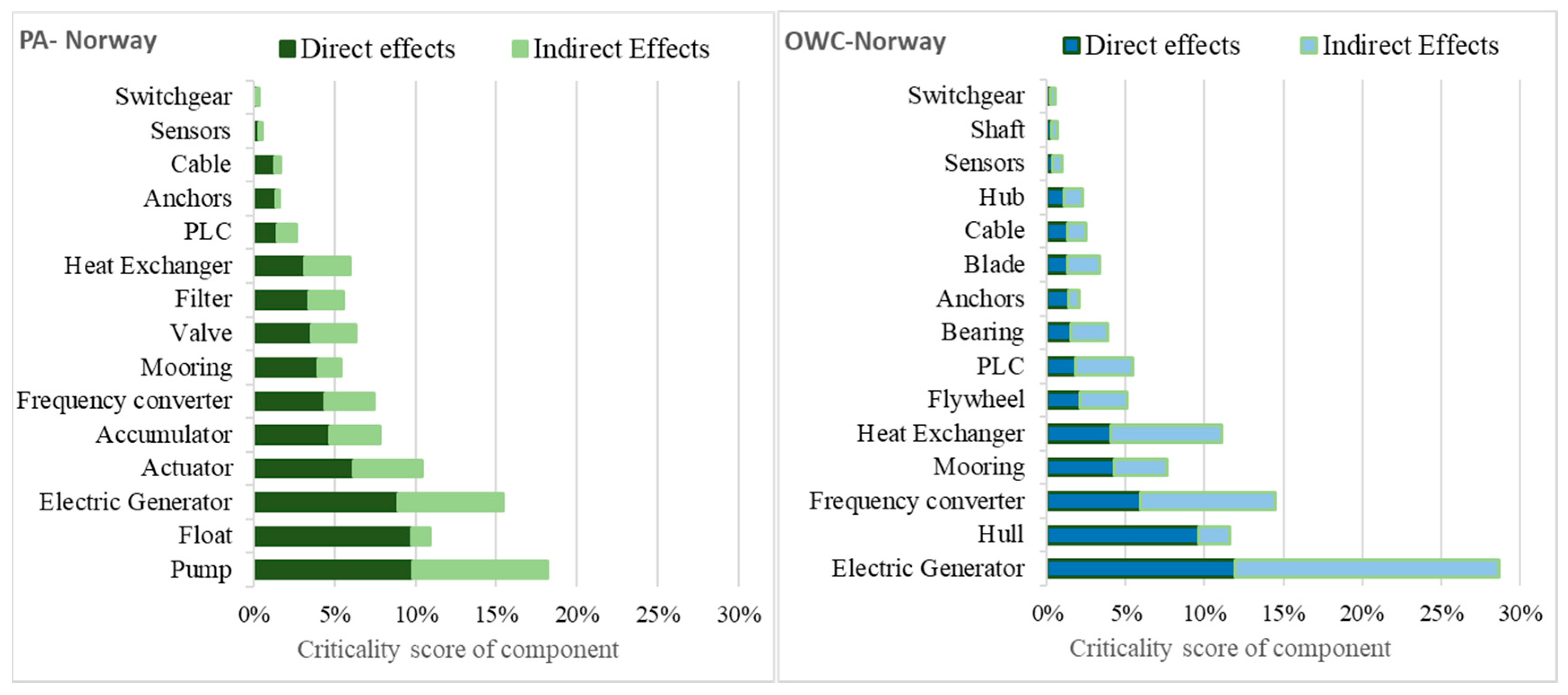
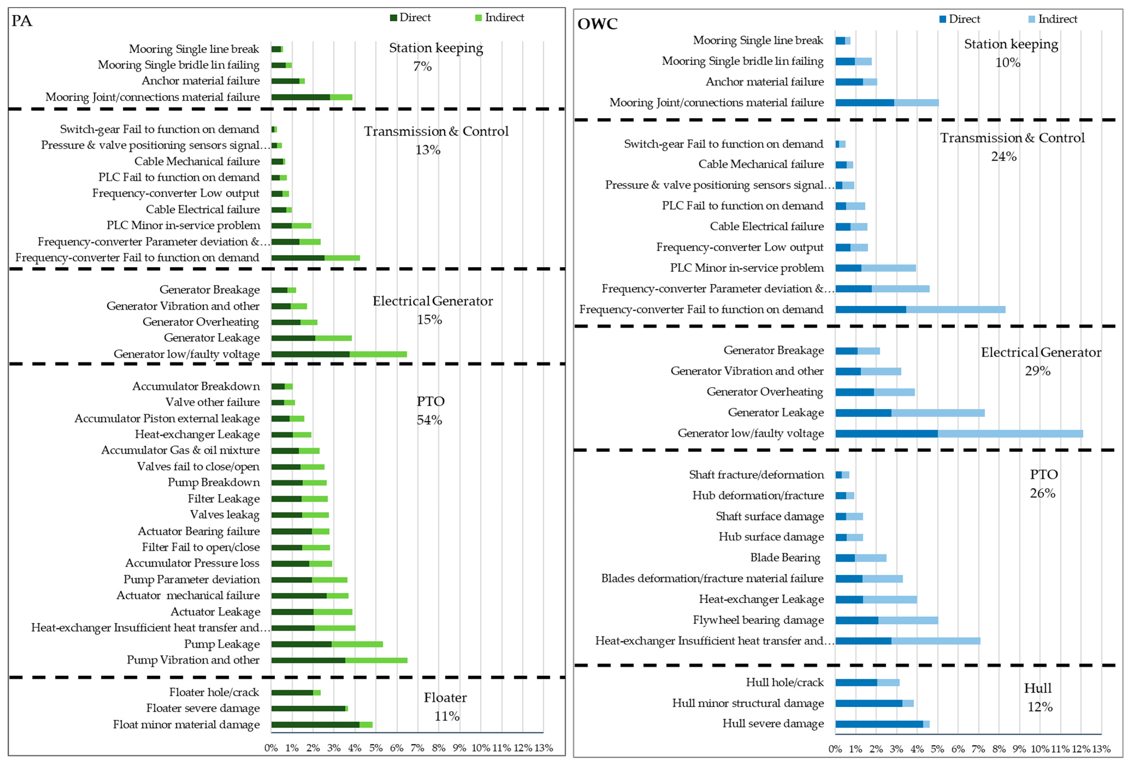
3.2. Failure Mode Consequence Cost Ranking
PM Scenario Analysis
- Which subsystem and which failure mode within a subsystem/component has a bigger effect on the failure consequence costs for a specific location or type of WEC, both in terms of direct repair costs and indirect costs? (See Section 3.1 and Section 3.2). These quantitative measures can be used, much in line with an FMECA approach, to help guide decisions about enhancing product reliabilities at various stages of development.
- How does the case study location impact the assessed metrics for a particular WEC type? Or which type of WEC is preferred in a particular location given the inputs and their sensitivity in the case study? (See Section 3.1).
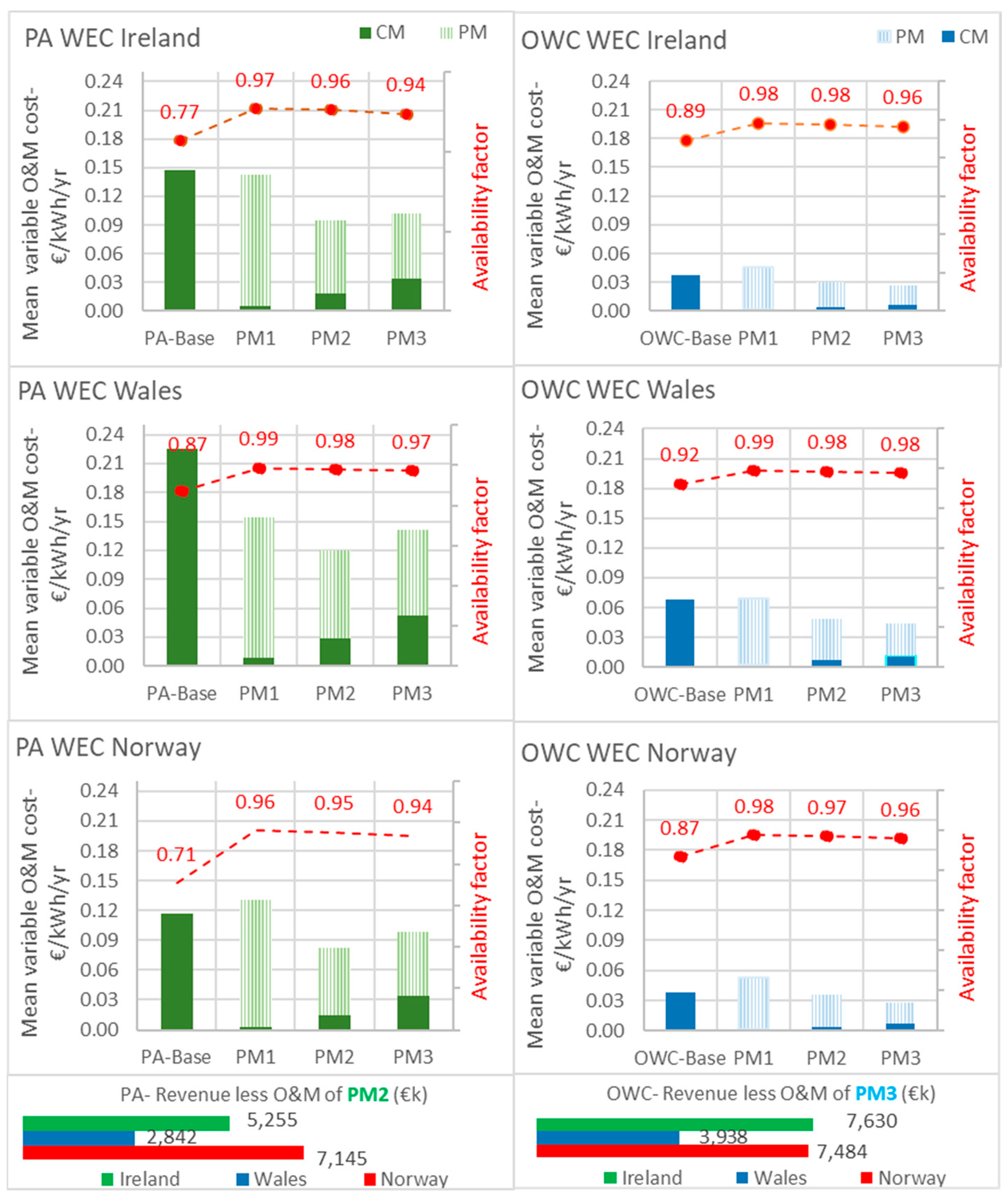
- If PM is used as a potential failure-mitigation option, which PM interval is ideal in terms of reducing O&M costs, gaining an acceptable availability, and increasing operating profits? What percentage of projected WEC farms’ O&M expenses are related to CM and PM? (See Section PM Scenario Analysis).
4. Remarks and Future Studies
5. Conclusions
Author Contributions
Funding
Data Availability Statement
Acknowledgments
Conflicts of Interest
Appendix A
References
- Heikkilä, E.; Välisalo, T.; Tiusanen, R.; Sarsama, J.; Räikkönen, M. Reliability Modelling and Analysis of the Power Take-Off System of an Oscillating Wave Surge Converter. J. Mar. Sci. Eng. 2021, 9, 552. [Google Scholar] [CrossRef]
- Galparsoro, I.; Liria, P.; Legorburu, I.; Bald, J.; Chust, G.; Ruiz-Minguela, P.; Pérez, G.; Marqués, J.; Torre-Enciso, Y.; González, M.; et al. A Marine Spatial Planning Approach to Select Suitable Areas for Installing Wave Energy Converters (WECs), on the Basque Continental Shelf (Bay of Biscay). Coast. Manag. 2012, 40, 1–19. [Google Scholar] [CrossRef]
- European Union. An EU Strategy to Harness the Potential of Offshore Renewable Energy for a Climate Neutral Future; EU: Brussels, Belgium, 2020; p. 27. [Google Scholar]
- OEE. Ocean Energy Europe. Key Trands and Statistics 2021. Ocean Energy. 2022. Available online: https://www.oceanenergy-europe.eu/wp-content/uploads/2022/03/OEE_Stats_and_Trends_2021_web.pdf (accessed on 10 February 2024).
- Jones, C.; Chang, G.; Dallman, A.; Roberts, J.; Raghukumar, K.; McWilliams, S. Assessment of wave energy resources and factors affecting conversion. In Proceedings of the Offshore Technology Conference, Houston, TX, USA, 6–9 May 2019. [Google Scholar] [CrossRef]
- PRIMRE. Portal and Repository for Information on Marine Renewable Energy—PRIMRE Databases. 2023. Available online: https://openei.org/wiki/PRIMRE/Databases/Projects_Database (accessed on 10 December 2023).
- IRENA. Innovation Outlook: Ocean Energy Technologies; IRENA: Masdar City, United Arab Emirates, 2020. [Google Scholar]
- Magagna, D.; Uihlein, A. Ocean energy development in Europe: Current status and future perspectives. Int. J. Mar. Energy 2015, 11, 84–104. [Google Scholar] [CrossRef]
- OES—IEA. International Levelised Cost of Energy for Ocean Energy Technologies. 2015. Available online: https://www.ocean-energy-systems.org/oes-projects/levelised-cost-of-energy-assessment-for-wave-tidal-and-otec-at-an-international-level/ (accessed on 10 December 2023).
- October, R.; Working, I.; Ocean, G. SET-Plan Ocean Energy—Implementation Plan. vol. 2021, no. March 2018, 2021. Available online: https://setis.ec.europa.eu/document/download/8d2ad133-13ee-441f-9776-46c7aef98714_en?filename=SET%20Plan%20OCEAN%20ENERGY%20Implementation%20plan.pdf (accessed on 19 July 2024).
- Göteman, M.; Shahroozi, Z.; Stavropoulou, C.; Katsidoniotaki, E.; Engström, J. Resilience of wave energy farms using metocean dependent failure rates and repair operations. Ocean Eng. 2023, 280, 114678. [Google Scholar] [CrossRef]
- Guo, C.; Sheng, W.; De Silva, D.G.; Aggidis, G. A Review of the Levelized Cost of Wave Energy Based on a Techno-Economic Model. Energies 2023, 16, 2144. [Google Scholar] [CrossRef]
- Castro-Santos, L.; Filgueira-Vizoso, A.; Costoya, X.; Arguilé-Pérez, B.; Ribeiro, A.S. Economic viability of floating wave power farms considering the energy generated in the near future. Renew. Energy 2024, 222, 119947. [Google Scholar] [CrossRef]
- O’Connell, R.; Kamidelivand, M.; Furlong, R.; Guerrini, M.; Cullinane, M.; Murphy, J. An advanced geospatial assessment of the Levelised cost of energy (LCOE) for wave farms in Irish and western UK waters. Renew. Energy 2024, 221, 119864. [Google Scholar] [CrossRef]
- Chang, G.; Jones, C.A.; Roberts, J.D.; Neary, V.S. A comprehensive evaluation of factors affecting the levelized cost of wave energy conversion projects. Renew. Energy 2018, 127, 344–354. [Google Scholar] [CrossRef]
- OpenEI. Open Energy Information, Data and Resources Primre/Tools. Available online: https://openei.org/wiki/PRIMRE/Tools (accessed on 15 April 2024).
- Aalborg University. An Open-Access COE Calculation Tool for Wave Energy Converters: The Danish Approach. Available online: https://vbn.aau.dk/en/publications/an-open-access-coe-calculation-tool-for-wave-energy-converters-th (accessed on 15 March 2024).
- NREL. WEC-Sim Wave Energy Converter Simulator. Available online: https://data.nrel.gov/submissions/39 (accessed on 15 February 2024).
- Sandia National Laboratories. Optimal Design Tools for Ocean Energy Arrays (DTOcean). Available online: https://energy.sandia.gov/programs/renewable-energy/water-power/projects/dtocean/ (accessed on 20 May 2024).
- SELKIE Tools. Logistics and Operation and Maintenance (O&M) Decision-Support Tool. Available online: https://www.selkie-project.eu/logistics-and-operation-and-maintenance-om-decision-support-tool/ (accessed on 10 June 2024).
- Rodrigues, J.M.; Langhele, N.K.; Rølvåg, T.; Cruz, J.; Cruz, M.A.; Martini, M.; Garcia-Rosa, P.B.; Kamidelivand, M.; Alessandri, G.; Gallorini, F. Compilation of Development Metrics Applicable to Wave Energy Converters (WECs): Current Status and Proposed Next Steps. In Proceedings of the 33rd International Ocean and Polar Engineering Conference, Ottawa, SO, Canada, 19–23 June 2023. [Google Scholar] [CrossRef]
- Hodges, J.; Henderson, J.; Ruedy, L.; Soede, M.; Weber, J.; Ruiz-Minguela, P.; Jeffrey, H.; Bannon, E.; Holland, M.; Maciver, R.; et al. An International Evaluation and Guidance Framework for Ocean Energy Technology 2O21 2-Task 12. 2021. Available online: www.formasdopossivel.com (accessed on 10 May 2024).
- MIL-STD-1629. Failure Mode Effects and Criticality Analysis. 1993. Available online: https://www.sciencedirect.com/science/article/abs/pii/0026271472903927?via%3Dihub (accessed on 8 December 2023).
- Scheu, M.N.; Tremps, L.; Smolka, U.; Kolios, A.; Brennan, F. A systematic Failure Mode Effects and Criticality Analysis for offshore wind turbine systems towards integrated condition based maintenance strategies. Ocean Eng. 2019, 176, 118–133. [Google Scholar] [CrossRef]
- Cevasco, D.; Collu, M.; Lin, Z. O&M Cost-Based FMECA: Identification and Ranking of the Most Critical Components for 2–4 MW Geared Offshore Wind Turbines. In Proceedings of the WindEurope Conference 2018 within the Global Wind, Hamburg, Germany, 25–28 September 2018; Volume 1102. [Google Scholar] [CrossRef]
- Tazi, N.; Châtelet, E.; Bouzidi, Y. Using a hybrid cost-FMEA analysis for wind turbine reliability analysis. Energies 2017, 10, 276. [Google Scholar] [CrossRef]
- Rinaldi, G.; Thies, P.R.; Walker, R.; Johanning, L. On the Analysis of a Wave Energy Farm with Focus on Maintenance Operations. J. Mar. Sci. Eng. 2016, 4, 51. [Google Scholar] [CrossRef]
- Gray, A.; Dickens, B.; Bruce, T.; Ashton, I.; Johanning, L. Reliability and O&M sensitivity analysis as a consequence of site specific characteristics for wave energy converters. Ocean Eng. 2017, 141, 493–511. [Google Scholar] [CrossRef]
- CarbonTrust. Guidelines on Design and Operation of Wave Energy Converters: A Guide to Assessment and Application of Engineering Standards and Recommended Practices for Wave Energy Conversion Devices; CarbonTrust: London, UK, 2005. [Google Scholar]
- Bertram, D.V.; Tarighaleslami, A.H.; Walmsley, M.R.W.; Atkins, M.J.; Glasgow, G.D.E. A systematic approach for selecting suitable wave energy converters for potential wave energy farm sites. Renew. Sustain. Energy Rev. 2020, 132, 110011. [Google Scholar] [CrossRef]
- Neary, V.S.; Lawson, M.; Previsic, M.; Copping, A.; Hallett, K.C.; Labonte, A.; Rieks, J.; Murray, D. Methodology for Design and Economic Analysis of Marine Energy Conversion (MEC) Technologies; Sandia National Laboratories: Livermore, CA, USA, 2014; p. 261. [Google Scholar]
- Bull, D.L.; Smith, C.; Jenne, D.S.; Jacob, P.; Copping, A.; Willits, S.; Fontaine, A.; Brefort, D.; Gordon, M.E.; Copeland, R.; et al. Reference Model 6 (RM6): Oscillating Wave Energy Converter; Sandia National Laboratories: Livermore, CA, USA, 2014; Volume 6. [Google Scholar]
- Raj, N.; Bharathi, K. Electrical Networks of CorPower Wave Farms: Economic Assessment and Grid Integration Analysis. 2017. Available online: https://www.semanticscholar.org/paper/Electrical-Networks-of-CorPower-Wave-Farms-%3A-and-of-Bharathi/69f2210536eafcd242384b6d5c40d8a0f08c2e05 (accessed on 8 April 2024).
- Kamidelivand, M.; Deeney, P.; McAuliffe, F.D.; O’Connell, R.; Mulcahy, I.; Murphy, J. Adapting Optimal Preventive Maintenance Strategies for Floating Offshore Wind in Atlantic Areas by Integrating O&M Modelling and FMECA. In Proceedings of the OCEANS 2023—Limerick, Limerick, Ireland, 5–8 June 2023; pp. 1–8. [Google Scholar] [CrossRef]
- Judge, F.; McAuliffe, F.D.; Sperstad, I.B.; Chester, R.; Flannery, B.; Lynch, K.; Murphy, J. A lifecycle financial analysis model for offshore wind farms. Renew. Sustain. Energy Rev. 2019, 103, 370–383. [Google Scholar] [CrossRef]
- Chen, J. Uniform Distribution: Definition, How It Works and Example. Investopedia, 2023. Distributions Are Probability Distributions, the Mean Occur More Frequently. Available online: https://www.investopedia.com/terms/u/uniform-distribution.asp#:~:text=Uniform (accessed on 8 May 2024).
- Kamidelivand, M.; Deeney, P.; McAuliffe, F.D.; Leyne, K.; Togneri, M.; Murphy, J. Scenario Analysis of Cost-Effectiveness of Maintenance Strategies for Fixed Tidal Stream Turbines in the Atlantic Ocean. J. Mar. Sci. Eng. 2023, 11, 1046. [Google Scholar] [CrossRef]
- McAuliffe, F.D.; Judge, F.; Kamidelivand, M. Modified Installation, Operations, Maintenance and Logistics Model for Irish and Welsh Wave and Tidal Technologies and Locations. 2022. Available online: https://www.selkie-project.eu/tools/wp8/ (accessed on 10 May 2024).
- Lotovskyi, E.; Teixeira, A.P.; Soares, C.G. Availability analysis of an offshore oil and gas production system subjected to age-based preventive maintenance by petri nets. Eksploat. Niezawodn. 2020, 22, 627–637. [Google Scholar] [CrossRef]
- Nguyen, T.A.T.; Chou, S.Y. Improved maintenance optimization of offshore wind systems considering effects of government subsidies, lost production and discounted cost model. Energy 2019, 187, 115909. [Google Scholar] [CrossRef]
- The WAVEWATCH Development Group. WW3DG. User Manual and System Documentation of WAVEWATCH III Version 6.07; NOAA/NWS/NCEP/MMAB Technical Note 2019; p. 311. Available online: https://polar.ncep.noaa.gov/waves/wavewatch/manual.v5.16.pdf (accessed on 19 July 2024).
- Chawla, A.; Spindler, D.M.; Tolman, H.L. Validation of a thirty year wave hindcast using the Climate Forecast System Reanalysis winds. Ocean Model. 2013, 70, 189–206. [Google Scholar] [CrossRef]
- Copernicus. ERA5 Hourly Data on Single Levels from 1959 to Present (2022). Available online: https://cds.climate.copernicus.eu/%0Acdsapp#!/dataset/reanalysis-era5-single-levels?tab=overview (accessed on 1 December 2022).
- O’Connell, R.; Furlong, R.; Guerrini, M.; Cullinane, M.; Murphy, J. Development and Application of a GIS for Identifying Areas for Ocean Energy Deployment in Irish and Western UK Waters. J. Mar. Sci. Eng. 2023, 11, 826. [Google Scholar] [CrossRef]
- Rusu, L.; Rusu, E. Evaluation of the worldwide wave energy distribution based on ERA5 data and altimeter measurements. Energies 2021, 14, 394. [Google Scholar] [CrossRef]
- Neary, V.S.; Coe, R.G.; Cruz, J.; Haas, K.; Bacelli, G.; Debruyne, Y.; Ahn, S.; Nevarez, V. Classification systems for wave energy resources and WEC technologies. Int. Mar. Energy J. 2018, 1, 71–79. [Google Scholar] [CrossRef]
- Rosati, M.; Henriques, J.C.C.; Ringwood, J.V. Oscillating-water-column wave energy converters: A critical review of numerical modelling and control. Energy Convers. Manag. X 2022, 16, 100322. [Google Scholar] [CrossRef]
- Blain, L. Giant, Megawatt-Scale Wave Energy Generator to be Tested in Scotland. NEW ATLAS, 2022. Available online: https://newatlas.com/energy/oceanenergy-oe35-wave-power/ (accessed on 7 May 2024).
- Nambiar, A.J.; Collin, A.J.; Karatzounis, S.; Rea, J.; Whitby, B.; Jeffrey, H.; Kiprakis, A.E. Optimising power transmission options for marine energy converter farms. Int. J. Mar. Energy 2016, 15, 127–139. [Google Scholar] [CrossRef]
- Hamedni, B.; Cocho, M.; Ferreira, C.B. Generic WEC System Breakdown; Deliverable 5.1. The Structural Design of Wave Energy Devices (SDWED) Project; DNV.GL: Bærum, Norway, 2014; pp. 1–41. [Google Scholar]
- Pecher, A.; Kofoed, J.P. Handbook of Ocean Wave Energy. Ocean Engineering & Oceanography Volume 7; Springer International Publishing: Berlin/Heidelberg, Germany, 2017. [Google Scholar]
- Mérigaud, A.; Ringwood, J.V. Power production assessment for wave energy converters: Overcoming the perils of the power matrix. J. Eng. Marit. Environ. 2018, 232, 50–70. [Google Scholar] [CrossRef]
- Bozzi, S.; Besio, G.; Passoni, G. Wave power technologies for the Mediterranean offshore: Scaling and performance analysis. Coast. Eng. 2018, 136, 130–146. [Google Scholar] [CrossRef]
- Xu, X.; Robertson, B.; Buckham, B. A techno-economic approach to wave energy resource assessment and development site identification. Appl. Energy 2020, 260, 114317. [Google Scholar] [CrossRef]
- Anderson, F.; Dawid, R.; Cava, D.G.; McMillan, D. Operational Metrics for an Offshore Wind Farm & Their Relation to Turbine Access Restrictions and Position in the Array. In Proceedings of the EERA DeepWind’2021, Trondheim, Norway, 13–15 January 2021. [Google Scholar] [CrossRef]
- Kamidelivand, M.; Murphy, J. FMECA DataBase H2020 IMPACT D4.1. 2022. Available online: https://zenodo.org/records/7839861 (accessed on 10 May 2024).
- Hamedni, B.; Ferreia, C.B. Generic WEC Risk Ranking and Failure Mode Analysis; The Structural Design of Wave Energy Device (SDWED) project. Deliverable D5.2; DNV GL: Bærum, Norway, 2014. [Google Scholar]
- Rhinefrank, K. StingRAY Failure Mode, Effects and Criticality Analysis: WEC Risk Registers [Data Set]. 2016. Available online: https://www.osti.gov/biblio/1415597 (accessed on 5 January 2024).
- Mueller, M.; Lopez, R.; McDonald, A.; Jimmy, G. Reliability analysis of wave energy converters. In Proceedings of the 2016 IEEE International Conference on Renewable Energy Research and Applications (ICRERA), Birmingham, UK, 20–23 November 2016; Volume 5, pp. 667–672. [Google Scholar] [CrossRef]
- Gueguen, S.; Fourmigué, J.-M. Risk Assessment of Marine Energy Projects; KTH School of Industrial Engineering and Management: Stockholm, Sweden, 2016. [Google Scholar]
- Lopez-Mendia, J.; Ruiz-Minguela, P.; Rodríguez, R.; De Miguel Etxaniz, P.; Flannery, B.; Goodwin, P. Deliverable D6.2, OPERA—Operational Model for Offshore Operation of Wave Energy Converters—Open Sea Operating Experience to Reduce Wave Energy Costs. Available online: https://proactive-h2020.eu/wp-content/uploads/2021/04/PROACTIVE_20210312_D6.2_V5_PHE_Scenario-Development-and-Evaluation-Methodology_revised.pdf (accessed on 14 June 2024).
- Ahn, D.; Shin, S.C.; Kim, S.Y.; Kharoufi, H.; Kim, H.C. Comparative evaluation of different offshore wind turbine installation vessels for Korean west–south wind farm. Int. J. Nav. Archit. Ocean Eng. 2017, 9, 45–54. [Google Scholar] [CrossRef]
- Starling, M. Guidelines for Reliability, Maintainability and Survivability of Marine Energy Conversion Systems. Marine Renewable Energy Guides; European Marine Energy Centre: Stromness, Scotland, 2009. [Google Scholar]
- Jusoh, M.A.; Ibrahim, M.Z.; Daud, M.Z.; Albani, A.; Yusop, Z.M. Hydraulic power take-off concepts for wave energy conversion system: A review. Energies 2019, 12, 4510. [Google Scholar] [CrossRef]
- Coe, R.G.; Ahn, S.; Neary, V.S.; Kobos, P.H.; Bacelli, G. Maybe less is more: Considering capacity factor, saturation, variability, and filtering effects of wave energy devices. Appl. Energy 2021, 291, 116763. [Google Scholar] [CrossRef]
- DNVGL-RP-203. Fatigue Design of Offshore Steel Structures- Recommended Practice. 2021. Available online: https://www.dnv.com/oilgas/download/dnv-rp-c203-fatigue-design-of-offshore-steel-structures.html (accessed on 5 April 2024).
- Mortazavizadeh, S.A.; Yazdanpanah, R.; Gaona, D.C.; Anaya-Lara, O. Fault Diagnosis and Condition Monitoring in Wave Energy Converters: A Review. Energies 2023, 16, 6777. [Google Scholar] [CrossRef]
- ROMEO-D2.1. Failure Mode Diagnosis/Prognosis Orientations. No. 745625, 2020. Available online: https://www.romeoproject.eu/wp-content/uploads/2019/06/D2.1_ROMEO_Failure_mode_diagnosis_prognosis_orientations.pdf (accessed on 8 February 2024).
- Marie-Antoinette, S.; Borisade, F.; Espelage, J.; Johnson, E.; Vicente, R.D.; Munoz, S.; Hylland, P.; He, W.; Urbano, J.; Comas, F.J.; et al. COREWIND D4.2 Floating Wind O&M Strategies Assessment. no. August, 2021. Available online: http://corewind.eu/wp-content/uploads/files/publications/COREWIND-D4.2-Floating-Wind-O-and-M-Strategies-Assessment.pdf (accessed on 19 July 2024).
- Aderinto, T.; Li, H. Review on Power Performance and Efficiency of Wave Energy Converters. Energies 2019, 12, 4329. [Google Scholar] [CrossRef]


| Site | Parameter | Spatial Resolution | Temporal Resolution and Period | Data and Model | Reference |
|---|---|---|---|---|---|
| West Ireland and Wales | Wave data (Hs and Tp) | 0.017° × 0.017° | Three-hourly * 2000–2019 | Copernicus Atlantic—European North-West Shelf-Wave Phsics Reanlayis; underlying model: Wave watchIII | [44] |
| Wind | 0.25° × 0.25° | Hourly 1940–2022 | Copernicus ERA5 hourly data on single levels; underlying model: the European centre for Medium-Range Weather Forcecasts (ECMWF) | ||
| Norway | Wave and Wind data | 0.25° × 0.25° | Three-hourly * 1979–2009 | WaveWatch III third-generation wave model, developed at the US National Centers for Environmental Prediction (NOAA/NCEP) in line with the WAM model | [41,42] |
| Parameter | Ireland | Wales | Norway |
|---|---|---|---|
| Wind speed (m/s) | |||
| Mean | 6.7 | 7.8 | 8.3 |
| 25 percentile | 4.4 | 5.1 | 4.8 |
| 75 percentile | 8.6 | 10.3 | 11.1 |
| Tp (s) | |||
| Mean | 10.9 | 9.6 | 9.5 |
| 25 percentile | 9.1 | 7.5 | 7.4 |
| 75 percentile | 12.4 | 11.6 | 11.1 |
| Hs (m) | |||
| Mean | 2.3 | 1.8 | 2.5 |
| 25 percentile | 1.2 | 0.9 | 1.4 |
| 75 percentile | 3.0 | 2.3 | 3.2 |
| Wave energy intensity (kW/m) * | |||
| Mean | 40.2 | 19.3 | 39.0 |
| 25 percentile | 6.6 | 3.0 | 6.7 |
| 75 percentile | 45.2 | 21.4 | 45.7 |
| Subsystem | Component | Most Common Failure Types | Annual Failure Rate | Most Common Failure Causes | Material Cost (EUR) |
|---|---|---|---|---|---|
| Structure | Float a Hull b | Minor material damage | 0.300 | Marine growth, weather impact, other Severe storm, lightning, corrosion, fatigue, collision | 10,000 |
| 0.180 b | 15,000 b | ||||
| Major structural damage | 0.010 | 800,000 1,000,000 b | |||
| Hole/Crack | 0.032 | 80,000 | |||
| PTO | Actuators a | Leakage | 0.196 | Seal failure, rod corrosion, high pressure | 1500 |
| Mechanical failure | 0.110 | 30,000 | |||
| Bearing failure | 0.080 | 30,000 | |||
| Accumulator a | Piston external leakage | 0.084 | Contamination, corrosion, jammed piston | 1500 | |
| Pressure loss | 0.117 | 15,000 | |||
| Gas and oil mixture | 0.101 | 2000 | |||
| Breakdown | 0.035 | 15,000 | |||
| Pump (motor) a | Parameter deviation | 0.188 | Clearance/alignment, mechanical failure, overheating, wear | 1500 | |
| Leakage | 0.273 | 1500 | |||
| Breakdown | 0.117 | 6500 | |||
| Vibration and other | 0.275 | 6500 | |||
| Valve (general) a | Leakage | 0.143 | Clearance/alignment, contamination, deformation, looseness | 2500 | |
| Fail to close/open | 0.139 | 2500 | |||
| Other failure | 0.060 | 2500 | |||
| Filter (general) a | Leakage | 0.143 | Plug, material failure, looseness | 2500 | |
| Fail to open/close | 0.143 | 2500 | |||
| Heat exchanger (generic) | Leakage | 0.099 | Blockage, corrosion, wear, mechanical failure | 1500 | |
| Insufficient heat transfer | 0.205 | 5000 | |||
| Air wells turbine b | Hub deformation/fracture | 0.015 | Wear, vibration, corrosion, contamination ingress, lubrication fail | 50,000 | |
| Hub surface damage | 0.035 | 8000 | |||
| Blades deformation/fracture | 0.069 | 15,000 | |||
| Bearing | 0.050 | 10,000 | |||
| Surface damage | 0.035 | 5000 | |||
| Shaft deformation/fracture Flywheel bearing damage | 0.012 0.123 | 25,000 10,000 |
| Subsystem | Component | Most Common Failure Mode | Annual Failure Rate | Most Common Failure Cause | Spare-Part Cost (EUR) * |
|---|---|---|---|---|---|
| Electric generator | Electric generator | Leakage | 0.202 | Blockage, cavitation, corrosion, mechanical failure, short circuit, software failure, vibration | 2000 |
| Breakage | 0.043 | 15,000 | |||
| Overheating | 0.078 | 15,000 | |||
| Low/faulty output voltage | 0.324 | 5000 | |||
| Vibration and other | 0.081 | 5000 | |||
| Transmission and Control | Transformer converter | Fail to function on demand | 0.182 | Mechanical failure, leakage, open circuit, short circuit, general electrical failure, software failure | 10,000 |
| Low output | 0.034 | 15,000 | |||
| Parameter deviation and other | 0.114 | 5000 | |||
| Switch gear | Fail to function on demand | 0.010 | Breakage, general electrical failure, software | 2000 | |
| Cable | Mechanical failure | 0.010 | Damage to tension members of the cable, corrosion, wear, and damage to insultation | 90,000 | |
| Electrical failure | 0.030 | 10,000 | |||
| Sensor Programmable Logic Controller (PLC) | Signal failure | 0.030 | Blockage and control failure clearance, faulty alarm, general instrument failure, and software | 1000 | |
| Fail to function on demand | 0.037 | 4000 | |||
| Minor in-service problem | 0.099 | 1000 |
| Subsystem | Component | Most Common Failure Mode | Annual Failure Rate | Most Common Failure Cause | Spare-Part Cost (EUR) |
|---|---|---|---|---|---|
| Station-keeping | Mooring lines | Single bridle line failing | 0.030 | Material degradation, Environmental issues, corrosion | 10,000 |
| Single line break | 0.010 | 60,000 * | |||
| Joint/connection | Material failure | 0.110 | Fatigue, corrosion, and marine growth | 15,000 | |
| Anchor | Material failure | 0.030 | 65,000 * |
| Vessel Types | ||
|---|---|---|
| Parameter | Tug-Boat Pair | Multipurpose Workboat |
| Max Wave, m | 1.2 | 1.75 |
| Max Wind, m/s | 15 | 20 |
| Daily hire, EUR | 6000 (10,000) * | 20,000 |
| Mobilisation fee, EUR | 8000 (12,000) * | 25,000 |
| Mobilisation time, hr | 72 | 168 |
| Mean speed, knot ** | 12 | 17 |
| Mean fuel L/h | 150 (250) * | 300 |
Disclaimer/Publisher’s Note: The statements, opinions and data contained in all publications are solely those of the individual author(s) and contributor(s) and not of MDPI and/or the editor(s). MDPI and/or the editor(s) disclaim responsibility for any injury to people or property resulting from any ideas, methods, instructions or products referred to in the content. |
© 2024 by the authors. Licensee MDPI, Basel, Switzerland. This article is an open access article distributed under the terms and conditions of the Creative Commons Attribution (CC BY) license (https://creativecommons.org/licenses/by/4.0/).
Share and Cite
Kamidelivand, M.; Deeney, P.; Murphy, J.; Rodrigues, J.M.; Garcia-Rosa, P.B.; Atcheson Cruz, M.; Alessandri, G.; Gallorini, F. Failure Consequence Cost Analysis of Wave Energy Converters—Component Failures, Site Impacts, and Maintenance Interval Scenarios. J. Mar. Sci. Eng. 2024, 12, 1251. https://doi.org/10.3390/jmse12081251
Kamidelivand M, Deeney P, Murphy J, Rodrigues JM, Garcia-Rosa PB, Atcheson Cruz M, Alessandri G, Gallorini F. Failure Consequence Cost Analysis of Wave Energy Converters—Component Failures, Site Impacts, and Maintenance Interval Scenarios. Journal of Marine Science and Engineering. 2024; 12(8):1251. https://doi.org/10.3390/jmse12081251
Chicago/Turabian StyleKamidelivand, Mitra, Peter Deeney, Jimmy Murphy, José Miguel Rodrigues, Paula B. Garcia-Rosa, Mairead Atcheson Cruz, Giacomo Alessandri, and Federico Gallorini. 2024. "Failure Consequence Cost Analysis of Wave Energy Converters—Component Failures, Site Impacts, and Maintenance Interval Scenarios" Journal of Marine Science and Engineering 12, no. 8: 1251. https://doi.org/10.3390/jmse12081251
APA StyleKamidelivand, M., Deeney, P., Murphy, J., Rodrigues, J. M., Garcia-Rosa, P. B., Atcheson Cruz, M., Alessandri, G., & Gallorini, F. (2024). Failure Consequence Cost Analysis of Wave Energy Converters—Component Failures, Site Impacts, and Maintenance Interval Scenarios. Journal of Marine Science and Engineering, 12(8), 1251. https://doi.org/10.3390/jmse12081251