Abstract
The Baltic Sea is currently classified as ‘affected by eutrophication’. In this study, water exchanges and net phosphorus flows in the Archipelago Sea and through the Åland Sea from the Baltic proper was estimated with the aid of a 3-D hydrodynamic model for the years 2000–2021. The modelling configuration is based on the Copernicus regional reanalysis data. Water flowed from the Baltic proper to the Bothnian Sea at 669 km3/a and out from there at 879 km3/a. The inflow occurred in the deep-water layer (over 40 m), while the outflow occurred in the surface layer (0–40 m). With the inflow, 14,500 tons/a of phosphorus were transported during the years 2000–2014, but the amount increased to 20,300 tons per year from 2015 to 2021. At the same time, the winter-time concentrations of DIP in the Bothnian Sea almost doubled. In the Archipelago Sea, the main flow direction of water was from south to north from 2000 to 2014. From 2015 to 2021, the net flow direction reversed, and water flowed from the Archipelago Sea to the Baltic proper in the surface layer at a rate of 140 km3/a. At the same time, the background loading of phosphorus entering the Archipelago Sea with the flows decreased significantly and the chlorophyll-a concentration decreased below the threshold for a good ecological status. The U-turn in surface currents in the Archipelago Sea since 2015 may be related to variations in upwellings caused by climate change.
1. Introduction
Much of the Baltic Sea is currently classified as ‘affected by eutrophication’ [1]. The coastal waters and open sea areas of Finland have become almost entirely eutrophicated due to excessive and prolonged nutrient loading [2]. Climate warming further complicates the control of eutrophication. The state of the marine environment has been classified as poor according to the criteria of the Marine Strategy Framework Directive, and according to the classification of the Water Framework Directive, only 14% of the surface area of coastal waters is in good condition [3].
The ecological status of the Archipelago Sea ecosystem is driven both by nutrients transported from other parts of the Baltic Sea and by nutrients draining to the Archipelago Sea from its own catchment area [4,5]. The catchment area of the Archipelago Sea is dominated by intensive agriculture and animal husbandry, and only a few lakes slow down the nutrient leakage from highly erodible soils.
The nutrient loads from the Archipelago Sea drainage basin, point source pollution and atmospheric deposition are monitored annually using various environmental measuring systems (Finnish Environment Institute, SYKE and local governmental environment authorities, ELY-centers) and models [6,7].
In 2023, a project led by Finnish Environment Institute (SYKE) calculated how much the nutrient load in coastal waters needs to be reduced to achieve a good ecological status, as targeted by water management goals [8]. The assessment utilized the FICOS (Finnish Coastal Operating System), a comprehensive coastal loading model developed for planning water management measures and evaluating their impacts [5,9]. During the process, significant uncertainties were identified in the assessment, particularly regarding the estimation of nutrient amounts transported from other marine areas.
Although various flow and water quality models have been created for the Archipelago Sea on various occasions [9,10,11], they have not been able to estimate the background load for the Archipelago Sea. In this context, the background load refers to the net portion of the nutrient load transported from other sea areas through water exchange, i.e., the amount of nutrients remaining in the area. The earlier 3-D modeled estimate is from the 1990s. Helminen et al. [4] calculated that, in 1993–1997, the amount of nitrogen backload to the Archipelago Sea was, on average, 12,300 t/a and that of phosphorus was 580 t/a. They found that the importance of background loading of both nutrients was clear: the background loading part of N was 48% of the N load, and that of P was 47%.
In this study, we calculated new background load estimates for the Archipelago Sea for the 21st century using Copernicus flowfields. The amounts of net phosphorus inflows from the Baltic proper and Bothnian Sea to the Archipelago Sea was estimated with the aid of a three-dimensional NEMO hydrodynamic model [12] for the years 2000–2021. First, we calculated, using the model, the amount of water flowing from other sea areas to the Archipelago Sea during different periods and seasons, both in the surface and bottom layers. To validate water transport volumes, we also calculated water exchanges from the Baltic proper to the Bothnian Sea through the Åland Sea and vice versa. Simultaneous changes in water quality observed in the Archipelago Sea, Åland Sea and Bothnian Sea were studied using time series analyses.
2. Material and Methods
2.1. Study Areas
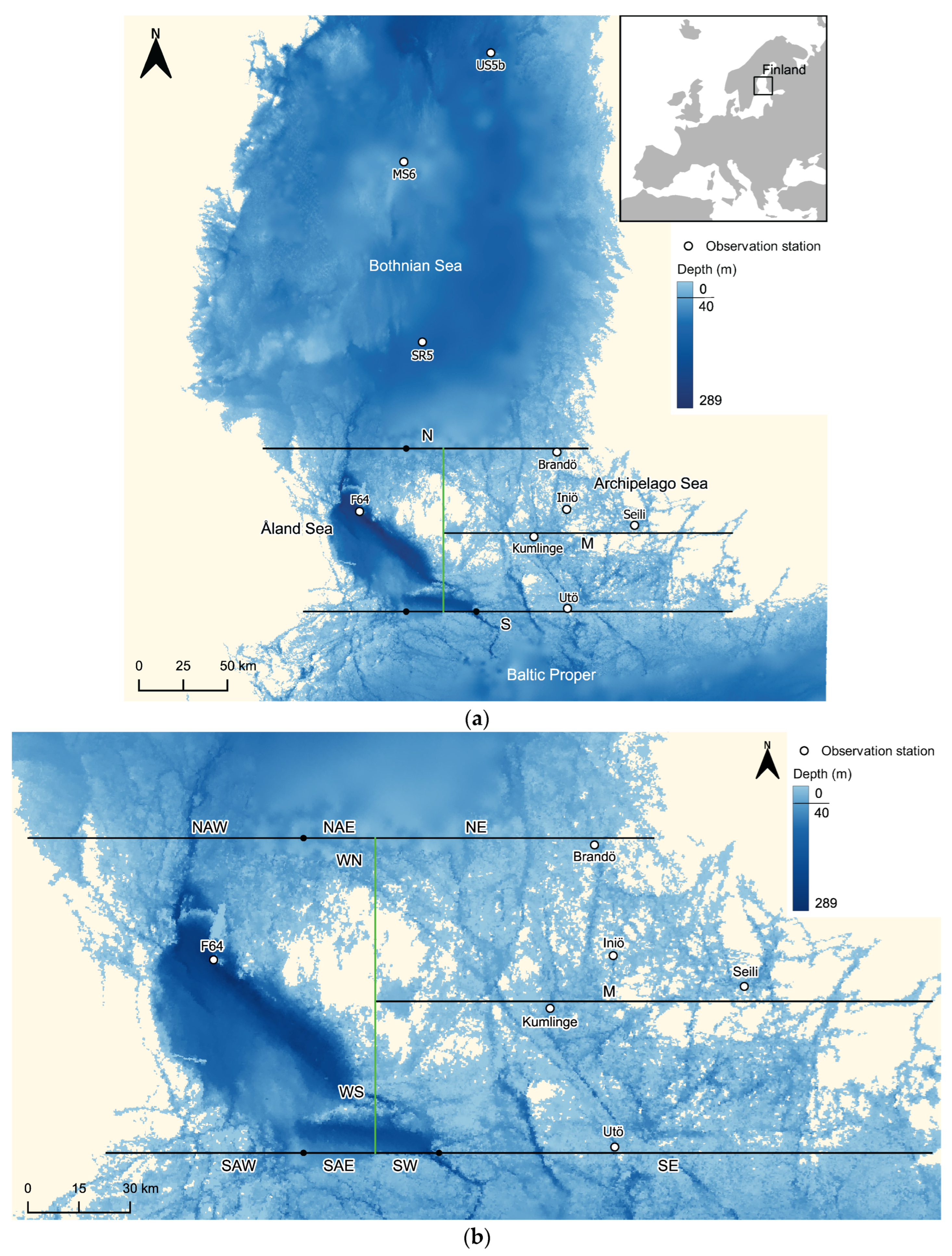
The Archipelago Sea is located between the Baltic proper and the Bothnian Bay (Figure 1). It is characterized by an enormous topographic complexity, including about 30,000 islands. The average water depth is only 23 m, and the deepest trench reaches 146 m. The total coastal drainage area is about 8900 km2 (of which lakes cover under 2% and fields cover 28%). The total area of the Archipelago Sea is about 9500 km2, and the water volume is 213 km3. The sea is non-tidal and characterized by a strong seasonality, including high summer temperatures and a more than 90% probability of annual ice cover during winter. Eight rivers run into the Archipelago Sea. The amount of water brought to the sea by the rivers is approximately 2.2 km3/a. The mosaic morphology and the environmental gradients (e.g., salinity, temperature, exposure) create several biotopes and complicated ecological webs [13,14]. As the topography is complex and the water shallow, the area acts as a buffer or filter between the coastline and the open sea and also between the Baltic proper and the Bothnian Bay. A great amount of suspended matter and nutrients settles down to the bottom, but the greater part of the nutrients is used for primary production [3].
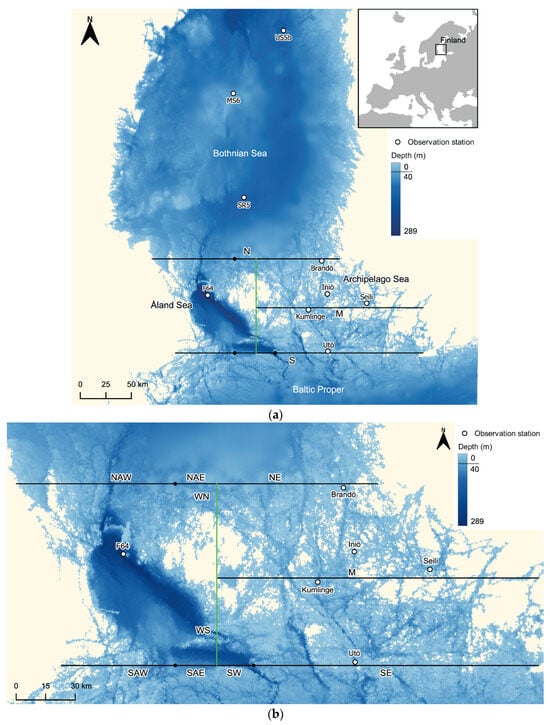
Figure 1.
(a) Model domain and the marine areas involved in this study. (b) A more detailed map of the main focus area. Sub-basins and sill areas relevant for the analysis are shown. The locations of stations and transects mentioned in the text are indicated. Coordinates (ETRS-TM35FIN) for the transects: Northern N6734237, Middle N6686155, Southern N6641527. Border line (green) between the Åland Sea and the Archipelago Sea E112442.
The Åland Sea is a sea area belonging to the Baltic Sea, located between the coast of Sweden and the mainland of Åland (Figure 1). It is 200–300 m deep in the north and shallower in the south. Between these depths, there is a threshold running across the sea at a depth of 70–80 m. The narrowest point is called the Åland Strait. The following definition is often used for the boundaries of the Sea of Åland: the southern boundary of the sea follows the latitude 59°50′ N, and the northern boundary follows the latitude 60°30′ N. The western boundary is along the eastern coast of Sweden, and the eastern boundary follows the western coastline of the main island of Åland and at sea, the longitude being 20° E.
2.2. 3-D Model
The Baltic Sea, like other sea areas, is simple a fluid that can be described to a good approximation by the primitive equations, i.e., the Navier–Stokes equations along with a nonlinear equation of state, which couple active tracers (temperature and salinity) to the fluid velocity.
The modelling configuration here is based on the Copernicus regional reanalysis data, which assimilate the NEMO4.0 model [15] simulations, satellite sea surface temperature and in situ temperature and salinity profiles. The primitive equation model is adapted to regional circulation problems down to a 1 nautical mile scale. In the horizontal direction, the model uses a curvilinear orthogonal grid, and in the vertical direction, it uses a full or partial step z-coordinate. The model setup used the z∗ vertical coordinate system. There were 56 vertical levels. The level thickness increased with the depth, being 1 m at the surface and about 20 m at the very bottom. All procedures are described in the quality information document of BALTICSEA_MULTIYEAR_PHY_003_011 [16]. This document also contains a detailed description of the validation and verification of the model product and its results. The physical system is validated against available observations such as in situ measurements and remote sensing data from Copernicus as well as observations from external sources [16]. All validation results will be uploaded and displayed on the BOOS webpage (http://www.boos.org/cmems-baltic-mfc-product-quality-information-multi-year-product/ (accessed on 1 January 2024). The model uses the CMEMS Northwest Shelf multi-year product as the western boundary [17], the ERA5 dataset for meteorological forcing [18] and the EHYPE model for river discharges [19].
As a result, averages of the 3D temperature, salinity, current fields, sea surface height and volume transports were saved once a day. Volume transports from the model were computed for a number of transects (Figure 1). These were integrated over the whole transect to calculate a time series.
The Åland Sea–Archipelago Sea model template has a horizontal resolution of 1 nautical mile (1.852 km), and it covers the area between 59.84 and 60.59° N and borders Sweden to the west and, similarly, Finland to the east (Figure 1).
2.3. Calculations
We calculated volume transports from the model results for three horizontal transects: Southern (S), Middle of the Archipelago Sea (M) and Northern (N) (Figure 1). The southern transect was further subdivided into SAW, SAE, SW and SE. The northern transect was correspondingly subdivided into NAW, NAE and NE. Furthermore, there was one vertical transect which separated the Åland Sea from the Archipelago Sea. It was divided into south to WS and in north to WN parts. The volume transports from the Copernicus fields were modified so that they were consistent with the average sea level of the subareas. To calculate a time series, we integrated the volume transports over the whole transect. Net flows (+ or −, km3) were calculated using the model separately for each month for the years 2000–2021. Water balances were calculated from the monthly results separately for the winter period (1 January–15 May and 15 October–31 December) and the summer period (16 May–14 October).
Water exchanges from the Baltic Proper to the Bothnian Sea through the Åland Sea were estimated in the northern boundary (N = NAW + NAE + NE) in the surface layer (0–40 m) and in the deep layer (over 40 m). In the Archipelago Sea, the surface layer extended up to 20 m, and the bottom layer was deeper than 20 m. The water balance was first calculated separately for different water layers in the southern and northern areas, and then they were combined. By doing this, we were able to estimate how much water (km3) moved from the deep layer to the surface at different times and in different parts of the Archipelago Sea.
Phosphorus fluxes were calculated from modeled water flows and water balances by considering the total phosphorus concentrations (µg/L) at different transects and interfaces. The data used for the calculations are described in the following paragraph, and the concentrations used for different periods are presented in the results in Table 1.

Table 1.
Inflows (t/a) of total phosphorus from the Baltic Proper to the Bothnian Sea and outflows (t/a) for vice versa through the Åland Sea in the years 2000–2021.
2.4. Water Quality Data
The water quality of the Archipelago Sea, the Åland Sea and the Bothnian Sea has been monitored since the 1960s with standard methods by environmental authorities, and the results are available from the open data service of Finnish Environment Institute (SYKE). Our mass balance calculations are based on total phosphorus (TP) concentrations. The water quality analysis here is based, in addition to total phosphorus concentrations, on dissolved inorganic phosphorus (DIP) concentrations in winter and algae production-related chlorophyll a concentrations in the surface water during the ecological classification period (1 July–7 September).
The total phosphorus concentration data for the nutrient flow budget through the Åland Sea is from station F64 (Figure 1). Every year, averages were calculated separately for the winter season (1 January–15 May and 15 October–31 December) and for summer (16 May–14 October) and separately for the surface layer (0–40 m) and bottom layer (40–100 m).
In the Archipelago Sea, the data were from stations Utö (S), Kumlinge (M) and Brändö (N) (Figure 1). Every year, the averages were calculated separately for the winter season (1 January–15 May and 15 October–31 December) and for summer (16 May–14 October) for the surface layer (0–20 m) and bottom layer (over 20 m). In addition, total phosphorus concentrations were calculated for the boundary between the surface and bottom layers as the average for depths of 20–40 m. Data from the Utö station were used for the section between the southern border and the middle border, and data from the Kumlinge station were used for the section between the middle border and the northern border. These concentrations were used to estimate how much phosphorus is transported from the deeper layers to the surface layer by currents.
Since data for the entire period (2000–2021) were not available from all observation stations, some of the phosphorus concentration data had to be generated using regression equations, as follows: For Utö (winter, surface) for the years 2010 and 2015–2021, TPws = 0.8919 TPss + 10.745, where TPss is the Utö (summer, surface; years 2000–2009 and 2011) phosphorus concentration (p = 0.01, R2 = 0.41). For Utö (winter, boundary layer 20–40 m) for the years 2010, 2012 and 2016–2021, TPwb = 0.5135 TPss + 16.011, where TPss is the Utö (summer, surface; years 2000–2009, 2011, 2013, 2014) phosphorus concentration (p = 0.01, R2 = 0.40). Even though the explanatory power of the equations appears to be quite low, both applied regressions are statistically significant (p = 0.01). For the regression line equation TPws = 0.8919 TPss + 10.745, the mean of TPws is 29.1, the mean of standard error (SE) for the data (n = 15) is 1.137 and the 95% confidence interval is, on average, 2.23. The magnitude of uncertainty can thus be estimated to be only about ±7.7% (2.23/29.1), and it does not significantly weaken the reliability of the estimates obtained by interpolation.
2.5. Additional Climatic Information
The North Atlantic Oscillation (NAO) index is based on the surface sea-level pressure difference between the Subtropical (Azores) High and the Subpolar Low. The NAO index is frequently used in climate-related studies. In the Baltic Sea region, the NAO is often applied as a proxy for the large-scale circulation that controls the local climate and is related to physical, chemical and biological processes. A positive, high index is associated with strong westerlies and anomalous warm temperatures in northern Europe [20]. The monthly values of the NAO index since 1950 can typically be found on the NOAA (National Oceanic and Atmospheric Administration) website or other climate data databases.
The seasonal sea water surface temperature anomalies from the 1991 to 2020 average for a specific area (58° N–63° N, 16° E–22° E) in the Baltic from 1980 to 2023 were downloaded from Climate Reanalyzer (Climate Change Institute, University of Maine (US), https://climatereanalyzer.org/research_tools/monthly_tseries/ (accessed on 10 December 2023).
3. Results
3.1. Through the Åland Sea
The inflow of water from the Baltic Proper to the Bothnian Sea occurs through the Åland Sea in the deep layer over 40 m, while the outflow occurs vice versa in the surface under 40 m. The inflow water volume from the Baltic Proper to the Bothnian Sea was estimated based on modeling results to be an average of 669 km3/a in the years 2000–2021. The outflow to the Baltic Proper was correspondingly 879 km3/a. The difference between the inflow and outflow, 210 km3/a, corresponds to the annual water volume of the rivers flowing into the Gulf of Bothnia.
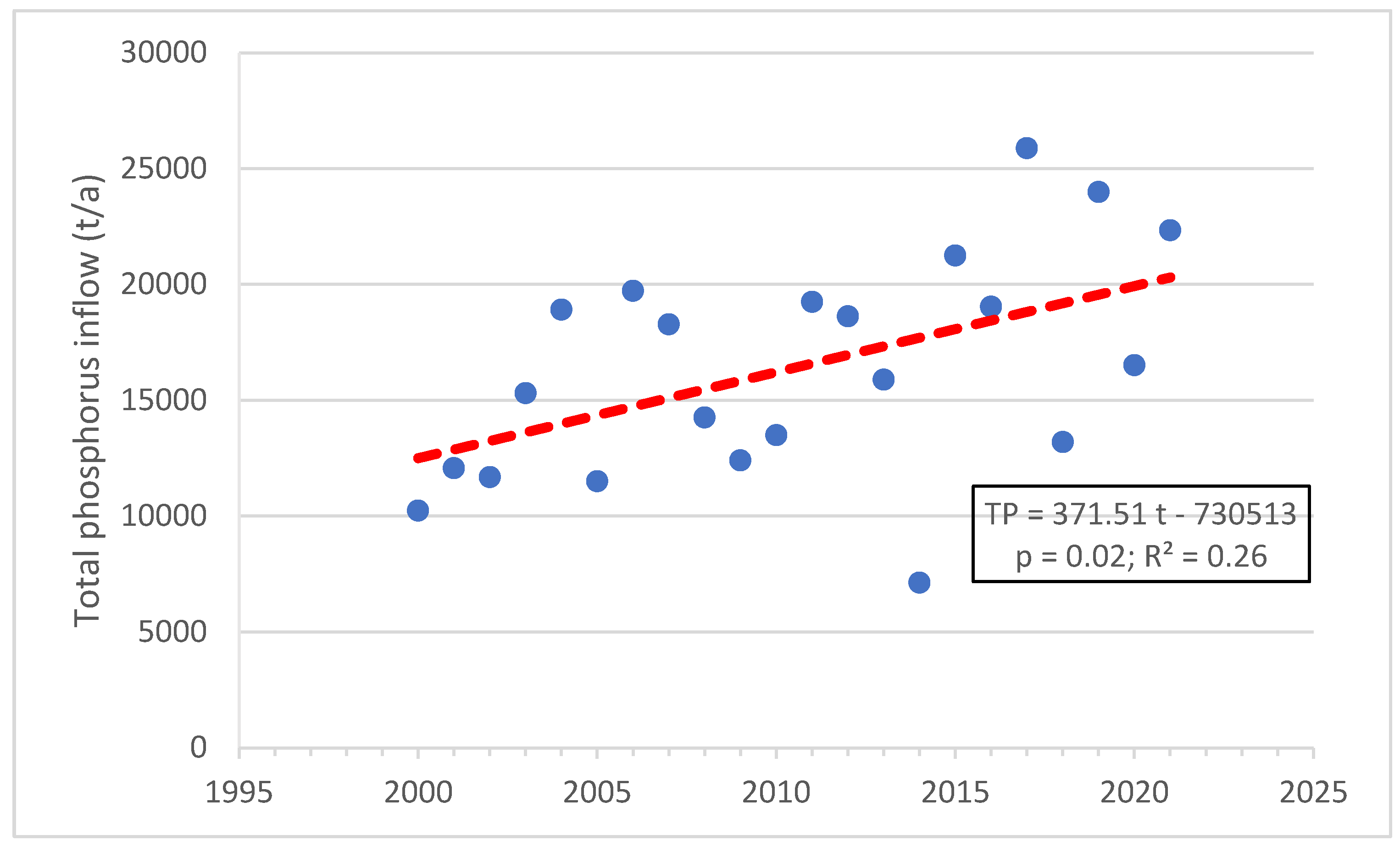
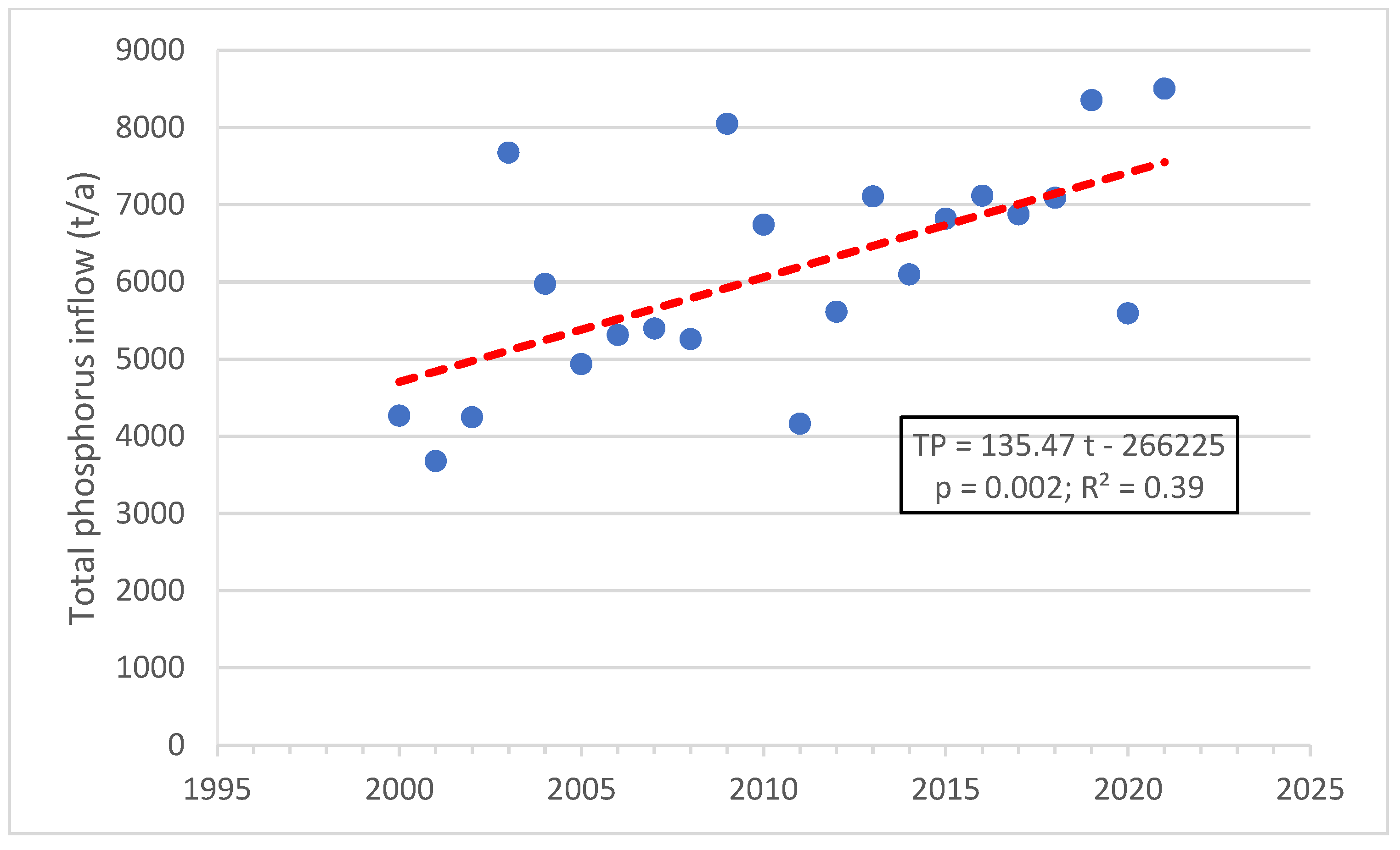
The amount of phosphorus carried by currents from the Baltic Proper to the Gulf of Bothnia has nearly doubled in the 2000s (Figure 2). In the years 2000–2002, 11,327 tons per year of phosphorus flowed into the Gulf of Bothnia from the main basin, and in the years 2019–2021, it was already 20,943 tons per year. The increase in phosphorus levels has been statistically significant both in the annual averages (p = 0.02) and especially during the summer months (p = 0.02) (Figure 3). In the 2000s, there was also a greater amount of phosphorus carried away in the water flowing out of the Gulf of Bothnia (Table 1). Therefore, the remaining amount (the difference between the inflow and outflow) does not seem to have changed much.
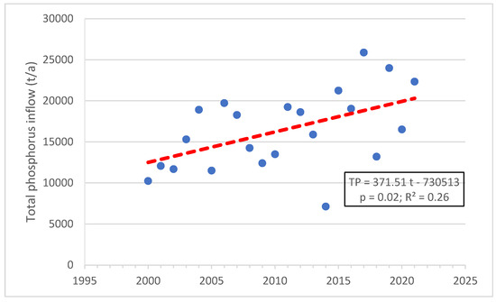
Figure 2.
The inflow of total phosphorus (t/a) from the Baltic Proper to the Bothnian Sea through the Åland Sea in the years 2000–2021. The red dashed line indicates the increasing trend (p = 0.02; R2 = 0.26).

Figure 3.
The inflow of total phosphorus (t/a) from the Baltic Proper to the Bothnian Sea through the Åland Sea in the summer season (16 May–14 October) in the years 2000–2021. The red dashed line indicates the increasing trend (p = 0.002; R2 = 0.39).
3.2. Water Flows in the Archipelago Sea
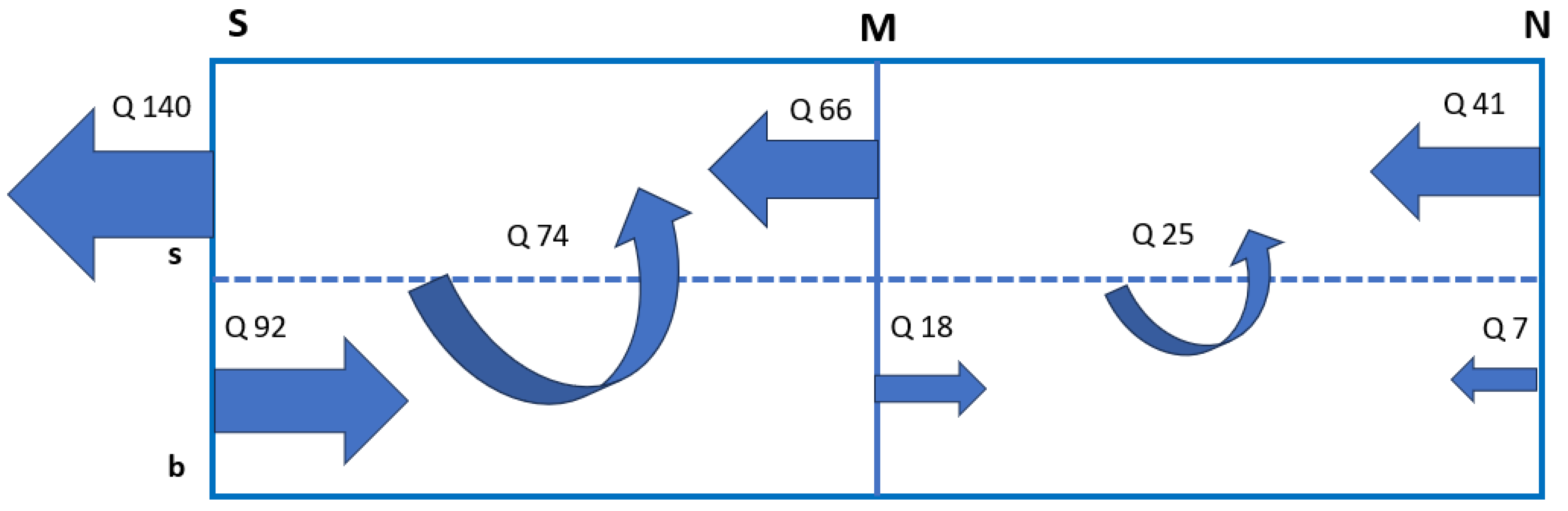
The surface and bottom currents were oriented from south to north in the Archipelago Sea in the years 2000–2014 (Figure 4 and Figure 5). In the years 2000–2009, the amount of water flowing into the surface layer (0–20 m) was 12 km3, and the amount of water flowing out at the northern edge was 56 km3. The difference of 44 km3 was water that came from deeper water layers (over 20 m) to the surface layer (Figure 4). Correspondingly, in the years 2010–2014, 87 km3 of water flowed into the surface layer and 140 km3 flowed out from the northern edge. A total of 53 km3 of water came from deeper layers into the surface layer (Figure 5).
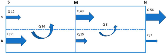
Figure 4.
Hydrological balance in different parts of the Archipelago Sea in the years 2000–2009. Q = net flow km3/a, S = southern transect, M = middle, N = northern, s = surface layer (0–20 m), b = bottom layer (over 20 m). Arrows indicate the directions of flows.
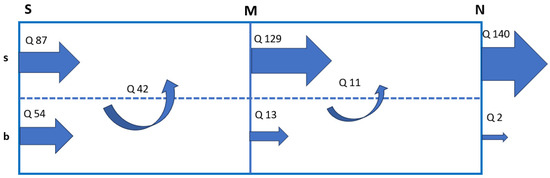
Figure 5.
Hydrological balance in different parts of the Archipelago Sea in the years 2009–2014. Q = net flow km3/a, S = southern transect, M = middle, N = northern, s = surface layer (0–20 m), b = bottom layer (over 20 m). Arrows indicate the directions of flows.
But after 2015, the situation changed, and the net flow in the surface layer reversed southwards in the Archipelago Sea (Figure 6). Between 2015 and 2021, water flowed into the surface layer of the Archipelago Sea from the northern edge at 41 km3 and exited from the southern edge at 140 km3. In the deeper water layer, water rose to the surface in the northern part (N-M) at 25 km3 and in the southern part (S-M) at 74 km3. In the deeper water layer, water continued to flow from the south to the Archipelago Sea at 92 km3, but the majority of it (80%) returned back towards the main basin in the surface layer.
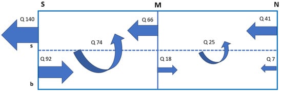
Figure 6.
Hydrological balance in different parts of the Archipelago Sea in the years 2015–2021. Q = net flow km3/a, S = southern transect, M = middle, N = northern, s = surface layer (0–20 m), b = bottom layer (over 20 m). Arrows indicate the directions of flows.
3.3. Phosphorus Flows in the Archipelago Sea
The net fluxes of total phosphorus have been similar to the general water flows in the Archipelago Sea in the 2000s. Although during the summer of 2000–2009, water and phosphorus flowed from the southern edge of the Archipelago Sea towards the main basin of the Baltic Sea, the net phosphorus load was still positive at that time (Table 2). Water balance calculations showed that compensating water from below the surface layer, with significantly higher phosphorus concentrations than at the surface, rose to the surface. In winter, the net water and phosphorus fluxes throughout the Archipelago Sea were directed from south to north. The average annual net phosphorus load, or the so-called background load, in the surface layer in 2000–2009 was calculated to be 485.7 t. Of this, 120.1 t occurred during the summer in the southern part of the Archipelago Sea (Table 3).
Table 2.
Phosphorus fluxes in different periods in the Archipelago Sea in the surface layer (0–20 m) in the summer season (s; 16 May–14 October) and in winter (w; 1 January–15 May and 15 October–31 December). South = southern transect (lat 59.84), Middle = middle transect (lat 60.14), North = northern transect (lat 60.59), S-M interface = horizontal boundary of the surface and bottom layer in 20 m in the sea area between the southern and middle transects. M-N interface = horizontal boundary of the surface and bottom layers in 20 m in the sea area between the middle and northern transects. Q = transport of water through the transects or interface (km3). A positive flow indicates a direction towards the north at the southern (S) and central (M) boundaries and a direction towards the south at the northern boundary (N). P = total phosphorus content of water in the transect or interface (µg/L). MF = mass flow of phosphorus through the transect or interface (t).
Table 3.
Summary of net phosphorus fluxes (t) in the Archipelago Sea surface layer (0–20 m). South part = the Archipelago Sea area that extends from its southern border (S) to the middle border (M); North part = the Archipelago Sea area that extends from the middle border (M) to the northern border (N).
From 2010 to 2014, the net fluxes of water and phosphorus throughout the Archipelago Sea were directed from south to north in both the summer and winter (Table 2). Although the water volumes were especially larger in winter compared to previous years, the average annual net phosphorus load was about 12% lower than in the early 2000s. The background phosphorus load in the surface layer for the years 2010–2014 was calculated to be 425 t, with 122.5 t occurring during the summer in the southern part of the Archipelago Sea (Table 3).
Since 2015, the net water flow in the surface layer of the Archipelago Sea turned southward. Correspondingly, phosphorus began to flow out from the southern Archipelago Sea with the surface currents towards the main basin of the Baltic Sea (Table 2). The average annual phosphorus outflow in the surface layer was calculated to be 182.2 t. The majority of this, 89% or 162.8 t, was transported out of the southern part of the Archipelago Sea during the summer (Table 3).
In summary, the situation regarding the background phosphorus load in the Archipelago Sea has changed significantly since 2015. Earlier in the 2000s, the net phosphorus load to the southern Archipelago Sea during the summer was around 120 t. According to modeling calculations, from 2015 to 2021, the net load had shifted to a phosphorus outflow of approximately 160 t during the summer.
3.4. Water Quality Time Series
In the Åland Sea, the total phosphorus concentrations of sea water (µg/L) in observation station F64 in the deep layer (40–100 m) have increased from 2000 to 2021 in summer statistically significantly (p = 0.003) (Figure 7). In wintertime (1 January–15 May and 15 October–31 December), the increasing trend is statistically indicative (p = 0.054). Inflow to the Bothnian Sea occurs in the deep layer.
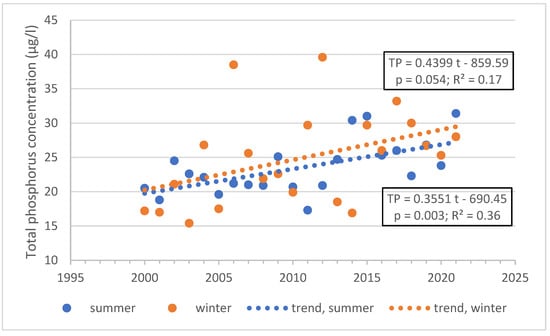
Figure 7.
Total phosphorus concentrations of sea water (µg/L) in observation station F64 in the Åland Sea in the deep layer (40–100 m). The blue dashed line indicates the increase in the TP concentration from 2000 to 2021 in summer (p = 0.003; R2 = 0.36), and the orange dashed line indicates that in winter (p = 0.054; R2 = 0.17).
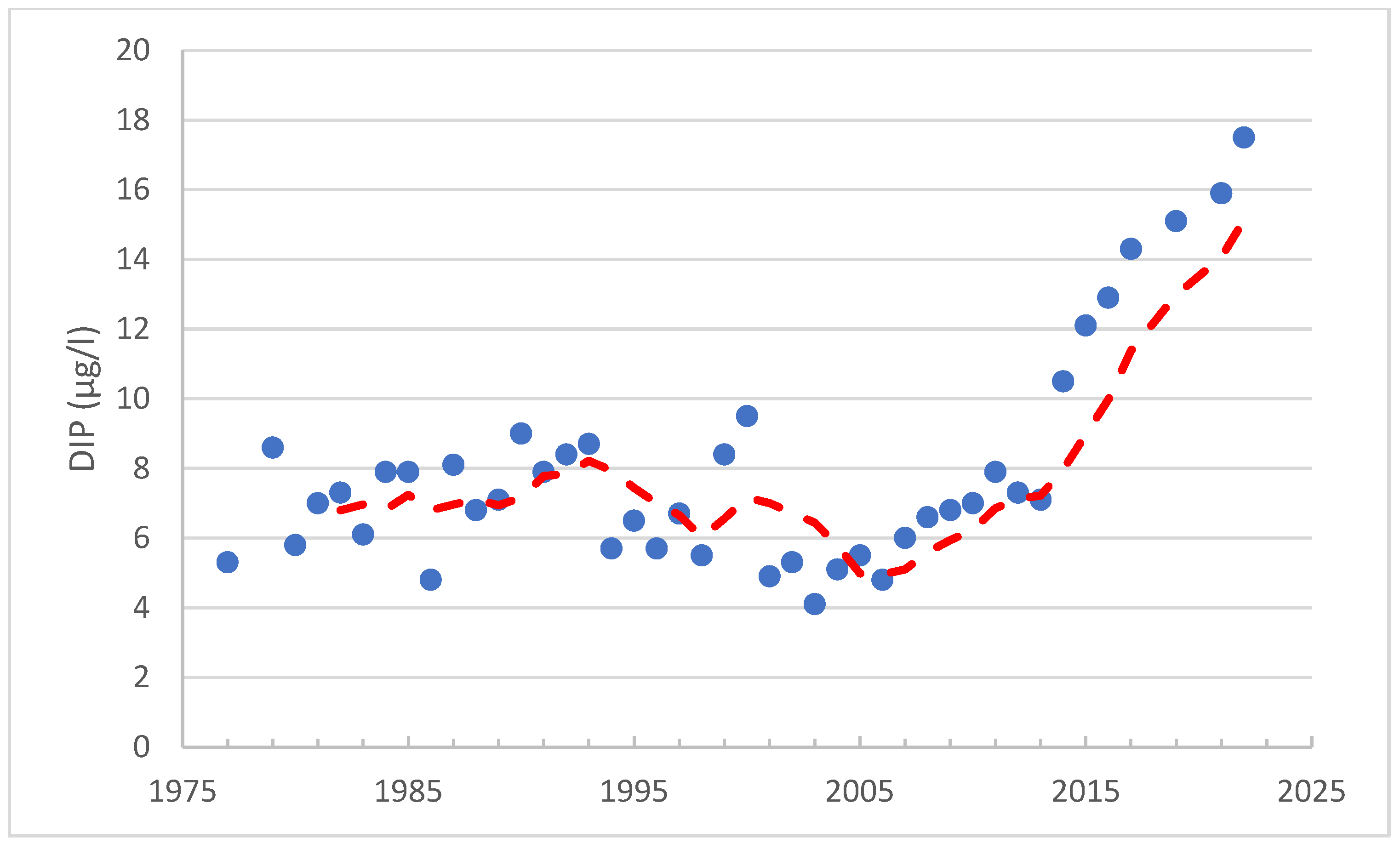
The observation stations SR5, MS6 and US5b are located in the open sea area of the Bothnian Sea (Figure 1). There, the wintertime (1 January–31 March) phosphate phosphorus concentration (DIP) in the surface layer of seawater has approximately doubled over the past ten years (Figure 8). The increasing trend from 2012 to 2022 has been statistically significant (p < 0.001; R2 = 0.92).
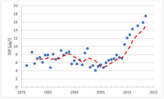
Figure 8.
The annual average concentration of phosphate phosphorus (DIP) at observation stations US5b, MS6 and SR5 in the surface layer during the winter season (1 January–31 March). The red dashed line represents the 5-year moving average.
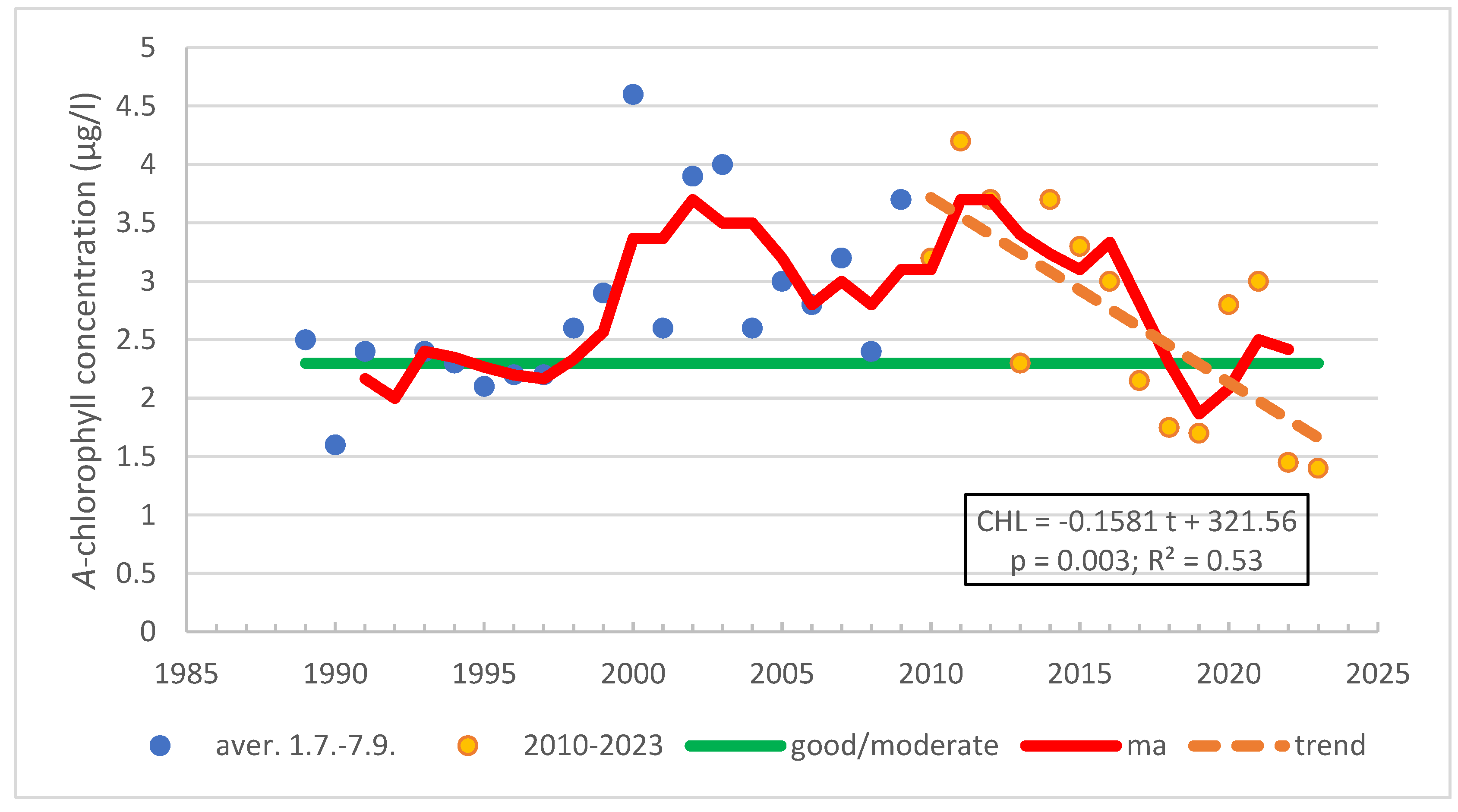
The observation station Iniö 33 is located in the southern part of Kihti in the middle of the Archipelago Sea (Figure 1). The chlorophyll a concentration in the surface water has varied significantly during the measurement period from 1989 to 2023 (Figure 9). From 1989 to 1999, it remained, on average, at the good threshold level (2.3 µg/L, according to water frame directive ecological classification), after which it rose noticeably. The average chlorophyll concentration from 2000 to 2009 was 3.3 µg/L, and from 2009 to 2012, it was already 3.7 µg/L. From that level, the chlorophyll a concentration began to decrease to its current values: from 2018 to 2023, the average was only 2.0 µg/L, indicating a good status had been achieved. The decrease observed from 2010 to 2022 was statistically significant (p = 0.003).
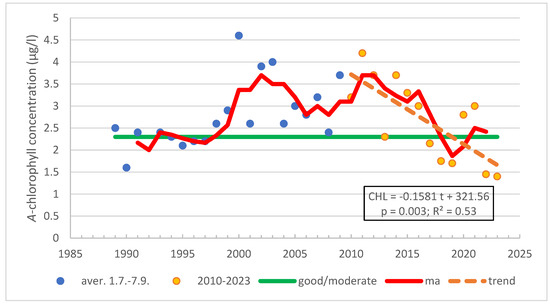
Figure 9.
The concentration of chlorophyll a (µg/L) in surface water (0–10 m) at observation station Iniö 33 during the ecological classification period (1 July–7 September) from 1989 to 2023. The good status threshold (good/moderate) is 2.3 µg/L. The red line represents the three-year moving average of the chlorophyll concentration. The orange dashed line indicates the decrease in the chlorophyll concentration from 2010 to 2023 (p = 0.003; R2 = 0.53).
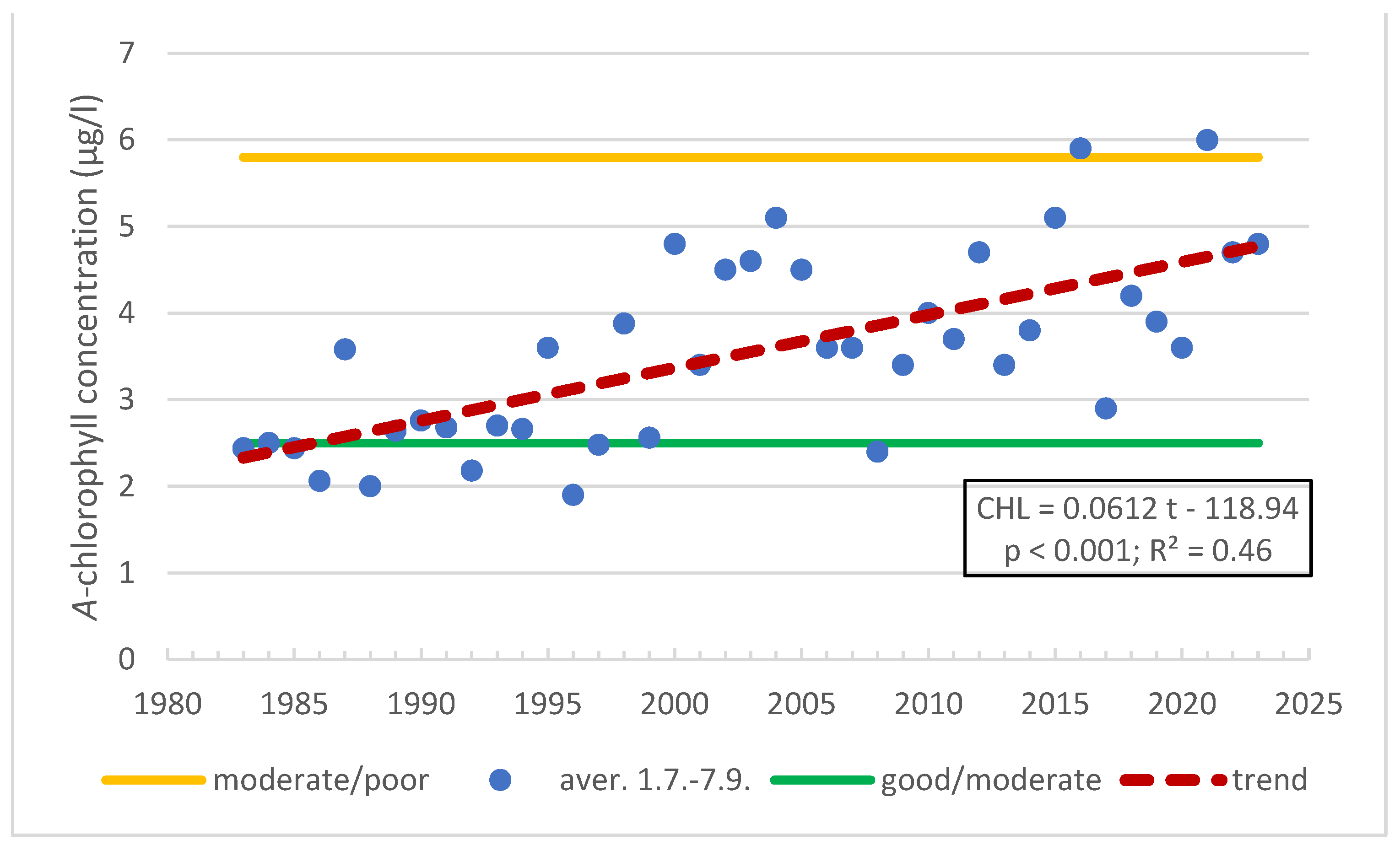
The development of water quality has been different at the Seili intensive station, which is located in the southern part of Airisto, closer to the coast and about 30 km from the city of Turku. There, the chlorophyll a concentration has steadily increased by approximately 0.6 µg/L per decade since 1983 during the ecological classification period (1 July–7 September) (Figure 10). The deteriorating trend is statistically significant (p < 0.01). At the beginning of the series, the chlorophyll a concentration was close to the good status threshold (2.5 µg/L), but it has now reached a level of 5 µg/L, which is close to the poor status threshold (5.8 µg/L).
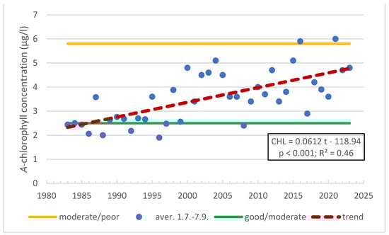
Figure 10.
The concentration of chlorophyll a (µg/L) in surface water (0–10 m) at observation station Seili during the ecological classification period (1 July–7 September) from 1983 to 2023. The good status threshold (good/moderate) is 2.3 µg/L, and the moderate (moderate/poor) one is 5.8 µg/L. The red dashed line indicates the increase in the chlorophyll a concentration over the entire period under review (p < 0.001; R2 = 0.46).
3.5. Climatic Observations
The annual NAO index was practically zero during the period from 2000 to 2021. During wintertime (1 January to 30 April and 1 November to 31 December), it was positive, with an average of 0.357, and during summertime (1 May to 31 October), it was negative, with an average of −0.371. From 2015 to 2021, the NAO index during winter was significantly higher than the average for the 2000s, at 0.676 (Figure 11). During the same period, the annual index turned positive: from 2000 to 2014, the average was −0.095, while from 2015 to 2021, it was 0.183.
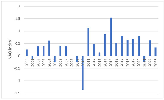
Figure 11.
Values of the NAO index in winter (1 January to 30 April and 1 November to 31 December) in the years 2000–2023.
The surface water of the Baltic Sea has warmed by approximately 1.7 °C over the past 40 years (Figure 12). Based on the moving average, since 2015, the temperature increase has been particularly rapid, at up to 0.1 °C per year.
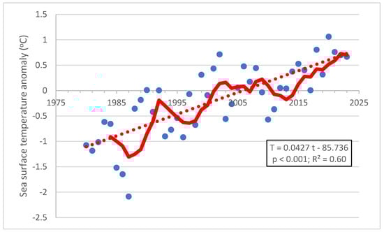
Figure 12.
Seasonal sea water surface temperature anomalies from the 1991 to 2020 average for the specific area (58° N–63° N, 16° E–22° E) in the Baltic from 1980 to 2023 in the summer season (1 May to 31 October). The red line is the 5-year moving average, and the red dashed line is a linear and statistically significant increasing trend (p < 0.001; R2 = 0.60).
4. Discussion
In this study, seawater flows in the Archipelago Sea and the Sea of Åland were calculated using 3-D modeling. Additionally, phosphorus fluxes and its net loads were investigated. Mass balance calculations were performed for total phosphorus. In the marine phosphorus (P) cycle, dissolved inorganic phosphorus (DIP), particulate inorganic (PIP) and organic phosphorus (POP) and dissolved organic phosphorus (DOP) are the main P pools. DIP is consumed by phyto- and bacterioplankton, incorporated into biomass, forming POP, and, following cell death and remineralization, partly released as DOP into the surrounding water. DOP acts as an additional P source to microbial organisms, especially when it dominates the dissolved P pool [21]. Total phosphorus (TP) was here used as a proxy for nutrients available to the planktonic organisms. The basis for this assumption was that in a nutrient-constrained environment with significant turnover of N and P, like during the summer season in the northern Baltic Sea, inorganic nutrients are rapidly (within hours) assimilated by the organisms [22].
Phosphorus is a growth-limiting nutrient for phytoplankton in the Baltic Sea. According to the earlier studies [23] from the Archipelago Sea, phosphorus limited phytoplankton growth, especially in spring and in summer, while nitrogen was the limiting factor in late summer and in autumn. But a shift from production limitation by both nutrients to limitation by nitrogen alone has obviously occurred because the phosphorus concentrations of the sea water in the Archipelago Sea have increased. On the other hand, the Archipelago Sea receives a strong surplus of nitrogen, TN:TP = 14,7 [8]. For atmospheric deposition, the ratio TN:TP = 54 [24]. Therefore, its transport by sea currents from other sea areas to the Archipelago Sea is not necessarily as interesting as that of phosphorus. In this context, we also analyzed changes in water quality in relation to observed phosphorus fluxes. The chlorophyll-a concentration, which indicates algal production during the ecological classification period, was used as a variable for water quality. It is essentially a composite variable that reflects the effects of various growth-limiting factors. Changes in the water quality of the open Bothnian Sea are assessed based on the concentrations of dissolved phosphorus (DIP). Winter nutrient concentrations are used as one indicator of eutrophication when assessing the state of the Baltic Sea. High winter phosphorus concentrations predict abundant cyanobacterial blooms in the summer.
The inflow water volume from the Baltic Proper to Bothnian Sea was estimated in our modeling in the years 2000–2021 to be an average of 669 km3/a, and the outflow was 879 km3/a. Håkansson et al. [25] gave water flux estimates of the same magnitude: a 750 km3/a inflow and 1055 km3/a outflow based on mass-balance modeling for salt. However, our estimates are about 30% smaller than those calculated by Yi et al. [26], with an inflow of 980 km3/a and an outflow of 1180 km3/a. They calculated based on a mass balance model for 129I in the Baltic Proper and the Bothnian Sea and covered only the period from November to December 2009. Here, 129I refers to Iodine-129, which is a long-lived radioisotope of iodine. The estimates by Yi et al. [26] are in line with previous assessments made by Fonselius [27] (inflow of 900 km3/a and outflow of 1100 km3/a) and by Wulff et al. [28] (inflow of 1000 km3/a and outflow of 1223 km3/a). Savchuk [29] estimated that the water flows between the Baltic Sea basins averaged over 1991–1999 would have been 1009 km3/a and 1237 km3/a. The uncertainty range estimates of Yi et al. [26], 600–1400 km3/a for the inflow and 780–1600 km3/a for the outflow, also lie within the ones given by Wulff et al. [28] (inflow: 687–1912 km3/a, outflow: 508–1673 km3/a). In our study, for the inflow, the minimum was 262 km3/a, and the maximum was 897 km3/a; correspondingly, for the outflow, the range was 521–1110 km3/a. The minimum inflow and outflow were recorded in the year 2014.
One reason for the discrepancies in the estimates of water volumes in inflows and outflows can be found in the methods used. The majority of earlier estimates are based on various balance calculations, and the examination timeframes vary greatly. The only modern 3-D hydrodynamic modeling calculations have been presented in the publications by Westerlund et al. [30] and Miettunen et al. [11], but for some reason, they arrive at a conclusion significantly different from those in previous studies. These models covered the years 2013–2017. According to Westerlund et al. [30], the mean volume transports for the MS transect for the whole modelling period would have been −24,000 m3 s−1 (whole water column), −33,000 m3 s−1 (upper layer) and 9200 m3 s−1 (lower layer). These estimates (inflow: 290 km3/a; outflow: 1041 km3/a), taking into account the river flows (about +200 km3/a), would mean that the Gulf of Bothnia would empty out gradually at a rate of about 550 km3/a. Miettunen et al. [11] arrived at the same estimate: averaging over our study period of 2013–2017, the mean of the net transport over the northern Archipelago Sea transect is −206 km3 per year. This is approximately 28% of the mean net transport over the Åland Sea transect, which was −745 km3 per year.
Our estimation of the inflow flux of total phosphorus from the Baltic Proper to the Bothnian Sea in the years 2000–2021, 16,400 t/a, is about 26% smaller compared to the estimates made in other studies (Table 4). Correspondingly, our outflow flux estimate, 13,100 t/a, is about 14% smaller. According to our model, the phosphorus flux increased in both the inflow and outflow during the 2000s and was 20,300 t/a (inflow), and the outflow was 17,800 t/a (outlow) during the years 2015–2021. During these years, the difference compared to other estimates was −20% in the inflow and +17% in the outflow.
Table 4.
Comparison to earlier estimates of the inflow flux of total phosphorus from the Baltic Proper to the Bothnian Sea (IF TP; t/a), the outflow flux from the Bothnian Sea to the Baltic Proper km3/a (OF TP; t/a), the inflow water volume from the Baltic Proper to the Bothnian Sea (IF Wa; km3/a) and the outflow OF Wa (km3/a).
Different previous estimates of phosphorus flows between the main basin of the Baltic Sea and the Bothnian Sea vary quite a lot. The reason for the variation is the different methods of calculating the water volumes and the concentration estimates used. For example, in both of Savchuk’s articles [29,31], the same water balance was used (an inflow of 1009 km3/a and an outflow of 1237 km3/a [29]), so the phosphorus concentrations during the calculation periods determined the flow estimate. In the first study [29], the phosphorus concentration of the inflowing water was 32.7 µg/L, and in the second [31], it was 30.1 µg/L. These were clearly (more than 20%) higher concentrations than what was measured as the averages from depths of 40–100 m at observation station F64 in the 2000s: 23.5 µg/L in summer and 24.9 µg/L in winter. In Savchuk’ studies [29,31], the Data Assimilation System was used for the reconstruction of the temporally averaged means and integral mounts of nutrients and hydrographic variables in the different areas of the Baltic Sea. Yi et al. [26], on the other hand, calculated phosphorus fluxes of 20,000 t/a and 12,000 t/a with phosphorus concentrations of 20 µg/L (inflow) and 10 µg/L (outflow), which were assigned to inflow and outflow water, respectively, for the period 1997–2005 by Håkanson and Bryhn [25]. According to their article [25], the fluxes between the Baltic Proper (BP) and the Bothnian Sea (BS) are calculated using data on TP-concentrations from the Bothnian Sea and data from 1997 to 2005 for the surface-water layer down to 42 m in the Bothnian Sea.
For our water exchange analysis in the Åland Sea, transports were integrated over the upper part of the water column down to a 40 m depth and over the lower part of the water column below a 40 m depth. This roughly split the water column into an upper (and intermediate) layer above the halocline and a deep layer below the halocline [30]. Our water quality data in situ is from station F64, located in the middle of the Åland Sea (Figure 1). At the station, there is a deep area with a depth of about 285 m, while the average depth of the Åland Sea is approximately 75 m. The phosphorus concentration of the surface layer was calculated as the average from depths of 0–40 m and, correspondingly, for the deep layer from 40–100 m. In the latter, the phosphorus concentrations represent the deep layer of the water column, which extends well beyond the average depth, but do not account for the water layer in the deepest area where water exchange occurs the least. In our opinion, the selected depths best represent the quality of the mixed water flowing southwards and northwards. Recently, Muchowski et al. [32] made observations of strong turbulence and mixing below the halocline in the sill of the Åland Sea. They concluded that the deep water below the halocline is likely modified along its way through the Åland Sea, which further supports our opinion.
We found that the amount of phosphorus carried by currents from the Baltic Proper to the Gulf of Bothnia nearly doubled in the 2000s. At the same time, the wintertime phosphate phosphorus (DIP) concentration in the open sea of the Gulf of Bothnia increased significantly (Figure 8). The increase in winter phosphate phosphorus concentrations is a sign of the growth of usable phosphorus stocks in the Gulf of Bothnia, where an increase in cyanobacterial blooms has been observed, especially in recent years. In winter, the available nutrients in the sea largely determine the abundance of spring microalgae blooms. The spring bloom initiates the growing season of the Baltic Sea ecosystem and is the most significant event in the annual nutrient cycle. The abundance of spring blooms correlates with the summer cyanobacterial blooms. The increased phosphorus flux in the Gulf of Bothnia is mainly due to the rise in phosphorus concentrations in the deep-water layers of the Åland Sea (40–100 m), which in turn is directly linked to changes in phosphorus concentrations in the main basin of the Baltic Sea.
There is only one previous calculation of background nutrient loads for the Archipelago Sea based on a 3-D hydrodynamic model [4]. According to it, on average, net inflows of simulated nutrients, nitrogen and phosphorus occurred in 1993–1997; only in 1993 was a net outflow of nitrogen found. The amount of the nitrogen load was 12,300 t/a, and that of phosphorus was 580 t/a. The range for the P estimate was 139–992 t/a. According to this study, from 2000 to 2014, the net phosphorus load, or background load, averaged about 465 t/a, of which 120 t occurred during the summer. The annual net inflow of P was thus about 20% lower in the early 2000s than in the mid-1990s. During the same period, the total phosphorus load entering the Archipelago Sea (the river load and point load, excluding the atmospheric load and internal load) averaged 537 t/a (SYKE).
Starting in 2015, the surface currents and phosphorus flows made a U-turn and, contrary to previous patterns, began to move southward from the Archipelago Sea towards the main basin of the Baltic Sea. Based on the modeling, the annual outflow of phosphorus in 2015–2021 was estimated to be 182 t, of which 162 t occurred during the summer. At the same time, in the central part of the Archipelago Sea, the chlorophyll concentration began to decrease to its current values under 2.0 µg/L, indicating a good status had been achieved (Figure 9). The total phosphorus load entering the Archipelago Sea in 2015–2021 appears to have decreased by about 18% and averaged 442 t/a (SYKE). But these reductions in phosphorus loadings are not reflected in the inner or archipelago areas of the Archipelago Sea, where measured chlorophyll concentrations have been increasing steadily (Figure 10). The Archipelago Sea was still overall classified in a satisfactory ecological state in the WFD classification conducted in 2019. Near the coast, in the middle and inner archipelago, there are also water areas in poor and even bad conditions. The inner archipelago is mostly sheltered and is under major influence from local riverine inputs [10]. This indicates that the inner archipelago is mostly affected by local sources.
5. Conclusions
One of the most important results of this article was the observation of the change in the direction of surface currents in the Archipelago Sea. After the year 2015, the net flow in the surface layer reversed southwards in the Archipelago Sea. As a result, phosphorus also began to be removed from the surface layer of the Archipelago Sea towards the main basin of the Baltic Sea. The ongoing climate change may be influencing this U-turn in surface currents. In the climate analysis, we found indications of the strengthening of the NAO index around the same time when, according to the modeling, the direction of surface currents changed, and water began to upwell from the deeper water layer about twice as much as before (Figure 4, Figure 5 and Figure 6). The wintertime NAO rose to a value of 0.676, and the rate of warming of the surface water approximately doubled. An anomalous high NAO index (>0.5) reflects strong westerlies and is consequently related to warmer winters in the Baltic Sea region compared to anomalous low index years [20]. According to Lehmann et al. [33], in the Baltic Sea during NAO+ phases, strong Ekman currents are produced with increased up- and downwelling along the coasts and associated coastal jets, whereas during NAO− phases, Ekman drift and upwelling are strongly reduced. However, a more detailed understanding of the explanatory mechanisms behind the observations of this study requires more comprehensive analysis and also new modeling.
Author Contributions
Conceptualization, H.H. and A.I.; methodology, H.H. and A.I.; software, A.I.; validation, A.I.; formal analysis, A.I. and H.H.; investigation, H.H.; resources, H.H.; data curation, H.H.; writing—original draft preparation, H.H.; writing—review and editing, H.H.; visualization, H.H.; supervision, H.H.; project administration, H.H.; funding acquisition, H.H. All authors have read and agreed to the published version of the manuscript.
Funding
This research was funded by The Regional Council of Southwest Finland’s regional board. Support for the implementation of the project is granted under the Act on the Financing of Regional Development and European Union Regional and Structural Policy Projects (757/2021).
Institutional Review Board Statement
Not applicable.
Informed Consent Statement
Not applicable.
Data Availability Statement
Data supporting the reported results can be found at http://www.syke.fi/avoindata (accessed on 12 October 2023).
Acknowledgments
This study was conducted at the Centre for Economic Development, Transport, and the Environment, Turku (VARELY). The monitoring data were collected from databases in the VARELY and the Finnish Environment Institute (SYKE).
Conflicts of Interest
Author Arto Inkala was employed by the company AI Innovation Ltd. The remaining authors declare that the research was conducted in the absence of any commercial or financial relationships that could be construed as a potential conflict of interest.
References
- Andersen, J.H.; Carstensen, J.; Conley, D.J.; Dromph, K.; Fleming-Lehtinen, V.; Gustafsson, B.G.; Josefson, A.B.; Norkko, A.; Villnäs, A.; Murray, C. Long-term temporal and spatial trends in eutrophication status of the Baltic Sea. Biol. Rev. 2017, 92, 135–149. [Google Scholar] [CrossRef] [PubMed]
- Laamanen, M.; Suomela, J.; Ekebom, J.; Korpinen, S.; Paavilainen, P.; Lahtinen, T.; Nieminen, S.; Hernberg, A. Suomen merenhoitosuunnitelman toimenpideohjelma vuosille 2022–2027; Ympäristöministeriö: Helsinki, Finland, 2021. (In Finnish) [Google Scholar]
- Berninger, K.; Fleming, V.; Huttunen, M.; Iho, A.; Niskanen, L.; Kuosa, H.; Piiparinen, J.; Räike, A.; Salo, M.; Sarkkola, S.; et al. Rannikkovesille tuntuvia kuormitusvähennyksiä; Policy Brief No. 26; Valtioneuvoston selvitys- ja tutkimustoiminta: Helsinki, Finland, 2023. (In Finnish) [Google Scholar]
- Helminen, H.; Juntura, E.; Koponen, J.; Laihonen, P.; Ylinen, H. Assessing of long-distance background nutrient loading to the Archipelago Sea, northern Baltic with a hydrodynamic model. Environ. Model. Softw. 1998, 13, 511–518. [Google Scholar] [CrossRef]
- Hyytiäinen, K.; Huttunen, I.; Kotamäki, N.; Kuosa, H.; Ropponen, J. Good eutrophication status is a challenging goal for coastal waters. Ambio 2024, 53, 579–591. [Google Scholar] [CrossRef] [PubMed]
- Huttunen, I.; Huttunen, M.; Piirainen, V.; Korppoo, M.; Lepistö, A.; Räike, A.; Tattari, S.; Vehviläinen, B. A national-scale nutrient loading model for Finnish watersheds—VEMALA. Environ. Model. Assess. 2016, 21, 83–109. [Google Scholar] [CrossRef]
- Huttunen, I.; Hyytiäinen, K.; Huttunen, M.; Sihvonen, M.; Veijalainen, N.; Korppoo, M.; Heiskanen, A.-S. Agricultural nutrient loading under alternative climate, societal and manure recycling scenarios. Sci. Total Environ. 2021, 783, 146871. [Google Scholar] [CrossRef] [PubMed]
- Fleming, V.; Berninger, K.; Aikola, T.; Huttunen, M.; Iho, A.; Kuosa, H.; Niskanen, L.; Piiparinen, J.; Räike, A.; Salo, M.; et al. Rannikkovesien ravinteiden kuormituskatot ja kuormituksen vähentämisen keinoja: Loppuraportti; Valtioneuvoston selvitys-ja tutkimustoiminnan julkaisusarja: Helsinki, Finland, 2023; Volume 45. (In Finnish) [Google Scholar]
- Lignell, R.; Miettunen, E.; Tuomi, L.; Ropponen, J.; Kuosa, H.; Attila, J.; Puttonen, I.; Lukkari, K.; Peltonen, H.; Lehtoranta, J.; et al. Rannikon kokonaiskuormitusmalli: Ravinnepäästöjen vaikutus veden tilaan—Kehityshankkeen loppuraportti (XI 2015–VI 2018); Finnish Environment Institute: Helsinki, Finland, 2019. (In Finnish) [Google Scholar]
- Miettunen, E.; Tuomi, L.; Myrberg, K. Water exchange between the inner and outer archipelago areas of the Finnish Archipelago Sea in the Baltic Sea. Ocean Dynam. 2020, 70, 1421–1437. [Google Scholar] [CrossRef]
- Miettunen, E.; Tuomi, L.; Westerlund, A.; Kanarik, H.; Myrberg, K. Transport dynamics in a complex coastal archipelago. Ocean Sci. 2024, 20, 69–83. [Google Scholar] [CrossRef]
- Madec, G. and the NEMO System Team. NEMO ocean engine. Sci. Notes Clim. Model. Cent. 2019, 27, 1–323. [Google Scholar] [CrossRef]
- Bonsdorff, E.; Blomqvist, E.M. Biotic couplings on shallow water softbottoms—Examples from the northern Baltic Sea. Oceanogr. Mar. Biol. Annu. Rev. 1993, 31, 153–176. [Google Scholar]
- Von Numers, M. Distribution, numbers and ecological gradients of birds breeding on small islands in the Archipelago Sea, SW Finland. Acta Zool. Fennica 1995, 197, 1–127. [Google Scholar]
- Gurvan, M.; Bourdallé-Badie, R.; Chanut, J.; Clementi, E.; Coward, A.; Ethé, C.; Iovino, D.; Lea, D.; Lévy, C.; Lovato, T.; et al. NEMO Ocean engine. In Notes du Pôle de Modélisation; v4.0, Number 27; Institut Pierre-Simon Laplace (IPSL): Guyancourt, France, 2019. [Google Scholar] [CrossRef]
- Panteleit, T.; Verjovkina, S.; Jandt-Scheelke, S.; Spruch, L.; Huess, V. Quality Information, Document, Baltic Sea Production Centre, Issue 4.0. 2023. Available online: https://data.marine.copernicus.eu/product/BALTICSEA_MULTIYEAR_PHY_003_011/description (accessed on 30 November 2022).
- Copernicus Marine Service Information (CMEMS) North West Shelf multi-year, E.U. Atlantic—European North West Shelf—Ocean Physics Reanalysis. Marine Data Store 2023. Available online: https://data.marine.copernicus.eu/product/NWSHELF_MULTIYEAR_PHY_004_009/description (accessed on 12 February 2022).
- Hersbach, H.; Bell, B.; Berrisford, P.; Hirahara, S.; Horányi, A.; Muñoz-Sabater, J.; Nicolas, J.; Peubey, C.; Radu, R.; Schepers, D.; et al. The ERA5 global reanalysis. Q. J. R. Meteorol. Soc. 2020, 146, 1999–2049. [Google Scholar] [CrossRef]
- SMHI. EHYPE-Model System; Version: ehype3_fgd; SMHI: Norrköping, Sweden, 2020. [Google Scholar]
- Löptien, U.; Mårtensson, S.; Meier, H.E.M.; Höglund, A. Long-term characteristics of simulated ice deformation in the Baltic Sea (1962–2007). J. Geophys. Res. Ocean. 2012, 118, 801–815. [Google Scholar] [CrossRef]
- Nausch, M.; Achterberg, E.P.; Bach, L.T.; Brussaard, C.P.D.; Crawfurd, K.J.; Fabian, J.; Riebesell, U.; Stuhr, A.; Unger, J.; Wannicke, N. Concentrations and Uptake of Dissolved Organic Phosphorus Compounds in the Baltic Sea. Front. Mar. Sci. 2018, 5, 386. [Google Scholar] [CrossRef]
- Andersson, A.; Höglander, H.; Karlsson, C.; Huseby, S. Key role of phosphorus and nitrogen in regulating cyanobacterial community composition in the northern Baltic Sea. Estuar. Coast. Shelf Sci. 2015, 164, 161–171. [Google Scholar] [CrossRef]
- Kirkkala, T.; Helminen, H.; Erkkilä, A.A. Variability of nutrient limitation in the Archipelago Sea SW Finland. Hydrobiologia 1998, 363, 117–126. [Google Scholar] [CrossRef]
- Suomela, J. Kirkkaasta sameaan. Meren kuormitus ja tila Saaristomerellä ja Ahvenanmaalla; Varsinais-Suomen elinkeino-, liikenne-ja ympäristökeskuksen julkaisuja: Turku, Finland, 2011; Volume 6. (In Finnish) [Google Scholar]
- Håkanson, L.; Bryhn, A.C. Eutrophication in the Baltic Sea—Present Situation, Nutrient Transport Processes, Remedial Strategies; Springer: Berlin/Heidelberg, Germany, 2008; 261p. [Google Scholar]
- Yi, P.; Possnert, G.; Aldahan, A.; Hou, X.L.; Bryhn, A.C.; He, P. 129I in the Baltic Proper and Bothnian Sea: Application for estimation of water exchange and environmental impact. J. Environ. Radioact. 2013, 120, 64–72. [Google Scholar] [CrossRef]
- Fonselius, S. Om Österjöns och speciellt Botniska vikens hydrografi. Vatten 1971, 3, 309–324. [Google Scholar]
- Wulff, F.; Rahm, L.; Hallin, A.-K.; Sandberg, J. A nutrient budget model of the Baltic Sea. In A Systems Analysis of the Baltic Sea 2001; Wulff, F., Rahm, L., Larsson, P., Eds.; Springer: Berlin/Heidelberg, Germany, 2001; pp. 353–372. [Google Scholar]
- Savchuk, O.P. Resolving the Baltic Sea into seven subbasins: N and P budgets for 1991–1999. J. Mar. Syst. 2005, 56, 1–15. [Google Scholar] [CrossRef]
- Westerlund, A.; Miettunen, E.; Tuomi, L.; Alenius, P. Refined estimates of water transport through the Åland Sea in the Baltic Sea. Ocean Sci. 2022, 18, 89–108. [Google Scholar] [CrossRef]
- Savchuk, O.P. Large-Scale Nutrient Dynamics in the Baltic Sea, 1970–2016. Front. Mar. Sci. 2018, 5, 95. [Google Scholar] [CrossRef]
- Muchowski, J.; Jakobsson, M.; Umlauf, L.; Arneborg, L.; Gustafsson, B.; Holtermann, P.; Christoph Humborg, C.; Stranne, C. Observations of strong turbulence and mixing impacting water exchange between two basins in the Baltic Sea. Ocean Sci. 2023, 19, 1809–1825. [Google Scholar] [CrossRef]
- Lehmann, A.; Krauss, W.; Hinrichsen, H.-H. Effects of remote and local atmospheric forcing on circulation and upwelling in the Baltic Sea. Tellus 2002, 54A, 299–316. [Google Scholar] [CrossRef]


Disclaimer/Publisher’s Note: The statements, opinions and data contained in all publications are solely those of the individual author(s) and contributor(s) and not of MDPI and/or the editor(s). MDPI and/or the editor(s) disclaim responsibility for any injury to people or property resulting from any ideas, methods, instructions or products referred to in the content. |
© 2024 by the authors. Licensee MDPI, Basel, Switzerland. This article is an open access article distributed under the terms and conditions of the Creative Commons Attribution (CC BY) license (https://creativecommons.org/licenses/by/4.0/).