Abstract
Due to the detrimental impact of fog on image quality, dehazing maritime images is essential for applications such as safe maritime navigation, surveillance, environmental monitoring, and marine research. Traditional dehazing techniques, which are dependent on presupposed conditions, often fail to perform effectively, particularly when processing sky regions within marine fog images in which these conditions are not met. This study proposes an adaptive sky area segmentation dark channel prior to the marine image dehazing method. This study effectively addresses challenges associated with traditional marine image dehazing methods, improving dehazing results affected by bright targets in the sky area and mitigating the grayish appearance caused by the dark channel. This study uses the grayscale value of the region boundary’s grayscale discontinuity characteristics, takes the grayscale value with the least number of discontinuity areas in the grayscale histogram as a segmentation threshold adapted to the characteristics of the sea fog image to segment bright areas such as the sky, and then uses grayscale gradients to identify grayscale differences in different bright areas, accurately distinguishing boundaries between sky and non-sky areas. By comparing the area parameters, non-sky blocks are filled; this adaptively eliminates interference from other bright non-sky areas and accurately locks the sky area. Furthermore, this study proposes an enhanced dark channel prior approach that optimizes transmittance locally within sky areas and globally across the image. This is achieved using a transmittance optimization algorithm combined with guided filtering technology. The atmospheric light estimation is refined through iterative adjustments, ensuring consistency in brightness between the dehazed and original images. The image reconstruction employs calculated atmospheric light and transmittance values through an atmospheric scattering model. Finally, the use of gamma-correction technology ensures that images more accurately replicate natural colors and brightness levels. Experimental outcomes demonstrate substantial improvements in the contrast, color saturation, and visual clarity of marine fog images. Additionally, a set of foggy marine image data sets is developed for monitoring purposes. Compared with traditional dark channel prior dehazing techniques, this new approach significantly improves fog removal. This advancement enhances the clarity of images obtained from maritime equipment and effectively mitigates the risk of maritime transportation accidents.
1. Introduction
In visual-systems-based research, the assumption that observers are in a transparent medium simplifies their perception of brightness; however, real-world outdoor conditions, including fog, haze, and other weather phenomena, can significantly degrade image quality. Particles (e.g., dust and smoke) scatter light and diminish contrast and visibility, thus posing challenges for critical applications such as maritime navigation and surveillance [1,2,3]. Developing robust defogging techniques is crucial for improving visibility and reliability under diverse environmental conditions [4,5]. Numerous algorithms have been proposed for image dehazing, including the adaptive histogram equalization algorithm, the multi-scale Retinex algorithm, the adaptive smoothing sharpening algorithm, and the color attenuation prior algorithm. However, in images of marine environments, which are influenced by haze and atmospheric light and in which the sky typically occupies a significant portion, the distinction between sky and non-sky regions often becomes indistinct. Consequently, these conventional methods fail to maintain structural integrity and color fidelity in dehazed images, potentially leading to a loss of detail and unnatural coloration in the resulting images.
In recent years, significant advancements have been achieved in computer vision technology, particularly in image dehazing, with new methodologies being proposed for image enhancement, restoration, fusion, and machine learning [4]. For instance, an adaptive histogram equalization technique that effectively enhances image contrast was developed by Pizer et al. [6]. Fan et al. [7] devised a Retinex-based dehazing algorithm that not only enhances color fidelity but also minimizes color distortions and noise amplification. In their research, G. Deng et al. [8] created an adaptive algorithm that selectively smoothens and sharpens images via parameter adjustments. In the realm of image restoration, He et al. [9] introduced a novel approach using the dark channel prior to estimating transmission maps with an air light constraint, although it showed limited efficacy on large-scale or sky-dominant images and is time-consuming. This led to the adoption of guided [10] and fast guided filtering [11], which considerably sped up processing and enhanced the performance of dark channel prior-based dehazing techniques [5,12]. Tarel et al. [13] addressed the challenges of color shifts and distortions with a white balance strategy, thus enhancing both the quality and visual appeal of images, applicable to both grayscale and color formats. Furthermore, Tan et al. [2] formulated a single-input method that augments image clarity and stabilizes variations in air light.
Moreover, deep learning approaches have exhibited exceptional efficacy in the realms of computer vision and image processing, especially in dehazing applications. Cai et al. [14] developed Dehaze Net, an end-to-end trainable system aimed at estimating medium transmission. This system employs the robust architecture of convolutional neural networks (CNNs), accepting hazy images to generate transmission maps, which are subsequently utilized alongside an atmospheric scattering model to reconstruct images without haze. Furthermore, W. Ren et al. [15] introduced a multi-scale deep neural network tailored for deblurring single images. Through training on a data set comprising blurred images and their respective transmission maps, they effectively learned the correlation between the images and their maps, enabling the successful removal of real-world image blurs. H. Zhang et al. [16] proposed a novel encoder architecture with edge-preserving dense connections and multi-level pyramid pooling modules. This architecture was optimized using an edge-preserving loss function. It further integrates structural information between the transmission map and the dehazed result, effectively removing fog from images.
The maritime weather environment presents unique complexities, notably impacting image data collection due to sea fog, which often features prominently in images with brightly illuminated sky regions. To address these issues, the proposed approach begins by segmenting the image to delineate the sky from non-sky regions. The transmittance values of the sky areas then guide the precise computation of global transmittance through guided filtering. The method includes iterative adjustments to atmospheric light intensity, aiming to align the average brightness of the dehazed image with the original. Ultimately, the atmospheric scattering model is employed to reclaim details lost in the original image. The specific contributions of this research are as follows:
- This study introduces a segmentation technique based on region boundary characteristics. It selects thresholds from histogram regions with minimal errors and utilizes grayscale gradients to accurately discern variations in brightness. To ensure the precise demarcation of sky areas, non-sky areas undergo a filling process, adaptively minimizing interference from other illuminated areas.
- A transmittance optimization algorithm is developed to adjust the transmittance values in sky areas. This method involves linearly fitting the adjustment values to the maximum variances in sky area transmittance to derive optimal settings.
- The atmospheric light algorithm is refined through an iterative approach that adjusts the light intensity based on atmospheric conditions. This involves comparing and adjusting the grayscale values between the original and dehazed images, ensuring that the dehazed image’s brightness closely matches the average brightness of the original.
- The experimental findings demonstrate a substantial enhancement in contrast for haze imagery through the proposed approach, alongside remarkable advancements in color saturation and visual clarity. Furthermore, it presents distinct superiority in haze mitigation when compared to conventional dark channel prior techniques.
The structure of this paper is organized as follows: in Section 2, previous work pertinent to this study is introduced. In Section 3, the newly developed image segmentation and transmittance optimization algorithms are outlined. Experimental results are compared in Section 4. A conclusion is provided in Section 5, along with a summary of the key findings and contributions of this study.
2. Related Work
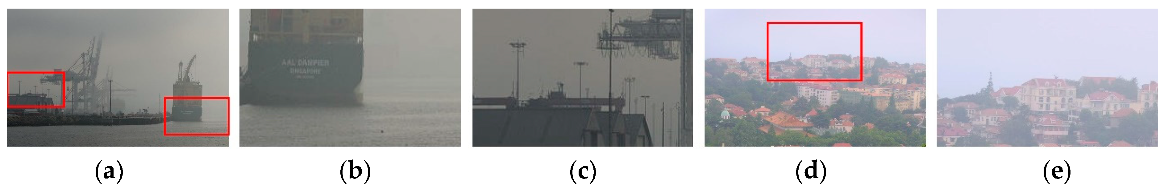
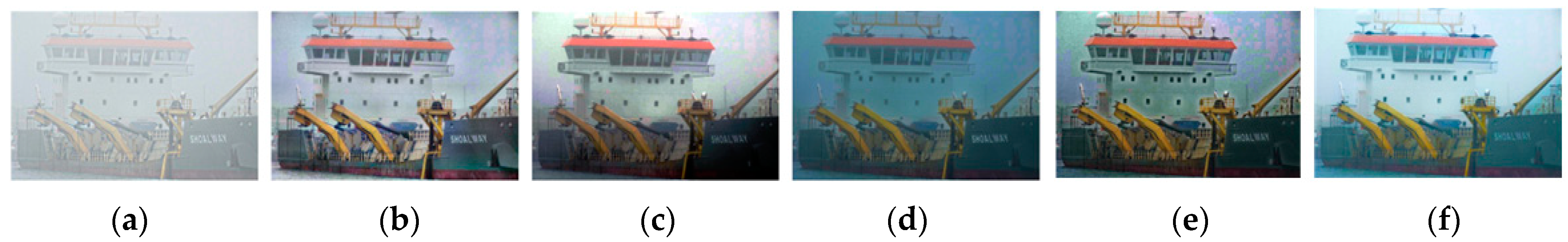
Several traditional dehazing algorithms have been proposed, including the dark channel prior method introduced by He et al. [9], the maximum-contrast method presented by Tan et al. [2], and the color-attenuation prior method proposed by Zhu et al. [17]. While existing dehazing algorithms have been effective in clearing haze in terrestrial images, they perform differently in marine settings due to distinct environmental influences. Marine images are particularly impacted by haze and atmospheric light, as well as featuring a predominant sky, leading to blurred distinctions between sky and non-sky regions. As illustrated in Figure 1, the boundaries between the sky and the ocean, and between the sky and objects, are notably indistinct in marine images, unlike in terrestrial images, where these boundaries are more clearly defined. Consequently, conventional dehazing algorithms often fail to achieve high-quality results on marine images, as they do not address the blurring of these boundaries. Figure 2 shows a comparison of dehazing outcomes for marine images, highlighting the inadequacy of traditional algorithms that overlook the unique challenges of boundary delineation in such environments. Therefore, it is essential to develop a dehazing algorithm specifically designed to effectively distinguish between sky and non-sky areas in marine images.

Figure 1.
A comparison of boundaries between maritime and terrestrial sky and non-sky areas. (b,c) are magnified portions of (a), and (e) is a magnified portion of (d). (a) is the maritime image. (b) shows the magnified boundary between the sky and maritime areas in the maritime image. (c) shows the magnified boundary between the sky and terrestrial areas in a maritime image. (d) is the terrestrial image. (e) shows the magnified boundary between the sky and terrestrial areas in the terrestrial image.

Figure 2.
Comparison of land-based defogging algorithms applied to maritime images. The input image in (a) is defogged using the algorithms of (b) Liu et al. [18], (c) T. M. Bui et al. [19], (d) He et al. [11], and (e) Wang et al. [20], as well as (f) the proposed algorithm.
Recent studies have increasingly addressed the challenges of dehazing in marine environments. For instance, Hu et al. [21] introduced a technique for light decomposition aimed at mitigating the halo effects caused by multiple scattering in marine images. Yet, this method occasionally fails to preserve structural integrity and color fidelity; this leads to a loss of detail and unnatural colors in the resulting images. T. V. Nguyen et al. [22] have developed an effective approach for illumination decomposition that maintains texture and structural integrity through stringent constraints on layer decomposition. Nonetheless, this method may introduce noise and color distortions due to oversaturation. Li et al. [23] presented a Laplacian dark channel attenuation method tailored for sea fog images, which minimizes channel discrepancies and suppresses halo effects through the use of a Laplacian function to attenuate the darkest channels. Despite its effectiveness, this method struggles with complex marine scenes and might overly adjust the image brightness, resulting in unnatural dehazing outcomes that do not accurately reflect actual conditions. Furthermore, Huang et al. [24] proposed a sea fog removal approach based on an enhanced convex optimization model that uses fewer priors than conventional methods for image restoration. However, this approach can yield unstable results when dealing with noisy or distorted input images, potentially leading to quality-impairing artifacts.
Therefore, in order to enhance the robustness of the dark channel dehazing method of He et al. [10], this study proposes a novel technique that amalgamates dark channel priors with the segmentation of boundary features in regions. This integrated approach effectively addresses the prevalent issues of atmospheric light biases in sky regions and transmittance variability in marine images.
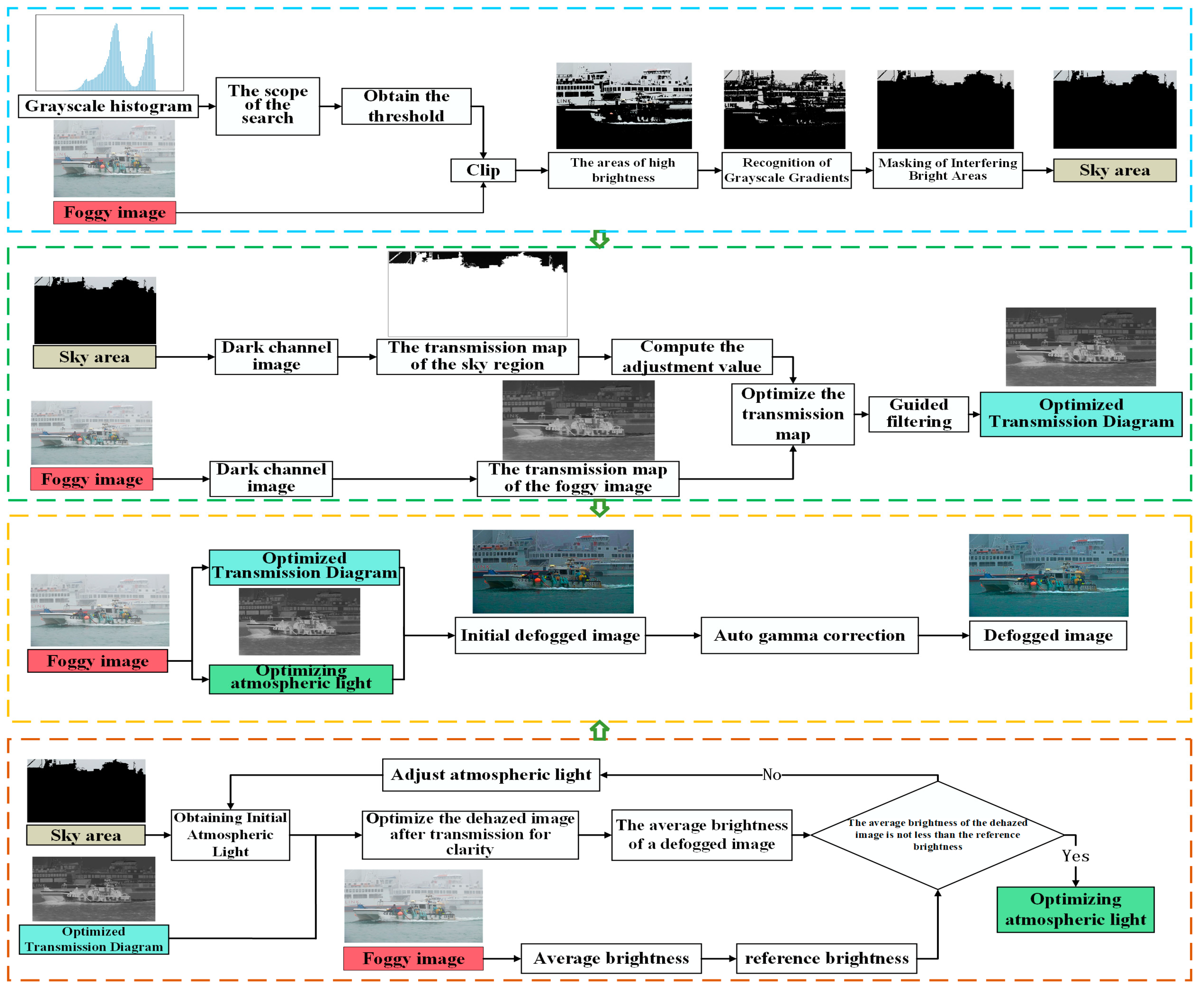
3. Proposed Methods
Figure 3 provides a detailed depiction of the dehazing algorithm process outlined in this study. Initially, initial segmentation is executed by setting thresholds based on the characteristics of grayscale value changes at regional boundaries. This process identifies areas of high brightness, including the sky, designated as . A subsequent analysis of the grayscale gradients and a comparison of region sizes allows for the refined delineation of these areas, culminating in the precise definition of the final sky region, designated as . Employing the dark channel prior theory [10], the initial transmission is extracted from I, and the atmospheric light and the transmission are estimated from . The initial transmission is optimized using and refined through guided filtering to obtain the final transmission . The algorithm iteratively adjusts to align the average brightness of the dehazed image with that of the original image, thereby accurately determining the final atmospheric light . Using and , the image is reconstructed using a physical model, and the original details are restored using an atmospheric scattering model [25], producing the preliminary dehazed image P. Finally, after applying the gamma-correction algorithm to adjust the preliminary dehazed image P, brightness balance is achieved, leading to the production of the final dehazed image J.
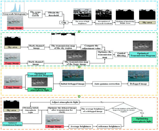
Figure 3.
A detailed depiction of the dehazing algorithm process outlined in this study.
3.1. Segmentation of the Sky Region
3.1.1. Segmentation of Boundary Features in Regions
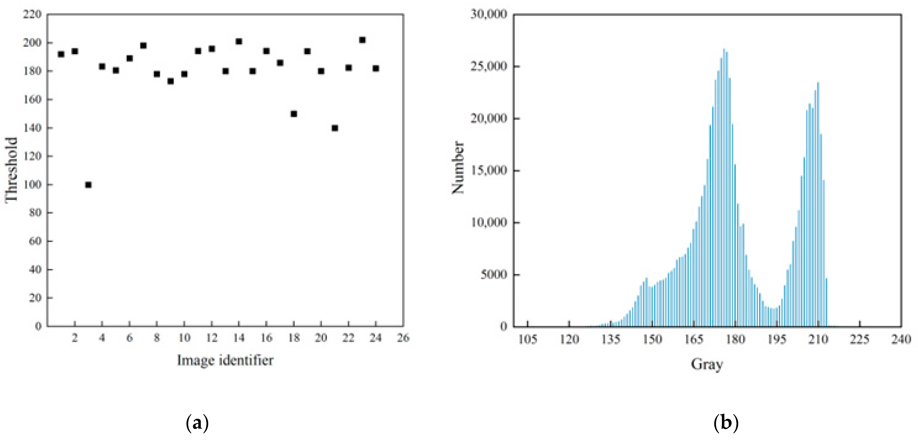
Initially, manual segmentation was performed on images across all data sets to determine each image’s optimal threshold, as detailed in Figure 4. An analysis of Figure 4a reveals that the thresholds necessary for delineating the sky in foggy maritime conditions predominantly range between grayscale values of 180–200. Upon examining the grayscale histograms for each foggy maritime image, it becomes apparent that the pixel count within the 180–200 grayscale range is minimal, especially when compared to those near the peak grayscale values. Consequently, it was ascertained that the most effective segmentation thresholds typically lie close to the peak grayscale values, where pixel counts are at their lowest, specifically within the 180–200 range. Figure 4b illustrates why the optimal threshold corresponds to this region of minimal pixel density. Typically, due to their material properties, non-sky areas, such as oceans and buildings, absorb more light than they scatter. Conversely, light scattering by aerosols and other particles predominantly determines the brightness of sky regions, making them appear brighter than non-sky areas. This results in a distinct boundary line marked by a rapid shift in grayscale values from non-sky to sky regions. Despite the continuous nature of the grayscale progression, a marked increase in values from non-sky to sky regions accompanies a notable discontinuity in pixel distribution. A distinct demarcation line emerges between these regions, characterized by consistent pixel grayscale values. The sharp transition between non-sky and sky areas contributes to a reduced pixel count at this critical threshold relative to adjacent values.
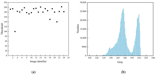
Figure 4.
Explanation of threshold selection. (a) Distribution of optimal segmentation thresholds for 25 foggy maritime images; (b) Histogram of grayscale values for the foggy maritime images.
Based on the observed phenomenon, an adaptive threshold-segmentation method was developed. This method computes the segmentation threshold by identifying grayscale values along the delineation between sky and non-sky regions, thus enabling precise distinction between these areas in images taken on foggy days. Initially, the input image I is transformed into a grayscale image using the following formula:
where R, G, and B denote the intensity values of the red, green, and blue channels, respectively. This calculation employs a weighted average based on the sensitivity of the human visual system to different colors. Then, the histogram H(g) of the grayscale image is computed, where counts(g) indicate the occurrence frequency of each grayscale value g in :
Subsequently, the indices of the top α highest values in H(g) are identified, denoted as :
Using these indices, the range for searching the optimal threshold is established, where . This range defines the interval within the histogram from to , aimed at identifying the most suitable threshold. Then, the index with the minimum count in this range is located:
Utilizing , the grayscale image is segmented to obtain the segmented image , where
Finally, using , the input image I is cropped to extract the areas of high brightness, including the sky, denoted as .
3.1.2. Recognition of Grayscale Gradients
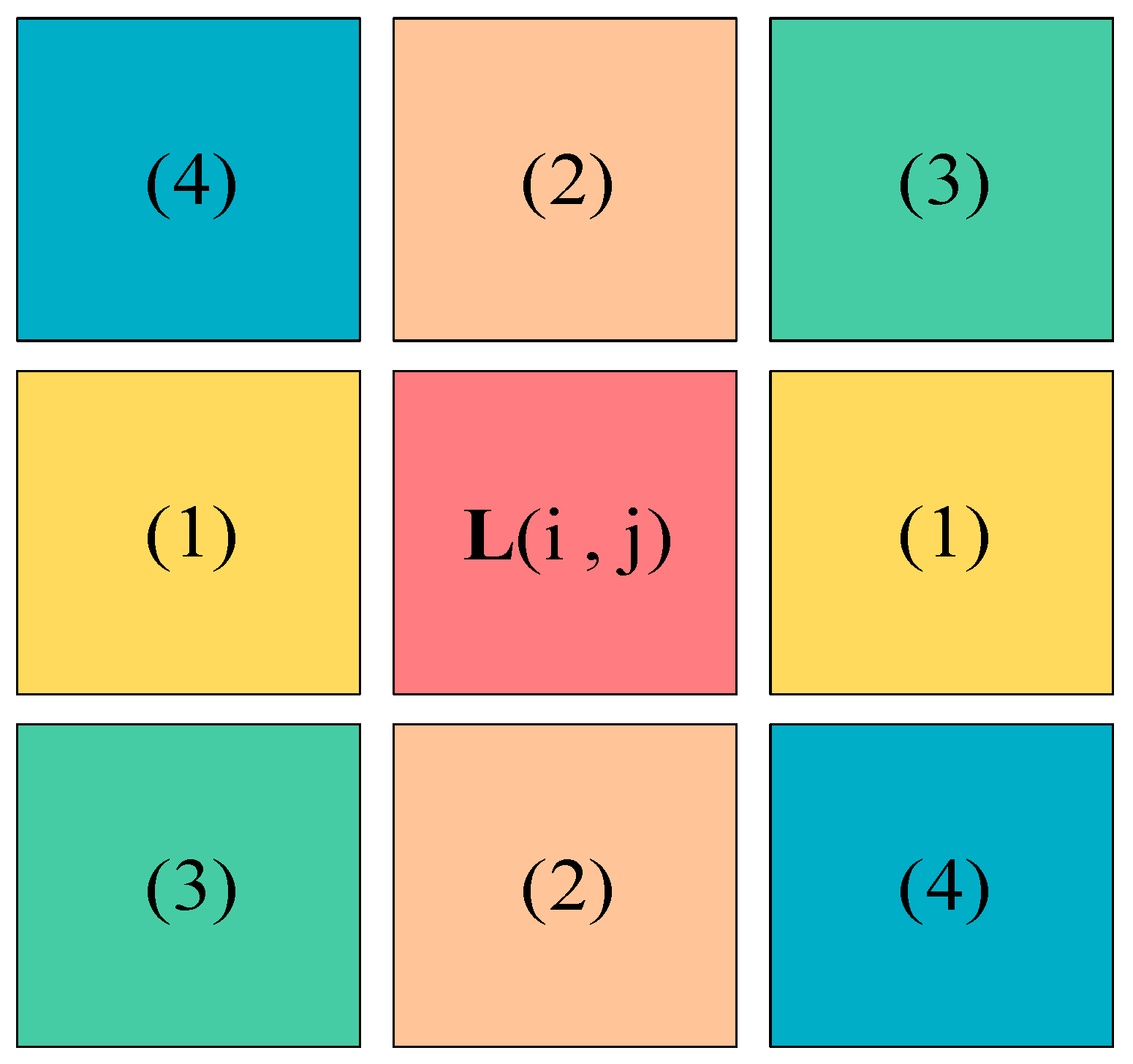
Due to the intricate nature of image environments, there may be bright targets with grayscale values closely resembling those of the sky region. Consequently, conventional threshold-segmentation methods might misclassify such bright targets as parts of the sky. Hence, this study proposes a segmentation strategy aimed at mitigating the impact of image noise. Through an extensive analysis of sky area images, it was observed that the grayscale values of the sky typically exhibit gradual changes, whereas those near the edges of bright targets undergo more pronounced variations. Leveraging this observation, each pixel of the image and its eight neighboring pixels are categorized into four groups, as illustrated in Figure 5. Subsequently, each group is scrutinized; if any pixel within a group has a grayscale value of 0, the calculation of pixel differences within that group is disregarded. Otherwise, the absolute value of the grayscale value difference between two adjacent pixels within the group is computed. Whenever the disparity in any pixel group exceeds the predetermined coefficient (denoted as β), the coordinates of the central pixel are logged and its corresponding grayscale value in the output image is set to 0, thereby completing the image-recognition process for grayscale gradients.
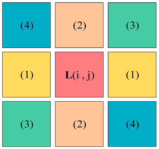
Figure 5.
L(i, j) represents the central pixel, with its surrounding eight pixels grouped into four sets labeled (1), (2), (3), and (4).
To implement the described procedure, an algorithm for the recognition of grayscale gradients is employed to identify the edges of bright targets and adjust the grayscale values of the corresponding pixels. Initially, the input sky region is transformed into a grayscale image L using Equation (1). Within this grayscale image L, the differences between each pixel L(i, j) and its neighboring pixels in four directions are computed:
These difference values, labeled as , and , are computed based on the grouping of the eight surrounding pixels, as illustrated in Figure 5, which represent the discrepancies between each group. The absolute values of these differences are utilized to detect changes in grayscale gradients within the image. If any of these difference values exceed the predetermined threshold β, the corresponding pixel is identified as part of a region undergoing significant changes.
Subsequently, for pixels meeting this criterion, the grayscale value at the corresponding position in the output image is set to 0:
3.1.3. Masking of Interfering Bright Areas
Maritime images typically display expansive horizons and large sky areas that occupy a greater proportion of the image compared to land-based images. It was identified that in images processed through the recognition of grayscale gradients, the sky area generally constitutes the largest region. Building on this insight, a novel method for image processing is introduced. This method preserves only the largest connected component as the sky, while all other components are filled with zero grayscale values, effectively identifying them as non-sky regions. The procedure is conducted as follows: initially, the output image from grayscale gradient recognition, referred to here as is processed to delineate and label each connected component in the connectivity matrix F. In this matrix, every pixel within a given connected component k is assigned an identical label . Subsequently, the area of each component is calculated, compiling these measurements into an area vector V, wherein each element denotes the area of the connected component labeled k. The method used to calculate the area of these components is outlined below:
In this approach, δ(x, y) denotes the Kronecker delta function [26], which equals 1 when x equals y and 0 otherwise. This definition indicates that represents the count of pixels labeled k, effectively measuring the area of the respective connected region. Through evaluating the elements within the vector V, the label associated with the largest connected region can be identified:
The subsequent step involves generating a new image, O, in which only the region identified by is preserved, setting the grayscale values of all other pixels to zero:
Here, O represents the processed image, which solely includes the grayscale values of the sky region. This processed image is then used as a mask to selectively extract the corresponding area from the original image I, thereby producing the final sky region image . This method effectively isolates the sky region within the image, enhancing both the accuracy and efficiency of sky detection.
3.2. Dark Channel Prior Algorithm
3.2.1. Atmospheric Scattering Model
The atmospheric scattering model introduced by McCartney is regarded as the most classical model for analyzing image degradation under foggy conditions [25]. This model comprises an incident light attenuation component that illustrates the reduction in light as it travels from the target to the observer and an atmospheric light component that considers the impact of airborne particles on the light intensity at the observer. The model is expressed by the following equation:
In this model, x represents the coordinates of pixel points in the image; J(x) is the defogged image; I(x) is the image obscured by fog; A stands for the global atmospheric light intensity; and t(x), referred to as transmission, denotes the portion of atmospheric light that reaches the camera, having been reduced by airborne particles.
3.2.2. Dark Channel Prior
He et al. [10] conducted an analysis on several clear outdoor photographs in order to establish the statistical properties of haze-free images. Their findings indicated that, in clear images devoid of the sky, at least one color channel often exhibits low pixel intensity (i.e., nearing zero). The dark channel prior theory was developed based on these findings and the atmospheric scattering model. This theory aids in transforming foggy images back to their haze-free states. The dark channel is described using the formula
In this formula, represents the dark channel image, denotes the filtering window, and c encompasses any channel among the RGB color channels in the image. To estimate atmospheric light, the method identifies the brightest points in the image; specifically, the top 0.1% of A. Knowing A and using it in conjunction with Equations (14) and (15), the transmission t(x) can be calculated as
To mitigate the image-blocking effect, the method incorporates soft matting to refine transmission. The final image representation is given by
This approach deliberately maintains a minimal level of haze in heavily fogged areas to prevent noise interference, setting to 0.1.
3.3. Optimization of Transmission
When analyzing marine fog images using the dark channel prior theory to derive transmission maps, a significant challenge was encountered: the extensive sky regions within images. These regions often yield inaccurate transmission estimates using dark channel priors. Consequently, such errors lead to underestimation of the sky’s transmission in de-fogging computations, causing excessive de-fogging and, thus, overexposure or even color anomalies in the final restored image. Overexposure not only degrades visual aesthetics but can also lead to information loss, adversely affecting image quality. Addressing these inaccuracies necessitates fine-tuning the transmission values to prevent undue restoration of sky regions during de-fogging.
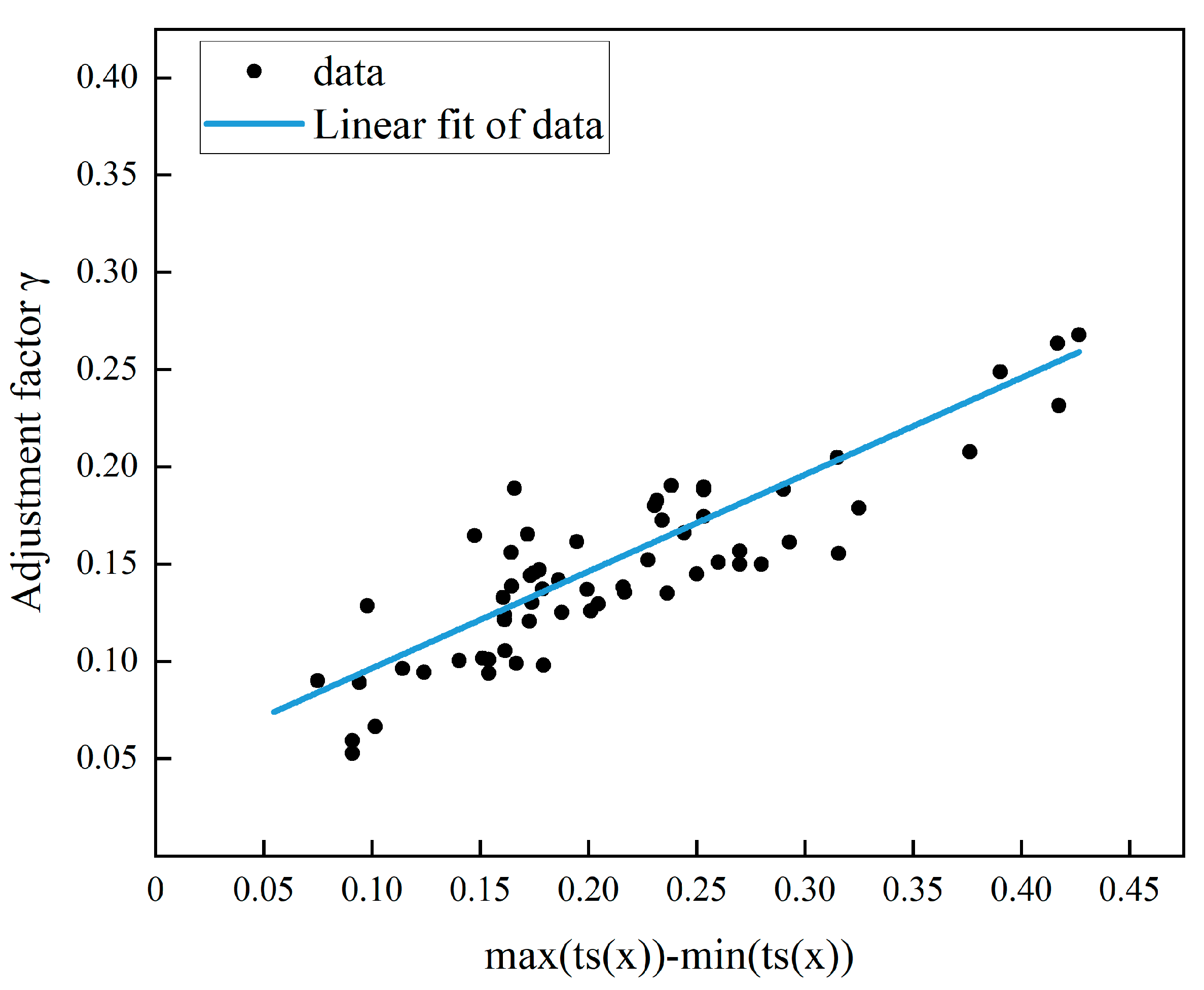
Therefore, this study proposes a method to optimize the transmission by adjusting it within specific areas, thereby enhancing the image-processing effects in sky regions. This approach employs guided filtering to eliminate noise and improve detail, preserving the edges and textural details of the image [10]. It also maintains smooth edges while effectively reducing overexposure and color distortion. Initially, transmission rates for the sky in the final image and for the input image I were calculated using dark channel priors. An adjustment factor for the sky’s transmission was then determined based on the range of . For the calculation of the appropriate adjustment factor for sky transmittance, this study recorded all manually adjusted values from the data set and conducted a linear regression using the sky transmittance ranges associated with each image, as illustrated in Figure 6. From this analysis, the following formula was established:

Figure 6.
Linear regression fitting depicting the relationship between the sky transmittance range and the adjustment factor γ.
Here, represents sky transmittance, γ is the adjustment factor, and μ is a coefficient used to optimize transmission rate set to 0.5. The coefficients μ and 0.046 were obtained through data fitting. The sky’s transmission in was subsequently adjusted, yielding an optimized transmission :
Using guidance filtering, the adjusted transmission is enhanced to derive the final transmission [10]. The grayscale image serves as the guidance image, while is the source image requiring filtration. In local regions, the guidance image and the source image exhibit a linear correlation:
Coefficients and are computed within each localized window. The objective is to optimize these coefficients to maximize the image’s overall filtering effect, expressed as
The 5 × 5 pixel window , centered on x, and a smoothing factor , set at 0.0001, facilitate this optimization. Solving for and yields
Here, and represent the mean and variance of within the window, respectively, and is the average value of within the same window. The resultant transmission is calculated as follows:
3.4. Optimization of Atmospheric Light
Upon analyzing the dehazed image Q, which is optimized for transmission, it became evident that the sky regions in sea fog images not only interfere with the transmission calculations suggested by the dark channel prior theory, but also impact the estimation of atmospheric light A. Typically, the image Q exhibits low overall brightness, appearing dimmer. This suggests that the dark channel prior theory might overestimate the value of atmospheric light A in marine settings, leading to inflated values. The atmospheric light term A quantifies the brightness of atmospheric light, where higher values of A enhance the term in the equation. As per Formula (14), to maintain constant intensity of , a steady transmission results in reduced brightness of the haze-free image , thereby decreasing the magnitude of . Accurate estimation of atmospheric light is thus crucial. Thus, the average brightness of the dehazed image Q is compared with that of the input image I, and the value of A is iteratively adjusted to align the brightness of the dehazed image more closely with that of the original image.
To enhance the accuracy of estimating the atmospheric light A, this study introduces a comparison method based on grayscale images. Initially, Equation (1) is applied to produce the grayscale images of both the input image I and the de-fogged image Q, denoted as and , respectively. The average brightnesses, and , are calculated using
Here, m and n represent the image dimensions, with i and j as the pixel coordinates. The reference grayscale value M is derived from using the global brightness compensation coefficient η:
Then, M is compared with , adjusting the atmospheric light A to compute a new de-fog image and recomputing until M no longer exceeds . The adjustment is carried out as follows:
This iterative approach fine-tunes the brightness parameter , incrementally aligning the de-fog image’s average brightness with the original image’s brightness. This process concludes once there is no further improvement in the de-fog image’s brightness, yielding the initial defogged image P.
3.5. Brightness Equalization
To mitigate the significant brightness disparity between sky and non-sky regions in the initial haze-free image , an adaptive brightness-equalization method based on gamma correction is introduced. This approach utilizes nonlinear mapping to adjust the image’s grayscale distribution, aiming to normalize the mean of all pixels close to 0.5, thereby enhancing both brightness and contrast. First, we compute the average brightness of the initial haze-free image :
Subsequently, we derive the gamma value based on :
We apply gamma correction to obtain the corrected image X:
Finally, we normalize the corrected image X to produce the haze-free image J using
This method effectively mitigates the brightness contrast between non-sky and sky regions, significantly enhancing the overall visual quality and perceptual effects of the image.
3.6. Summary of the Proposed Algorithm
The proposed method involves six steps: the segmentation of boundary features in regions, the recognition of grayscale gradients, masking interfering bright areas, transmission optimization, atmospheric light optimization, and brightness balancing. The overall aim is to improve the clarity and visibility of foggy images. First, the algorithm applies a grayscale histogram to derive a segmentation threshold appropriate for sea fog imagery, aimed at isolating the sky and other luminous regions. Subsequently, it employs a grayscale gradient and regional area parameters to delineate sky areas, effectively removing interference from other illuminated non-sky regions. In the transmission optimization stage, the algorithm calculates the sky region’s transmission to eliminate the fog effect and restore the image’s natural tones. Furthermore, atmospheric light parameters are adjusted to align the brightness of the original and processed images. Finally, brightness-balancing techniques refine the image quality, ensuring that the de-fogged image maintains consistency with the original foggy image in terms of color and brightness. For reference, the algorithm pseudocode is provided in Algorithm 1.
| Algorithm 1: Detailed Defogging Algorithm Process |
| Input: Foggy image I, parameters α, β, γ, μ, η, θ Output: Defogged image J 1. Segmentation of Boundary Features in Regions Convert the input image I to a grayscale image denoted as Calculate the histogram of the grayscale image, represented by H(g) Identify the indices of the top maximum values in the histogram as Define the search interval Locate the index with the minimum histogram count within as Segment the initial sky region where , and crop to obtain the areas of high brightness . 2. Recognition of Grayscale Gradients For each pixel (i, j) and its eight neighboring pixels, compute the grayscale difference across four directions . If any difference exceeds the threshold σ: set the grayscale value of that pixel to 0 in the output image 3. Masking of Interfering Bright Areas Label the connected areas in to obtain the connected area matrix F Compute the area of each area as Identify the largest area by its label Generate a new image O that retains only the area labeled 4. Optimization of Transmission Calculate the transmission rates for the sky area in the final image and the input image I as and respectively. Adjust the sky area’s transmission rate Update the transmission rate for the sky part in to Guided filtering optimizes to 5. Optimization of Atmospheric Light Compute the grayscale images and the average brightness of the input and defogged images, and , as and respectively. Calculate the reference grayscale value Adjust the atmospheric light A 6. Brightness Equalization Obtain the average brightness value from the initial defogged , and calculate the gamma value as follows: Apply gamma correction to obtain the corrected image X: Normalize the corrected image X to generate the final haze-free image J: |
4. Results
Data available through Internet searches and self-collection were obtained, and an image library containing more than 100 foggy images monitored at sea was constructed. We compared our method with the algorithms previously proposed by He et al. [11], T. V. Nguyen et al. [21], Hu et al. [20], Kaplan N.H. [26], and Liu et al. [27]. Through executing online open-source codes, we conducted subjective and objective evaluations of their image processing results against our results. In the experiments, the parameter α in Formula (3) and the parameter β in Formula (10) were set to 25 and 2.5, respectively, while the parameter μ in Formula (18) and the parameter η in Formula (24) were fixed at 0.5 and 0.45, respectively. In a large number of experiments, the above parameter settings produced good overall subjective visual effects and performed well in terms of objective quantitative evaluation.
4.1. Subjective Analysis
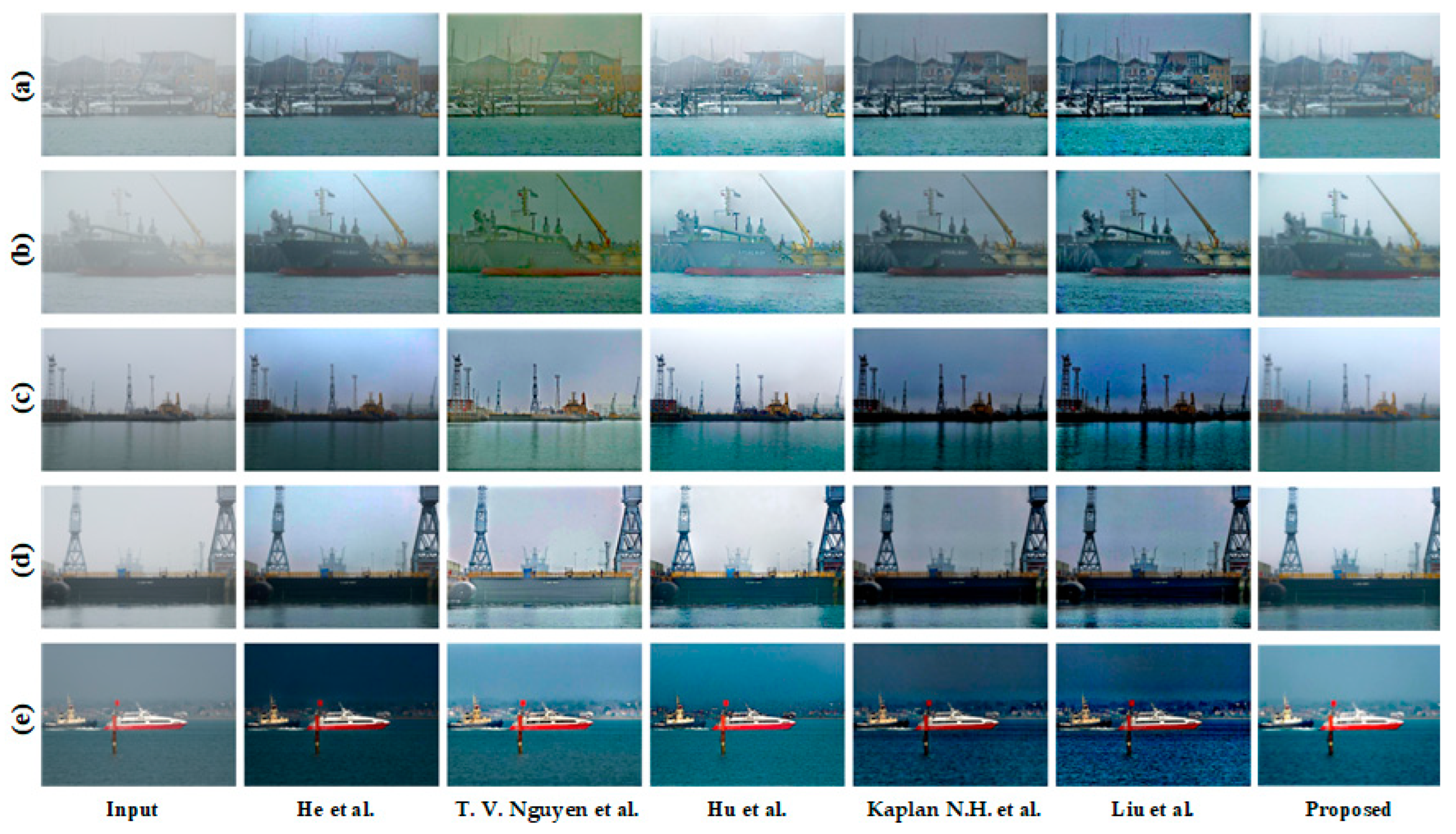
We compared the haze-removal results, as shown in Figure 7. The algorithm proposed by He et al. [11] (second column) caused the non-sky areas of the dehazed image to become darker overall, resulting in lower image brightness. These problems arise due to the foggy images obtained from maritime surveillance images differing from general foggy images. The images contain a large number of clear areas, such as the sky, which are usually mixed with foggy areas. The algorithm proposed by T. V. Nguyen et al. [22] (third column) includes an innovative illumination-decomposition method to remove halos caused by complex scattering in ocean images. However, this technology sometimes has difficulty in maintaining the consistency of the image structure and color when removing haze. For example, as shown in Figure 7a,c, due to the relatively heavy haze content of the input image, during the process of enhancing the image color, it overcompensates for certain colors and fails to properly balance colors, resulting in color distortion. At the same time, the algorithm proposed by Hu et al. [21] (fourth column) had good effects in terms of the clarity of the picture and the processing of the sky part, but the dehazing effect was not good (see, e.g., Figure 7a,b): as the fog concentration in different parts of the picture is not the same, the global unified dehazing method will lead to incomplete dehazing in some places, which may lead to sharpening or even color deviation. Regarding the algorithms of Kaplan N.H. [27] (fifth column) and Liu et al. [18] (sixth column; see, e.g., Figure 7c,e), although a notable contrast enhancement in the dehazed image indicates improvement, noise may occur during processing, which results in color distortion due to oversaturation, especially in the reflective parts of the sky and water. The processed image appears too dark, especially in dark areas in which some detail may have been lost. On the contrary, as shown in Figure 7d, our proposed algorithm had a significant effect on image dehazing. The overall image after dehazing has balanced color, contrast, and brightness, as well as minimal noise. As such, the clarity and visual effect of the image are guaranteed.

Figure 7.
Qualitative comparison of different methods for defogging maritime images. The foggy input images (first column) were restored using the algorithms of He et al. [11] (second column), T. V. Nguyen et al. [22] (third column), Hu et al. [21] (fourth column), Kaplan N.H. et al. [27] (fifth column), and Liu et al. [18] (sixth column), as well as the proposed algorithm (seventh column). Each row, labeled from (a–e), corresponds to distinct maritime scenes, providing a side-by-side comparison of the effectiveness of each algorithm under varying fog conditions.
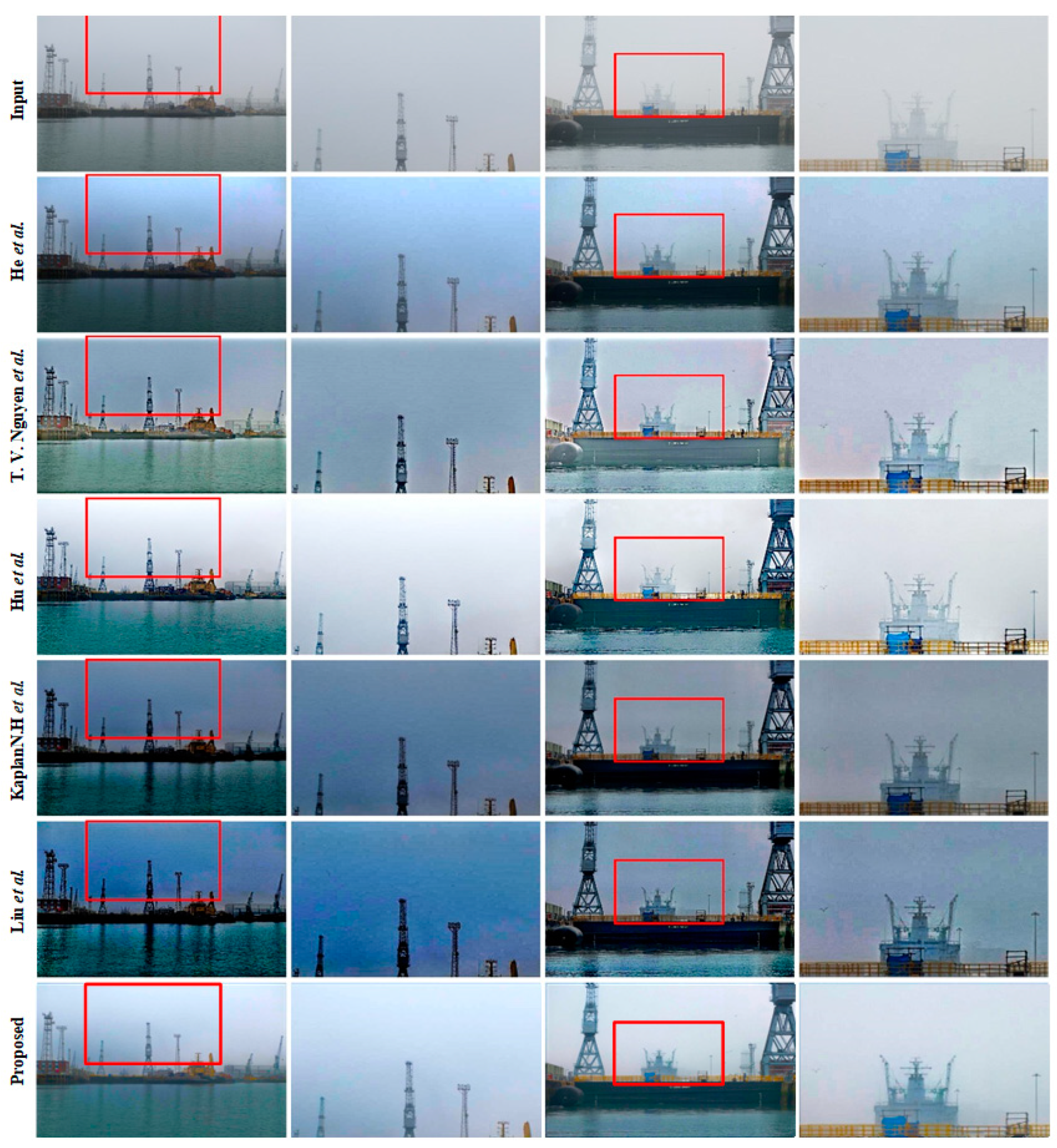
Figure 8 shows and compares the details of dehazed local images. He et al.’s algorithm [11] (second row) darkened the image. The algorithm proposed by T. V. Nguyen et al. [22] (third row) had a better texture quality than the algorithm of He et al. [11] but failed to effectively balance the overall color, resulting in color distortion and artifacts at the edges of objects, thus creating a halo effect. With the algorithm created by Hu et al. [21] (fourth row), dehazing unevenly in the sky area led to a sharpening of local areas after dehazing. The algorithms created by Kaplan N.H. [27] (fifth column) and Liu et al. [18] (sixth column) had better contrast in the dehazed local image, but some details were lost due to the generation of noise. In contrast, the proposed algorithm (seventh row) retained the local details of the image and not only effectively removed fog but also enhanced the contrast and suppressed the generation of noise. As our algorithm takes into account the sea and sky during the dehazing process, the overall resulting image has better smoothness.
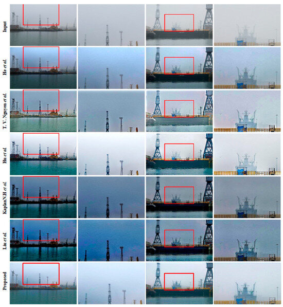
Figure 8.
Comparison of demisting outcomes for the misty maritime images and their amplified segments. The second and fourth columns correspondingly exhibit enlarged portions of the crimson rectangles in the initial and subsequent columns.
4.2. Objective Evaluation
As the human eye tends to lose some details when observing pictures, the subjective evaluation of images may be biased. In terms of objective evaluation, 11 objective quality-evaluation methods were utilized to compare the existing algorithms with the algorithm proposed in this article: the Structural Similarity Performance Index (SSIM) [28], Peak Signal-to-Noise Ratio (PSNR), Natural Image Quality Evaluator (NIQE) [29], Mean Square Error (MSE), CIEDE2000 (CIEDE) [30], rate of new visible edges (e) [31], number of saturated pixels after restoration (σ) [31], restoration quality (r) [31], Contrast Enhancement Index (CII), Equivalent Number of Views (ENL), Lightness Order Error (LOE), and No-Reference Structural Sharpness Score (NRSS). The results are presented in Table 1. In this way, we quantitatively evaluated the average performance of all algorithms. In accordance with the experimental setup outlined in this study, the foggy images employed were obtained from real scenes rather than artificially generated without fog through algorithms. Therefore, the present study utilized the original foggy image as a benchmark to evaluate PSNR and SSIM values for images processed by the defogging algorithm, thereby assessing the impact of each algorithm on image quality. Extremely low PSNR and SSIM scores indicate that the defogging algorithm may severely degrade the image quality, increase noise levels, and render the image unusable. Conversely, higher PSNR and SSIM scores signify minimal image damage and enhance the reliability of other measurement indicators. When these metrics are considered together, they provide a more accurate and comprehensive evaluation of the algorithm’s performance. To measure the performance of each indicator, we adopted the following criteria to clearly express the relative advantages of the data: the table highlights the best results in bold, while the top three results are underlined. Given the data presented in Table 1, the algorithm proposed in this article performed well in terms of various performance indicators on different images (usually ranking in the top three) and achieved the best results among all algorithms in multiple indicators. Based on the performance of PSNR and SSIM, Hu et al.’s algorithm and the current algorithm exhibit minimal image degradation and stable defogging effects. Conversely, other algorithms generate significant noise in some images and demonstrate inconsistent results. When combined with other evaluation metrics, it is evident that existing algorithms fail to consistently achieve superior performance across various image parameters. For example, the algorithm proposed by He et al. performed poorly in the e, σ, and ENL indicators, demonstrating the problems of incomplete dehazing and low image smoothness. In contrast, the algorithm proposed by T. V. Nguyen et al. scored lower in the CIEDE and LOE metrics, exposing flaws related to color distortion and a lack of naturalness in the image. For the algorithm created by Hu et al., its low scores in the CII and NRSS metrics reflect the insufficient contrast and sharpness of the image. However, the algorithms of Kaplan N.H. and Liu et al. scored low in most evaluation indicators, especially having the worst performance in NIQE, PSNR, and LOE, indicating that these algorithms have weak noise-processing abilities.

Table 1.
A quantitative assessment of quality metrics for mist removal: SSIM [28], PSNR, MSE, NIQE [29], CIEDE [30], e [31], σ [31], r [31], CII, LOE, ENL, and NRSS. For each criterion, the bold value denotes the optimal outcome. The best results for each metric are highlighted in bold, while the top three results are underlined to clearly display relative performance.
4.3. The Impact of Image Segmentation on Dehazing
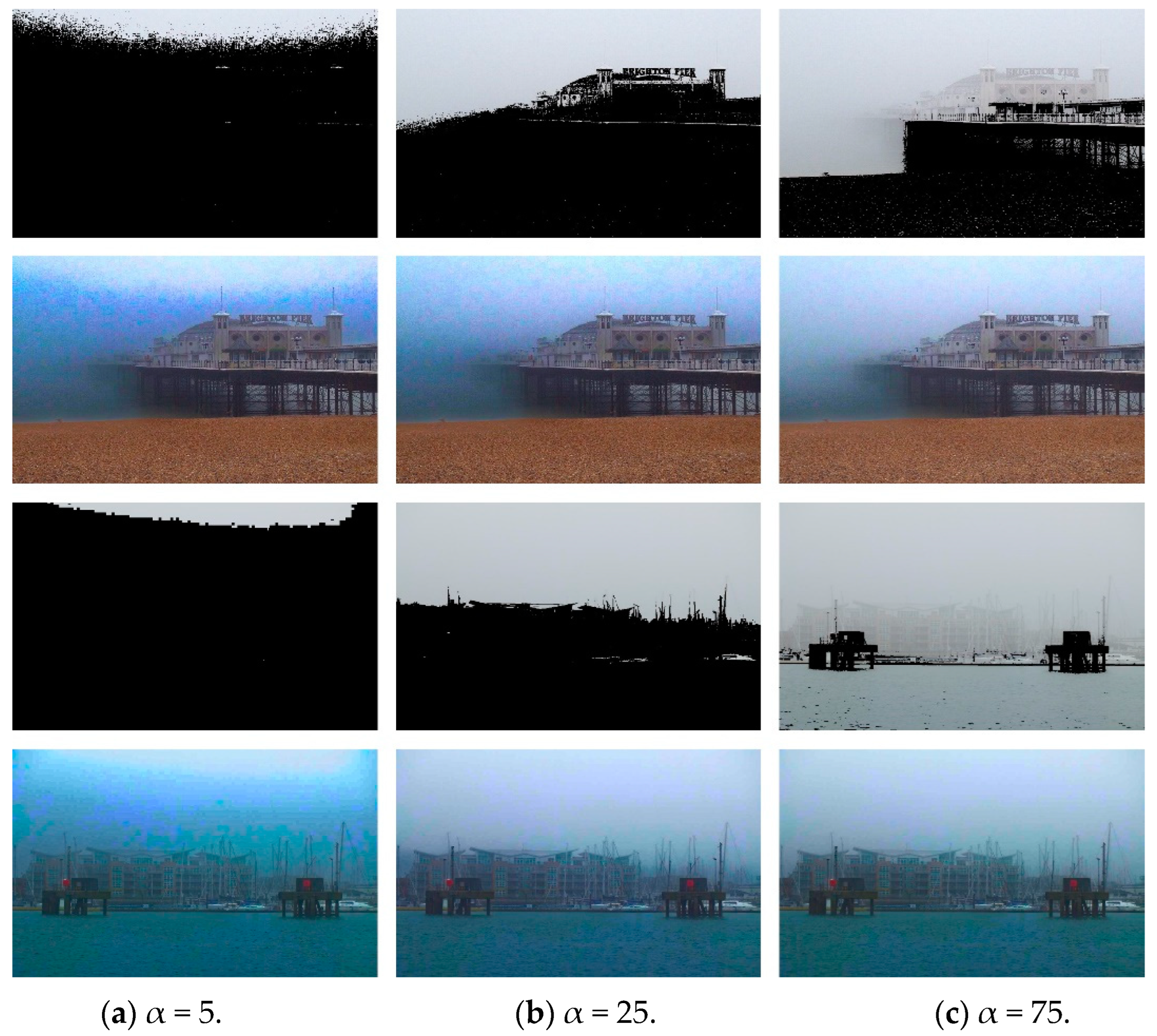
In Section 3.1, we introduced two key parameters for image segmentation: parameter α in Equation (3) and parameter β in Equation (10). The parameter α in Equation (3) is used to control the threshold-selection range. As shown in Figure 9, the value of α directly affects the size of the threshold. An α value that is too low will make the threshold too large, resulting in insufficient selection of the sky area and an inability to completely segment the sky area. As a result, areas of the sky that are not completely segmented will be over-processed during the dehazing process, causing problems such as overexposure, color spots, and color casts. On the contrary, if the α value is too high, both sky and non-sky areas may be selected, which will not achieve the purpose of effective segmentation. If the non-sky area is mistakenly classified as a sky area, it will lead to problems such as reduced image quality in this area and a poor dehazing effect.
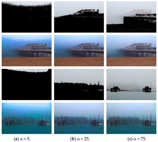
Figure 9.
The defogging outcomes of the proposed algorithm for varying α weights: (a) α = 5; (b) α = 25; (c) α = 75. The first and third rows display the outcomes of threshold-based segmentation, while the second and third columns display the corresponding defogged images.
Parameter β in Equation (10) is used to control the sensitivity of grayscale gradient recognition. Setting a β value that is too low may cause the recognition of grayscale gradients to be too sensitive, thus generating a lot of noise in the sky area. As depicted in Figure 10, when there is extensive noise in the sky, erroneously connected areas may be formed, causing problems when filling these areas and seriously affecting the segmentation effect. This results in an uneven image-dehazing effect, an overexposed noise area, and possible color distortion. Meanwhile, a high β value may cause insufficient sensitivity in the recognition of grayscale gradients such that some edges are not recognized. Therefore, when connected areas are filled, these edges are not filled, resulting in a sky mixed with non-sky areas that are still affected by fog. Therefore, it is crucial to accurately adjust the parameters α and β to ensure effective image segmentation.
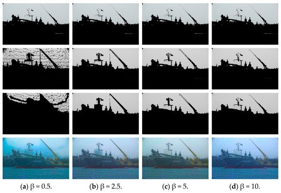
Figure 10.
The defogging outcomes of the proposed algorithm for varying β weights: (a) β = 0.5; (b) β = 2.5; (c) β = 5; (d) β = 10. The first row displays the results of threshold segmentation, the second row shows the recognition of grayscale gradient outcomes, the third row illustrates connected region filling, and the fourth row presents the defogged images.
4.4. The Impact of Other Parameters on Dehazing
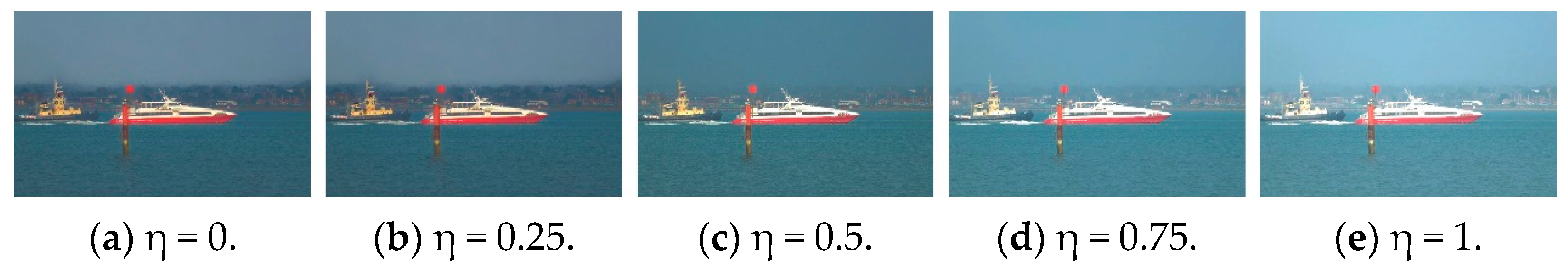
In Section 3.4 and Section 3.5 and II-E, the parameters used to optimize transmittance and brightness compensation were explored, namely, μ in Equation (18) and η in Equation (27), which greatly influence the defogging effect. As illustrated in Figure 11, μ in Equation (2) mainly controls the transmittance of the sky area; therefore, the set value of μ affects the degree of haze removal in the sky area. A lower μ can reduce the transmittance of the sky, thereby clearing more fog and enhancing the visual clarity of the area. However, if μ is too low, excessive dehazing, overexposure of the sky area, and/or image distortion may occur. As μ increases, the naturalness of the image increases; however, if the μ value is too high, the defogging effect will be reduced. In Equation (28), the functions of η are reflected in the brightness adjustment. As shown in Figure 12, η mainly determines the global brightness of the image, where a lower η will decrease the overall luminance of the image after dehazing. As the η value increases, the overall brightness of the image gradually increases, which is more in line with natural observation conditions. Therefore, in order to ensure the best visual quality, we fixed the values of μ and η at 0.5 and 0.45, respectively, in the algorithm. These parameter settings are designed to balance the dehazing effect and naturalness of the image to achieve an ideal visual experience.
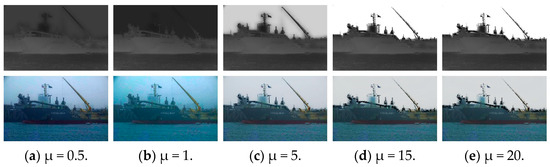
Figure 11.
The defogging outcomes of the proposed algorithm for varying μ weights: (a) μ = 0.5; (b) μ = 1; (c) μ = 5; (d) μ = 15; (e) μ = 20. The transmission maps are presented in the first row, and the corresponding defogged images are displayed in the second row.
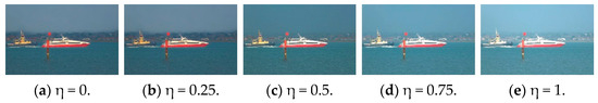
Figure 12.
The defogging outcomes of the proposed algorithm for varying η weights: (a) η = 0; (b) η = 0.5; (c) η = 0.5; (d) η = 0.75; (e) η = 1.
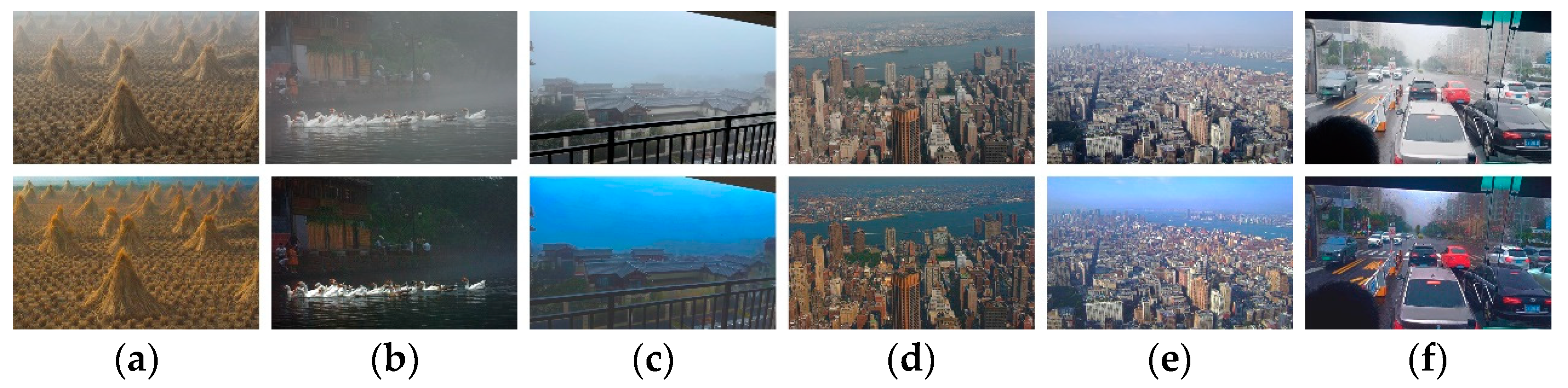
4.5. Application to Land Image Defogging
We analyzed the differences between sea fog and land fog by applying the proposed algorithm to land images. Although this method is mainly used for dehazing foggy ocean images, we found that in normal foggy images, the influence of the sky area is also significant. As the dark channel prior theory is not fully applicable to certain sky parts in foggy land images, especially under dense fog conditions, traditional defogging techniques often result in overexposed images or poor dehazing effects. By segmenting the sky area and balancing the brightness, our method is also suitable for processing normal foggy images, and its performance is not affected by the marine environment. To demonstrate the processing effect of the algorithm introduced in this paper on foggy images, Figure 13 presents the results after applying image-segmentation, optimized transmittance and atmospheric light, and brightness-equalization methods. It can be seen that the algorithm not only performs well in processing ocean fog images but also has good adaptability to land fog images.

Figure 13.
Defogging outcomes of land fog images, presenting input images in the top row and corresponding defogged results in the bottom row. (a,b) Land images without sky regions and (c–f) land images with sky regions.
4.6. Efficiency Analysis
The experiments were performed on a personal computer configured with 16 GB of RAM and a 2.6 GHz CPU. In the experiment, the image sizes were adjusted to 800 × 600 pixels, 1000 × 800 pixels, 15,000 × 1000 pixels, and 25,000 × 1200 pixels, respectively. Table 2 compares the time efficiency of various defogging techniques. Given that this study primarily aimed to enhance the dehazing quality of foggy ocean images, the speed of the proposed method is not exceptionally remarkable. In the proposed method, the recognition of grayscale gradients and the adjustment of the atmospheric light A are the main time-consuming steps. Recognizing grayscale gradients requires a calculation for each pixel in the image, and the process of adjusting the atmospheric light A requires about 10 to 15 iterations. This study’s algorithm, which builds on the method proposed by He et al., aims to enhance the quality of dehazed images. As a result, it operates at a slower speed compared to the original algorithm. The algorithm proposed in this article was twice as fast as the dehazing methods based on illumination decomposition introduced by Hu et al. and T. V. Nguyen et al. Although our speed was slightly inferior to that of the fast dehazing methods based on CEEF by Liu et al. and Kaplan N.H., the proposed method provides a far better image dehazing quality. We are working hard to further simplify the processes of grayscale gradient recognition, transmittance t(x), and atmospheric light A optimization in order to establish a dehazing model with improved efficiency and practicality compared to the proposed dehazing method.
Table 2.
Average computation times (in seconds) of the algorithms introduced by He et al. [11], T. V. Nguyen et al. [22], Hu et al. [21], Kaplan N.H. [27], and Liu et al. [18], as well as the proposed algorithm.
5. Conclusions
This study proposes an adaptive sky region segmentation method coupled with a dark channel prior technique for clarifying dehazed maritime images. Initially, a threshold suitable for sea fog characteristics is derived through a grayscale histogram approach to delineate bright zones such as the sky. Subsequently, by employing grayscale gradients and area parameters, the sky region is distinguished, adaptively eliminating interference from other bright, non-sky areas and achieving precise segmentation. Furthermore, a transmittance optimization algorithm, augmented by guided filtering techniques, adjusts the transmittance to restore the original image’s details. The atmospheric light intensity is then methodically adjusted using an optimization algorithm, ensuring the dehazed image maintains a brightness level comparable to the original. Moreover, applying the gamma-correction algorithm enhances defogged images by reducing brightness discrepancies between sky and non-sky regions, thereby improving visual clarity. Through comparative qualitative and quantitative analyses, the method presented in this study shows significant superiority in dehazing quality compared to existing algorithms. Concurrently, it reduces the risk of maritime transportation accidents. In the future, this technology is poised to expand into urban transportation, military equipment, meteorological observations, and other sectors, offering promising market prospects.
Author Contributions
Conceptualization, K.H., Q.Z. and J.W.; methodology, K.H., J.H. and Q.Y.; software, K.H. and Q.Z.; validation, J.H. and Q.Y.; writing—original draft preparation, K.H., Q.Z. and J.W.; writing—review and editing, J.H. and Q.Y.; visualization, K.H., Q.Z. and J.W.; project administration, J.H. and Q.Y.; funding acquisition, J.H. and Q.Y. All authors have read and agreed to the published version of the manuscript.
Funding
This research was supported by the Key Research and Development Projects in Hainan Province, China, in 2024 (No. ZDYF2024SHFZ089). The project leader is Jianqing Huang.
Institutional Review Board Statement
Not applicable.
Informed Consent Statement
Written informed consent has been obtained from the patient to publish this paper.
Data Availability Statement
The data presented in this study are available in defogging-for-sea-fog-images-TIP2020. These data were derived from the following resources available in the public domain: https://github.com/yeyekurong/defogging-for-sea-fog-images-TIP2020, accessed on 12 July 2024.
Acknowledgments
This study was funded by the Key Research and Development Initiatives in Hainan Province, China, in 2024, with the project identifier ZDYF2024SHFZ089. All support is gratefully acknowledged.
Conflicts of Interest
The authors declare no conflicts of interest.
References
- Narasimhan, S.G.; Nayar, S.K. Vision and the Atmosphere. Int. J. Comput. Vis. 2002, 48, 233–254. [Google Scholar] [CrossRef]
- Tan, R.T. Visibility in bad weather from a single image. In Proceedings of the 2008 IEEE Conference on Computer Vision and Pattern Recognition, Anchorage, AK, USA, 23–28 June 2008; pp. 1–8. [Google Scholar] [CrossRef]
- Li, B.; Ren, W.; Fu, D.; Tao, D.; Feng, D.; Zeng, W.; Wang, Z. Benchmarking SingleImage Dehazing and Beyond. IEEE Trans. Image Process. 2019, 28, 492–505. [Google Scholar] [CrossRef] [PubMed]
- Xu, Y.; Wen, J.; Fei, L.; Zhang, Z. Review of Video and Image Defogging Algorithms and Related Studies on Image Restoration and Enhancement. IEEE Access 2016, 4, 165–188. [Google Scholar] [CrossRef]
- Sabir, A.; Khurshid, K.; Salman, A. Segmentationbased image defogging using modified dark channel prior. J. Image Video Process. 2020, 2020, 6. [Google Scholar] [CrossRef]
- Pizer, S.M.; Amburn, E.P.; Austin, J.D.; Cromartie, R.; Geselowitz, A.; Greer, T.; ter Haar Romeny, B.; Zimmerman, J.B.; Zuiderveld, K. Adaptive histogram equalization and its variations. Comput. Vis. Graph. Image Process. 1987, 39, 355–368. [Google Scholar] [CrossRef]
- Fan, T.; Li, C.; Ma, X.; Chen, Z.; Zhang, X.; Chen, L. An improved single image defogging method based on Retinex. In Proceedings of the 2017 2nd International Conference on Image, Vision and Computing (ICIVC), Chengdu, China, 2–4 June 2017; pp. 410–413. [Google Scholar] [CrossRef]
- Deng, G.; Galetto, F.; Alnasrawi, M.; Waheed, W. A Guided Edge-Aware Smoothing-Sharpening Filter Based on Patch Interpolation Model and Generalized Gamma Distribution. IEEE Open J. Signal Process. 2021, 2, 119–135. [Google Scholar] [CrossRef]
- He, K.; Sun, J.; Tang, X. Single Image Haze Removal Using Dark Channel Prior. IEEE Trans. Pattern Anal. Mach. Intell. 2011, 33, 2341–2353. [Google Scholar] [CrossRef] [PubMed]
- He, K.; Sun, J.; Tang, X. Guided Image Filtering. In Computer Vision—ECCV 2010. ECCV 2010; Lecture Notes in Computer Science; Daniilidis, K., Maragos, P., Paragios, N., Eds.; Springer: Berlin/Heidelberg, Germany, 2010; Volume 6311. [Google Scholar] [CrossRef]
- He, K.; Sun, J. Fast Guided Filter. arXiv 2015, arXiv:1505.00996. [Google Scholar]
- Lee, S.; Yun, S.; Nam, J.-H.; Won, C.S.; Jung, S.-W. A review on dark channel prior based image dehazing algorithms. J. Image Video Process. 2016, 2016, 4. [Google Scholar] [CrossRef]
- Tarel, J.-P.; Hautiere, N. Fast visibility restoration from a single color or gray level image. In Proceedings of the 2009 IEEE 12th International Conference on Computer Vision, Kyoto, Japan, 29 September–2 October 2009. [Google Scholar]
- Cai, B.; Xu, X.; Jia, K.; Qing, C.; Tao, D. DehazeNet: An End-to-End System for Single Image Haze Removal. IEEE Trans. Image Process. 2016, 25, 5187–5198. [Google Scholar] [CrossRef]
- Ren, W.; Liu, S.; Zhang, H.; Pan, J.; Cao, X.; Yang, M.-H. Single image dehazing via multi-scale convolutional neural networks. In Proceedings of the Computer Vision–ECCV 2016: 14th European Conference, Amsterdam, The Netherlands, 11–14 October 2016; Proceedings, Part II 14, 2016. pp. 154–169. [Google Scholar]
- Zhang, H.; Patel, V.M. Densely Connected Pyramid Dehazing Network. In Proceedings of the 2018 IEEE/CVF Conference on Computer Vision and Pattern Recognition (CVPR), Salt Lake City, UT, USA, 18–23 June 2018; pp. 3194–3203. [Google Scholar] [CrossRef]
- Zhu, Q.; Mai, J.; Shao, L. A Fast Single Image Haze Removal Algorithm Using Color Attenuation Prior. IEEE Trans. Image Process. 2015, 24, 3522–3533. [Google Scholar] [CrossRef]
- Liu, X.; Li, H.; Zhu, C. Joint Contrast Enhancement and Exposure Fusion for Real-World Image Dehazing. IEEE Trans. Multimed. 2022, 24, 3934–3946. [Google Scholar] [CrossRef]
- Bui, T.M.; Kim, W. Single Image Dehazing Using Color Ellipsoid Prior. IEEE Trans. Image Process. 2018, 27, 999–1009. [Google Scholar] [CrossRef]
- Wang, X.-M.; Huang, C.; Li, Q.-B.; Liu, J.-G. Improved Multiscale Retinex Image Enhancement Algorithm. J. Comput. Appl. 2010, 30, 2091–2093. [Google Scholar]
- Hu, H.-M.; Guo, Q.; Zheng, J.; Wang, H.; Li, B. Single Image Defogging Based on Illumination Decomposition for Visual Maritime Surveillance. IEEE Trans. Image Process. 2019, 28, 2882–2897. [Google Scholar] [CrossRef] [PubMed]
- Van Nguyen, T.; Mai, T.T.N.; Lee, C. Single Maritime Image Defogging Based on Illumination Decomposition Using Texture and Structure Priors. IEEE Access 2021, 9, 34590–34603. [Google Scholar] [CrossRef]
- Li, Z.-X.; Wang, Y.-L.; Peng, C.; Peng, Y. Laplace dark channel attenuation-based single image defogging in ocean scenes. Multimedia Tools Appl. 2023, 82, 21535–21559. [Google Scholar] [CrossRef]
- Huang, H.; Li, Z.; Niu, M.; Miah, S.; Gao, T.; Wang, H. A Sea Fog Image Defogging Method Based on the Improved Convex Optimization Model. J. Mar. Sci. Eng. 2023, 11, 1775. [Google Scholar] [CrossRef]
- McCartney, E.J.; Hall, F.F. Optics of the Atmosphere: Scattering by Molecules and Particles. Phys. Today 1977, 30, 76–77. [Google Scholar] [CrossRef]
- Kronecker, L. Grundzüge einer arithmetischen Theorie der algebraischen Grössen. J. Reine Angew. Math. 1853, 44, 93–122. [Google Scholar]
- Kaplan, N.H. Real-world image dehazing with improved joint enhancement and exposure fusion. J. Vis. Commun. Image Represent. 2023, 90, 103720. [Google Scholar] [CrossRef]
- Wang, Z.; Bovik, A.C.; Sheikh, H.R.; Simoncelli, E.P. Image quality assessment: From error visibility to structural similarity. IEEE Trans. Image Process. 2004, 13, 600–612. [Google Scholar] [CrossRef] [PubMed]
- Mittal, A.; Soundararajan, R.; Bovik, A.C. Making a “completely blind” image quality analyzer. IEEE Signal Process. Lett. 2012, 20, 209–212. [Google Scholar] [CrossRef]
- Sharma, G.; Wu, W.; Dalal, E.N. The CIEDE2000 color-difference formula: Implementation notes, supplementary test data, and mathematical observations. Color Res. Appl. 2005, 30, 21–30. [Google Scholar] [CrossRef]
- Hautiere, N.; Tarel, J.P.; Aubert, D.; Dumont, E. Blind contrastenhancement assessment by gradient ratioing at visible edges. Image Anal. Stereol. 2011, 27, 87–95. [Google Scholar] [CrossRef]


Disclaimer/Publisher’s Note: The statements, opinions and data contained in all publications are solely those of the individual author(s) and contributor(s) and not of MDPI and/or the editor(s). MDPI and/or the editor(s) disclaim responsibility for any injury to people or property resulting from any ideas, methods, instructions or products referred to in the content. |
© 2024 by the authors. Licensee MDPI, Basel, Switzerland. This article is an open access article distributed under the terms and conditions of the Creative Commons Attribution (CC BY) license (https://creativecommons.org/licenses/by/4.0/).