Abstract
With the wide application of Underwater Wireless Sensor Networks (UWSNs) in various fields, more and more attention has been paid to deploying and adjusting network nodes. A UWSN is composed of nodes with limited mobility. Drift movement leads to the network structure’s destruction, communication performance decline, and node life-shortening. Therefore, a Node Adjustment Scheme based on Motion Prediction (NAS-MP) is proposed, which integrates the layered model of the ocean current’s uneven depth, the layered ocean current prediction model based on convolutional neural network (CNN)–transformer, the node trajectory prediction model, and the periodic depth adjustment model based on the Seagull Optimization Algorithm (SOA), to improve the network coverage and connectivity. Firstly, the error threshold of the current velocity and direction in the layer was introduced to divide the depth levels, and the regional current data model was constructed according to the measured data. Secondly, the CNN–transformer hybrid network was used to predict stratified ocean currents. Then, the prediction data of layered ocean currents was applied to the nodes’ drift model, and the nodes’ motion trajectory prediction was obtained. Finally, based on the trajectory prediction of nodes, the SOA obtained the optimal depth of nodes to optimize the coverage and connectivity of the UWSN. Experimental simulation results show that the performance of the proposed scheme is superior.
1. Introduction
With the increasing demand for ocean observation and exploration, UWSNs have attracted much attention recently. UWSNs are widely used in marine environmental monitoring, ecological protection, sonar navigation, resource utilization, and military surveillance [1].
In UWSNs, the proper deployment of nodes is very important to the communication performance of the whole network, including network coverage, connectivity, energy consumption, and lifespan. Furthermore, the node deployment can be divided into static, restricted movement, and completely free movement. Static deployment means that nodes do not move and are fixed in predefined positions. The movement range of those restricted mobile nodes is small. A fully mobile node means that all ordinary nodes move. Due to the water flow, underwater nodes will move. Compared with fixed deployment, the mobile deployment of ordinary nodes may be more practical. Specifically, the restricted mobile nodes such as Argo buoy [2] can be adjusted freely at a specific depth to meet the needs of ocean exploration.
Some scholars try to predict the ocean current information and adjust the nodes’ depth to make the node drift with the ocean current by using the ocean currents’ velocity and direction at different depths to reach the target sea area [3]. Although theoretically feasible, the ideal effect has yet to be achieved in practical application due to the ocean currents’ complex changes and the lack of accurate space–time prediction tools. For UWSNs, which are based on limited mobility nodes, it is a greater challenge to solve the problems of network structure destruction, communication performance degradation, and life-shortening caused by node drift.
Since the marine environment is complex and difficult to predict, there are few studies on ocean current prediction and fewer reports on layered ocean current prediction. In this paper, a new UWSN is proposed, which combines the layered model of the ocean currents’ uneven depth, the layered ocean current prediction model based on CNN–transformer, the node trajectory prediction model, and the periodic depth adjustment model based on the SOA to achieve superior network coverage and connectivity. In this paper, the ocean current environment at different depths is analyzed. Based on the current velocity and direction of ocean current, the error threshold of current velocity and direction in the layer was introduced to guide the effective stratification process and ensure the change of ocean current in the same layer within an acceptable range to realize the stable control of nodes.
In recent years, with the wide application of machine learning algorithms in various fields, the real-time in-situ prediction of ocean current [4] based on long-term and short-term memory networks and transformer structures [5] has been proven more accurate. Generally, the existing research on ocean current stratification prediction mostly adopts the principle of depth average stratification [6], ignoring the slowness of velocity and direction change after the depth of ocean current increases. In [7], the error threshold of the current velocity and direction in the layer was introduced to guide the division of the sea area’s actual depth layer and the scientific stratification of the shallow sea area was realized.
The CNN–transformer hybrid network model is used to predict regional ocean current changes and combines the advantages of the CNN model and transformer model: a CNN captures the spatial details of ocean current data and the transformer handles the long-distance dependence of time series to ensure the accuracy of time–space series prediction. Although, the existing algorithms have obvious advantages for some kinds of data. This study proposes a combination of a CNN and transformer for ocean current data containing time and space series. It fully uses the CNN’s local perception and the transformer’s parallel processing ability to improve the accuracy and efficiency of processing big data ocean current models.
The layered prediction model of ocean current was combined with the underwater drift model of sensor nodes and the motion trajectory of nodes at different depths was predicted by sensor dynamics analysis and the iterative method. Then, the SOA was used to determine the optimal depth of sensor nodes and make periodic adjustments to optimize the network coverage and connectivity.
The SOA [8] is a swarm intelligence optimization algorithm proposed by Gaurav Dhiman and Vijay Kumar in 2018. It has strong global search ability and low computational complexity. It has been widely used in various constraint problems and engineering optimization tasks and has shown good results in engineering practice.
The wide application of UWSNs aims to monitor large sea areas. UWSNs face multiple challenges in network deployment, such as mobility and three-dimensional deployment of nodes, high underwater acoustic delay, and communication delay caused by node deployment in specific monitoring areas. The deployment methods of nodes mainly include deep adaptation, static, and mobile assistance. In this study, the deployment goal was to ensure network coverage and connectivity.
The main contributions of this paper are as follows:
- (1)
- A CNN–transformer hybrid network model is proposed to predict ocean currents that can accurately predict time–space series data.
- (2)
- The trajectory of nodes in the dynamic ocean environment was predicted, combined with the ocean current layered prediction model. Then, the SOA determined the optimal adjustment depth of sensor nodes in the period to optimize the coverage and connectivity of the UWSN.
- (3)
- Aiming for a UWSN with limited mobility, a new solution is proposed to deal with node drift, alleviating the problems of network structure destruction, communication performance damage, and life-shortening.
The structure of this paper is as follows: Section 2 reviews the previous research and Section 3 summarizes the new UWSN. Section 4 details the ocean current uneven depth stratification, CNN–transformer hybrid network ocean current prediction, sensor node trajectory prediction, and SOA periodic depth adjustment model. In Section 5, the simulation experiment is described, and Section 6 summarizes the proposed method.
2. Related Work
This section reviews the previous research related to the node deployment of UWSNs. With the increasing demand for marine exploration, the development of UWSNs has attracted many researchers to devote themselves to underwater detection and monitoring. However, UWSNs face challenges such as small bandwidth, long propagation delay, limited energy, and high deployment costs, so node deployment and depth adjustment have become key issues in the research. These problems directly affect network performance, energy consumption, coverage, environmental adaptability, data collection efficiency, security, and privacy protection. In brief, node deployment and depth adjustment involve many research fields, such as topology control, communication protocol, energy management, adaptive algorithms, and machine learning.
Through the following research, the performance and adaptability of UWSNs were better optimized. In [9], Chaudhary et al. summarized the technologies of node deployment and data collection challenges in UWSNs. In [10], Gola et al. aimed to comprehensively survey UWSNs, including their application, deployment technology, and routing algorithm. In [11], Jiang et al. proposed a distributed node deployment algorithm based on virtual forces to improve the coverage of UWSNs and reduce energy consumption. In a complex underwater environment, the three-dimensional deployment of nodes is challenging. In [12], Su et al. proposed a deployment scheme based on the Voronoi diagram, suitable for marine surveillance, marine monitoring, deep-sea archaeology, and oil monitoring. In [13], Yan et al. proposed an annual wheel uneven node depth adjustment self-deployment optimization algorithm to enhance the coverage and reliability of UWSNs and solve the energy hole problem. The current node deployment and position technology did not consider the nodes’ mobility and network disconnection. In [14], Choudhary et al. aimed to monitor node mobility to predict node position and ensure coverage and connectivity. Researchers have shown great interest in establishing UWSNs with mobile nodes. Some optimized locating technologies involve higher energy consumption and costs. In [15], Nain et al. studied a range-based node position scheme with a hybrid optimization of a UWSN. In [16], Latif et al. designed a framework to jointly optimize node propagation delay, throughput, network lifetime, and energy consumption to solve the problems of limited energy and the node mobility’s high energy consumption. To sum up, UWSNs, which have certain mobility and can adapt to the complex underwater environment, have attracted extensive attention from researchers.
The restricted mobile nodes have certain mobility, and the depth can be adjusted to adapt to the underwater environment. The movement of nodes is mainly subject to the current velocity and direction. Therefore, it is necessary to study the marine environment in depth to establish an accurate ocean current prediction model. In ocean current prediction, many methods have been put forward to predict the movement of ocean currents.
Information on surface ocean currents can be obtained by observation or numerical simulation. However, it is usually difficult for observation data to reflect the current ocean current situation accurately. Specifically, the prediction models of marine physical parameters based on the Regional Ocean Model System [17,18,19], Naval Coastal Ocean Model [20,21], and Global Real-time Ocean Forecasting System are not only difficult to calculate but also take a long time to predict ocean current information in real-time. Traditionally, the airborne Acoustic Doppler Current Profiler (ADCP) [22] has been used for the spatial prediction of ocean current velocity vectors, providing instantaneous ocean current profiles of one or more lines at a certain time. In addition, Franchi et al. [23] proposed a method combining Kalman filtering with underwater vehicle navigation sensors or acoustic locating that can estimate the spatial distribution of ocean current velocity in real-time. However, this method cannot predict the time evolution of ocean current velocity. Therefore, Pawlowicz et al. [24] put forward that the time prediction of ocean currents should adopt the harmonic method, which uses the ocean current data obtained by the ADCP to pre-calculate a group of harmonic components at a certain number of offshore positions. However, this prediction method relies on a specific ocean area with known ocean current data and cannot be updated in real-time. In recent years, machine learning techniques such as the Gaussian process [25] and support vector machines [26] have been used to predict ocean current information to improve prediction accuracy. In addition, prediction tools based on neural network technology have been proposed, such as artificial neural networks with a full connection layer or a recursive Long Short-Term Memory (LSTM) layer [27]. However, these forecasting tools usually only train and test the data of the same area but not the data of other sea areas, so predicting other areas is not universal. Hence, this paper proposes an ocean current prediction scheme consisting of CNN and transformer models that can realize the real-time and accurate in-situ prediction of ocean currents without data training in specific areas.
Although the LSTM-transformer model shows good ability in the real-time and accurate in-situ prediction of ocean currents, ocean currents’ layered prediction at different depths has yet to be considered. Generally, most studies adopt the depth average stratification strategy, but this strategy can only partially meet the needs of shallow water and deep sea areas. Specifically, setting the depth layer too high will reduce the prediction accuracy of shallow water areas, while setting it too low will squander the calculation resources of deep water areas.
Therefore, this study introduces the error threshold of ocean current velocity and direction to guide the division of depth layers in actual sea areas. This method aims to divide more layers with smaller heights in shallow water areas while dividing fewer layers with larger heights in deep water areas.
This section mainly reviews the related research of UWSN node deployment and ocean current prediction. Traditional UWSN architecture includes static and mobile nodes. Static nodes are usually placed on the seabed and connected to the receiver unit. Nodes can move freely in the mobile auxiliary network, forming a dynamic topology. Mobile nodes usually need two transceivers to enhance their data collection capabilities. To sum up, the research of node deployment is devoted to improving the packet transmission rate to minimize the number of nodes and energy consumption and achieve maximum coverage and high network connectivity.
3. System Model
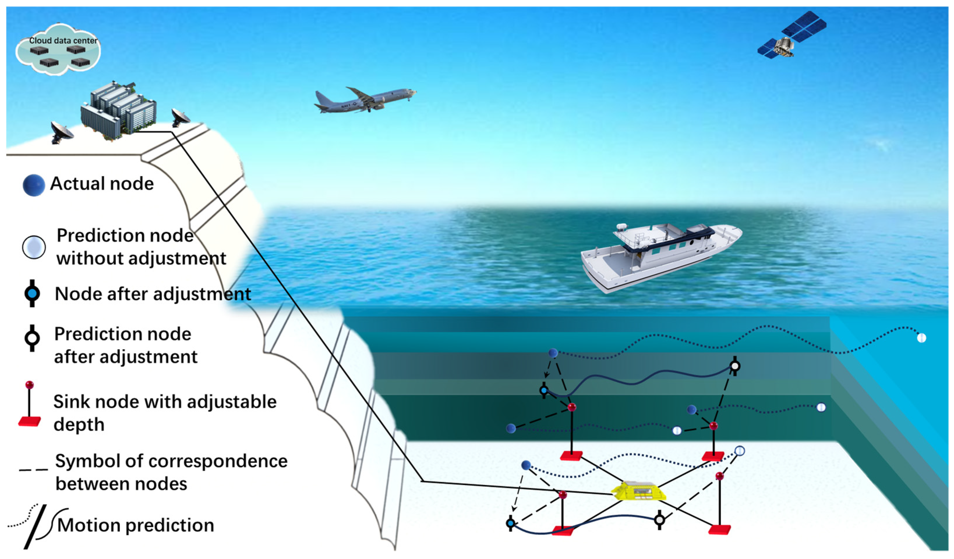
A plethora of research has been dedicated to static deployment and deployment strategies during the initial phase of network formation in UWSNs [28]. We focus on the performance variations in a UWSN throughout its operational lifecycle. Within UWSNs, the drift velocities of ocean currents vary with depth, leading to disparate drift distances for nodes at different depths. This variation consequently impacts the network topology and overall performance. Therefore, a node depth adjustment scheme based on node trajectory prediction and a swarm intelligence optimization algorithm are introduced, which encompass a stratified ocean current model, a node trajectory prediction model, and a node depth adjustment model, all aimed at enhancing network coverage and connectivity. The UWSN architecture primarily consists of ordinary nodes and sink nodes. Ordinary nodes constituted by Argo floats are utilized to collect environmental data [2]. In contrast, relay sink nodes are pivotal for information transmission within the UWSN [29], as depicted in Figure 1.
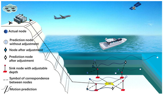
Figure 1.
Schematic diagram of node depth adjustment scheme based on ocean current prediction.
The layered ocean current model includes constructing the layered structure of ocean current and predicting ocean current parameters at different depths. Firstly, the ocean current properties at different depths are analyzed to determine the stratification standard. After that, the stratified ocean current data are used in the prediction model to form a stratified ocean current prediction model. The impact of ocean currents at different depths on node drift varies. Therefore, the trajectories of nodes at different layers can be derived by integrating ocean current stratification prediction data with kinematic equations. Finally, the optimal depth adjustment of nodes in the cycle is obtained by the SOA.
At the initial stage of the system, the original ocean current data are analyzed to determine the criteria for stratification. Then, based on these criteria, a deep stratification operation is carried out, and the layered ocean current model is established. The model covers the characteristics of ocean currents at different depth levels, including the rapid change of the surface layer and the relative stability of the deep layer.
Subsequently, the system adopts the ocean current prediction model constructed by the CNN–transformer hybrid neural network, which takes the data of the layered ocean current model as input to generate detailed and accurate ocean current prediction. The prediction model fully uses CNN’s advantages in extracting spatial features and combines the transformer’s global perception of long-time series data, which can effectively predict ocean currents’ spatial distribution and temporal changes.
Then, the system uses the node trajectory prediction model and ocean current prediction results to calculate the node trajectory in the future through the dynamic analysis of underwater nodes and the numerical incremental iteration method. This trajectory information is very important to guide the depth adjustment of nodes.
Finally, the system uses the SOA to intelligently adjust the node depth. This algorithm aims to improve network coverage and connectivity, simulates the seagull’s predation behavior strategy, and finds the best node depth adjustment scheme for ordinary nodes and sink nodes.
To sum up, the NAS-MP provides a complete solution, aiming to optimize the performance of the UWSN under dynamic ocean current change. This system integrates an accurate ocean current layered model, advanced ocean current prediction technology, node trajectory analysis, and intelligent optimization strategy to ensure the stable and efficient operation of a UWSN in complex marine environments.
The following key assumptions were put forward to ensure the feasibility and practicability of the model construction:
- (1)
- All nodes in the network were isomorphic and had the same communication radius and perception radius.
- (2)
- In the initial stage of the network, all nodes were randomly distributed in a square detection area with a side length of L.
- (3)
- Since the current velocity in the vertical direction was small, the influence of the current velocity in the vertical direction on the network was ignored.
4. Design of NAS-MP
4.1. Stratified Ocean Current Prediction Model
4.1.1. Introduction of Ocean Current Hierarchy Model
- A.
- Ocean Current Movement
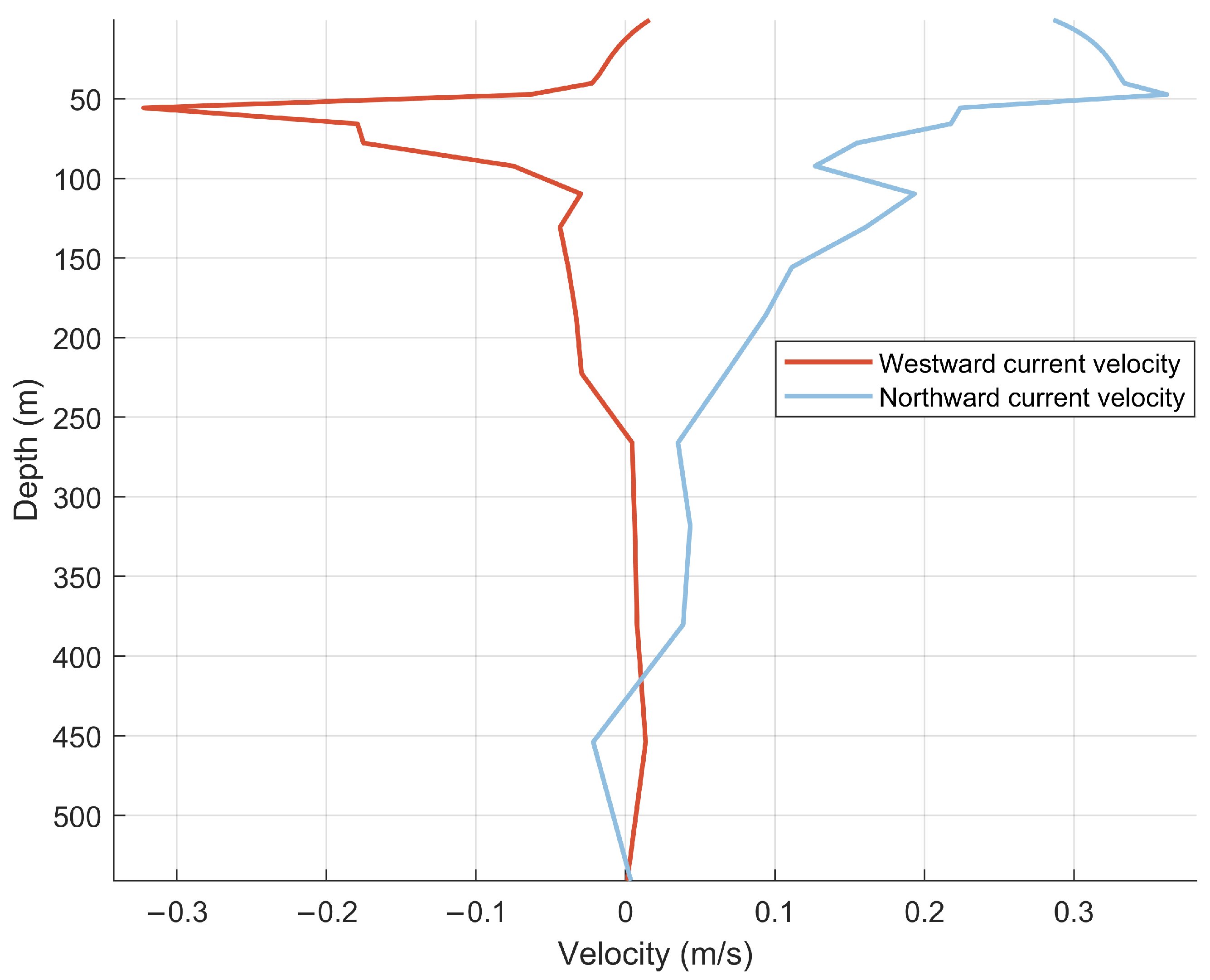
The multi-layer flow characteristics of the marine environment show its complex and dynamic characteristics. Ocean current varies with depth, as shown in Figure 2. Specifically, wind and temperature significantly affect the surface ocean currents, resulting in rapid changes in velocity and direction. In contrast, the deep ocean current changes more slowly and steadily. Based on this understanding, a layered ocean current model is proposed to accurately simulate the ocean current’s hierarchical structure and optimize underwater nodes’ depth layout.

Figure 2.
Variation trend of ocean current with depth.
In this model, the ocean area is unevenly divided into multiple layers according to depth, and each layer represents a specific depth range. In addition, to ensure the model’s accuracy, the shallow water area has a higher resolution to more accurately reflect the hierarchical characteristics of ocean currents. With the increase in depth, the layered resolution gradually decreases.
Depth-averaged currents can summarize the general characteristics of ocean currents but cannot accurately describe the situation of a single depth layer. Therefore, to more accurately predict the influence of each depth layer on the sensor nodes and optimize the node layout, this study constructed a layered ocean current model to provide more detailed ocean current information of different depth layers.
- B.
- Ocean Current Stratification Model
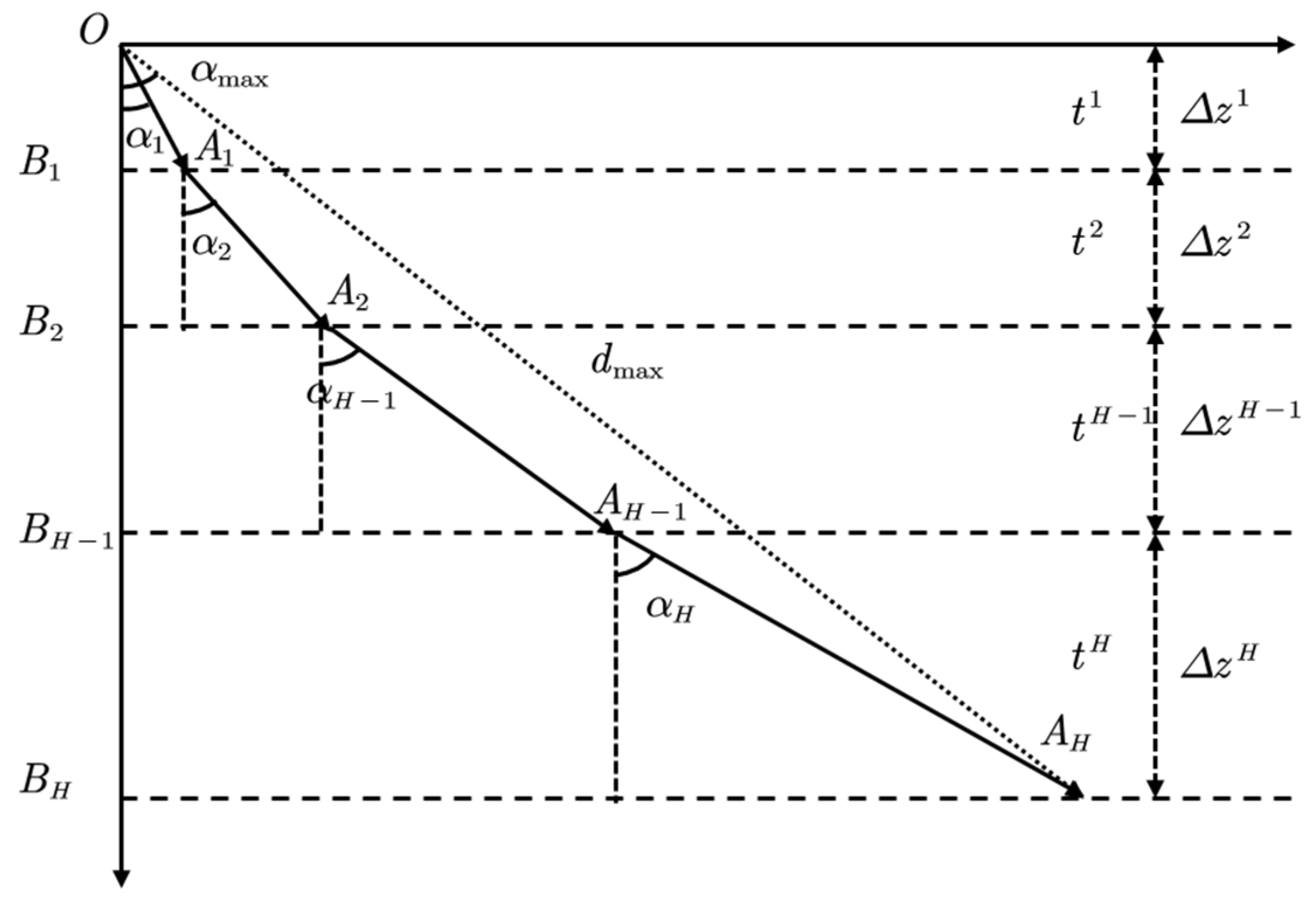
A key parameter was set to effectively implement stratified operation and build an accurate stratified ocean current prediction model: the error threshold of current velocity and direction in the layer, which was recorded as α [28]. This parameter could guide how to carry out effective depth stratification according to the actual observation data of the sea area to ensure that the ocean current change in the same layer was within the acceptable error range.
As shown in Figure 3, the sensor node was placed on the ocean current surface of the target sea area to make it sink freely. The tangent value of the maximum angular deviation αmax and the maximum horizontal displacement dmax were as follows:
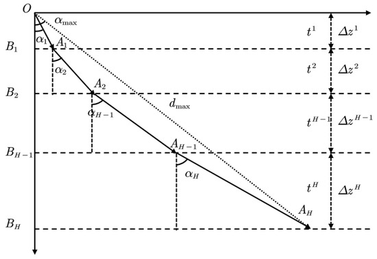
Figure 3.
Depth displacement surface.
Assuming that the vertical sinking speed of nodes was , the interlayer sinking time of nodes was . Therefore, and could be obtained, and Equations (1) and (2) could be transformed and simplified to obtain the following:
where is the depth of the ocean current, H is the number of ocean current layers, is the vertical sinking speed, and and are the maximum velocity error and maximum flow angle error in each layer, respectively.
Therefore, the stratification operation of ocean current was set by the maximum angular deviation αmax and the maximum horizontal displacement dmax experienced by the node’s free sinking or rising so that each layer’s maximum velocity error and maximum flow angle error satisfied their relationship. The maximum horizontal displacement dmax of nodes could be obtained from the sensor network’s deployment area and the node depth adjustment period. The layered ocean current model could give full play to the data information in shallow waters and effectively delete redundant information in deep waters.
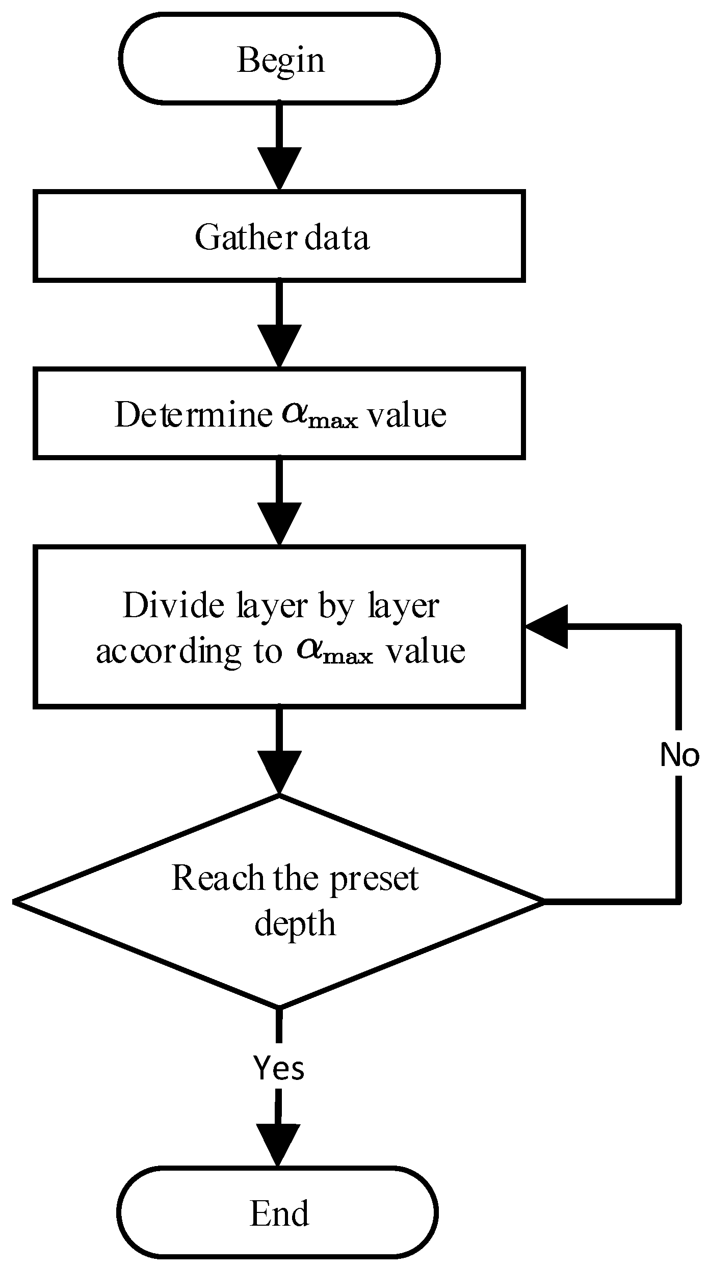
Ocean current stratification operation included the following steps:
- (1)
- Data collection: Collect historical and real-time ocean current data of the target sea area, including information such as velocity and direction.
- (2)
- Data analysis: Analyze the ocean current data to determine the maximum error αmax to meet the sensor network’s performance requirements.
- (3)
- Divide down layer by layer: From the surface layer, divide the depth level by layer according to the αmax value.
- (4)
- Complete layering: Repeat step 3 until the predetermined maximum depth is reached, and complete the layering operation.
Thus, a hierarchical model could be established through the above process, which could reflect the actual ocean current changes and meet the performance requirements of sensor networks, as shown in Figure 4. This model could guide the more accurate depth adjustment of the UWSN nodes to optimize the network performance.

Figure 4.
Flow chart of the stratified operation of ocean current.
4.1.2. Ocean Current Prediction Model
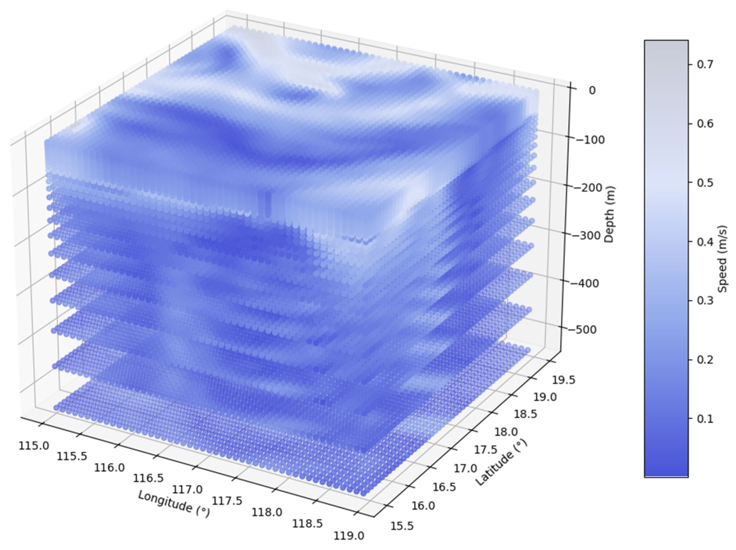
The ocean current prediction model was the basis of the periodic adjustment of nodes. However, there were differences in ocean current velocity at different depths, and the stratified ocean current is shown in Figure 5. Only by accurately grasping the future changes in regional ocean currents could the trajectory of nodes be accurately predicted. Only by adjusting the nodes’ position could the sensor network be effectively optimized.
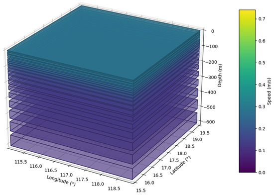
Figure 5.
Schematic diagram of the stratified ocean current model.
Therefore, this study used the CNN–transformer hybrid neural network to predict ocean currents, elucidating ocean current change’s spatial and time series characteristics. Before introducing the CNN–transformer model, the CNN and transformer models are briefly discussed.
- A.
- Convolutional Neural Network (CNN)
A CNN is a neural network structure proposed by LeCun et al. [30] that includes an input layer, an output layer, and a hidden layer. The input layer transmits the original data to the first hidden layer and the output layer generates the output of the given input. The hidden layer includes convolution, pooling, and full connection layers, among which, convolution and pooling layers are the core, which can effectively extract features, reduce the number of parameters, and speed up training.
The convolution layer extracts features from the input data and scans the input data using a set of convolution kernels through a sliding window. Equation (5) describes this process:
where represents the input data, represents the feature map after convolution, w represents the weight of the convolution kernel, p represents the current position of the sliding window, n represents the position of elements in the convolution kernel, and R represents the area covered by the convolution kernel.
The convolution layer can capture local features efficiently and maintain the sensitivity of the spatial hierarchical structure through weight sharing and local connections.
After the convolution layer, it is usually the pooling layer that aims to reduce the spatial dimension of the feature map, reduce the amount of calculation, control over-fitting, and keep the main feature information. The common pooling operations include average pooling and maximum pooling.
The activation function introduces non-linearity, which promotes network learning and expresses more complex functions. After many convolutions and pooling layers, the fully connected layer maps features to the space of sample labels. Through this layered architecture, a CNN gradually extracts the hierarchical features of input data to realize classification or other task prediction.
- B.
- Transformer
The transformer is a neural network architecture proposed by Vaswani et al. [31] in 2017. Unlike the traditional RNN or CNN, it completely relies on the attention mechanism to process sequence data and does not use recursive and convolution layers. This design gives the transformer higher computational parallelism when dealing with long sequence data and can achieve excellent results quickly.
The transformer model consists of an encoder and a decoder, each part containing several identical layers. Each layer has a multi-head attention mechanism and a fully connected feed-forward network. Its core idea is to use the self-attention mechanism to enhance the model’s attention to different parts of the input data. Hence, it can perform well in sequence-to-sequence tasks.
The scaled dot-product attention is the core of the transformer’s self-attention mechanism. Its core idea is that for a given query, key, and value, the attention function outputs the sum of weights by calculating the dot product of the query and all keys, and the mathematical expression is shown in Equation (6):
where Q, K, and V represent the matrix of query, key, and value, respectively; is the scaling factor; and T is the dimension of the key.
The multi-head attention disperses the attention of the model to different positions, pays attention to different parts of the input at the same time, and captures different features, as shown in Equations (7) and (8):
where WQ, WK, and WV represent projection matrices, which generate different subspaces of query, key, and value matrices, respectively. WO stands for projection matrix of the multi-head output , , , and , =.
In the transformer model, each layer of the encoder and decoder contains a fully connected feed-forward network, which is applied to each position independently. It consists of two linear transformations and a ReLU activation function, as shown in Equation (9).
Since the transformer does not adopt a circular structure, it cannot automatically process the position information of data like an RNN. Therefore, when inputting data, the positional encoding is adopted so that the model can use the sequence information, as shown in Equations (10) and (11):
where pos is the position and h represents the dimension.
- C.
- CNN–Transformer
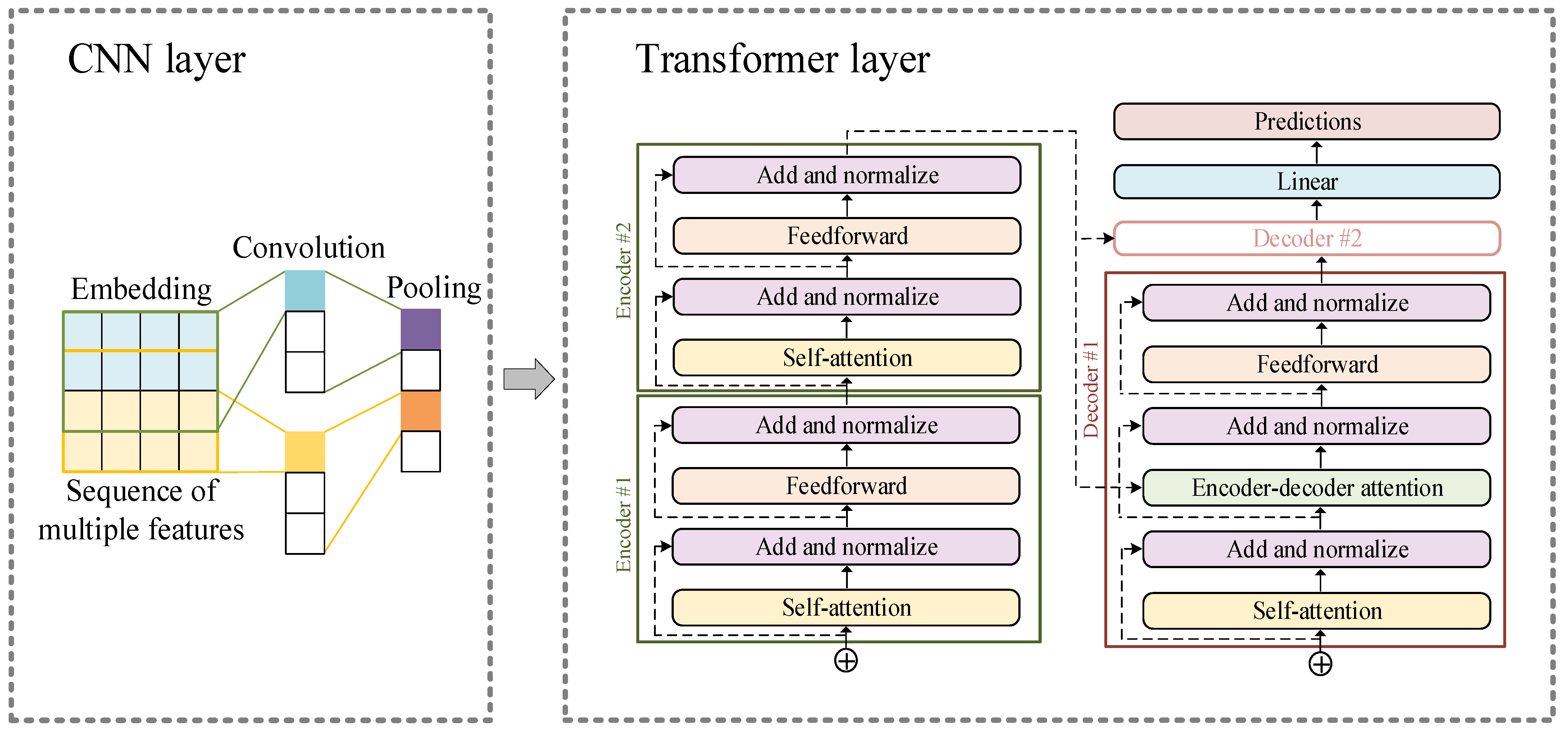
The CNN–transformer hybrid network model was used for regional ocean current prediction, as shown in Figure 6. Firstly, the ocean current data was processed by the CNN and the spatial features were extracted through multiple convolution and pool layers. The convolution layer captured local features through the convolution kernel of a sliding window. In contrast, the pooling layer reduced the feature dimension, improving computational efficiency and reducing over-fitting. After convolution and pooling, the data contained important information about ocean currents’ spatial distribution. Then, the data were position-coded before the encoder structure of the transformer model to provide time series position information. The encoder processed the feature sequence with position coding and captured the long-distance dependence in the data through self-attention. The decoder further processed the encoder output and generated a prediction sequence, considering the encoder and previously decoded output. At the end of the hybrid model, the decoder output the final ocean current prediction result through flattening, dropout, and a full connection layer.
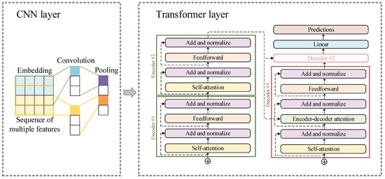
Figure 6.
The model architecture of the CNN–transformer model.
In the model, the CNN captured the spatial details of ocean current data, while the transformer dealt with the long-distance dependence of time series. Combining these two abilities of detail capture and global perception improved the model’s understanding of ocean currents’ dynamic changes. The combination of the CNN’s local perception and the transformer’s efficient parallel processing improved the efficiency and flexibility of the model in processing large-scale ocean current data. The ocean current prediction model is shown in Figure 7.
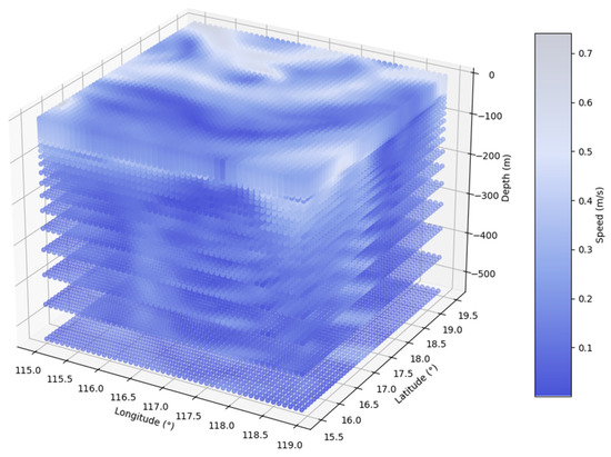
Figure 7.
Ocean current prediction model.
4.2. Motion Trajectory Prediction of Sensor Nodes
4.2.1. Dynamic Analysis of Underwater Node
The existence of underwater ocean currents leads to the constant drift of underwater nodes. For a node with a specific depth, there are three forces: self-weight, buoyancy, and water thrust [32].
First, the calculation of gravity is shown in Equation (12):
where represents the force of gravity, represents the density of the node, represents the volume of the node, and represents the acceleration of the earth’s gravity. Gravity is the main sinking force, which causes the node to accelerate downward. The buoyancy is used to counteract gravity, and its calculation is shown in Equation (13):
where is the density of seawater, is the node’s volume, and is the terrestrial gravitational acceleration.
In addition to gravity and buoyancy, the node is also acted on by another force, pushing the node to move in the direction along the ocean current’s speed, which is one of the reasons leading to node drift, and its calculation is shown in Equation (14):
where k is a constant, is a shape factor, AC is the cross-sectional area of the node facing the water flow, is the water flow velocity, and is the projection of the node velocity on the same plane as the water flow velocity.
For the node located at the coordinate (x, y, z), the velocity in the horizontal direction can be expressed by Equation (15) and the acceleration can be expressed by Equation (16):
From Newton’s second law, the equilibrium equation can be obtained as shown in Equation (17):
Then, the dynamic system equations of nodes in the x-y plane can be obtained, as shown in Equations (18) and (19):
where and and represent the water flow components in the x and y directions, respectively.
4.2.2. Numerical Solution
Supposing that the current velocities and and seawater density are constant. In that case, the above kinematic equations can be simplified to two linear independent second-order differential equations for an analytical solution, as shown in Equations (20) and (21):
where t0 is the reference time, x0 and y0 are the positions of nodes at t0, and and are the velocities of nodes at t0. In addition, on the horizontal plane, the ocean current velocities and and seawater density at time t0 at coordinates (x, y, z) are all obtained by the ocean current prediction model established before.
Subsequently, the numerical incremental iteration method solves the above differential equations to obtain the node’s position.
Assuming a fixed time step, the seawater density , ocean current velocities and , and current direction remain constant during the period . Therefore, Equations (20) and (21) can calculate a time step. If the positions xj, yj, and zj and the velocities and of the nodes at tj are known, then in the period [, ] ( = ), , , and all remain unchanged, while the positions xj + 1 and yj + 1 of the nodes at tj + 1 can be expressed by Equations (22) and (23):
In addition, by simply differentiating Equations (22) and (23) in time and replacing t0 with , the speed of the node at tj+1 can be obtained from Equations (24) and (25):
The above method can predict the node’s future motion trajectory using the node’s initial state and the underwater environment parameters combined with the layered ocean current prediction model [28].
4.3. Node Depth Adjustment Scheme
Affected by ocean currents, nodes with different depths drift to different degrees with time, which leads to two problems. First, the network coverage decreases, making it more difficult to detect the target area. Second, node drift at different depths changes the topology of the UWSN, which may lead to node link interruption. It is necessary to optimize the performance of the UWSN by regularly adjusting the node depth. Therefore, a node depth adjustment scheme is proposed.
4.3.1. Coverage and Connectivity Mathematical Models
Assuming that the target detection area is three-dimensional, the number of nodes is N and the communication radius is r. The node set is symbolized as follows:
where represents a monitoring area with the node (xo, yo, zo) as the center and the radius r. Assuming that the monitoring area is evenly divided into a × b × c spatial nodes and the coordinates of the spatial points are (xi, yi, zi), the distance between the target point and the nodes can be expressed by Equation (27):
In addition, assuming that the event that a node covers a position point in the target area is defined as ci, the probability of this event is , that is, the probability that a node nodeo covers this position point (xi, yi, zi) can be expressed by Equation (28):
The CoverageRatio of the area coverage of all nodes in the target monitoring environment is defined as the ratio of the coverage range of the node set to the monitoring range, as shown in Equation (29):
In addition, the ConnectRatio of the network is defined as the ratio of the nodes’ number Nc that can communicate with the sink node through single-hop or multi-hop to the total number of nodes N, as shown in Equation (30):
The ultimate goal is to find a group of nodes to maximize the network’s coverage and connectivity. Next, the SOA is used to find the optimal solution to achieve this goal.
4.3.2. Seagull Optimization Algorithm (SOA)
The SOA is a new swarm intelligence optimization algorithm proposed by Gaurav Dhiman and Vijay Kumar in 2018 with strong global search ability and low computational complexity. The algorithm simulates seagulls’ migration and attack behavior [8]. The former affects global exploration and the latter affects local development. Through this algorithm, the period adjustment depth of each node can be determined to optimize the network’s coverage and connectivity during the period.
- A.
- Migratory Behavior
At this stage, the following three points should be considered: avoiding collision, moving to the best neighbor, and keeping close contact with the best search agent.
In order to avoid collision with neighboring seagulls, an additional variable is introduced to calculate the position of the search agent, which is expressed by Equation (31):
where is the position without collision with other search agents, is the current position of the search agent, s is the current iteration number, and A is the moving behavior of the search agent in a given search space, as shown in Equation (32):
where x = 0, 1, 2, …, Maxiteration. In addition, fc is introduced to adjust the changing frequency of A so that it gradually decreases linearly from fc to 0.
Under the condition of ensuring no collision with neighbors, the search agent moves in the direction of the best neighbor, as shown in Equation (33):
where represents the position vector of the search agent relative to the optimal search agent . B’s behavior is random to strike a proper balance between exploration and development. The calculation of B is shown in Equation (34):
where rd is a random number with a value range of [0, 1].
Finally, the search agent can update its position according to the optimal search agent, as shown in Equation (35):
where represents the distance between the search agent and the optimal search agent.
- B.
- Aggressive Behavior
Seagulls can maintain their height by adjusting the attack angle and speed during migration, and their posture can be adjusted by changing their wings and weight. When seagulls prey on prey, they will spiral into the prey in the air and attack.
The following equation can be used to describe the specific position of the node represented by seagulls in three-dimensional space:
where r represents the radius of each turn of the spiral, is a random number with a value range of [0, 2π], u and v are constants used to define the shape of the spiral, and e is the base of the natural logarithm. The algorithm controls the spiral radius r by adjusting u and v. The updated position of the search agent can be calculated by Equation (40):
Among them, carries the optimal solution and is responsible for adjusting the positions of other search agents.
4.3.3. Improved Seagull Optimization Algorithm
- A.
- Tent Chaotic Mapping Initialization Strategy
The initial positions of seagulls in the basic Seagull Optimization Algorithm (SOA) are random, which may lead to an uneven distribution of seagull positions, thereby reducing population diversity and optimization speed. Due to the greater advantages of tent chaotic mapping [33] in terms of ergodicity, uniformity, regularity, and iteration speed, this study adopted a chaotic mapping strategy to improve the initialization process of the seagull population. The function expression for generating chaotic particle sequences using tent mapping is shown in Equation (41).
- B.
- Fast Elitist Non-Dominated Sorting
Fast elitist non-dominated sorting [34] is an algorithm used for multi-objective optimization problems that improves optimization performance by identifying and retaining the best-performing individuals in the population. The algorithm first performs non-dominated sorting on the population, dividing individuals into multiple fronts based on their non-dominated levels. Within each front, the crowding distance of individuals is calculated using an elitist strategy. This approach prioritizes the retention of individuals with higher non-dominated levels and larger crowding distances, thereby maintaining population diversity while ensuring the accuracy and effectiveness of the optimization direction.
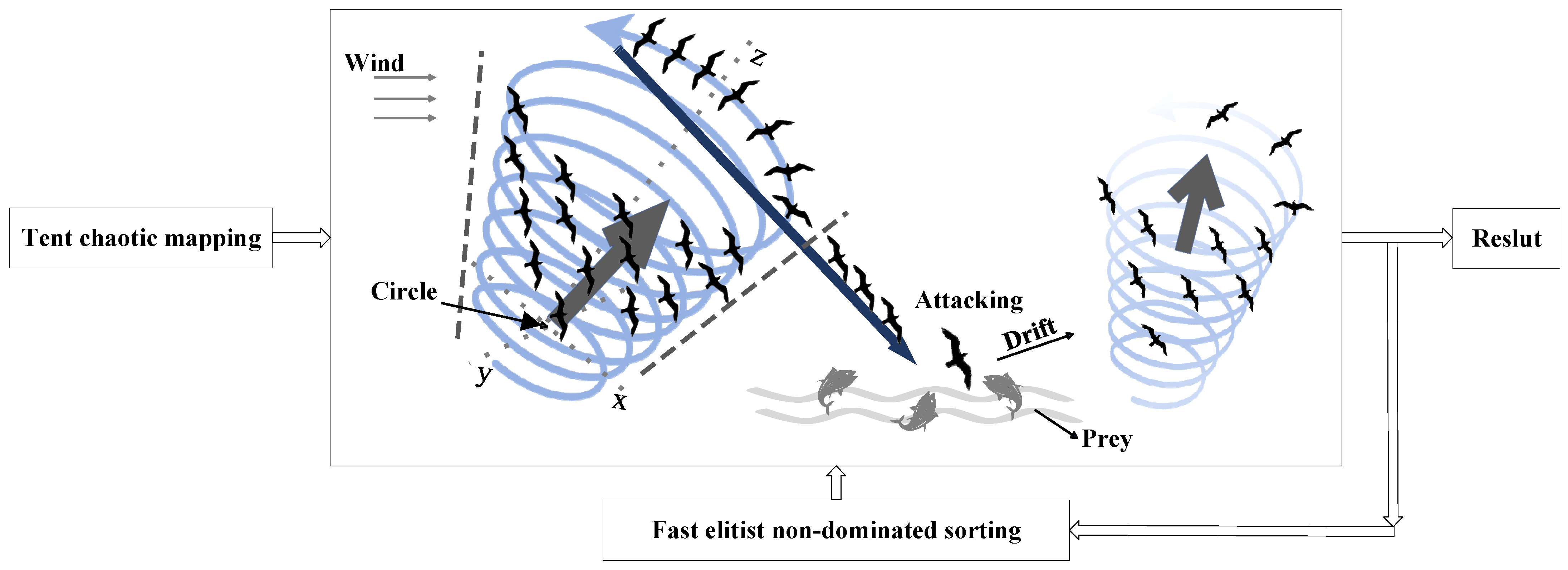
The improved Seagull Optimization Algorithm incorporated a tent chaotic initialization strategy and fast elitist non-dominated sorting, enabling the algorithm to initialize a diverse population and quickly find dominant solutions when solving multi-objective optimization problems. The schematic diagram of the improved SOA is shown in Figure 8. According to the above description, Algorithm 1 proposes an algorithm for adjusting the depth of underwater sensor nodes based on the improved SOA.
| Algorithm 1 Depth adjustment algorithm of underwater nodes based on the improved SOA |
| Input: Node position coordinates, node predicted trajectory coordinates, total number of nodes N. Output: Optimal adjustment depth of nodes. 1: Initialization parameter setting 2: Using tent chaotic mapping to determine the positions of N nodes in a sensor network within a specified space 3: While (range < MAXiteration) do 4: Calculating the fitness value of each search agent 5: Generate random number rd, which is used to determine migration and attack behavior 6: Generate random number k for spiral behavior 7: Calculate the position update r of spiral behavior 8: Calculate the distance between each search agent and the optimal search agent 9: Using spiral and random behavior to update the search agent’s position in the x, y, z plane 10: Using a non-dominated quick elite sort based on the updated position and the current optimal position to update the position of each search agent 11: Update iteration counter 12: End while |
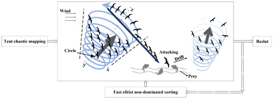
Figure 8.
The schematic diagram of the improved SOA.
5. Simulation Results
5.1. Ocean Current Data Source
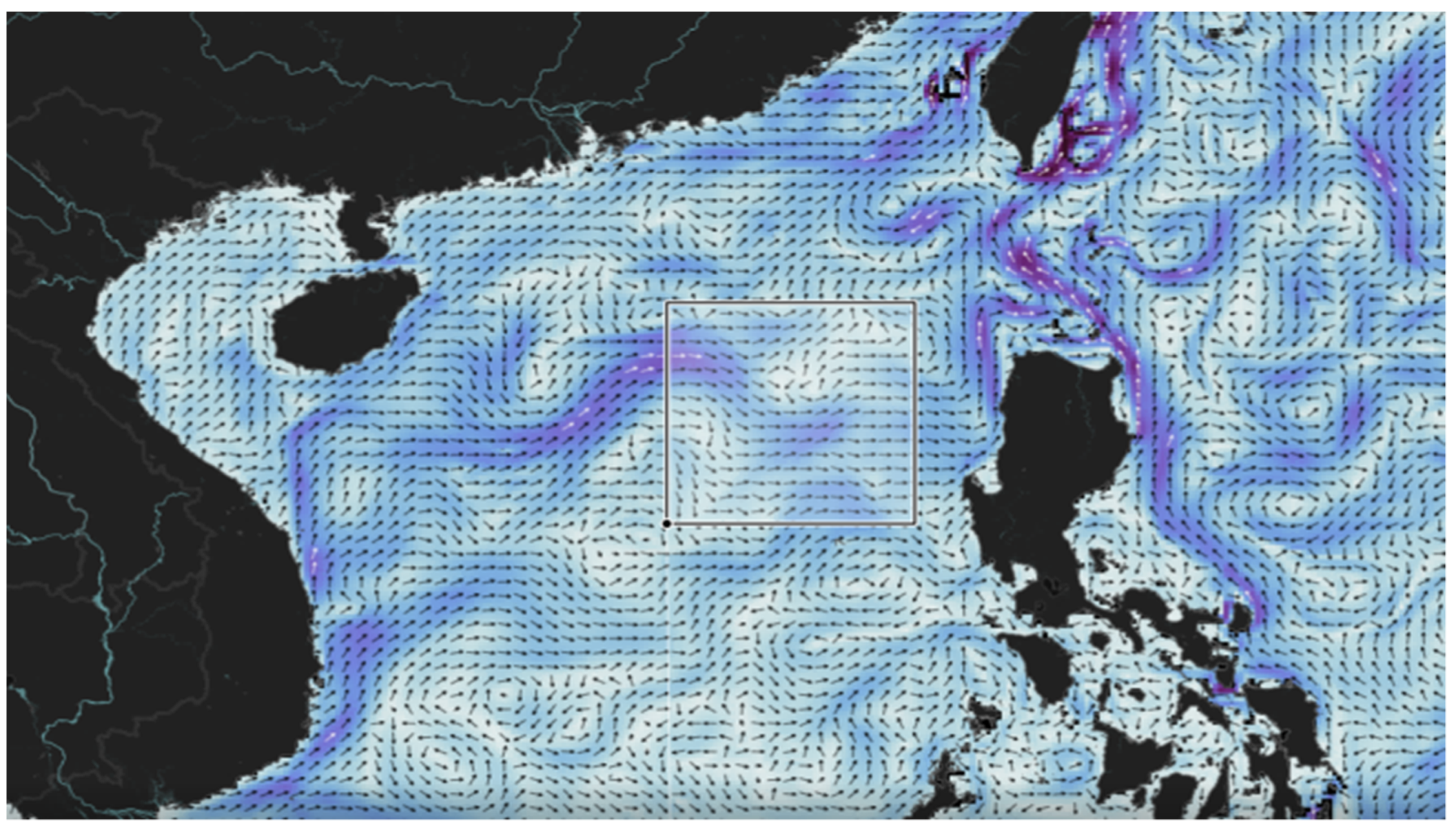
The ocean current data used in this study were obtained from the Copernicus Ocean Data Center [35], and data from 1 January 2021 to 1 January 2024 were obtained. In order to meet the needs of the UWSN, ocean current data sets between 115° E and 119° E and 15.5° N and 19.5° N were downloaded. As shown in Figure 9, these data were used as historical data to establish an ocean current prediction model and provide support for simulating the sea area of UWSN nodes.

Figure 9.
Distribution map of ocean current in the South China Sea (the box in the figure is our selected experimental area).
Historical ocean current data were preprocessed and spatially interpolated and an ocean current data model covering part of the South China Sea was established. This part of the data was used to train the ocean current forecasting model and verify the feasibility of the node adjustment scheme.
5.2. CNN–Transformer Neural Network Structure and Model Training
The network structure of the ocean current prediction model included six layers: input layer, convolutional neural network layer, transformer layer, dense connection layer, discard layer, and output layer. Table 1 summarizes the model’s frame structure, including the name of each level and its output shape.

Table 1.
The numerical changes of each layer in the CNN–transformer model.
The input layer data came from the ocean current data model, divided into an 80% training and a 20% verification set. The data were input in tensor form with the size of (None, 80, 256), where None represents the batch size, 80 represents the input window size of the time series, and 256 represents the number of features in the data. The data were first processed by the CNN layer, which used two convolution kernels with different sizes and the ReLU activation function to extract features from the input data automatically. Subsequently, the feature dimension was raised to the hidden layer’s size through the dense connection layer to increase the model’s feature extraction ability. Before entering the transformer layer, in order to avoid over-fitting, 20% of data points were discarded. The transformer layer consisted of two encoder layers and two decoder layers, and the multi-head self-attention mechanism was set to 4, aiming to extract more feature information from the time series of ocean current data. After the transformer layer processing, the characteristic length of the data became the size of the prediction window, that is, 40, which represented the size of the prediction window of the time series. Finally, the feature dimension of the data was mapped back to the original feature dimension size through the output layer. Hence, it could obtain the final prediction result.
In the training process, the Adam optimizer was adopted, and the loss function was defined as the mean square error (MSE) between the predicted label (ocean current velocity with dimension information of time and space) and the real label. This index could effectively evaluate the degree to which the model fit the real data. The Adam optimizer adopted an adaptive learning rate adjustment strategy, which had a large initial learning rate and helped accelerate the convergence process. With the training, the learning rate gradually decreased, which helped the model approach the local optimal solution stably.
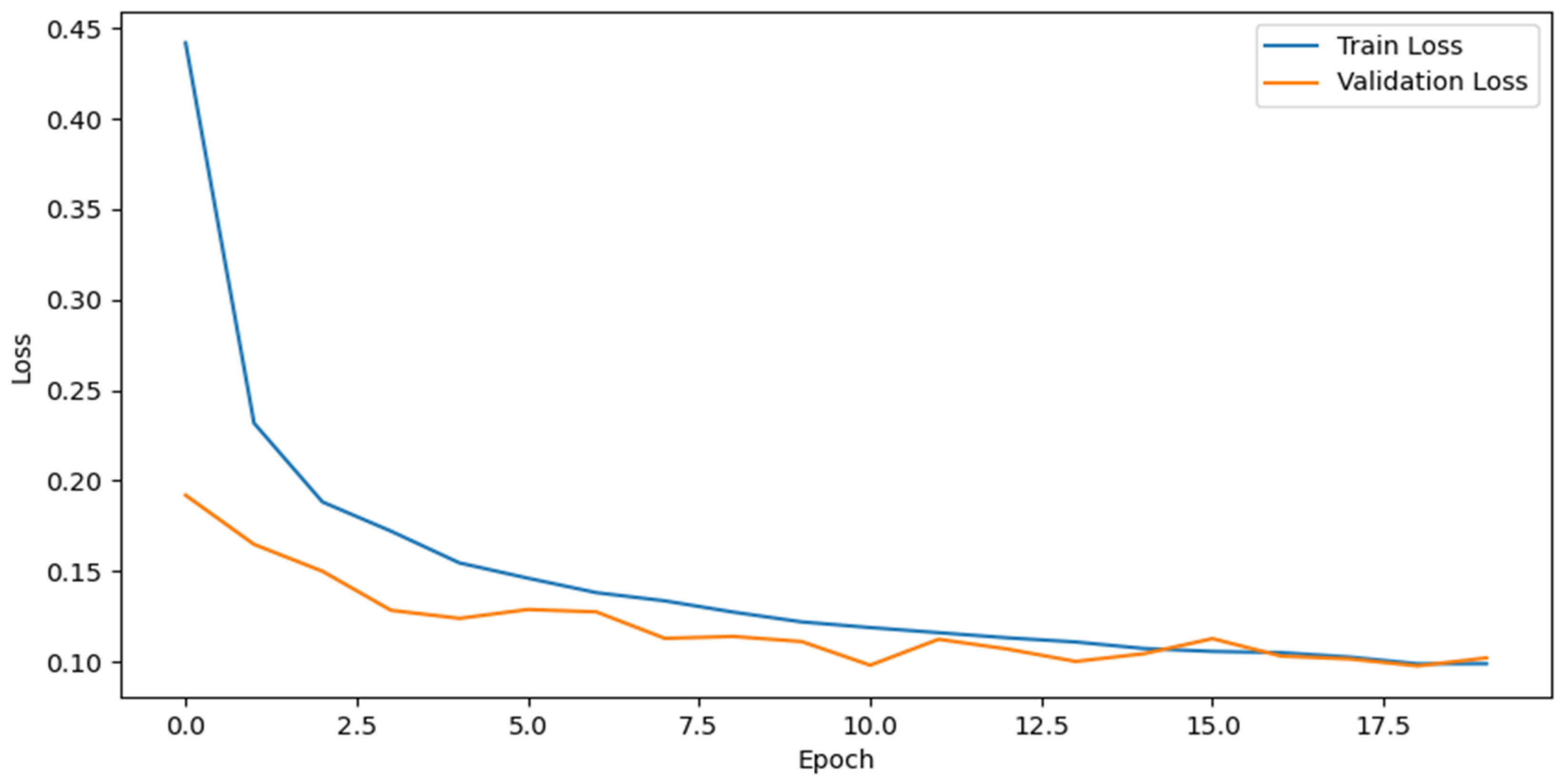
Figure 10 shows the change in loss after 20 trainings. As the number of training iterations increased, both the training loss and the verification loss gradually decreased, indicating that the model’s performance continued to improve. At the 18th epoch, the model reached the minimum loss. However, too many training cycles could lead to over-fitting the model, increasing the loss.
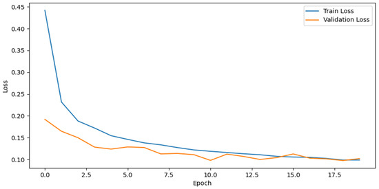
Figure 10.
Changes in loss after 20 training cycles.
5.3. Using SOA to Optimize and Adjust the UWSN
A sea area of 600 m × 600 m × 600 m was randomly selected from ocean current data as the activity and detection area of the UWSN. The initial positions of all ordinary nodes were evenly distributed in this area, while the bases of the four sink nodes were evenly placed at the bottom of the water. The depth layer where the sink nodes were located could be adjusted adaptively according to the needs of the network structure. Please refer to Table 2 for the specific parameter settings of the model.
Table 2.
System symbols.
A 10-day simulation operation of the UWSN was conducted in the sea area. At the beginning of each cycle, the depth of the node was adjusted. Specifically, the predicted trajectory of nodes was analyzed to determine the best node adjustment strategy in each cycle, and then the network coverage and connectivity changes were calculated. In addition, the average value of these two metrics within the time frame was adopted as the optimization objective. A tent chaotic map was utilized to generate the initial solution space and compute the initial fitness. In the iterative process, the SOA algorithm generated a series of new non-dominated solutions. Then, the non-dominated quick sorting method based on the elite strategy was used to sort the old and new solutions. After completing the iteration, a boundary composed of dominant solutions could be obtained. According to the preset optimization weights, the optimal solution could be selected at the beginning of the cycle to determine the optimal adjustment strategy.
In this study, the network nodes were constructed using real data run in the sea area. According to the proposed optimal adjustment strategy, the adjustment scheme of nodes at the beginning of each cycle depended on the influence of predicted future ocean current changes on node movement. Therefore, the accuracy of the adjustment scheme and the actual effect of network optimization were affected by the accuracy of ocean current prediction. Real ocean current data were used instead of forecast data to verify the feasibility of the periodic node depth adjustment scheme to improve network performance.
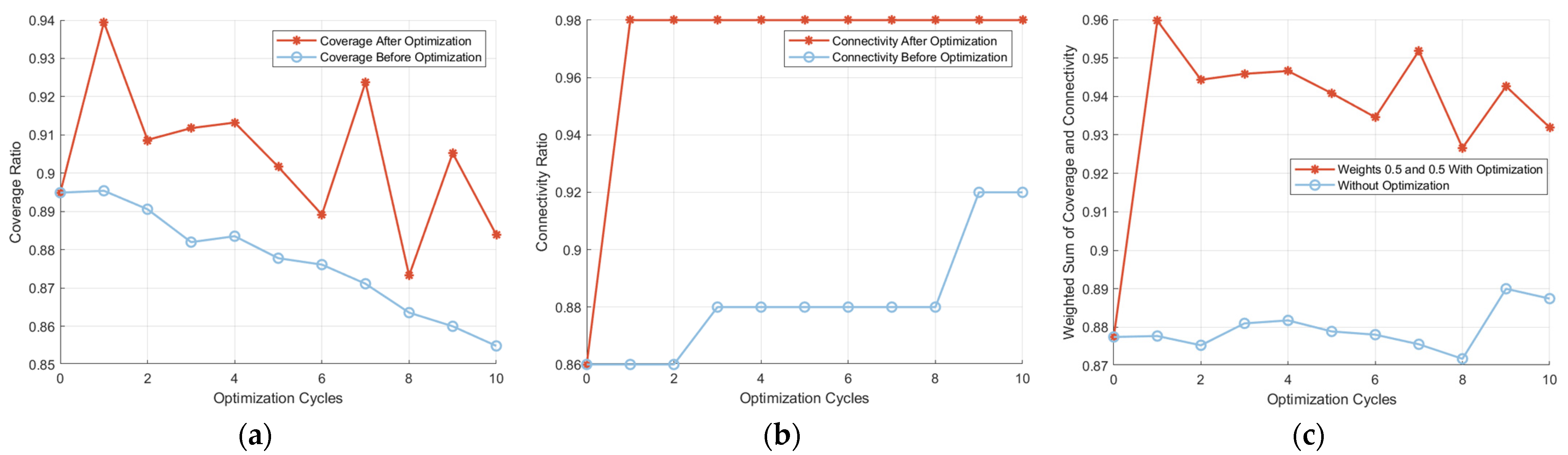
Figure 11 shows the performance changes of the UWSN when the optimal weight ratio of coverage and connectivity was set to 5:5. With the operation of the network, the influence of ocean currents on sensor nodes led to the continuous drift of nodes, gradually reducing the network coverage. Implementing the optimized depth scheme reduced the extent of this decline, as shown in Figure 11a. After introducing the optimization adjustment strategy of periodic depth adjustment, the node distribution was obviously improved, and the network’s average coverage was significantly improved compared with the unoptimized state. However, the performance fluctuation in individual periods was because the current periodic depth adjustment scheme only considered the network performance change before the next node adjustment and did not consider the influence of subsequent periods. Due to the spatial difference of the real-time ocean current environment, the network performance changes were inconsistent before and after optimization.
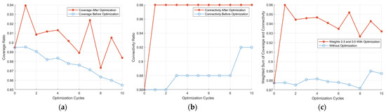
Figure 11.
Network performance changes with running time under actual ocean current: (a) coverage; (b) connectivity; (c) comprehensive performance.
In addition, the overall movement trend of sensor nodes with only the depth adjustment function used for sea area detection tasks was consistent with the current ocean environment, which was also the main reason for the network performance fluctuation. As far as network connectivity is concerned, as shown in Figure 11b, the network connectivity obviously improved after the introduction of the optimization adjustment strategy. In addition, the optimized network connectivity rate could always be maintained at a high level because the sink nodes could adjust their depth layer according to the distribution of nodes. Furthermore, the coverage and connectivity before and after network optimization were multiplied by 0.5 and then they were added together to comprehensively evaluate the change in network performance. As shown in Figure 11c, the comprehensive performance of the optimized network was significantly improved, and the performance improvement effect was more significant with the increase in network running time.
During the periodic operation of the sensor network, ocean currents continuously affected the network’s coverage and connectivity. Since the node communication employed a multi-hop transmission method, it possessed good interference resistance against ocean currents. Therefore, by decreasing the connectivity optimization weight from 0.5 to 0.1 and increasing the coverage optimization weight from 0.5 to 0.9, we periodically operated the network to collect optimization data.
Figure 12 shows the influence of the optimization weight ratio of coverage and connectivity on the comprehensive performance. Under different weight ratios, the initial deployment of nodes was consistent. Because of the different settings of the weight ratio, the optimal solution selected after each iteration was different, which led to a difference in network performance. Although the network performance changes were different under different settings, the overall trend significantly improved compared with the unoptimized network. The proposed optimization scheme was highly versatile and could improve performance under different network requirements.
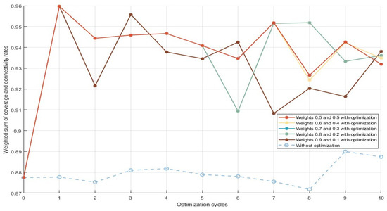
Figure 12.
Influence of optimized weight on network comprehensive performance under actual ocean current.
5.4. Comprehensive Performance Analysis of the Model
To verify the feasibility of the periodic node depth adjustment scheme for network performance optimization, real ocean current data were used instead of predicted ocean current data to eliminate the influence of deviation between predicted data and real data on network performance. Firstly, the predicted ocean current data were used to predict the periodic movement trajectories of the nodes. Then, based on these trajectories, the optimization algorithm generated a periodic depth adjustment scheme. Finally, the nodes were placed in the sea area and constructed with real ocean current data. The depth adjustment scheme generated from the predicted data was executed. This process allowed us to observe changes in network performance and simulate a more realistic application scenario.
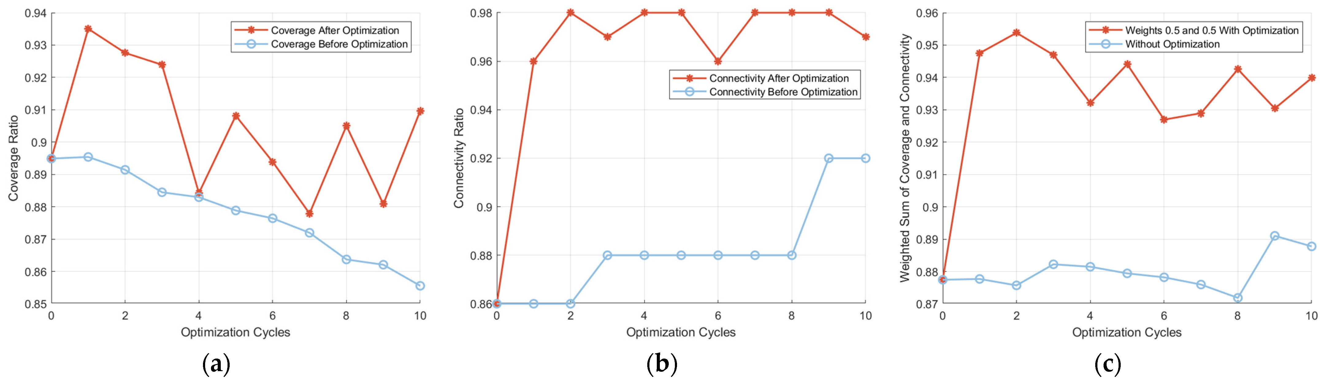
Figure 13 shows the influence of the adjustment scheme generated by using the predicted data on the network performance when the optimization weight ratio of coverage and connectivity was set to 5:5. The results show that after optimization and adjustment, the network’s performance was significantly improved compared with that without adjustment. However, compared with Figure 11, the optimized network’s performance was slightly reduced due to some errors between the predicted ocean current data and the actual ocean current.
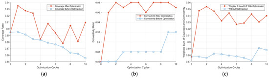
Figure 13.
Network performance changes with running time under predicting ocean currents: (a) coverage; (b) connectivity; (c) comprehensive performance.
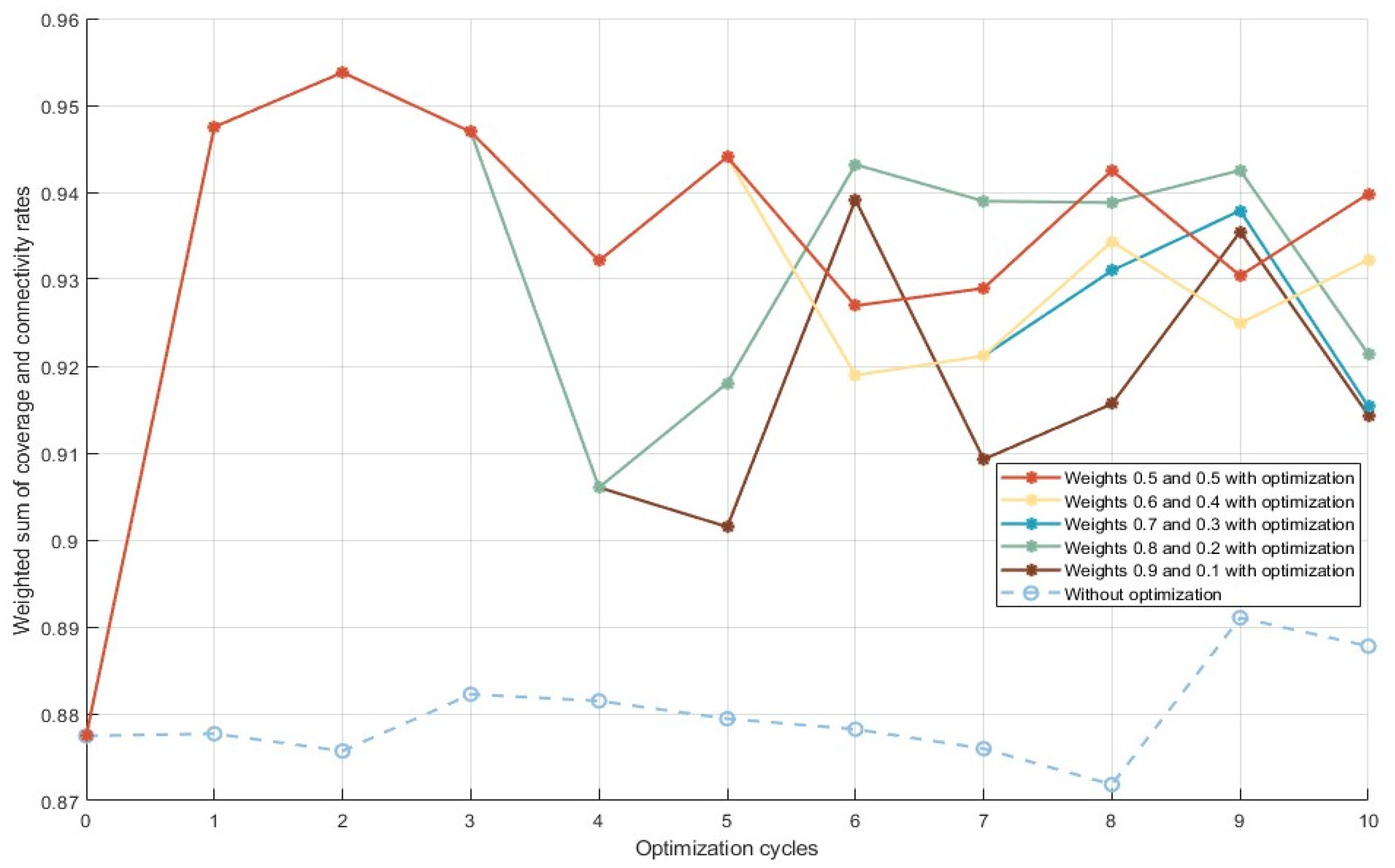
In addition, Figure 14 shows the influence of adjusting the optimized weight ratio on the comprehensive performance. Compared with Figure 12, although the network performance after optimization was slightly reduced, compared with the situation without optimization and adjustment, the network performance after adding nodes was significantly improved. To sum up, our periodic node depth adjustment scheme could effectively weaken the influence of ocean currents on the UWSN, thus significantly improving the network performance in long-term operation.
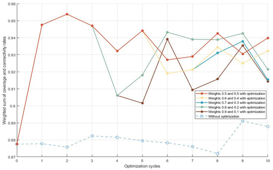
Figure 14.
Influence of optimized weight on network comprehensive performance under predicting ocean currents.
5.5. Comparative Analysis of Node Distribution
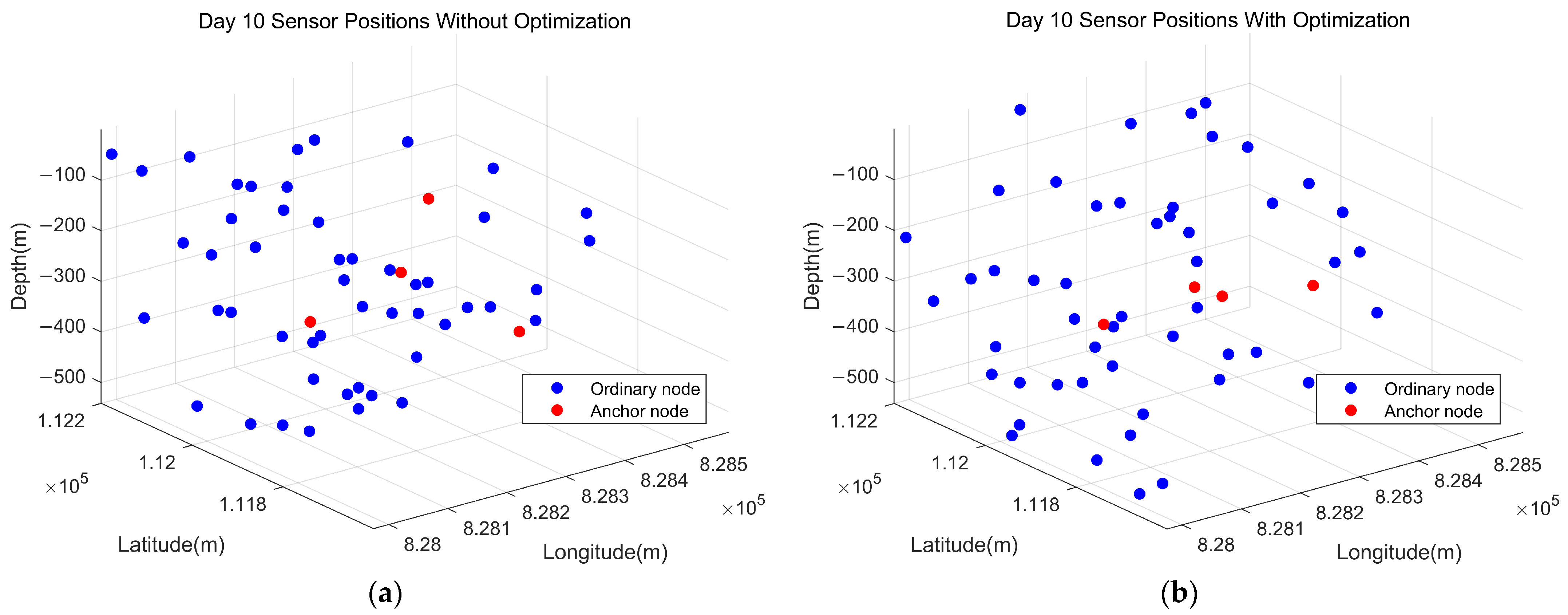
We investigated the adjustment strategies for common nodes affected by ocean currents, focusing on dynamic node adjustment during the network’s operational process in response to ocean current movement. Figure 15 presents a comparative analysis of the node distribution status within a UWSN subjected to dynamic ocean currents, contrasting the scenarios with and without applying the proposed adjustment scheme. Figure 15a illustrates that the UWSN without depth adjustment exhibited the characteristics of a smaller coverage area and uneven distribution, manifesting as a smaller coverage area with regions of excessive node aggregation juxtaposed against areas of sparse deployment, which resulted in the formation of detection voids in the deployment space because the upper ocean currents were faster, while the deeper currents were more moderate in speed. On the other hand, the adjusted UWSN demonstrated a larger coverage area and a more uniform distribution of nodes compared to its unadjusted counterpart, as depicted in Figure 15b. Attributed to our node depth adjustment scheme, based on ocean current prediction, it could enhance the network’s coverage by adjusting node depths while ensuring connectivity.
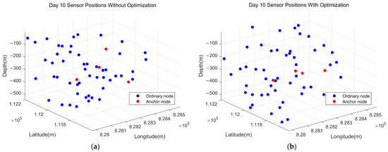
Figure 15.
Comparative analysis of UWSN distribution: (a) without depth adjustment of nodes during the networking process; (b) with depth adjustment of nodes during the networking process.
6. Conclusions
We studied the periodic depth adjustment model of mobile nodes based on the stratified prediction of ocean currents. Firstly, the layered prediction model of current realized the stratification of regional current based on error threshold, which ensured the prediction accuracy and reduced the computational complexity. Then, the motion prediction trajectories of nodes with different depths were obtained based on the CNN–transformer ocean current prediction model and kinematics model. Finally, aiming for the coverage and connectivity of the UWSN, the optimal depth of network node period adjustment was obtained by the Seagull Optimization Algorithm. The simulation results show that the optimization system proposed in this paper can effectively suppress the influence of ocean currents on the performance of sensor networks and obtain superior network performance under different optimization weight settings. To sum up, this paper puts forward a new node adjustment scheme, which provides a new idea for node deployment and adjustment. In future work, we will improve the model by training and testing more sea data.
Author Contributions
Conceptualization, H.Z. and A.D.; methodology, H.Z., A.D. and Y.C.; software, H.Z. and H.C.; validation, H.Z., A.D., H.C., M.Y., Z.J. and Y.C.; formal analysis, Z.J.; investigation, Y.C.; resources, Z.J. and Y.C.; data curation, Z.J. and Y.C.; writing—original draft preparation, A.D. and H.Z.; writing—review and editing, Y.C., A.D. and M.Y.; visualization, H.Z., A.D., H.C. and M.Y.; supervision, Z.J. and Y.C.; project administration, Y.C.; funding acquisition, Z.J. and Y.C. All authors have read and agreed to the published version of the manuscript.
Funding
This work was funded by the National Natural Science Foundation of China, grant number 52171337; the Natural Science Foundation of Hainan Province, grant number RZ2100000416; and the college students’ innovation and entrepreneurship training project of China (202310589072) and supported in part by the key project of Hainan Province under grant ZDYF2020199.
Institutional Review Board Statement
Not applicable.
Informed Consent Statement
Not applicable.
Data Availability Statement
The code of this article is available at https://github.com/Wineger/Code_on_NAS-MP.git (created on 18 May 2024).
Acknowledgments
The authors would like to thank the anonymous reviewers for their careful reading and valuable comments.
Conflicts of Interest
The authors declare no conflicts of interest.
References
- Qiu, T.; Zhao, Z.; Zhang, T.; Chen, C.; Chen, C.L.P. Underwater Internet of Things in Smart Ocean: System Architecture and Open Issues. IEEE Trans. Ind. Inform. 2020, 16, 4297–4307. [Google Scholar] [CrossRef]
- Kerry, C.; Roughan, M.; Azevedo Correia de Souza, J.M. Assessing the impact of subsurface temperature observations from fishing vessels on temperature and heat content estimates in shelf seas: A New Zealand case study using observing system simulation experiments. Front. Mar. Sci. 2024, 11, 1358193. [Google Scholar] [CrossRef]
- Troesch, M.; Chien, S.; Chao, Y.; Farrara, J.; Girton, J.; Dunlap, J. Autonomous control of marine floats in the presence of dynamic, uncertain ocean currents. Robot. Auton. Syst. 2018, 108, 100–114. [Google Scholar] [CrossRef]
- Immas, A.; Do, N.; Alam, M.-R. Real-time in situ prediction of ocean currents. Ocean Eng. 2021, 228, 108922. [Google Scholar] [CrossRef]
- Lan, W.; Jin, X.; Chang, X.; Zhou, H. Based on deep reinforcement learning to path planning in uncertain ocean currents for Underwater Gliders. Ocean Eng. 2024, 301, 117501. [Google Scholar] [CrossRef]
- Feng, Y.; Guo, X.; Zhou, Y. Data-driven depth-averaged current prediction methods for underwater gliders with sailing parameters. AIP Adv. 2023, 13, 045012. [Google Scholar] [CrossRef]
- Pompili, D.; Tommaso, M.; Akyildiz, I.F. Three-dimensional and two-dimensional deployment analysis for underwater acoustic sensor networks. Ad Hoc Netw. 2009, 4, 778–790. [Google Scholar] [CrossRef]
- Dhiman, G.; Kumar, V. Seagull optimization algorithm: Theory and its applications for large-scale industrial engineering problems. Knowl.-Based Syst. 2019, 165, 169–196. [Google Scholar] [CrossRef]
- Chaudhary, M.; Goyal, N.; Benslimane, A.; Awasthi, L.K.; Alwadain, A.; Singh, A. Underwater Wireless Sensor Networks: Enabling Technologies for Node Deployment and Data Collection Challenges. IEEE Internet Things J. 2023, 10, 3500–3524. [Google Scholar] [CrossRef]
- Gola, K.K.; Arya, S. Underwater acoustic sensor networks: Taxonomy on applications, architectures, localization methods, deployment techniques, routing techniques, and threats: A systematic review. Concurr. Comput. Pract. Exp. 2023, 35, e7815. [Google Scholar] [CrossRef]
- Jiang, P.; Wang, X.; Liu, J. A Sensor Redeployment Algorithm Based on Virtual Forces for Underwater Sensor Networks. Chin. J. Electron. 2018, 27, 413–421. [Google Scholar] [CrossRef]
- Su, Y.; Guo, L.; Jin, Z.; Fu, X. A Voronoi-Based Optimized Depth Adjustment Deployment Scheme for Underwater Acoustic Sensor Networks. IEEE Sens. J. 2020, 20, 13849–13860. [Google Scholar] [CrossRef]
- Yan, L.; He, Y.; Huangfu, Z. An Uneven Node Self-Deployment Optimization Algorithm for Maximized Coverage and Energy Balance in Underwater Wireless Sensor Networks. Sensors 2021, 21, 1368. [Google Scholar] [CrossRef] [PubMed]
- Choudhary, M.; Goyal, N. A rendezvous point-based data gathering in underwater wireless sensor networks for monitoring applications. Int. J. Commun. Syst. 2022, 35, e5078. [Google Scholar] [CrossRef]
- Nain, M.; Goyal, N.; Awasthi, L.K.; Malik, A. A range based node localization scheme with hybrid optimization for underwater wireless sensor network. Int. J. Commun. Syst. 2022, 35, e5147. [Google Scholar] [CrossRef]
- Latif, K.; Javaid, N.; Ahmad, A.; Khan, Z.A.; Alrajeh, N.; Khan, M.I. On Energy Hole and Coverage Hole Avoidance in Underwater Wireless Sensor Networks. IEEE Sens. J. 2016, 16, 4431–4442. [Google Scholar] [CrossRef]
- Chen, Z.; Wang, P.; Bao, S.; Zhang, W. Rapid reconstruction of temperature and salinity fields based on machine learning and the assimilation application. Front. Mar. Sci. 2022, 9, 985048. [Google Scholar] [CrossRef]
- Wu, J.; Song, C.; Fan, C.; Hawbani, A.; Zhao, L.; Sun, X. DENPSO: A Distance Evolution Nonlinear PSO Algorithm for Energy-Efficient Path Planning in 3D UASNs. IEEE Access 2019, 7, 105514–105530. [Google Scholar] [CrossRef]
- Shen, D.; Bao, S.; Pietrafesa, L.J.; Gayes, P. Improving Numerical Model Predicted Float Trajectories by Deep Learning. Earth Space Sci. 2022, 9, e2022EA002362. [Google Scholar] [CrossRef]
- Yaremchuk, M.; Martin, P.; Beattie, C. A hybrid approach to generating search sub-spaces in dynamically constrained 4-dimensional data assimilation. Ocean Model. 2017, 117, 41–51. [Google Scholar] [CrossRef]
- Silver, Z.; Haack, T.; Lozovatsky, I.; Fernando, H.J.S. The sea surface temperature: COAMPS/NCOM modeling and in situ measurements. Meteorol. Atmos. Phys. 2021, 133, 1269–1274. [Google Scholar] [CrossRef]
- Huang, H. Estimating random uncertainty of depth-averaged velocities measured by moving-boat acoustic Doppler current profilers. Flow Meas. Instrum. 2017, 57, 78–86. [Google Scholar] [CrossRef]
- Franchi, M.; Ridolfi, A.; Allotta, B. Underwater navigation with 2D forward looking SONAR: An adaptive unscented Kalman filter-based strategy for AUVs. J. Field Robot. 2021, 38, 355–385. [Google Scholar] [CrossRef]
- Zeng, Z.; Wu, Y.; Chen, Z.; Huang, Q.; Wang, Y.; Luo, Y. Runoff Estimation of Jiulong River Based on Acoustic Doppler Current Profiler Online Monitoring Data and Its Implication for Pollutant Flux Estimation. Int. J. Environ. Res. Public Health 2022, 19, 16363. [Google Scholar] [CrossRef] [PubMed]
- Poerbandono, D.; Rogers, B.W.; Sidiq, T.P.; Wicaksono, M.A.; Muhammad, F.; Adytia, D. A combined Gaussian process regression and one-dimensional least squares harmonic method for tidal current prediction. Estuar. Coast. Shelf Sci. 2022, 275, 107964. [Google Scholar] [CrossRef]
- Yu, F.; Zhuang, Z.; Yang, J.; Chen, G. A Glider Simulation Model Based on Optimized Support Vector Regression for Efficient Coordinated Observation. Front. Mar. Sci. 2021, 8, 671791. [Google Scholar] [CrossRef]
- Kar, S.; McKenna, J.R.; Anglada, G.; Sunkara, V.; Coniglione, R.; Stanic, S.; Bernard, L. Forecasting Vertical Profiles of Ocean Currents from Surface Characteristics: A Multivariate Multi-Head Convolutional Neural Network–Long Short-Term Memory Approach. J. Mar. Sci. Eng. 2023, 11, 1964. [Google Scholar] [CrossRef]
- Pompili, D.; Melodia, T.; Akyildiz, I.F. Deployment analysis in underwater acoustic wireless sensor networks. In Proceedings of the 1st International Workshop on Underwater Networks, Los Angeles, CA, USA, 25 September 2006; pp. 48–55. [Google Scholar]
- Ding, P.; Zhou, Z.; Ma, J.; Xing, G.; Jin, Z.; Chen, Y. A Secure Localization Scheme for UASNs Based on Anchor Node Self-Adaptive Adjustment. J. Mar. Sci. Eng. 2023, 11, 1354. [Google Scholar] [CrossRef]
- Lecun, Y.; Bottou, L.; Bengio, Y.; Haffner, P. Gradient-based learning applied to document recognition. Proc. IEEE 1998, 86, 2278–2324. [Google Scholar] [CrossRef]
- Vaswani, A.; Shazeer, N.; Parmar, N.; Uszkoreit, J.; Jones, L.; Gomez, A.N.; Kaiser, Ł.; Polosukhin, I. Attention is all you need. In Proceedings of the Advances in Neural Information Processing Systems, Long Beach, CA, USA, 4–9 December 2017; Volume 12, p. 30. [Google Scholar]
- Bouabdallah, F.; Cuthbert, L.G. Time evolution of underwater sensor networks coverage and connectivity using physically based mobility model. Wirel. Commun. Mob. Comput. 2019, 10, 9818931. [Google Scholar] [CrossRef]
- He, S.; Fu, L.; Lu, Y.; Wu, X.; Wang, H.; Sun, K. Analog Circuit of a Simplified Tent Map and its Application in Sensor Position Optimization. IEEE Trans. Circuits Syst. II Express Briefs 2022, 70, 885–888. [Google Scholar] [CrossRef]
- Lucas, C.; Hernández-Sosa, D.; Greiner, D.; Zamuda, A.; Caldeira, R. An Approach to Multi-Objective Path Planning Optimization for Underwater Gliders. Sensors 2019, 19, 5506. [Google Scholar] [CrossRef] [PubMed]
- Europe’s Eyes on Earth. Looking at Our Planet and Its Environment for the Benefit of Europe’s Citizens. Available online: https://www.copernicus.eu (accessed on 15 August 2023).


Disclaimer/Publisher’s Note: The statements, opinions and data contained in all publications are solely those of the individual author(s) and contributor(s) and not of MDPI and/or the editor(s). MDPI and/or the editor(s) disclaim responsibility for any injury to people or property resulting from any ideas, methods, instructions or products referred to in the content. |
© 2024 by the authors. Licensee MDPI, Basel, Switzerland. This article is an open access article distributed under the terms and conditions of the Creative Commons Attribution (CC BY) license (https://creativecommons.org/licenses/by/4.0/).