Abstract
In this work, we develop a trajectory tracking control method for unmanned surface vessels (USVs) based on real-time compensation for actual wave disturbances. Firstly, wave information from the actual sea surface is extracted through stereoscopic visual observations, and data preprocessing is performed using a task-driven point cloud downsampling network. We reconstruct the phase-resolved wave field in real time. Subsequently, the wave disturbances are modeled mechanically, and real-time wave disturbances are used as feedforward inputs. Furthermore, an adaptive backstepping sliding mode control law based on command filters is designed to avoid differential explosion and mitigate sliding mode chattering. An adaptive law is also designed to estimate and compensate for other external disturbances and inversion error bounds that cannot be computed in real time. Finally, the feasibility of the proposed control strategy is validated through stability analysis and numerical simulation experiments.
1. Introduction
In recent years, unmanned surface vehicles (USVs) have become the focus of marine research due to their important applications in areas such as marine scientific research, environmental monitoring, and military missions [1,2,3,4,5]. The problem of path planning and trajectory tracking control of USVs has been extensively studied due to its critical role in these applications [6,7,8]. The nonlinear characteristics of USVs make the design of control systems for regulation and tracking tasks extremely complex. Furthermore, during actual navigation, USVs inevitably encounter external environmental disturbances such as wind, waves, and currents [9,10]. Among these, waves, as a major external disturbance, significantly affect the control stability, navigation safety, and energy consumption of USVs [11,12]. Due to the difficulty in real-time measurement and calculation of wave disturbances, most researchers design control laws and conduct simulation studies under the assumption that disturbances are the superposition of sine and cosine waves [13,14,15,16], without considering the true spatiotemporal characteristics of the waves. However, our recent research proposes a phase-resolved wave field reconstruction algorithm based on task-driven downsampling, which effectively addresses this issue [17]. Therefore, in this paper, we use real ocean waves as feedforward inputs and design an adaptive backstepping sliding mode control law to solve the trajectory tracking control problem for a USV with known wave compensation.
With a simplified model of waves, the control theory of USV has developed rapidly. In the current research on path-following control of USVs, most articles focus on the superiority of control algorithms, aiming to enhance system control performance. Techniques such as sliding mode control, backstepping control, fault-tolerant control, neural network control, and their combinations have been widely applied in USV trajectory tracking control [18,19,20,21]. Liu et al. utilized the excellent nonlinear approximation capabilities of neural networks (NN) to propose an adaptive fault-tolerant trajectory tracking control scheme, which ensures that the TP-NR USV can quickly and accurately follow the desired trajectory even in the event of propeller failure [22]. Zhang et al. proposed a neural networks (NNs)-based prescribed performance control (NN PPC) strategy, achieving rapid and accurate trajectory tracking within predefined settling times and steady-state errors [23]. Wang et al. developed a reinforcement-learning-based optimal tracking control (RLOTC) scheme, wherein the entire RLOTC scheme can converge the tracking error to an arbitrarily small neighborhood of the origin [24].
Backstepping control, due to its avoidance of system linearization requirements, has been widely applied in the trajectory tracking problem of USVs, which are inherently nonlinear control systems. However, traditional backstepping control necessitates precise knowledge of model-related parameters, which is often difficult to achieve [25]. Considering the robustness of the sliding mode method against uncertainties, integrating inverse control with sliding mode can significantly expand its applicability. Liao et al. developed an adaptive dynamic sliding mode controller based on backstepping and dynamic sliding mode control theories. Their simulation results confirmed the controller’s robustness and adaptability to system variations and disturbances [26]. Following this, Zhao et al. introduced an adaptive technique based on backstepping sliding mode theory to compensate for model uncertainties and time-varying disturbances, thereby enhancing the robustness of underactuated USVs in unknown environments. Their approach demonstrated excellent stability, achieving stable tracking performance even in the presence of system parameter uncertainties and time-varying disturbances [27]. Li et al. employed an improved line-of-sight (LOS) guidance algorithm to establish a path-following error model in the Serret–Frenet (SF) coordinate system, which they combined with the backstepping design principle and the sliding mode control method. Their controller showed significant advantages in path tracking precision and was validated through numerical simulations for its effectiveness and reliability [28]. Chen et al. proposed a USV backstepping sliding mode control design method that enables fast and accurate tracking of set targets with strong disturbance rejection capability under periodic disturbances [29]. Their strategy is particularly effective in handling periodic disturbances but may require further optimization to better manage non-periodic disturbances. Dong et al. introduced an integral terminal sliding mode and backstepping-based adaptive control (ITSMIBAC) strategy for trajectory tracking of USVs. This method not only ensured finite-time convergence but also exhibited exceptional robust tracking performance in dealing with external disturbances and uncertainties in model parameters [30]. Dong et al.’s strategy especially showed high efficiency and robustness in handling complex maritime environments. However, to address the differential explosion problem caused by backstepping control [31] and the chattering problem in sliding mode control [32], we designed an adaptive sliding mode trajectory tracking control law combined with command filters and used a hyperbolic tangent function to further mitigate the chattering.
However, despite these advancements in control algorithms, there remains a deficiency in the current research regarding the consideration of realistic wave disturbances for USVs under complex sea conditions. External environmental disturbances, particularly wave disturbances, significantly impact vessels [33]. Most current studies neglect the authenticity of these disturbances, designing control laws and conducting simulations under the assumption that disturbances are a superposition of sine and cosine waves [13,14,16,34]. In actual marine navigation, however, wave disturbances are highly complex, exhibiting strong randomness and time variance, significantly affecting the vessels. Therefore, the ability to estimate and handle these disturbances more reasonably and effectively is crucial for enhancing the practicality of USV control and the robustness of control systems.
Currently, a common approach to dealing with perturbations is to use a perturbation observer to estimate the perturbation in real time and compensate for the estimate in the control system. Chen et al. proposed a sliding mode control design based on a disturbance observer, which estimates and compensates for modeling uncertainties and external disturbances to achieve good tracking performance [35]. Wang et al. designed a finite-time disturbance observer (FDO) that can accurately observe unknown external disturbances, thereby achieving a surge and heading robust tracking controller based on FDO with high tracking accuracy and disturbance rejection capability [36]. Huang et al. incorporated a novel adaptive finite-time disturbance observer (AFTDO) into their proposed control strategy, enhancing its robustness to environmental disturbances [37]. Zhang et al. developed an adaptive sliding mode control design based on a radial basis function neural network (RBFNN) and a disturbance observer, which features fast response, good transient performance, and robustness [38]. Feng et al. combined a model predictive controller (MPC) based on a nominal USV model with a nonlinear disturbance observer (NDO) to estimate and compensate for external disturbances, achieving effective results with the proposed control strategy [39]. However, under complex sea conditions, disturbance observers often fail to accurately estimate the current complex disturbances, resulting in suboptimal ship control performance. Real-time acquisition of wave disturbance information and its integration into the control system could achieve superior control outcomes.
A path-following control method for unmanned surface vehicles (USVs) based on wave inversion disturbance compensation has been proposed to replace traditional disturbance observers [40,41]. This method involves inverting wave spectra from vessel motion responses to obtain real-time wave information under current operating conditions and compensating for it in the USV control system. It has been shown to achieve better control performance. However, this algorithm is relatively complex, requiring the acquisition of wave spectra in the frequency domain followed by the calculation of wave information in the time domain for wave force modeling. Therefore, if time-domain wave information could be directly obtained, the computational burden would be reduced. The detailed introduction of the phase-resolved wave field reconstruction method implemented by the task-driven downsampling network, which acquires time domain wave information satisfying the control input requirements, is presented in Appendix A. Based on the above content, we propose an adaptive backstepping sliding mode control law with command filters under real-time wave disturbance compensation in the time domain. The structure of this paper is arranged as follows: In Section 2, we establish the model and propose the assumptions. In Section 3, we design the control law and perform the stability analysis. In Section 4, we conduct the simulation study and analyze the results. Finally, in Section 5, we present the conclusions.
2. Model and Preliminaries
2.1. Problem Description and Ship Dynamics
The actual motion of a USV is complex and typically involves six degrees of freedom. However, for the trajectory tracking problem, we focus only on three degrees of freedom: surge, sway, and yaw [42]. To better describe the motion of the USV, we introduce the Earth coordinate system and the vessel coordinate system , as illustrated in Figure 1. The actual motion of an unmanned surface vehicle (USV) is inherently complex and typically involves six degrees of freedom: surge, sway, heave, roll, pitch, and yaw. However, for the trajectory tracking problem, it is often sufficient to consider only the translational movements in the horizontal plane and the rotational movement around the vertical axis, specifically focusing on three degrees of freedom: surge, sway, and yaw [42]. This simplification allows for a more targeted analysis and control strategy that addresses the primary dynamics affecting the USV’s trajectory.
To facilitate a clear understanding of these dynamics, we introduce two coordinate systems that are pivotal in describing the USV’s motion:
- Earth-fixed coordinate system : This is a global reference frame where the axis points east, points north, and extends vertically upward, forming a right-handed Cartesian coordinate system. This system is crucial for defining the USV’s position and navigation relative to the Earth.
- Body-fixed coordinate system : This is attached directly to the USV with its origin at the vessel’s center of gravity. The axis is aligned with the forward direction of the vessel, extends to the starboard side (right), and points downwards, completing the right-handed system. This coordinate system is essential for analyzing movements and forces that act directly on the vessel.
These coordinate systems are illustrated in Figure 1, which provides a visual representation of how the USV’s motion is decomposed into components that are easier to manage and control. Understanding this decomposition is crucial for developing effective trajectory tracking algorithms.


Figure 1.
The earth-fixed inertial frame and the body-fixed frame: (a) three-dimensional schematic, and (b) planar schematic.
Figure 1.
The earth-fixed inertial frame and the body-fixed frame: (a) three-dimensional schematic, and (b) planar schematic.
Based on Fossen’s fully actuated USV model, the nonlinear kinematic and dynamic equations of a three-degree-of-freedom fully actuated USV with known wave disturbances are expressed as follows [42]:
where is a control vector, which encompasses the surge force , sway force , and yaw torque inputs to the USV’s propulsion control system. Additionally, we introduce the external environmental interference vector , which includes the surge disturbance force , the longitudinal disturbance force , and the yaw disturbance torque . These disturbances arise from winds, currents, and wave inversion errors in the body-fixed frame and are challenging to calculate directly. The wave disturbance vector is derived from the wave interference force model (11). The transformation matrix of the coordinate system is denoted by , while represents the matrix composed of the USV’s mass inertia and the added inertia due to hydrodynamic forces. The Coriolis matrix is represented by , and denotes the matrix of linear hydrodynamic damping parameters. The specific expressions for , , , and are provided as follows:
The dynamics of a ship are characterized by parameters such as its mass m and its moment of inertia . Additionally, the vector describes the position of the ship’s center of gravity relative to the origin of the USV’s coordinate system, with being the projection along the X-axis. Hydrodynamic derivatives are represented by terms like . The model is developed under specific assumptions:
Assumption 1:
The center of gravity of the USV aligns with the body-fixed frame origin (), and the vessel exhibits bilateral symmetry, implying that . Hence, the mass matrix M is diagonal.
Assumption 2:
The USV’s designated path is continuously differentiable and confined within bounds. It possesses derivatives up to the second order, and , both of which are also bounded.
Assumption 3:
The wave disturbances are known and measurable. Other external environmental disturbances experienced by the USV are unknown but bounded, with a bounded rate of change, specifically expressed as .
Based on this model, we will design the trajectory tracking control law in the subsequent section, ensuring that the USV follows the desired trajectory and that all signals of the closed-loop system remain ultimately bounded.
2.2. Encounter Aangle and Encounter Frequency
As an unmanned surface vehicle (USV) traverses oceanic waters, the frequency it perceives is influenced by dynamic interactions with the ocean waves, rather than solely by the inherent frequency of these waves. This altered frequency, termed the encounter frequency, is affected by the USV’s speed and its directional orientation relative to the incoming waves, as established in [43]. The mathematical relationship is depicted by:
where denotes the encounter frequency, U is the USV’s velocity, and represents the encounter angle—the angle between the wave’s approach and the USV’s heading. This angle, critical in defining the interaction between the USV and the waves, varies from 0 to and is calculated as:
where is the angle of wave direction, and is the heading angle of the USV.
The orientation of the USV relative to the waves can be classified into five distinctive categories based on the encounter angle. A following sea occurs when the wave direction is within 10° to 15° off either the port or starboard side of the USV. When the wave direction is between 15° and 75° off these sides, it is referred to as a bow oblique wave. A beam wave, causing primarily rolling and lateral movements, is defined for waves approaching from 75° to 105° off either side. The quartering sea, involving directions between 105° and 165°, and the head sea, occurring from 165° to 180° on either side, predominantly lead to pitching and heaving motions of the USV.
2.3. Interference Force Model
Given that the USV’s speed, heading, positional relationship, and angle of incidence with the waves are variables in continuous flux, it is imperative to account for both the intrinsic characteristics of the waves and the USV’s dynamic state. This consideration leads to the establishment of the following interference force model [44]:
where is the density of seawater, while L, , and are parameters of the USV, representing its length, beam, and draft, respectively. The encounter angle is denoted by , and represents the instantaneous displacement of the vessel due to ocean waves. Considering that the energy of ocean waves is predominantly manifested in low-order waves, we define as follows:
Here, is the amplitude of the i-th wave, representing the maximum height of the wave. is the wavelength of the i-th wave. is the encounter frequency of the i-th wave, indicating the frequency at which the USV encounters the wave. is the initial phase of the i-th wave.
Therefore, the interference form of the wave disturbance is defined as:
The above interference model is able to realistically describe the effects of waves on USV.
3. Trajectory Tracking Control System
In this section, we design an adaptive backstepping sliding mode control law based on the backstepping method. This approach combines command filters and known wave disturbances as feedforward inputs to the controller to address the trajectory tracking control problem of a USV with known wave compensation. We design nonlinear disturbance observers to estimate the computational errors of external environmental disturbances and wave disturbances caused by wind and water currents, and subsequently compensate for these disturbances in the controller. Additionally, we design a parametric adaptive law to estimate the bounds of the disturbance observation error and combine it with the hyperbolic tangent function to further attenuate jitter. We then analyze the stability of the trajectory tracking closed-loop control system. Figure 2 presents the complete control block diagram of the system. In this case, the wave perturbations are obtained by a non-contact wave observation–wave inversion algorithm and fed forward to the controller, and the nonlinear perturbation observer observes the inclusion of inversion errors and other external perturbations caused by waves, currents, and so on.
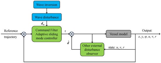
Figure 2.
Trajectory tracking control diagram of USV.
3.1. Design of the Nonlinear Disturbance Observer
A nonlinear disturbance observer is constructed based on vessel dynamics (2) as follows:
where represents the vector of perturbation estimates output by the observer. is a designed diagonal matrix with positive definite parameters, and is an intermediate auxiliary state vector.
To demonstrate the effectiveness of the designed perturbation observer, the perturbation observation error vector is defined as follows:
By taking the time derivative of Equation (12), and substituting Equations (2), (13) and (14), we obtain:
The Lyapunov function of the perturbed observer is defined as follows:
Based on Young’s inequality and considering Assumption 3, we can obtain:
where is a constant. Thus, we can rewrite Equation (18) as:
In this context, when the external disturbance is an unknown constant vector, the bound of the disturbance rate of change is . Consequently, it can be inferred that the observation error of the disturbance observer converges to 0.
Solving the inequality (20), we obtain:
where will ultimately be bounded and will converge within a spherical region centered at the origin with radius . Additionally, from Equation (14), we know that will converge within a spherical region centered at the origin with radius .
Under the condition specified in Equation (18), by appropriately choosing the parameters and , can be made arbitrarily small. This implies that the disturbance observer can estimate external disturbances and measurement errors with arbitrary precision.
3.2. Design of Command Filter Adaptive Sliding Model Controller
Define the position tracking error vector :
where is a vector consisting of the desired position and the yaw angle, and is the vector of the system’s position output. The system will track the desired position if .
Define the velocity error vector :
From Equation (2), we get:
By taking the time derivative of and using Equation (1), we obtain:
Design the virtual control vector for :
where is a positive definite parameter diagonal matrix of the design.
Let the virtual control pass through the following command filter:
where is the filtered virtual control vector, is the state vector of the command filter, and and are design parameters of the command filter. The initial conditions are .
The introduction of the command filter makes the system have a filtering error vector ,
To eliminate the filtering error , We introduce the compensated state vector, whose dynamic equations are designed as:
where is the compensated state vector with the initial condition .
Define the compensated tracking error vector as:
Since the wind and current perturbations and the wave perturbation calculation errors are unknown, the design control law to enhance the robustness of the system against external disturbances by combining the sliding mode design method is as follows:
where is designed as the sliding manifold, is the equivalent control input, and is the switching control input. , is the i-th component of , ; is the upper bound vector for the unknown external perturbation ; is the designed diagonal matrix of positive definite parameters; and is used to eliminate the coupling term.
To avoid the sliding mode chattering problem, the disturbance is estimated using the disturbance observer designed above, and the modified control law is:
The adaptive law is introduced to estimate the bounds of the perturbation observation error, and combined with the hyperbolic tangent function to further mitigate the sliding mode chattering in order to improve control accuracy. The optimized control law is:
where ; is a vector consisting of estimates of the upper bound of the unknown uncertainty term, and again the upper bound of the perturbation observation error .
We design the adaptive law with a modified leakage term with to estimate bounding vector of the perturbation observation error:
where is the designed positive definite parameter diagonal matrix; is the positive definite parameter diagonal matrix of the design, which is set to a very small value that guarantees does not grow to infinity; and is the prior estimate of , .
Theorem 1.
Consider the three-degree-of-freedom, fully driven ship engaged in trajectory-tracking, governed by the nonlinear kinematics and dynamics Equations (1) under Assumptions 1, 2, and 3. The design incorporates a nonlinear perturbation observer as per Equations (12) and (13) to estimate external environmental disturbances. Additionally, a command filter is formulated using Equation (28) to prevent derivative explosions, and a σ-corrected leakage term in the adaptive law, based on Equation (37), helps estimate the bounds of perturbation observation errors. The control strategy, detailed in Equation (36), utilizes design parameters , , ,
, , , and as specified in Equation (47). This design ensures the surface ship’s actual trajectory η closely follows the desired trajectory , achieving minimal tracking errors. Moreover, it guarantees that all signals within the closed-loop control system for trajectory tracking remain ultimately uniformly bounded (UUB).
3.3. Stability Proof
Selection of the Lyapunov function for the three-degree-of-freedom fully driven trajectory tracking vessel control system:
where is the adaptive law to estimate the error vector, and by taking the time derivative of Equation (28), we can obtain:
According to the property of the coordinate system transformation matrix J, we can obtain:
From Equation (37), we obtain:
By the properties of the hyperbolic tangent function, for , there is established, and , so we can obtain:
where . According to the definition and the Cauchy–Schwartz inequality , we get the transformed form:
Combining Equations (20) and (43)–(45), we obtain:
where
and , , , , and is the smallest eigenvalue of the matrix, while is the largest eigenvalue of the matrix.
Solving Equation (46), we have:
From Equation (49), it is established that is ultimately uniformly bounded (UUB). Consequently, as indicated by Equation (38), the variables , , , and are also UUB. Additionally, the bounded nature of , , and is confirmed. The boundedness of , as deduced from Equation (32), ensures that is similarly constrained. Correspondingly, from Equation (27) and the limits placed on , the virtual control function is confirmed to be bounded. Given that and are bounded, it follows that is also bounded. The boundedness of implies that the estimated remains within the defined limits. Therefore, is likewise bounded. With and being bounded, it follows that , too, is bounded. Therefore, all signals within the trajectory tracking closed-loop control system are confirmed to be ultimately uniformly bounded.
Due to the boundedness of , that is with being a positive constant, the Lyapunov function is defined as follows:
According to Equation (30) and Young’s inequality, we obtain:
where and
Solving Equation (51), we obtain:
Then, there is a constant such that, for any positive constant , we have for all . Therefore, the tracking error converges to a compact set . Thus, we can prove Theorem 1.
4. Simulation and Result Analysis
In order to demonstrate the effectiveness of our designed control strategy, we use a supply vessel as an experimental object, and the relevant parameters of the vessel are as follows [45]: the length of the vessel L is 76.2 m, the breadth is 20 m, and the draft is 5 m. The relevant parameters of the vessel model are as follows:
The total disturbances are divided into two parts: wave force disturbances and other external environmental disturbances that are difficult to compute directly. Next, we will introduce the simulation parameters for these disturbances.
The parameters related to wave force disturbances are set as follows: the speed of the USV, U, is assumed to be 10 m/s; the heading angle is set to 30 degrees; the wave direction angle is set to 45 degrees; and the density of seawater is 1025 kg/m3. The simulation results are shown in Figure 3, where Figure 3a demonstrates the time course profile of the wave force in the u-direction and Figure 3b demonstrates the time course profile of the wave moment in the r-direction.
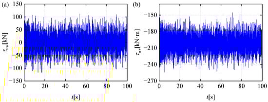
Figure 3.
Wave disturbance interference force: (a) is the interference force in the u-direction, and (b) is the disturbance torque in the r-direction.
Other external environmental perturbations are considered as the sum of wave inversion errors and wind, currents, and other external environmental perturbations that are difficult to calculate directly. For the former, the inversion error is considered to be 10%, and the latter is described by a first-order Markov process of the following form and parameter settings:
where represents the external environmental disturbances experienced by the ship in the inertial coordinate system, where is the wave-induced disturbance and is the error term from wave inversion; is the designed time constant diagonal matrix; is the zero-mean Gaussian noise vector; and is the covariance matrix of n.
The circle trajectory that is expected to be tracked is set as , the initial position and velocity information of the ship are , and the initial state information of the disturbance observer is . The controller parameters are , , , , , , , and , and the filter time constant is . Thus, when ∼ satisfy , , , the condition (47) holds.
Figure 4, Figure 5, Figure 6, Figure 7, Figure 8, Figure 9 and Figure 10 show the simulation results of the path-following model of this fully-driven supply vessel under the unmanned vessel path-following control strategy designed in Section 3. Figure 4 shows a comparison of (a) the straight line trajectory and (b) the circle trajectory tracking simulation curves before and after wave compensation. The results indicate that after wave compensation, both these two trajectories are tracked more quickly and with higher accuracy compared to before wave compensation. Figure 5 presents the time history curves and tracking errors for the vessel’s expected position, expected yaw angle, and actual position and yaw angle within the inertial coordinate system. The figure demonstrates that the spacecraft successfully tracks the desired trajectory within approximately 40 s, with the tracking errors in all three degrees of freedom ultimately converging to zero. Figure 6 illustrates the tracking performance of a circle trajectory. We also add the proportional-integral-derivative (PID) controller as a comparison, where our method has a better performance than PID controller during the whole controlling process obviously. The vertical coordinate, denoted as effect, is computed using the formula , where X and Y represent the reference trajectory coordinates, x and y denote the actual trajectory coordinates, signifies the actual direction, and t indicates time. This formula measures the Euclidean distance error between the actual and reference trajectories, encompassing both positional and directional discrepancies.
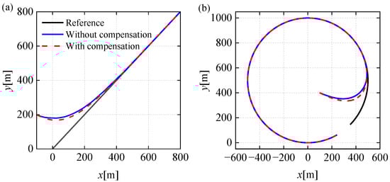
Figure 4.
Effect of trajectory tracking control with and without wave compensation for (a) straight line trajectory and (b) circle trajectory.
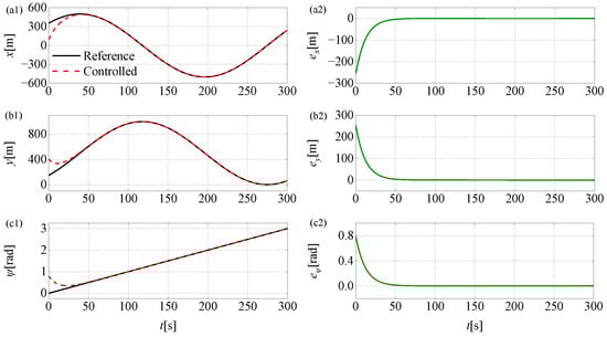
Figure 5.
Effectiveness and error of trajectory tracking. Subfigures (a1), (b1), and (c1) illustrate the tracking effectiveness in the x, y, and directions, respectively. Subfigures (a2), (b2), and (c2) show the corresponding tracking errors in the x, y, and directions.
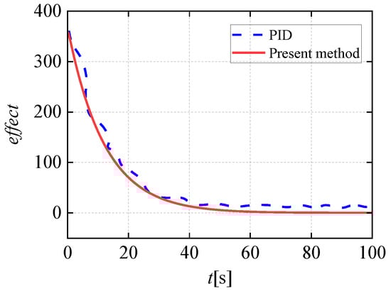
Figure 6.
A comparison for tracking performance of circle trajectory between the present method and the PID method.
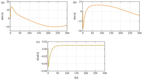
Figure 7.
Actual speed of unmanned vessels. Subfigure (a) shows the actual surge velocity u in the x direction. Subfigure (b) illustrates the sway velocity v in the y direction. Subfigure (c) displays the yaw rate r in the direction.
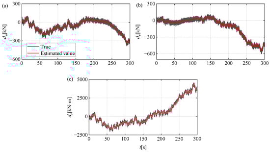
Figure 8.
Other external disturbances and observer estimates. Subfigure (a) corresponds to the x direction, (b) to the y direction, and (c) to the direction.
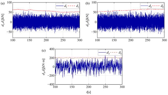
Figure 9.
Observation error and upper bound estimation for observers. Subfigure (a) shows the x direction, (b) the y direction, and (c) the direction.
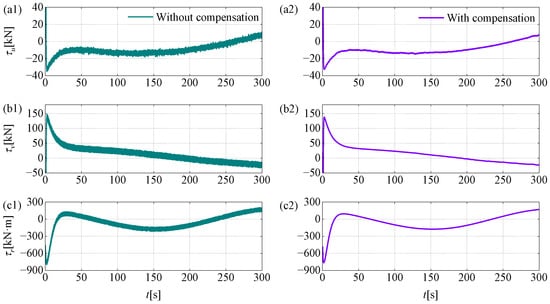
Figure 10.
Controller output before and after compensation. Subfigures (a1), (b1), and (c1) show the control outputs in the x, y, and directions without wave compensation, respectively. Subfigures (a2), (b2), and (c2) show the control outputs in the x, y, and directions with wave compensation, respectively.
Figure 7 displays the time history curves of the vessel’s actual surge velocity u, sway velocity v, and yaw rate r in the presence of additional external environmental perturbations d and actual wave disturbances . Figure 8 shows the time history curves of external environmental perturbations d affecting the vessel and the corresponding perturbations estimated by the perturbation observer. The results indicate that the designed perturbation observer effectively estimates external environmental perturbations that are challenging to measure directly.
Figure 9 illustrates the observation error and the upper bound of the perturbation observer. It is evident that the adaptive rate parameter, based on the -corrected leakage term, is appropriately selected, allowing for a more precise estimation of the perturbation observation error bound.
Figure 10 depicts the controller output time history curve, showing that the overall controller output remains smooth and reasonable after the perturbation observer compensates for perturbations and the adaptive law, combined with the hyperbolic tangent function, mitigates the perturbation observation error. It can be observed that the addition of wave feedforward compensation further reduces controller output jitter, highlighting the efficacy of wave feedforward compensation in diminishing jitter phenomena.
5. Conclusions
This paper investigates the trajectory tracking control problem of USVs based on real-time wave disturbance compensation. Firstly, based on previous work, wave information from the actual sea surface is extracted through stereoscopic visual observations, and data preprocessing is performed using a task-driven point cloud downsampling network. Then, the phase-resolved wave field is reconstructed in real time. Subsequently, the wave disturbances are mechanically modeled, and real-time wave disturbances are used as feedforward inputs. Furthermore, a backstepping sliding mode control law is designed. This control law employs command filters to avoid the differential explosion problem and uses a hyperbolic tangent function to mitigate sliding mode chattering. An adaptive law is also designed to estimate and compensate for other external disturbances and the upper bounds of inversion errors that cannot be computed in real time. Simulation results show that, with appropriate control parameter selection, the proposed control strategy has good trajectory tracking performance, and the controller output is relatively smooth, demonstrating the effectiveness of the proposed control strategy.
This method directly acquires real wave disturbance data from the time domain, bringing potential advancements to the field of wave-aware control. Future research could further explore multi-sensor fusion technologies and perception-based advanced control algorithms to promote intelligent development in marine engineering. Additionally, incorporating machine learning and artificial intelligence technologies to optimize the adaptive capabilities and real-time performance of control strategies will provide new solutions for the applications of USVs and other autonomous maritime equipment.
Author Contributions
T.M.: Conceptualization (lead); formal analysis (lead); investigation (lead); methodology (lead); validation (lead); visualization (lead); writing—original draft (lead); writing—review and editing (equal). Z.S.: supervision (lead); writing—review and editing (equal). Z.Z.: writing—review and editing (equal). All authors have read and agreed to the published version of the manuscript.
Funding
This work is supported by the National Natural Science Foundation of China (No. 51879027).
Data Availability Statement
Data are contained within the article.
Conflicts of Interest
The authors report no conflicts of interest.
Appendix A
Phase-Resolved Wave Fields Reconstruction by Task-Driven Learning Downsampling Network
The aim of this study is to select an optimal subset from the comprehensive point cloud . This selection is critical for improving the efficacy of subsequent wave reconstruction tasks denoted by T. The selection process is formulated as an optimization challenge:
with indicative of the point cloud’s variability during training phases. To tackle this optimization, a streamlined network approach utilizing multilayer perceptrons (MLP) is implemented. The task-specific loss aims to reduce the reconstruction error as defined by:
where stands for the completeness ratio, which assesses the fidelity of the 3D wave reconstruction. This metric is calculated by:
and N denotes the total count of points in the processed point cloud, with being contingent upon . For each corresponding point, the residual’s absolute magnitude is:
where and respectively represent the true wave elevation and the reconstructed wave height, using the phase-resolved wave reconstruction technique discussed subsequently. The coverage points meeting the threshold are then used to compute the coverage rate, with the threshold defined as .
For the inversion and reconstruction of the phase-resolved wave fields using sampled points , the study applies the linear wave theory (LWT) based on the Eulerian framework, which is suited for modeling non-viscous, non-cohesive, and irrotational fluids. In a Cartesian coordinate system , with horizontal orientation for x and y axes and vertical alignment for z axis, the superposition of wave harmonics characterized by amplitude , angular frequency , and propagation direction is used to depict the ocean surface in the horizontal plane:
where t represents time; consists of random phases, with being uniformly distributed random numbers; and and describe the wave vectors and wavenumbers, respectively. Utilizing the deep water dispersion relationship, wavenumbers are derived from , where g is the gravitational acceleration.
where are wave harmonic parameters describing the ocean surface, while and are spatio-temporal phases.
Using a linear wave model, we perform the inversion of wave parameters for reconstructing the sea surface. The prevalent method for reconstructing waves from observed data utilizes a variational approach. This method optimizes the parameters to minimize the root-mean-square (RMS) discrepancy between the observed wave data and the model’s output. Therefore, the cost function is formulated as:
where denotes the vector of unknown parameters, is the modeled sea surface elevation, and represents the point cloud elevations from sampled observations.
To determine these model parameters, the cost function is minimized, yielding the following system of equations:
where .
This results in a linear system of equations for the unknowns:
where represents the harmonic phases of the waves.
These equations are reformulated in a matrix form as:
where encapsulates the unknown parameters , and A is the matrix defined by:
and B is the vector:
In cases with short-peak waves, the condition number of matrix A often becomes large, leading to potential issues with inversion. To mitigate this, Tikhonov regularization is applied, optimizing an adjusted error function:
with chosen through generalized cross-validation (GCV) to ensure reliability in the observations. The optimal regularization parameter corresponds to the minimal value of the GCV function. After determining the wave parameters, the phase-resolved wave field is reconstructed, which is crucial for computing the task loss as per Equation (A4).
Figure A1 illustrates the comparison between actual and reconstructed ocean waves, showcasing the effectiveness of the variational method in reproducing waves with minimal discrepancies, thus serving as reliable inputs for further processing.

Figure A1.
Comparison of actual and reconstructed waves: (a) actual wave, and (b) reconstructed wave.
Figure A1.
Comparison of actual and reconstructed waves: (a) actual wave, and (b) reconstructed wave.

References
- Mahacek, P.; Kitts, C.A.; Mas, I. Dynamic guarding of marine assets through cluster control of automated surface vessel fleets. IEEE/ASME Trans. Mechatron. 2011, 17, 65–75. [Google Scholar] [CrossRef]
- Liu, Z.; Zhang, Y.; Yu, X.; Yuan, C. Unmanned surface vehicles: An overview of developments and challenges. Annu. Rev. Control 2016, 41, 71–93. [Google Scholar] [CrossRef]
- Jiang, H.K.; Luo, K.; Zhang, Z.Y.; Wu, J.; Yi, H.L. Global linear instability analysis of thermal convective flow using the linearized lattice Boltzmann method. J. Fluid Mech. 2022, 944, A31. [Google Scholar] [CrossRef]
- Barrera, C.; Padron, I.; Luis, F.; Llinas, O. Trends and challenges in unmanned surface vehicles (Usv): From survey to shipping. TransNav Int. J. Mar. Navig. Saf. Sea Transp. 2021, 15, 135–142. [Google Scholar] [CrossRef]
- Du, B.; Lin, B.; Zhang, C.; Dong, B.; Zhang, W. Safe deep reinforcement learning-based adaptive control for USV interception mission. Ocean Eng. 2022, 246, 110477. [Google Scholar] [CrossRef]
- Peng, Z.; Liu, E.; Pan, C.; Wang, H.; Wang, D.; Liu, L. Model-based deep reinforcement learning for data-driven motion control of an under-actuated unmanned surface vehicle: Path following and trajectory tracking. J. Frankl. Inst. 2023, 360, 4399–4426. [Google Scholar] [CrossRef]
- Lin, M.; Zhang, Z.; Pang, Y.; Lin, H.; Ji, Q. Underactuated USV path following mechanism based on the cascade method. Sci. Rep. 2022, 12, 1461. [Google Scholar] [CrossRef] [PubMed]
- Yu, J.; Chen, Y.; Yang, M.; Chen, Z.; Xu, J.; Lu, Y.; Zhao, Z. A path planning algorithm for unmanned surface vessel with pose constraints in an unknown environment. Int. J. Nav. Archit. Ocean. Eng. 2024, 16, 100602. [Google Scholar] [CrossRef]
- Liu, Z.; Zhang, Y.; Yuan, C.; Luo, J. Adaptive path following control of unmanned surface vehicles considering environmental disturbances and system constraints. IEEE Trans. Syst. Man. Cybern. Syst. 2018, 51, 339–353. [Google Scholar] [CrossRef]
- Gonzalez-Garcia, A.; Castañeda, H. Adaptive integral terminal sliding mode control for an unmanned surface vehicle against external disturbances. IFAC-PapersOnLine 2021, 54, 202–207. [Google Scholar] [CrossRef]
- Walker, K.L.; Gabl, R.; Aracri, S.; Cao, Y.; Stokes, A.A.; Kiprakis, A.; Giorgio-Serchi, F. Experimental validation of wave induced disturbances for predictive station keeping of a remotely operated vehicle. IEEE Robot. Autom. Lett. 2021, 6, 5421–5428. [Google Scholar] [CrossRef]
- Clauss, G.F.; Stutz, K. Time-domain analysis of floating bodies with forward speed. J. Offshore Mech. Arct. Eng. 2002, 124, 66–73. [Google Scholar] [CrossRef][Green Version]
- Fu, M.; Wang, L. Adaptive finite-time event-triggered control of marine surface vehicles with prescribed performance and output constraints. Ocean Eng. 2021, 238, 109712. [Google Scholar] [CrossRef]
- Xu, J.; Cui, Y.; Xing, W.; Huang, F.; Yan, Z.; Wu, D.; Chen, T. Anti-disturbance fault-tolerant formation containment control for multiple autonomous underwater vehicles with actuator faults. Ocean Eng. 2022, 266, 112924. [Google Scholar] [CrossRef]
- Jiang, H.; Cao, S. Balanced proper-orthogonal-decomposition-based feedback control of vortex-induced vibration. Phys. Rev. Fluids 2024, 9, 073901. [Google Scholar] [CrossRef]
- Lu, Y.; Zhang, G.; Sun, Z.; Zhang, W. Adaptive cooperative formation control of autonomous surface vessels with uncertain dynamics and external disturbances. Ocean Eng. 2018, 167, 36–44. [Google Scholar] [CrossRef]
- Mou, T.; Shen, Z.; Xue, G. Task-Driven Learning Downsampling Network Based Phase-Resolved Wave Fields Reconstruction with Remote Optical Observations. J. Mar. Sci. Eng. 2024, 12, 1082. [Google Scholar] [CrossRef]
- Zhang, G.; Chu, S.; Zhang, W.; Liu, C. Adaptive neural fault-tolerant control for USV with the output-based triggering approach. IEEE Trans. Veh. Technol. 2022, 71, 6948–6957. [Google Scholar] [CrossRef]
- Jiang, H.K.; Zhang, Y.; Zhang, Z.Y.; Luo, K.; Yi, H.L. Instability and bifurcations of electro-thermo-convection in a tilted square cavity filled with dielectric liquid. Phys. Fluids 2022, 34, 064116. [Google Scholar] [CrossRef]
- Er, M.J.; Gao, W.; Li, Q.; Li, L.; Liu, T. Composite trajectory tracking of a ship-borne manipulator system based on full-order terminal sliding mode control under external disturbances and model uncertainties. Ocean Eng. 2023, 267, 113203. [Google Scholar] [CrossRef]
- Zhao, Y.; Qi, X.; Ma, Y.; Li, Z.; Malekian, R.; Sotelo, M.A. Path following optimization for an underactuated USV using smoothly-convergent deep reinforcement learning. IEEE Trans. Intell. Transp. Syst. 2020, 22, 6208–6220. [Google Scholar] [CrossRef]
- Liu, Z.Q.; Wang, Y.L.; Han, Q.L. Adaptive fault-tolerant trajectory tracking control of twin-propeller non-rudder unmanned surface vehicles. Ocean Eng. 2023, 285, 115294. [Google Scholar] [CrossRef]
- Zhang, J.X.; Yang, T.; Chai, T. Neural network control of underactuated surface vehicles with prescribed trajectory tracking performance. IEEE Trans. Neural Netw. Learn. Syst. 2022, 35, 8026–8039. [Google Scholar] [CrossRef] [PubMed]
- Wang, N.; Gao, Y.; Zhao, H.; Ahn, C.K. Reinforcement learning-based optimal tracking control of an unknown unmanned surface vehicle. IEEE Trans. Neural Netw. Learn. Syst. 2020, 32, 3034–3045. [Google Scholar] [CrossRef] [PubMed]
- Vaidyanathan, S.; Azar, A.T. Backstepping Control of Nonlinear Dynamical Systems; Academic Press: Cambridge, MA, USA, 2020. [Google Scholar]
- Liao, Y.L.; Wan, L.; Zhuang, J.Y. Backstepping dynamical sliding mode control method for the path following of the underactuated surface vessel. Procedia Eng. 2011, 15, 256–263. [Google Scholar] [CrossRef]
- Zhao, Y.; Sun, X.; Wang, G.; Fan, Y. Adaptive backstepping sliding mode tracking control for underactuated unmanned surface vehicle with disturbances and input saturation. IEEE Access 2020, 9, 1304–1312. [Google Scholar] [CrossRef]
- Li, M.; Guo, C.; Yuan, Y.; Guo, M. Path following control of the asymmetric USV via backsteppin sliding mode technique. In Proceedings of the 2019 Chinese Control and Decision Conference (CCDC), Nanchang, China, 3–5 June 2019; pp. 2979–2984. [Google Scholar]
- Chen, J.; Zhang, Q.; Qi, Y.; Leng, Z.; Zhang, D.; Xie, J. Trajectory Tracking Based on Backstepping Sliding Mode Control for Underactuated USV. In Proceedings of the 2021 36th Youth Academic Annual Conference of Chinese Association of Automation (YAC), Nanchang, China, 28–30 May 2021; pp. 294–299. [Google Scholar]
- Dong, J.; Zhao, M.; Cheng, M.; Wang, Y. Integral terminal sliding-mode integral backstepping adaptive control for trajectory tracking of unmanned surface vehicle. Cyber-Phys. Syst. 2023, 9, 77–96. [Google Scholar] [CrossRef]
- Xue, G.; Lin, F.; Li, S.; Liu, H. Adaptive fuzzy finite-time backstepping control of fractional-order nonlinear systems with actuator faults via command-filtering and sliding mode technique. Inf. Sci. 2022, 600, 189–208. [Google Scholar] [CrossRef]
- Shtessel, Y.; Edwards, C.; Fridman, L.; Levant, A. Sliding Mode Control and Observation; Springer: Berlin/Heidelberg, Germany, 2014; Volume 10. [Google Scholar]
- Paravisi, M.; Santos, D.H.; Jorge, V.; Heck, G.; Gonçalves, L.M.; Amory, A. Unmanned surface vehicle simulator with realistic environmental disturbances. Sensors 2019, 19, 1068. [Google Scholar] [CrossRef]
- Wei, H.; Shen, C.; Shi, Y. Distributed Lyapunov-based model predictive formation tracking control for autonomous underwater vehicles subject to disturbances. IEEE Trans. Syst. Man. Cybern. Syst. 2019, 51, 5198–5208. [Google Scholar] [CrossRef]
- Chen, Z.; Zhang, Y.; Zhang, Y.; Nie, Y.; Tang, J.; Zhu, S. Disturbance-observer-based sliding mode control design for nonlinear unmanned surface vessel with uncertainties. IEEE Access 2019, 7, 148522–148530. [Google Scholar] [CrossRef]
- Wang, N.; Sun, Z.; Yin, J.; Su, S.F.; Sharma, S. Finite-time observer based guidance and control of underactuated surface vehicles with unknown sideslip angles and disturbances. IEEE Access 2018, 6, 14059–14070. [Google Scholar] [CrossRef]
- Huang, C.; Zhang, X.; Zhang, G. Improved decentralized finite-time formation control of underactuated USVs via a novel disturbance observer. Ocean Eng. 2019, 174, 117–124. [Google Scholar] [CrossRef]
- Zhang, Y.; Chen, Z.; Nie, Y.; Tang, J.; Zhu, S. Adaptive Sliding Mode Control Design for Nonlinear Unmanned Surface Vessel With Fuzzy Logic System and Disturbance-Observer. In Proceedings of the 2020 IEEE/ASME International Conference on Advanced Intelligent Mechatronics (AIM), Boston, MA, USA, 6–9 July 2020; pp. 1298–1303. [Google Scholar]
- Feng, N.; Wu, D.; Yu, H.; Yamashita, A.S.; Huang, Y. Predictive compensator based event-triggered model predictive control with nonlinear disturbance observer for unmanned surface vehicle under cyber-attacks. Ocean Eng. 2022, 259, 111868. [Google Scholar] [CrossRef]
- Mu, D.; Li, J.; Wang, G.; Fan, Y. Research on path following control of unmanned ship based on fast wave inversion disturbance compensation and preset performance. Ocean Eng. 2024, 304, 117864. [Google Scholar] [CrossRef]
- Mu, D.; Li, J.; Wang, G.; Fan, Y. Disturbance rejection control of adaptive integral LOS unmanned ship path following based on fast wave inversion. Appl. Ocean. Res. 2024, 144, 103907. [Google Scholar] [CrossRef]
- Fossen, T.I. Handbook of Marine Craft Hydrodynamics and Motion Control; John Wiley & Sons: Hoboken, NJ, USA, 2011. [Google Scholar]
- Nielsen, U.D. Estimations of on-site directional wave spectra from measured ship responses. Mar. Struct. 2006, 19, 33–69. [Google Scholar] [CrossRef]
- Mu, D.; Lang, Z.; Fan, Y.; Zhao, Y. Time-varying encounter angle trajectory tracking control of unmanned surface vehicle based on wave modeling. ISA Trans. 2023, 142, 409–419. [Google Scholar] [CrossRef]
- Fossen, T.I.; Sagatun, S.I.; Sørensen, A.J. Identification of dynamically positioned ships. Control. Eng. Pract. 1996, 4, 369–376. [Google Scholar] [CrossRef]


Disclaimer/Publisher’s Note: The statements, opinions and data contained in all publications are solely those of the individual author(s) and contributor(s) and not of MDPI and/or the editor(s). MDPI and/or the editor(s) disclaim responsibility for any injury to people or property resulting from any ideas, methods, instructions or products referred to in the content. |
© 2024 by the authors. Licensee MDPI, Basel, Switzerland. This article is an open access article distributed under the terms and conditions of the Creative Commons Attribution (CC BY) license (https://creativecommons.org/licenses/by/4.0/).