Abstract
The Automatic Identification System (AIS) utilizes base stations to manage vessel traffic and disseminate waterway information. These stations broadcast maritime safety data to vessels within their service radius using VHF signals. However, the emergence of “spoofing base stations” poses a significant threat to maritime safety. These impostors mimic legitimate AIS base stations by appropriating their Maritime Mobile Service Identity (MMSI) information, interacting with vessels, potentially leading to erroneous decisions, or guiding vessels into hazardous areas. Therefore, ensuring the credibility of AIS base stations is critical for safe vessel navigation. It is essential to distinguish between genuine AIS base stations and “spoofing base stations” to achieve this goal. One criterion for identifying AIS spoofing involves detecting signals beyond the expected service radius of AIS base stations. This paper proposes a method to monitor the credibility of AIS base stations through a service radius detection pattern. Furthermore, the method analyzes the impact of hydrological and meteorological factors on AIS signal propagation in complex sea surface environments. By integrating empirical data, it accurately describes the mathematical relationship and calculates the service radius of AIS base station signals. Analyzing vessel position coordinates, decoding base station position messages, and computing distances between vessels and AIS base stations allows for matching with the AIS base station’s designated service radius and propagation distance. This approach enables precise identification of AIS spoofing base stations, thereby facilitating robust monitoring of AIS base station credibility. The research outcomes provide a foundational framework for developing high-credibility AIS base station services within integrated maritime navigation and information systems.
1. Introduction
The Automatic Identification System (AIS) is a mandatory navigation system pre-scribed by the SOLAS Convention for equipping ships. It serves the purpose of facilitating automatic identification and information exchange not only between ships but also be-tween ships and base stations. Presently, the AIS stands as the principal system for enhancing navigation and averting collisions at sea. It oversees ship navigation safety by means of a network of AIS base stations that vigilantly monitor maritime traffic. Consequently, the AIS not only enhances the efficiency of ship navigation but also fortifies transportation safety.
As a critical element of AIS, AIS base stations fulfill essential roles such as vessel monitoring, distress alert reception, coordination of vessel activities, and traffic management. However, these stations are vulnerable to potential attacks from AIS “spoofing base stations” that hijack the MMSI identity of legitimate AIS bases. Using this stolen identity, spoofing stations communicate false navigational data within their service radius [1]. This misinformation can lead to erroneous decisions by vessel crews, increasing collision risks, directing ships into hazardous zones, or guiding them toward illicit activities. Thus, effective technical measures and management strategies are necessary to promptly detect and mitigate threats like AIS identity spoofing, ensuring the authenticity and credibility of AIS broadcasted information.
Currently, research on AIS base station credibility typically involves anomaly detection within the AIS system and assessing the credibility of AIS data. Zhang et al. studied the Shanghai Port, developing an automatic detection method for base station-type navigational links to maintain network system integrity [2]. Cao et al. focused on the Yangtze River channel, conducting quality assessments of AIS base station virtual navigational aids to bolster credibility [3]. Wu et al. engineered a secure AIS system leveraging 5G networks and AI to detect malicious attacks and radio interference [4]. Specht et al. addressed uncovered coastal AIS areas hindering business continuity by devising a model for simulating vessel trajectories and detecting system faults through integrity monitoring [5]. Handani et al. integrated multiple remote base stations into a unified AIS monitoring system via a secure Internet-connected VPN, ensuring robust AIS data transmission security [6].
Regarding the credibility of AIS data, the AIS system operates as an open broadcast system where all ships and base stations publicly transmit message formats and content [7]. Attackers can exploit identity spoofing to impersonate legitimate entities and broadcast forged information, thereby disseminating false data or disrupting communications between vessels and base stations. To enhance AIS data quality and facilitate real-time analysis, Zhang et al. introduced a real-time algorithm for AIS data cleaning and metric analysis. Their approach incorporates techniques like linear regression and multi-trajectory tracking to rectify abnormal AIS data, thereby improving data quality and resolving issues related to vessel trajectory anomalies [8]. Shyshkin et al. addressed potential network attacks on AIS operations, such as false distress or safety messages and threats from fabricated virtual navigational devices. They proposed a method leveraging message authentication code schemes and digital watermarking technology to ensure the authenticity and integrity of AIS messages. Research findings indicate that this method seamlessly integrates with existing AIS functionalities [9]. Le Roy et al. proposed a solution that incorporates the Time Division Multiple Access (TDMA) communication protocol to mitigate issues with AIS forged data and the concealment of illicit activities. Their approach verifies message compliance with system-defined protocol standards to effectively detect abnormal messages [10]. Willett et al. focused on the deliberate reporting of false position information in AIS message reports, which can cause vessels to deviate from intended routes. They identified AIS abnormal data through kinematic analysis of vessel trajectories [11]. Soares et al. automated the grouping of AIS data based on features such as vessel type, size, and final destination within AIS message data. They employed trajectory compression and clustering algorithms to detect anomalies in AIS data [12]. Chen et al. proposed an AIS data anomaly detection method based on AIS trajectories, utilizing the K-means clustering method to identify abnormal data [13].
In conclusion, after reviewing existing research on anomaly monitoring in the AIS system and assessing the credibility of AIS data, it is evident that there is a significant gap in addressing uncredible AIS base station services due to “spoofing base stations”. These fraudulent stations usurp the MMSI of legitimate ones, communicating with vessels both within and beyond the genuine stations’ coverage areas through identity spoofing. Therefore, ensuring the integrity of data exchanges between AIS base stations and vessels requires vigilant monitoring of AIS base station credibility. To address this issue, this paper proposes a method for monitoring AIS base station credibility based on service radius detection patterns in the complex sea surface environment. This approach quantifies signal transmission loss from AIS base stations to accurately determine their signal coverage radius. By decoding vessel position coordinates and base station location information, the method calculates the distance between the AIS base station and the vessel. Subsequently, it employs matching analysis between this distance and the AIS base station’s signal service radius to effectively identify identity-spoofing AIS base stations.
2. The Influence of Various Marine Environmental Factors on the Signal Service Radius of AIS Base Stations
The AIS base station signal operates within the VHF band, and in the VHF communication system, the link budget is assessed using Equations (1)–(3). In Equation (1), SM represents the system margin, which signifies the variance between the received signal power and the sensitivity of the receiver equipment during signal transmission. A positive system margin (SM > 0) indicates that the signal power surpasses the receiver’s sensitivity, ensuring an ample energy reserve to counteract attenuation and interference. This reserve guarantees reliable demodulation and accurate data transmission at the receiving end [14]. Conversely, if the difference between the total system gain and loss is less than 0, the received signal power is insufficient, resulting in a decrease in signal communication quality or even abnormal communication. In essence, normal communication occurs only when the difference in Equation (1) is greater than 0. As the system margin diminishes with an increasing transmission distance, the maximum transmission distance at which the system margin remains positive defines the maximum service radius of the AIS base station signal.
The formula for calculating the margin of the maritime VHF communication system is:
where is the total system gain, and is the total system loss. The total system gain is determined as follows:
where is the transmit power, is the transmit antenna gain, is the receive antenna gain, and is the minimum protection power level required by the receiver.
The total system loss, thus calculated, is given by
where is the propagation path loss (dB), is the noise environment loss (dB) typically set to 5.5 dB for a typical port, is the transmitter feeder loss (dB), and is the receiver feeder loss (dB).
From Equations (1)–(3), it is evident that the service radius of the AIS base station signal is influenced by both the total system transmission loss and total system gain. The Standard outlines parameters, including transmit power, transmit antenna gain, receive antenna gain, transmitter feeder loss, and receiver feeder loss, as well as other related specifications [15]. According to the Standard, the AIS transmitter operates at 12.5 watts, has an antenna gain of 6 dBi or higher, and has a feeder loss of no more than 3 dB [15]. Additionally, the receiver sensitivity is −107 dBm (). Consequently, determining the transmission loss parameter () for the entire system is pivotal in calculating the signal coverage of the AIS base station. The relationship between the AIS base station signal transmission loss and the transmission distance is defined as follows:
where represents the transmission loss of AIS base station signals in a complex sea surface environment, denotes the environmental factor vector, represents various parameters describing the environmental factors, and represents the transmission distance of the AIS base station signal. A denotes the total system gain and any additional losses, with the exception of transmission path loss, expressed as:
When the system margin is zero, the transmission distance corresponding to is the service radius of the AIS base station.
The comprehensive analysis indicates that environmental noise loss (), transmitter feeder loss (), and receiver feeder loss () can be obtained by referencing the GB/T 39620 standard [15], which pertains to both the total system gain () and total system loss (). Therefore, the service radius of an AIS base station signal primarily depends on the transmission loss of the AIS base station signal. Since the electromagnetic propagation environment in maritime settings is influenced by several time-varying factors, such as sea conditions (tides, waves, etc.) and atmospheric conditions (temperature, wind speed, etc.), this study investigates the effects of sea surface wind speed, tidal effects, and evaporation duct on the service radius of AIS base station signals.
2.1. The Impact of Sea Surface Wind Speed on the Service Radius of AIS Base Station Signals
The sea surface becomes rougher as wind speeds increase [16]. Wind speed is the primary factor that drives wave formation and influences wave characteristics. Generally, higher wind speeds lead to more pronounced and vigorous wave fluctuations. When the AIS base station signal reflects off the wave surface, the variation in wave height modifies the signal reflection surface. Consequently, this induces changes in the signal propagation path, resulting in signal multipath and shadow effects [17], which subsequently impact the AIS signal reflection transmission loss.
The actual wave motion is a complex, three-dimensional random process. The simulation results of the three-dimensional random wave double superposition model are in good agreement with the measured results, and the accuracy of the model has been verified [18], which can apply to a wide range of applications in wind waves at different growth stages. Therefore, this study uses the three-dimensional wave double superposition model to perform the calculations. The expression of the 3D wave double superposition model is
where is the number of frequency divisions, is the number of directional divisions, is the number of waves, is the phase angle, is the random wave amplitude, and is defined as follows:
where is the frequency division interval, is the angular separation interval, and is defined as follows:
where is the spectral function of the wave, is the directional function of the wave, is the angular frequency of the wave, and is the random phase in [0, 2π].
In this paper, the PM spectrum is used as a spectral function for random wave generation, and the PM spectrum is expressed as
where and are constants taking the value = 0.008 and = 0.74, respectively, is the acceleration of gravity, is the wind speed at 19.5 m above the sea level, and is the angular frequency of the waves.
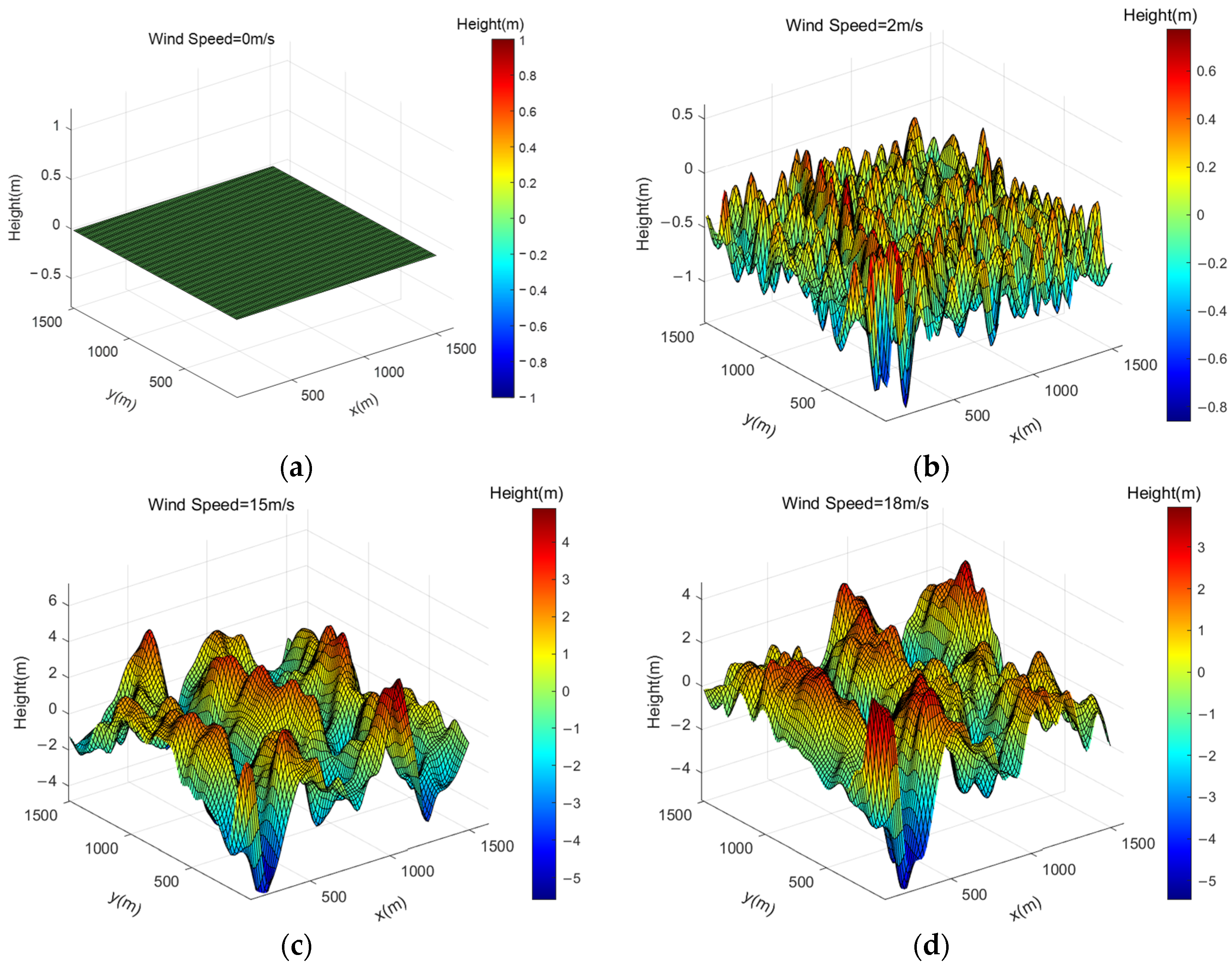
The wave models corresponding to wind speeds of 0 m/s, 2 m/s, 15 m/s, and 18 m/s are illustrated in Figure 1. Simulation results indicate that an increase in wind speed leads to more pronounced wave steepness, greater undulation, and increased wave amplitude. As the wave height increases, there are changes in the reflection path length of the AIS base station signal, which affects the received signal strength of AIS [19].
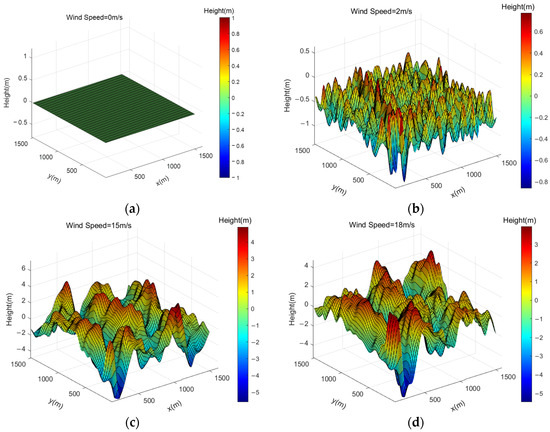
Figure 1.
Wave modeling at different wind speeds. (a) Wind Speed = 0 m/s; (b) Wind Speed = 2 m/s; (c) Wind Speed = 15 m/s; (d) Wind Speed = 18 m/s.
The reflection coefficient of the smooth sea surface can be calculated from the Fresnel reflection coefficient, which is divided into the horizontal polarization reflection coefficient and the vertical polarization reflection coefficient. Given that the AIS base station signal employs vertical polarization, the reflection coefficient of the AIS base station signal on a smooth sea surface is expressed as follows:
where is the relative permittivity of seawater, is the conductivity of seawater in S/m, is the wavelength of the AIS signal, and is the grazing angle of the AIS signal. The seawater’s relative permittivity and conductivity are affected by its temperature and salinity [20], which can be calculated by the Debye formula.
The reflection coefficient of the rough sea surface is the product of the reflection coefficient of the smooth sea surface and the roughness correction parameter, which is expressed as follows:
where is the modified Bessel function of the first kind with zero-order, is the sea surface roughness correction factor, and can be calculated from Equation (12):
where is the standard deviation of the wave height, is the wavelength of the AIS base station signal, and is the incident angle.
The standard deviation of the wave height can be calculated from the sea surface wind speed:
where is the wind speed at 10 m above sea surface.
The reflection coefficient of the rough sea surface is
where is the rough sea surface reflection coefficient, and is the modified Bessel function of the first kind with zero-order.
As sea surface wind speed increases, the sea becomes more turbulent and rough. Consequently, sea surface wind speed primarily affects the transmission loss of AIS base station reflected signals through changes in the sea surface reflection coefficient. When considering sea surface wind speed, the wireless channel model for AIS base station signals is as follows:
where and are the horizontal distances from the transmitter to the reflection point and from the receiver to the reflection point, respectively. is the transmitted electric field intensity, is the reflection coefficient, and is the speed of light.
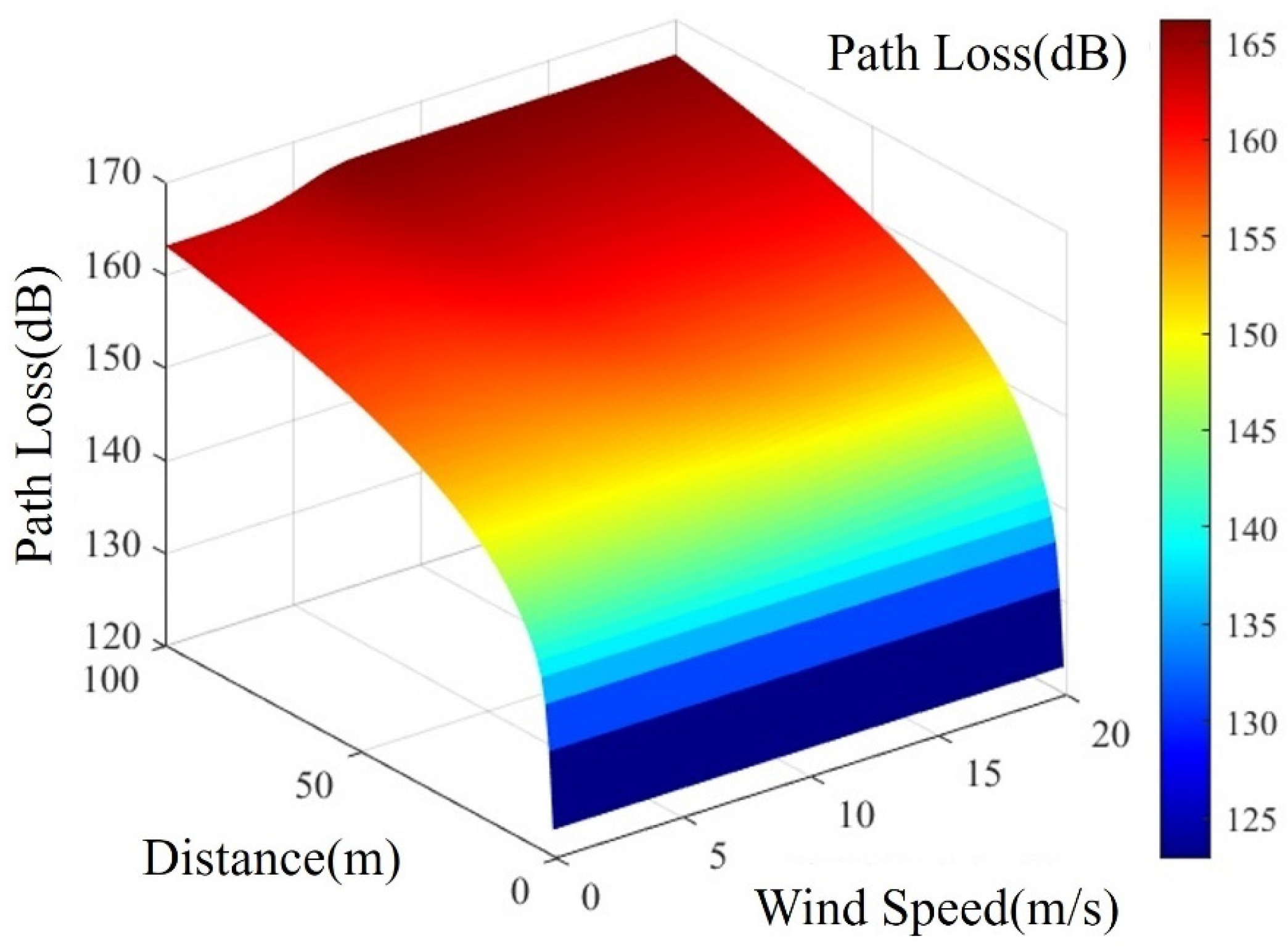
The transmission loss of VHF signals under different sea surface wind speeds is calculated using Equation (15) and depicted in Figure 2. Within a propagation distance of 5 km for VHF signals, transmission loss values hover around 140.1828 dB. This is primarily because the multipath propagation has relatively little effect on the signals within the 5 km transmission range. Additionally, the difference in signal paths from the transmitter to the receiver is relatively small in short-distance propagation. Consequently, this results in a reduced phase difference caused by the multipath propagation, leading to diminished interference effects between signals and contributing to signal stability.

Figure 2.
AIS Base Station Signal Transmission Loss under the Influence of Different Wind Speeds.
Beyond a 5 km transmission distance for AIS base station signals, the impact of rough sea surfaces becomes more pronounced under varying wind speed conditions. As transmission distance increases, higher wind speeds elevate sea surface roughness, amplifying electromagnetic wave reflection during propagation and thereby increasing propagation loss. This phenomenon underscores the critical role of sea conditions in long-distance AIS signal transmission, necessitating careful consideration and evaluation for accurate information delivery.
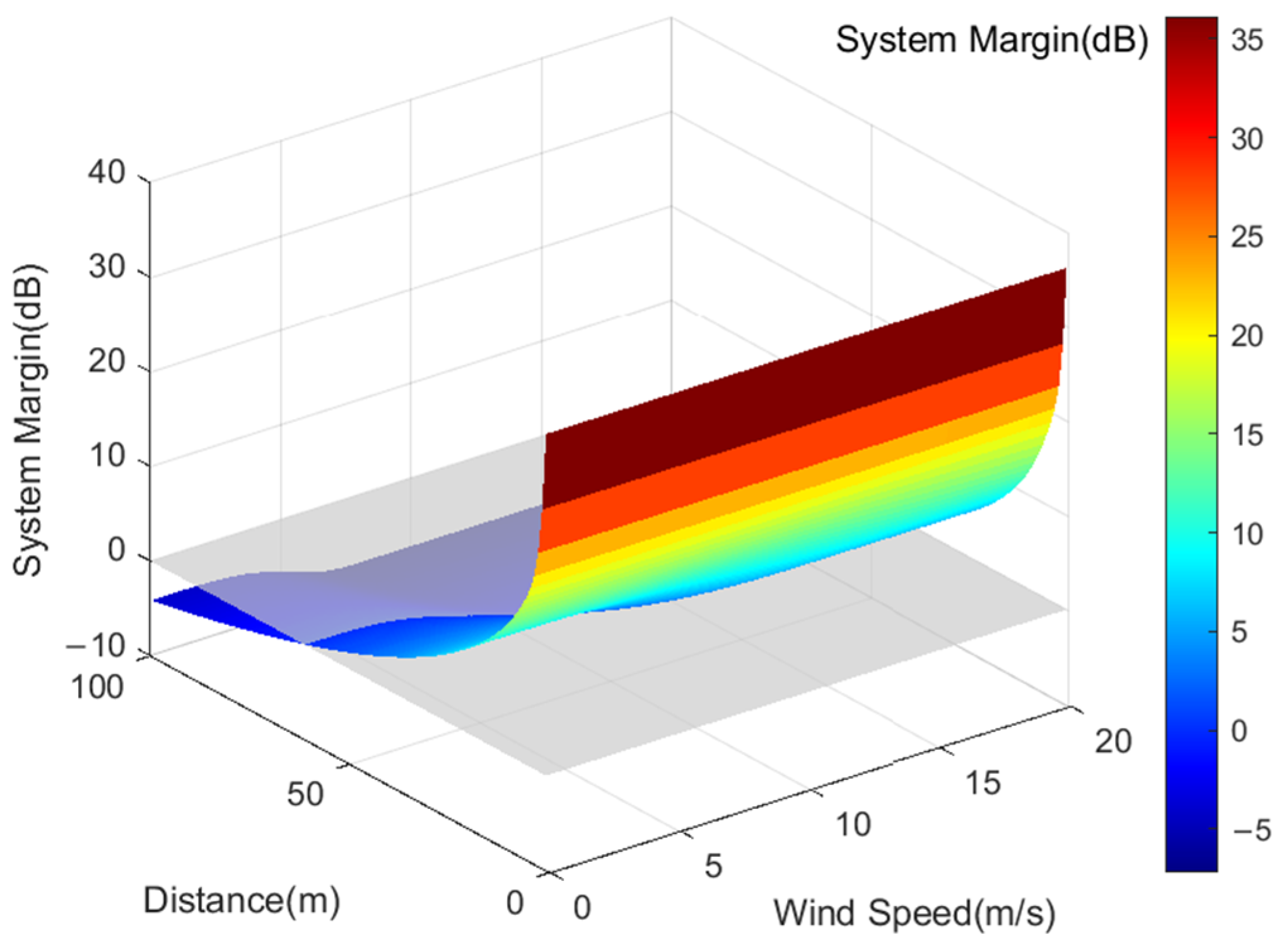
Moreover, the margin of the VHF system under different sea surface wind speeds can be determined by calculating VHF signal transmission losses, as illustrated in Figure 3. The system margin of VHF signals decreases with increasing transmission distance. For identical transmission distances, higher wind speeds yield smaller system margins for AIS base station signals. As wind speed escalates from 0 m/s to 18 m/s, the coverage range of VHF signals declines from 61 km to 43 km, reflecting a variance of 18 km. This reduction occurs because heightened wind speeds correspond to increased sea surface roughness, typically characterized by higher sea state levels. On rough sea surfaces, signals encounter more obstacles and sources of reflection, intensifying signal attenuation and consequently restricting the transmission range of VHF signals.

Figure 3.
AIS Base Station Signal Coverage under the Influence of Different Wind Speeds.
2.2. The Impact of Tidal Effects on the Service Radius of AIS Base Station Signals
The tidal effect results in periodic changes in ocean water levels, consequently modifying the geometry of the link between the reflected and direct paths of the AIS base station signal, as illustrated in Figure 4. Furthermore, the tidal effect impacts the height of the shipboard transceiver antenna as well as the angle of incidence [20], thereby influencing the quality of the received AIS signal.
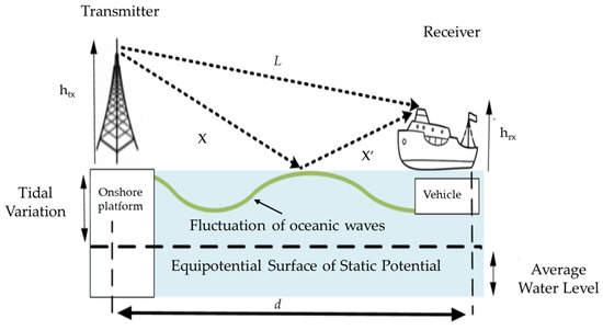
Figure 4.
Model the propagation of AIS base station signals under changing tidal water levels.
Since the tidal phenomenon impacts the transmission loss of AIS base station signals by changing the reflection path length of AIS base station signals and the height of the ship’s receiving antenna [21] without introducing signals from other propagation modes like refracted or scattered signals, the signal propagation model for the AIS base station remains the two-ray model when a tidal effect is present. This model encompasses both the direct signals transmitted by the AIS base station and the reflected signals bouncing off the seawater. Accounting for the water level change () prompted by the tidal effect, the received power of AIS base station signals is as follows:
where is the phase difference between the direct signal and the transmitted signal, is the horizontal distance between the transmitting and receiving antennas, is the height of the receiving antenna, and is the height of the transmitting antenna.
Therefore, the logarithmic form of the corrected path loss for AIS base station signals is
where and , respectively, represent the heights of the transmitting and receiving antennas in meters, is the speed of light, is the frequency in MHz, and is the height variation caused by tidal effects.
The transmission loss of VHF signals under varying tidal water levels is calculated using Formula (17) and illustrated in Figure 5. Tidal fluctuations cause water level changes ranging from 0.1 m to 0.5 m. For a of 0.1 m, VHF signal transmission loss ranges from 28.6501 dB to 107.2218 dB. With a of 0.5 m, the transmission loss ranges from 15.2271 dB to 98.0913 dB. The higher values of transmission loss depicted in Figure 5 result from varying reflection path lengths during tidal changes, altering the phase difference between the signal paths. As the phase difference approaches 180 degrees, destructive interference between paths increases, leading to greater signal transmission losses.
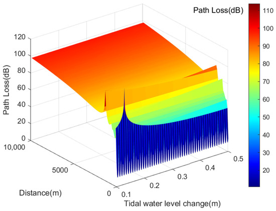
Figure 5.
Transmission Loss of AIS Base Station Signals under Different Tidal Water Level Variations.
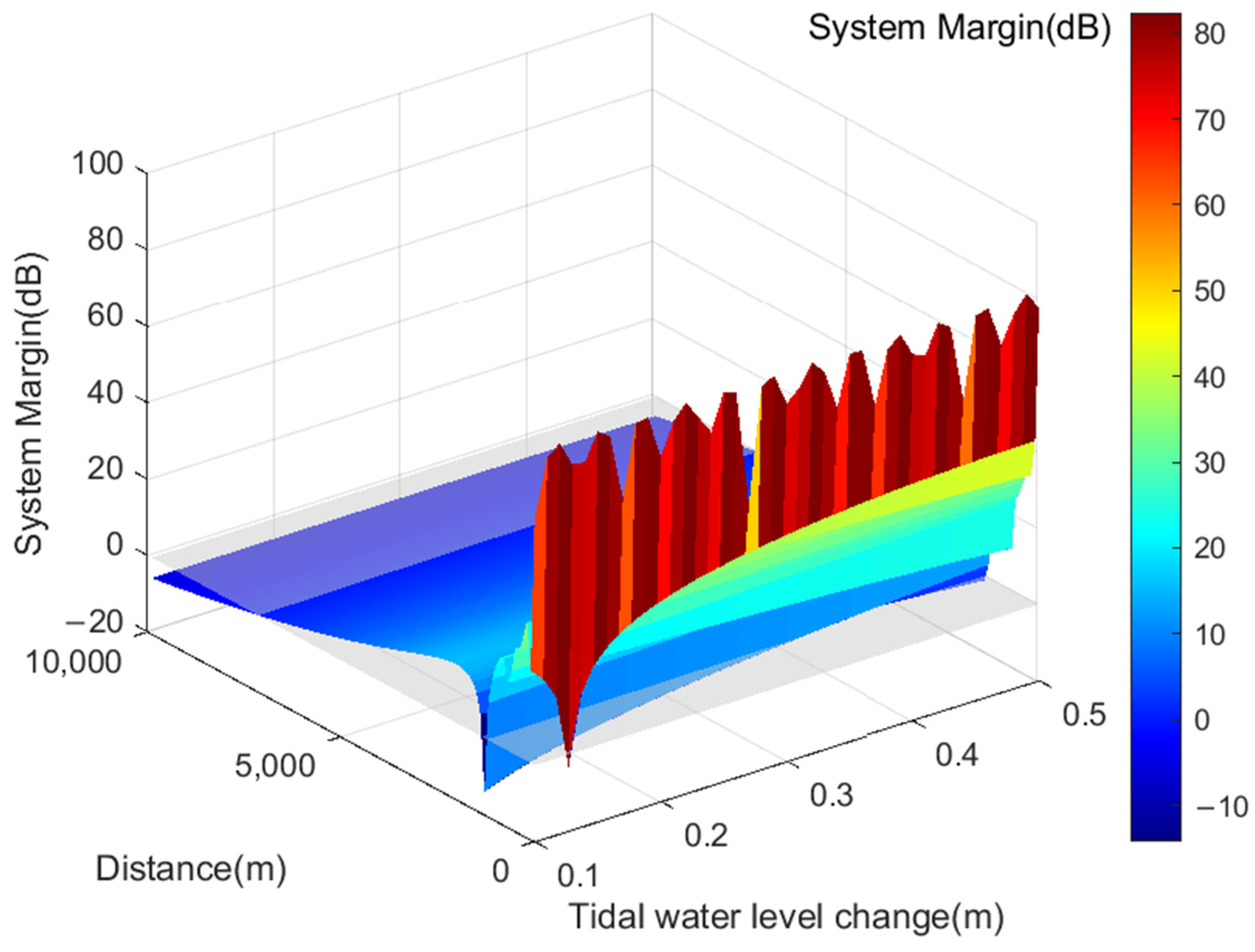
By integrating the transmission loss of VHF signals with the formula for VHF communication system margin, the coverage range of VHF signals under varying tidal water levels is derived, as illustrated in Figure 6. Upon analyzing the simulation results, it becomes evident that the coverage range of VHF signals spans from 55 km to 62 km when tidal water level variations range from 0.1 m to 0.5 m. Tidal water level fluctuations notably impact short-distance signal propagation. The interference between the direct path from the transmitting antenna to the receiving antenna and the reflected path on the horizontal plane introduces a phase difference between the two signals, resulting in significant signal attenuation and a decrease in coverage range.

Figure 6.
Service Radius of AIS Base Station Signals under Different Tidal Water Level Variations.
2.3. The Impact of Evaporation Duct on the Service Radius of AIS Base Station Signals
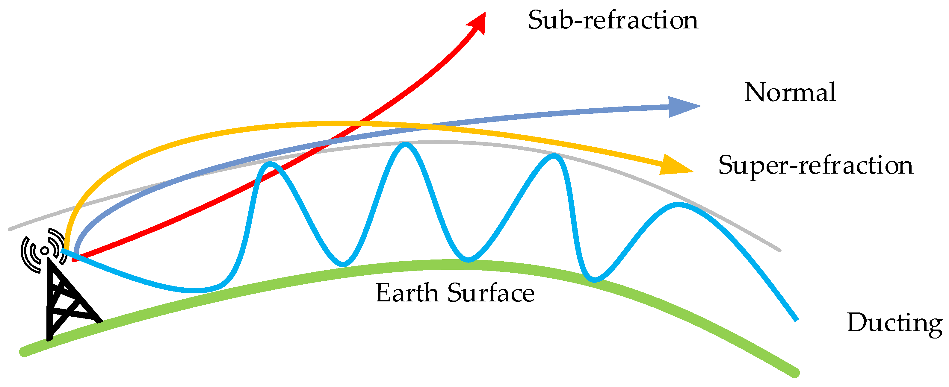
An evaporation duct is an atmospheric phenomenon usually found on the surface of oceans or lakes, which is formed by water vapor evaporation and temperature gradient changes. The occurrence probability of evaporation ducts and their height vary significantly based on geographical region, season, and time of day. Typically, evaporation ducts are more prevalent in low-latitude maritime regions during summer days, leading to higher EDH (Evaporation Duct Height). In the China Bohai Sea area, evaporation ducts are observed from March to August, peaking in May with EDH exceeding 30 m in certain localized spots. Conversely, the lowest evaporation duct heights are recorded in January, February, and December. The results presented in [22,23] show that the evaporation duct can affect the AIS base station signal’s propagation on the sea surface since the presence of the evaporation duct causes electromagnetic waves to be trapped in the evaporation duct layer, reducing the propagation loss of the trapped signal and leading to the phenomenon of over-the-horizon propagation. The VHF signals propagating on the sea surface are mainly based on the two-ray model, but the presence of the evaporation duct causes the receiver to receive refracted signals because of the refracted signal of the evaporation duct, as illustrated in Figure 7. Therefore, the influence of the evaporation duct on signal propagation loss should be considered when calculating the signal service radius of an AIS base station.
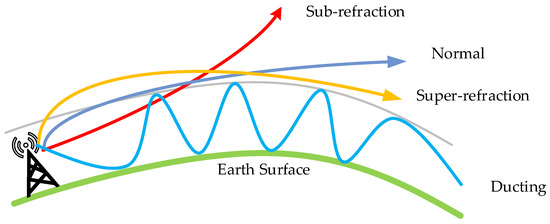
Figure 7.
Schematic of the AIS base station signal propagation in the presence of an evaporation duct.
As illustrated in Figure 7, when an evaporation duct is present, the AIS base station signal propagates through the sea surface using the three-ray propagation model. This model includes the direct signal emitted by the AIS base station, the signal reflected by the seawater, and the signal refracted due to the presence of the evaporation duct [24]. The model is defined as follows:
where is the wavelength of the AIS base station signal in meters and is the propagation distance of the AIS base station signal in meters, where can be calculated by Equation (19):
where and are the transmitting and receiving antenna heights in meters, respectively, and is the effective height of the evaporation duct. The annual average height of the evaporation duct is 13.0 m, and the maximum generally does not exceed 40.0 m [25].
At sea level, the air is saturated with water vapor, resulting in 100% relative humidity over the sea surface. As altitude increases, both temperature and water vapor content decrease. At a specific altitude, water vapor pressure equalizes with environmental pressure, ceasing its decrease with further altitude gain. Under favorable meteorological conditions, this scenario can lead to the formation of an evaporation duct layer. The height of this duct layer hinges on meteorological factors, notably air and water temperatures and relative humidity. A greater temperature differential between sea and air augments the duct’s height, while higher relative humidity diminishes it. The Paulus-Jeskes model, widely utilized for predicting evaporation ducts, employs input parameters, including sea surface temperature, atmospheric temperature at a height of at least 6 m, relative humidity, and wind speed. The model assumes atmospheric pressure at the sea surface to be 1000 hPa [26]. According to the Paulus-Jeskes model, the height of the evaporation duct is computed in four sequential steps:
- Step 1: To calculate the Richardson number Rib, the formula is as follows:
- Step 2: To calculate the Monin-Obukhov length using the Richardson number, the formula is as follows:
The calculation formula for the refractive index of seawater, , is as follows:
where represents the water vapor pressure of seawater at the ocean surface, and its expression is as follows:
Step 4: To determine the stability between the atmosphere and the ocean and select the method to calculate the evaporation duct height, we consider the following conditions. When , indicating a stable state where the air temperature around the ocean surface exceeds the sea surface temperature. If , then ; otherwise, if , the calculation formula for the evaporation duct height is as follows:
where the function is defined as follows:
where represents the surface roughness parameter.
If the calculated evaporation duct height from Equation (28) is found to be less than 0 or is greater than 1, then the evaporation duct height is recalculated as follows:
In the case of unstable atmospheric conditions (i.e., ), the evaporation duct height is given by
where the function is defined as follows:
where is a function that considers , so the expression for is as follows:
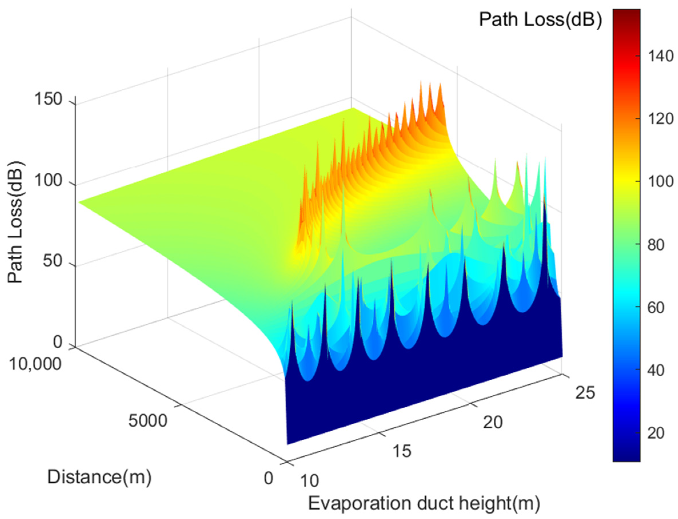
In summary, Figure 8 illustrates the calculated transmission loss of VHF signals at various effective heights of the evaporation duct. For propagation distances under 5 km, VHF signal transmission loss exhibits an oscillating pattern ranging from 10.6115 dB to 198.6850 dB. These points, where path loss significantly increases, are known as interference nulls. As the evaporation duct height increases, the last interference null shifts gradually to the right. When propagation distances exceed 5 km, the transmission loss of VHF signals shows a monotonically increasing trend due to the capturing effect of the evaporation duct on VHF frequency signals, resulting in gradual transmission loss growth.
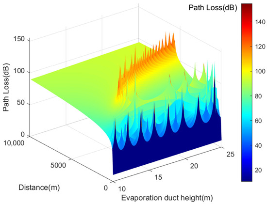
Figure 8.
Illustrates the transmission loss of AIS base station signals under different effective duct heights.
Figure 8 also demonstrates that for propagation distances of AIS base station signals under 5 km, their transmission loss exhibits a similar oscillating pattern, ranging from 10.6115 dB to 198.6850 dB. As the effective duct height increases, the position of the last interference null shifts to the right. When propagation distances exceed 5 km, AIS signal transmission loss shows a consistent increase, similarly influenced by the evaporation duct’s capturing effect on VHF frequency signals [27].
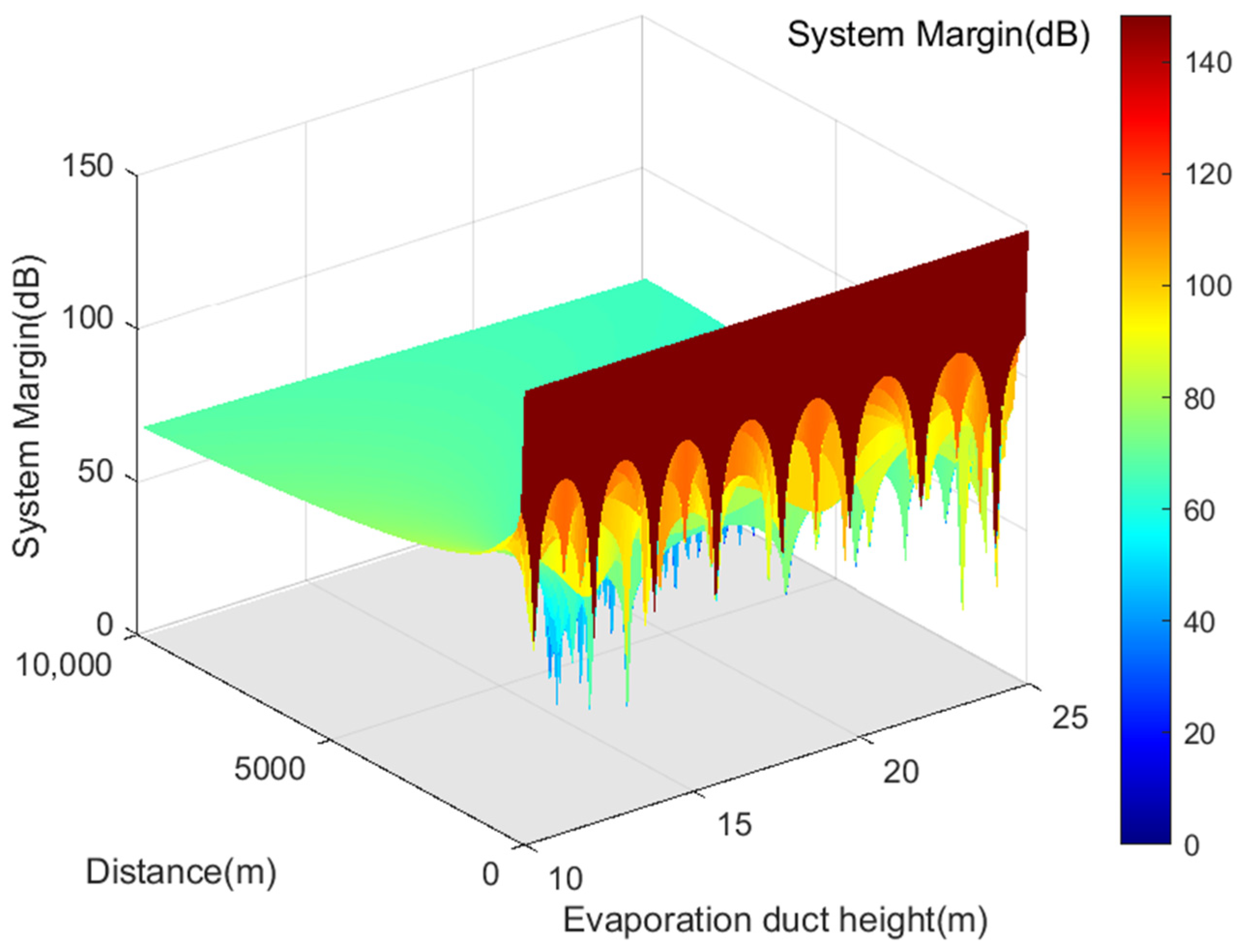
Moreover, Figure 9 presents the coverage range of VHF signals under different effective duct heights derived from the analysis of VHF signal transmission loss. It is observed that when the effective duct height ranges between 12 m and 18 m, the transmission loss of VHF signals is lower than free-space transmission loss due to the capturing effect of the evaporation duct. The AIS base station signal system maintains a positive margin, ensuring stable signal quality, and extends the coverage range of VHF signals beyond 100 km, facilitating beyond-line-of-sight propagation.
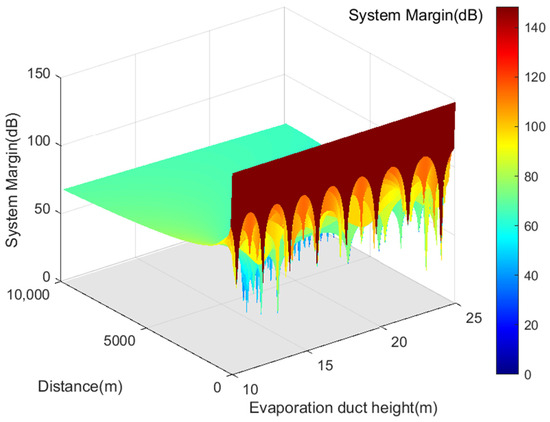
Figure 9.
Depicts the service radius of AIS base station signals under different effective duct heights.
3. Pattern of AIS Base Station Signal Service Radius Detection in Complex Sea Surface Environments
According to the discussion in Section 2 and considering the spare calculation formula of the VHF communication system, it is evident that the service radius of AIS base stations is primarily impacted by the transmission loss of AIS base station signals. Furthermore, due to the distinct maritime electromagnetic propagation environment, the transmission of AIS base station signals is notably susceptible to factors such as sea conditions and atmospheric conditions. Hence, building on the analysis of various maritime environmental factors affecting the service radius of AIS base station signals in Section 2 and integrating actual measurement data, a model for transmission loss of AIS base station signals under complex maritime conditions has been developed. This model has enabled further computation of the service radius of AIS base station signals under these conditions. A subsequent consistency analysis between the calculated service radius of AIS base stations and the ship-to-shore distance derived from telegram information is performed to evaluate the credibility of AIS base stations, establishing a pattern for monitoring AIS base station credibility based on service radius detection.
3.1. Calculation of AIS Base Station Signal Service Radius in Complex Sea Surface Environments
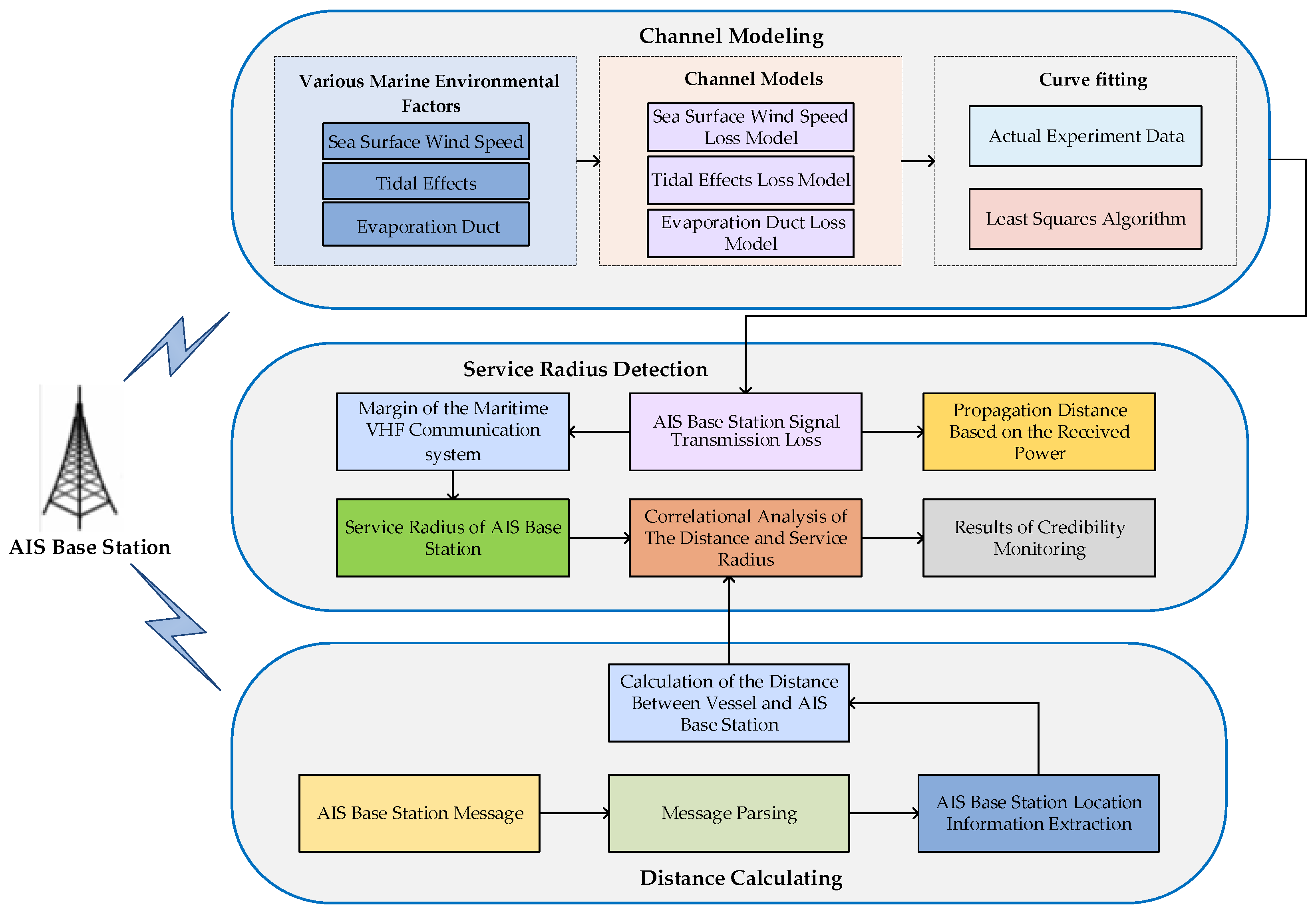
The primary framework of the AIS base station credibility monitoring method, which focuses on service radius detection patterns, is illustrated in Figure 10. Initially, the propagation environment of AIS base station signals is modeled, and the hydro-meteorological factors influencing the transmission loss are analyzed. A least squares algorithm is employed to fit the collected data, resulting in a transmission loss model for AIS base station signals under complex maritime conditions and an analysis of the model’s fit. By incorporating the spare capacity calculation of maritime communication systems, the service radius of AIS base stations in complex maritime conditions is computed. Concurrently, the coordinates of AIS base stations are obtained from parsing telegram information, allowing the calculation of the ship-to-shore distance. A matching analysis between this distance and the service radius of AIS base station signals is then conducted to assess the credibility of AIS base stations, providing a theoretical basis for credibility monitoring in complex maritime environments.
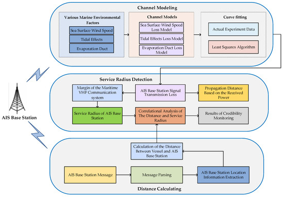
Figure 10.
Main architecture diagram of the AIS base station credibility monitoring pattern based on the service radius detection mode of AIS base stations.
By investigating sea surface factors such as wind speed, tidal variations, and evaporation duct height, this study explores their impact on AIS base station signal transmission loss. The relationship between the AIS base station service radius and these sea surface environmental factors can be expressed as follows:
where represents the transmission loss of AIS base station signals in a complex sea surface environment, denotes the environmental factor vector, represents various parameters describing the environmental factors, and represents the transmission loss influenced by sea surface wind speed, with u being the wind speed in meters per second (m/s). represents the transmission loss affected by tidal water level variations, and represents the height of tidal water level changes in meters (m). represents the transmission loss influenced by evaporation duct height. represents the air temperature in degrees Celsius, represents the sea surface temperature in degrees Celsius, represents the sea surface wind speed in m/s, represents the relative humidity, and represents the transmission distance in kilometers (km).
This paper initially outlines the trend of sea surface environmental changes influencing the AIS base station service radius using wireless channel modeling and simulation methods. Subsequently, a correction model for AIS base station signal transmission loss is proposed based on fitting experimental data with simulation results. By integrating this model with system margins, the AIS base station service radius is determined under various sea surface conditions. The AIS signal received power data utilized in this study were derived from maritime experiments conducted by the author’s research team in the waters of Dalian on 9 November 2016, as referenced [28].
In the experiment, the transmitter was mounted on the rooftop of Dalian Ocean University. The VHF signal transmission frequency used was 170 MHz, with a transmitter power of 37 dBm and an antenna height of approximately 26 m. The receiving antenna was positioned at around 3 m height. A signal generator served as the signal source, connected to a computer via LAN port using an Ethernet cable. Upon synchronization with a module comprising a rubidium clock and GNSS module, the signal generator and signal analyzer produced signals of specific power and frequency. These signals were then amplified by a power amplifier and transmitted through the transmitting antenna. The GNSS module calibrated the rubidium clock for precise time synchronization, minimizing data delay errors. The receiver and its antenna were installed on an experimental test boat, and the boat’s movement on the sea surface varied the distance between the transmitter and receiver. Figure 11 illustrates the boat’s navigation route, spanning from coordinates (38.8734° N, 121.5626° E) to (38.8044° N, 121.6034° E). During navigation, the onboard receiver was linked to the signal analyzer to analyze signal power, and the received data were saved to a designated path on the computer. The experimental data collected from this setup are presented in Table 1.
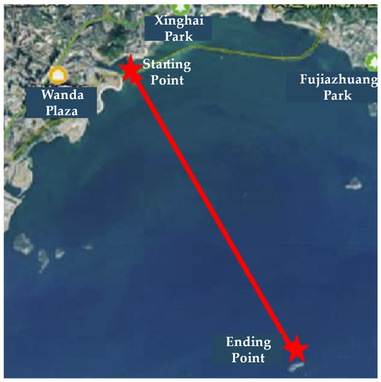
Figure 11.
Map of the Ship’s Movement Route with Two Red Stars as the Starting and Ending Points.

Table 1.
Experimental Measurements of Signal Received Power.
Table 1 displays the experimental data depicting received signal power at different transmission distances. Coupled with the signal transmission power, these data determine the transmission loss of the AIS signal. To establish a mathematical relationship between propagation distance and transmission loss in actual sea propagation conditions, appropriate fitting methods are applied to fit the experimental data. In this study, the least squares method is utilized for this purpose. As analyzed in Section 2, the AIS base station signal transmission loss is a function of the sea surface wind speed transmission loss , evaporation duct transmission loss , and tidal water level variation transmission loss . Therefore, the fitting function is defined as
where , and are undetermined constant coefficients. represents the transmission loss influenced by sea surface wind speed, with u being the wind speed in meters per second (m/s). represents the transmission loss affected by tidal water level variations, and represents the height of tidal water level changes in meters (m). represents the transmission loss influenced by evaporation duct height. represents the air temperature in degrees Celsius, represents the sea surface temperature in degrees Celsius, represents the sea surface wind speed in m/s, represents the relative humidity, and represents the propagation distance in kilometers (km).
In this study, the least squares method is utilized to fit and establish the model. Let represent the number of measured data sets, and the actual transmission loss is denoted as . The calculated transmission loss obtained from the fitting function Equation (35) is denoted as . According to the theory of least squares numerical fitting, there exists a certain difference between the predicted values of the fitting function and the transmission loss in the measured data. By considering the sum of squared errors to approach zero, the values of , and under this condition can be obtained:
By setting Equation (36) to its minimum value and applying calculus theory, we take the partial derivatives of both sides of the equation with respect to , and . Considering the infinitesimal derivatives as zero, we have:
That is,
By solving the above system of linear equations, the values of the unknown parameters , , and are obtained. Specifically, = 0.4873, = 0.3671, = 0.1417. With these values, the transmission loss of AIS base station signals in complex sea surface environments can be determined, which is
where represents the transmission loss influenced by sea surface wind speed, with u being the wind speed in meters per second (m/s). represents the transmission loss affected by tidal water level variations, and represents the height of tidal water level changes in meters (m). represents the transmission loss influenced by evaporation duct height. represents the air temperature in degrees Celsius, represents the sea surface temperature in degrees Celsius, represents the sea surface wind speed in m/s, represents the relative humidity, and represents the propagation distance in kilometers (km).
To validate the fitting degree, the adequacy of the obtained fitting function to actual data is assessed by evaluating the goodness of fit using the coefficient of determination . ranges between 0 and 1, with values closer to 1 indicating a stronger alignment of the fitting function with the actual data, and values nearer to 0 indicating a weaker alignment. A goodness of fit above 0.9 is generally deemed acceptable, while a value exceeding 0.95 signifies a highly effective fit [29]. The formula for calculating is as follows:
where represents the actual data, and represents the data on the fitted curve. Using the measured data in Table 1 to calculate the fitting degree of the curve fitted by Equation (39), the calculated result is 0.97338. This proves that Equation (39), representing the transmission loss of AIS base station signals in complex maritime environments, conforms well to the standards of fitting with the measured data.
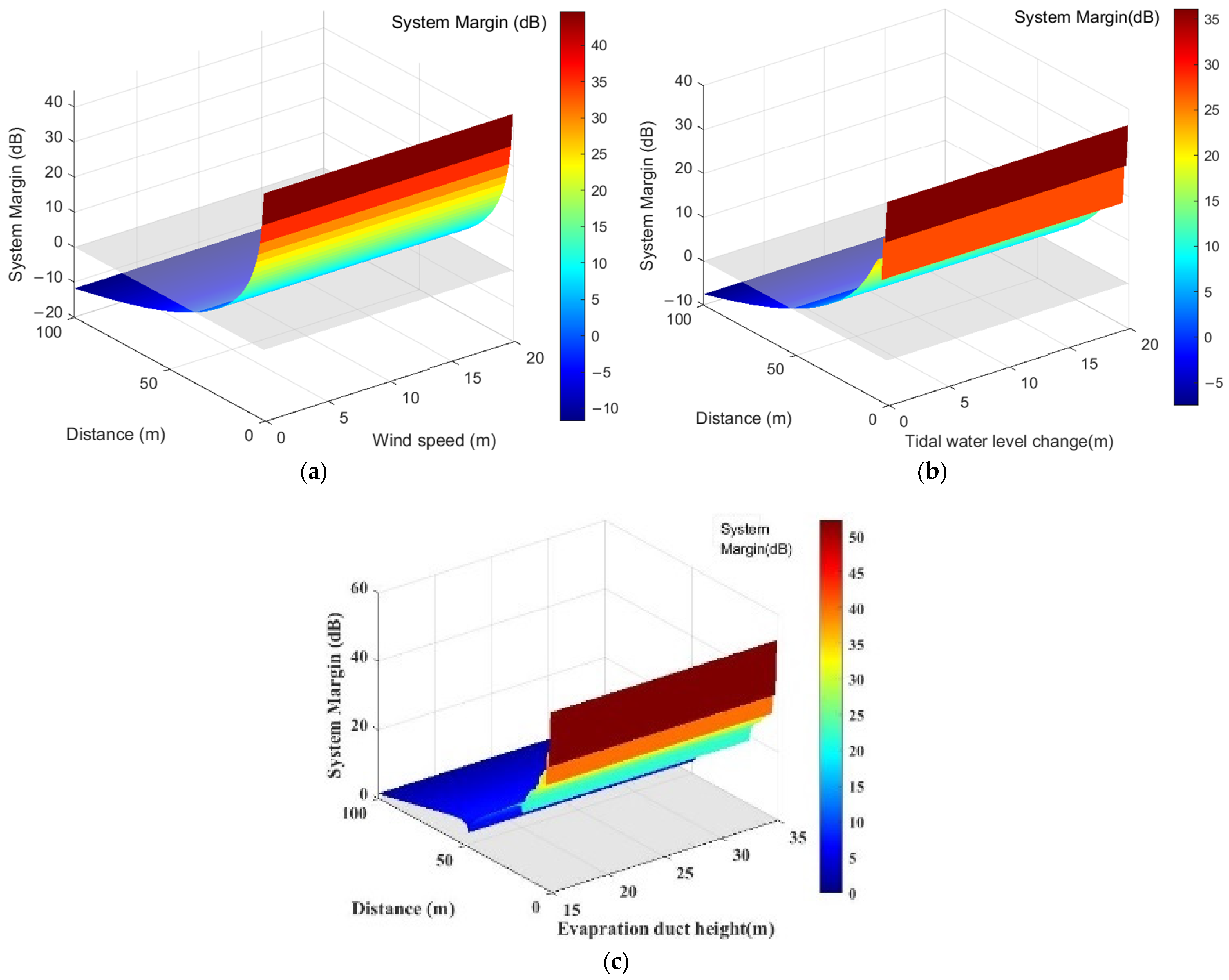
Therefore, under the same sea surface conditions, using Equations (15), (17) and (18), the transmission loss of AIS base station signals , , and at different distances is calculated. These values were then applied in the transmission loss Equation (39) of AIS base station signals in complex maritime environments to derive AIS base station transmission loss across different distances. Subsequently, based on Equation (5), the AIS base station service radius under different sea surface conditions is calculated, as shown in Figure 12.
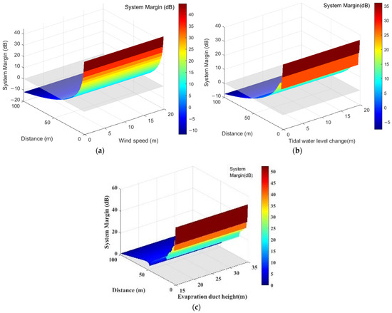
Figure 12.
Service Radius of AIS Base Station Signals under Different Sea Surface Conditions. (a) Wind speed changes; (b)Tidal water level changes; (c) evaporation duct height.
Figure 12 showcases the AIS base station signal service radius under varying sea surface conditions, encompassing changes in sea surface wind speed, tidal water levels, and effective evaporative waveguide height. The figure’s horizontal axis denotes shifts in sea surface environmental factors, while the vertical axis represents the system margin value. As distance increases, the system margin value decreases. When the system margin value remains above 0, the corresponding maximum transmission distance defines the AIS base station service radius. For instance, in Figure 12a, under conditions of 1 m tidal water level variation and 0 m evaporative waveguide height, increasing sea surface wind speed results in an AIS base station signal service radius of 19.4384 nautical miles. Similarly, Figure 12b shows a service radius of 22.13822 nautical miles with 2 m/s wind speed and 0 m evaporative waveguide height, varying with tidal water level changes. Figure 12c demonstrates that under evaporative waveguide conditions, the AIS base station signal service radius does not drop below 26.9978 nautical miles, ensuring continuous coverage.
3.2. Pattern Validation and Calculation of AIS Base Station Signal Service Radius
To validate the formula derived for estimating transmission losses in complex maritime settings and to precisely determine the AIS signal service radius, we compared the signal transmission distance calculated using current sea surface environmental factors in Formula (39) with the distance computed through the classic VHF signal transmission model, supported by actual test data. The established models employed in this comparison include the free space model, Okumura-Hata model, Egli model, and ITU-R P.1546 model. The correlation between transmission losses and signal transmission distances for each of these models is outlined below. (For this comparative study, the AIS signal frequency selected is 162.025 MHz).
- I.
- Free space model
Free space is defined as an infinitely vast, uniform, and lossless medium—essentially an ideal space. The propagation of radio waves in free space represents an ideal scenario. Assuming there are no obstacles along the propagation paths and both the transmitting and receiving antennas are isotropic, the transmission loss in free space is:
where denotes the wavelength of electromagnetic waves, represents the signal transmission distance (km), and is the operating frequency (MHz). From Formula (41), it is evident that the transmission loss in free space depends solely on the signal frequency and transmission distance. If the transmission distance increases by a factor of 10, the transmission loss along the transmitter and receiver paths increases by 20 dB.
- II.
- Okumura-Hata model
The Okumura-Hata model is an empirical model developed through statistical analysis of test data tailored for VHF and UHF frequency bands. This model employs the median path loss of field strength in quasi-flat urban terrain as a baseline and adjusts for various propagation environments and terrain conditions using correction factors.
The empirical formula for transmission loss in the Okumura-Hata model is
where denotes the operating frequency (MHz); is the signal transmission distance (km); represents the effective height of the transmitting antenna (m); is the effective height of the receiving antenna (m); is the receiving antenna height correction factor, which varies based on environmental factors, as calculated in Equations (43) and (44).
For the scenario of receiving antennas in small to medium-sized cities:
For the scenario of receiving antennas in large cities,
- III.
- Egli model
The Egli model is suitable for calculating wireless signal transmission losses in the frequency range of 90 to 1000 MHz. This model expands on the dual-path model used on flat ground by including losses over irregular terrains based on measurements. Using flat earth transmission losses as a basis, the Egli model provides a signal transmission loss calculation formula for when < 10 m:
where represents the operating frequency (MHz); is the signal transmission distance (km); and denote the effective heights of the transmitting and receiving antennas (m); is the terrain correction factor (dB), which fluctuates based on the frequency. For the AIS signal frequency of 162.025 MHz, the formula for is as detailed in Equation (46):
where represents the terrain undulation height; if is less than 15 m, can be disregarded.
- IV.
- ITU-1546 model
The International Telecommunication Union (ITU) has introduced a radio signal propagation model for the frequency range of 30 MHz to 3000 MHz, known as the ITU-R P.1546 model. This model offers a detailed calculation of signal transmission losses, incorporating both measured data and theoretical analysis, resulting in
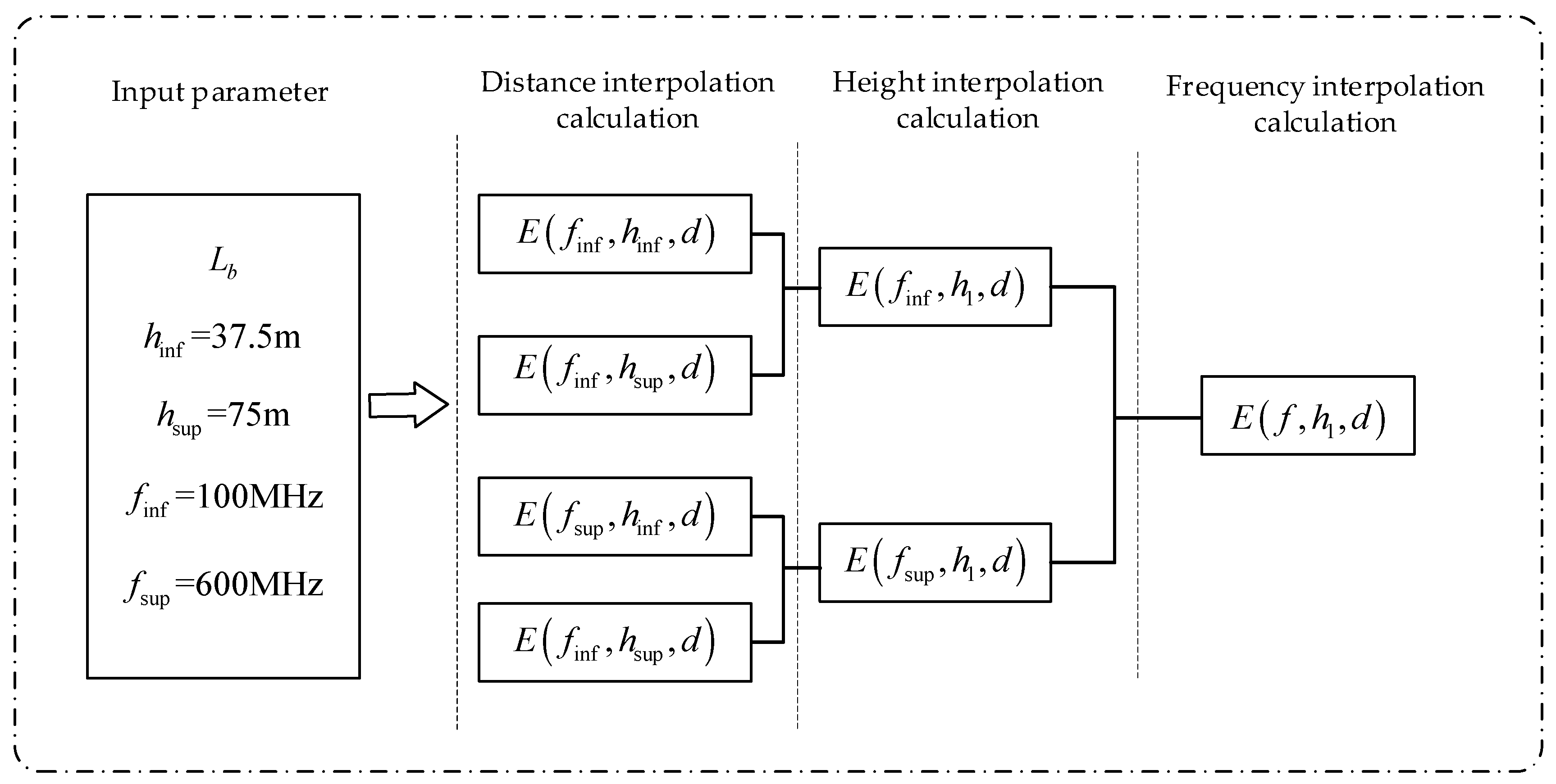
where denotes the operating frequency (MHz), and represents the field strength value (). According to the ITU-R P.1546 recommendation, the calculation of the signal field strength value relies on propagation parameters. The nominal values for transmission distance, signal frequency, and base station antenna height are established sequentially. Following the completion of the field strength interpolation based on distance, frequency, and base station antenna height, the calculation is executed using Formula (48):
where is the signal transmission distance (km), is the closest nominal distance less than , is the closest nominal distance greater than , is the field strength corresponding to transmission distance , and is the field strength corresponding to transmission distance . Therefore, the calculation process of the signal strength values for AIS signals using the ITU-R P.1546 model is summarized in Figure 13.
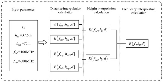
Figure 13.
AIS Signal Field Strength Calculation Method based on the ITU-R P.1546 Model.
As depicted in Figure 13, represents the signal transmission loss, is the height of the transmitting antenna, is the nearest nominal height less than , is the nearest nominal height greater than , is the nearest nominal frequency less than , is the nearest nominal frequency greater than , and is the signal transmission distance. To compute the signal field strength, the process begins with interpolation on the signal transmission distance, proceeds with interpolation on the field strengths at two designated heights, and concludes with extrapolation on the field strengths at two nominal frequencies. This methodology derives the AIS signal field strength value. Utilizing the ITU-R P.1546 model parameters, the values employed for the comparative experiments in this study are presented in Table 2.
Table 2.
Base station propagation parameters.
- V.
- Comparative Experiment
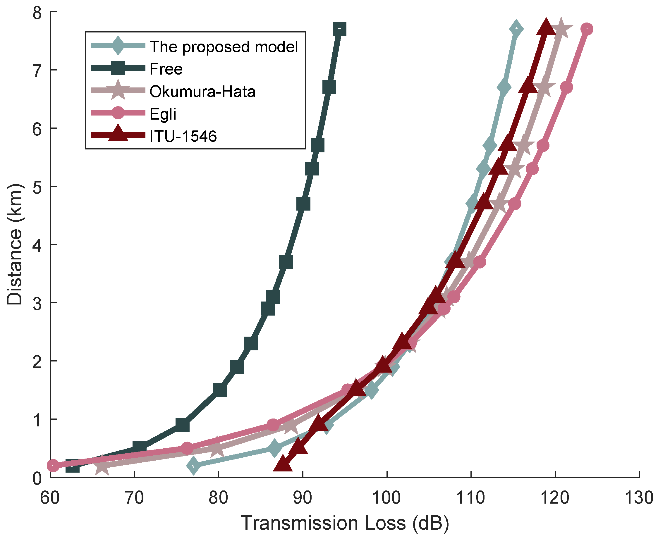
Regarding the meteorological conditions in the maritime test area on the date of the actual sea trial executed by the author’s research team, the recorded data were as follows: sea surface wind speed at 3.0595 m/s, relative humidity at 52.9557%, air temperature at 4.5 °C, water temperature at 6.9 °C, and tide level at 94.3 cm. These metrics were gathered from the marine meteorological readings monitored at the Dalian Laohutan station on 9 November 2016, supplied by the China Oceanic Administration and the National Meteorological Science Data Center. The collected meteorological parameters were inputted into various transmission models to estimate the signal transmission losses, as illustrated in Figure 14.

Figure 14.
Transmission Loss of AIS Base Station Signals Under Different Models.
The findings illustrated in Figure 14 highlight significant variances in AIS signal transmission distance calculations across different propagation loss models, even when utilizing identical sea surface meteorological conditions. To further scrutinize the accuracy of each model in calculating signal transmission distances, this paper examines 13 sets of measured data and juxtaposes these with the calculated distances by each model, as detailed in Table 1. Moreover, Equation (40) is employed to compute the goodness of fit between each model and the measured data, with the results tabulated in Table 3.
Table 3.
Comparison table of transmission distance data between measured data and calculated data from various models.
Analysis from Table 3 reveals that the goodness of fit for the signal transmission distance calculated by the AIS base station signal transmission loss model proposed in this paper in complex sea surface environments is 0.97338. This value surpasses those achieved by various classical signal transmission loss models, highlighting that the model proposed here offers a more precise calculation of signal transmission distances compared to other classical models. The free space transmission loss model recorded the lowest goodness of fit at 0.22639, with the Egli model following suit. This disparity arises because these models primarily focus on signal frequency and terrain fluctuations as the key parameters in calculating transmission losses while overlooking additional factors that influence signal transmission losses. Both the Okumura-Hata model and the ITU-R P.1546 model, which consider signal frequency and terrain fluctuations, also incorporate the geographical location of the antenna and adjust signal transmission losses accordingly. However, these models do not account for the fact that AIS base station signals predominantly operate in maritime environments where complex and fluctuating sea conditions cause signal attenuation and losses during propagation. Thus, the accuracy of the Okumura-Hata model and the ITU-R P.1546 model in calculating transmission distances of AIS base station signals over sea surfaces is inadequate. The AIS base station signal transmission loss model introduced in this paper is specifically tailored to address the effects of complex sea surface factors on AIS base station signal transmission losses. It quantitatively calculates the signal transmission losses of AIS base stations under various sea surface conditions and describes the mathematical principles governing AIS base station signal transmission distances in these environments. Therefore, the model presented in this paper achieves the best correlation between the calculated AIS signal transmission distances and the measured data.
4. AIS Base Station Credibility Monitoring Experiment
AIS base stations enable bidirectional communication with vessels using VHF signals, facilitating information exchange between ships and from ship to shore. The effectiveness of these functions relies crucially on the credibility of AIS base stations to ensure that the information broadcast to vessels within their coverage area is accurate and credible. AIS “spoofing” involves disseminating false telegram information beyond the AIS base station’s service radius through identity deception, which can create confusion and disrupt vessels within the service radius as well. Therefore, this section presents the design of a credibility monitoring method for AIS base stations operating in complex maritime environments. This method capitalizes on the unique MMSI of each base station, correlating it with location, and integrates this data with the service radius and distance of AIS base station signals to monitor credibility effectively.
4.1. Specific Method
In challenging maritime settings, the algorithm for Automatic Identification System (AIS) base station credibility monitoring, which utilizes the service radius detection pattern, adheres to the following steps:
Step 1: Extract the MMSI code, location data, and other relevant parameters from the AIS base station telegram received by the vessel.
Step 2: Confirm the validity of the base station’s MMSI code through a search on the China Maritime Safety Administration’s official website. If the MMSI code is determined to be invalid, the base station is deemed untrustworthy. Conversely, if the MMSI code is valid, proceed to further evaluations.
Step 3: Compare the location details of the base station, as indicated by the MMSI code and retrieved from the AIS shore-based interference monitoring and emergency response system’s distributed database, against the location information parsed from the telegram. A discrepancy between these datasets indicates untrustworthiness at this stage; if they align, move to the next checks.
The AIS Shore-Based Interference Monitoring and Emergency Response System is a comprehensive management system for shore station telegrams developed independently by the author’s research team in collaboration with relevant maritime authority information departments. This system’s distributed database archives all legitimate telegrams from AIS shore stations [30].
Step 4: Perform a matching test using the MMSI code and location from the received AIS base station telegram, then compare other telegram parameters against those of legitimate telegrams previously issued by the base station, stored in the distributed database. Any discrepancies at this point suggest untrustworthiness. If all parameters match, continue with the subsequent steps.
Step 5: Calculate the service radius () of the AIS base station based on the current marine meteorological conditions.
Step 6: Determine the distance () between the ship and the location specified in the telegram.
Step 7: Assess whether the ship-to-shore distance () exceeds the base station’s service radius (). If is greater than , the base station’s signal is theoretically unable to reach the ship, indicating a false signal. If is less than , the ship is within the base station’s service range, suggesting that signal reception is possible, though further verification is required.
Step 8: Compute the transmission distance of the AIS base station signal () at this time using the signal transmission loss model developed in this study for complex marine environments.
Step 9: Compare the transmission distance of the base station’s signal () with the calculated ship-to-shore distance (). If is not equal to (±97.3%), the received signal strength does not align with the expected value, leading to a classification of the base station as untrustworthy. Conversely, when is equal to (±97.3%), the AIS base station is considered trustworthy, as it falls within the model’s accuracy range for complex marine environments.
The flowchart of the AIS base station credibility monitoring method based on the service radius detection pattern is illustrated in Figure 15.
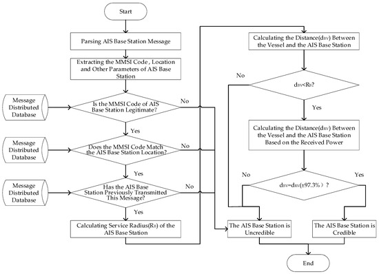
Figure 15.
The flowchart of the AIS base station credibility monitoring method based on the service radius detection pattern.
For calculating the distance between the vessel and the base station, this study employs the Haversine formula, which accurately computes the distance between two latitude and longitude points on Earth’s surface, typically measured in nautical miles, kilometers, or miles. Assuming the position coordinates of the vessel and the base station are denoted as and , respectively, the specific expression is as follows:
where is the haversine function, , = 6378 km is the radius of the Earth. If the base station location coordinates extracted from AIS messages are used along with the vessel’s position coordinates to calculate distance by substituting them into Equation (49), distance represents the transmission distance of AIS base station signals calculated using the transmission loss model proposed in this paper for complex maritime environments.
To practically apply the AIS Base Station credibility monitoring method, this paper has developed a three-tiered AIS Base Station credibility monitoring system within a Client/Server (C/S) model. This system encompasses AIS data preprocessing, AIS Base Station credibility monitoring, and system-human interaction functionalities. The system login interface is illustrated in Figure 16.

Figure 16.
Login Interface of AIS Base Station Credibility Monitoring System.
4.2. Experimental Results and Analysis
This section validates the effectiveness of the AIS base station credibility monitoring method using the service radius detection pattern through various scenarios, including illegal base station MMSIs, “spoofing” base stations existing within and outside the AIS base station service radius, and scenarios devoid of “spoofing” base stations.
- I.
- Existing illegal MMSI base station
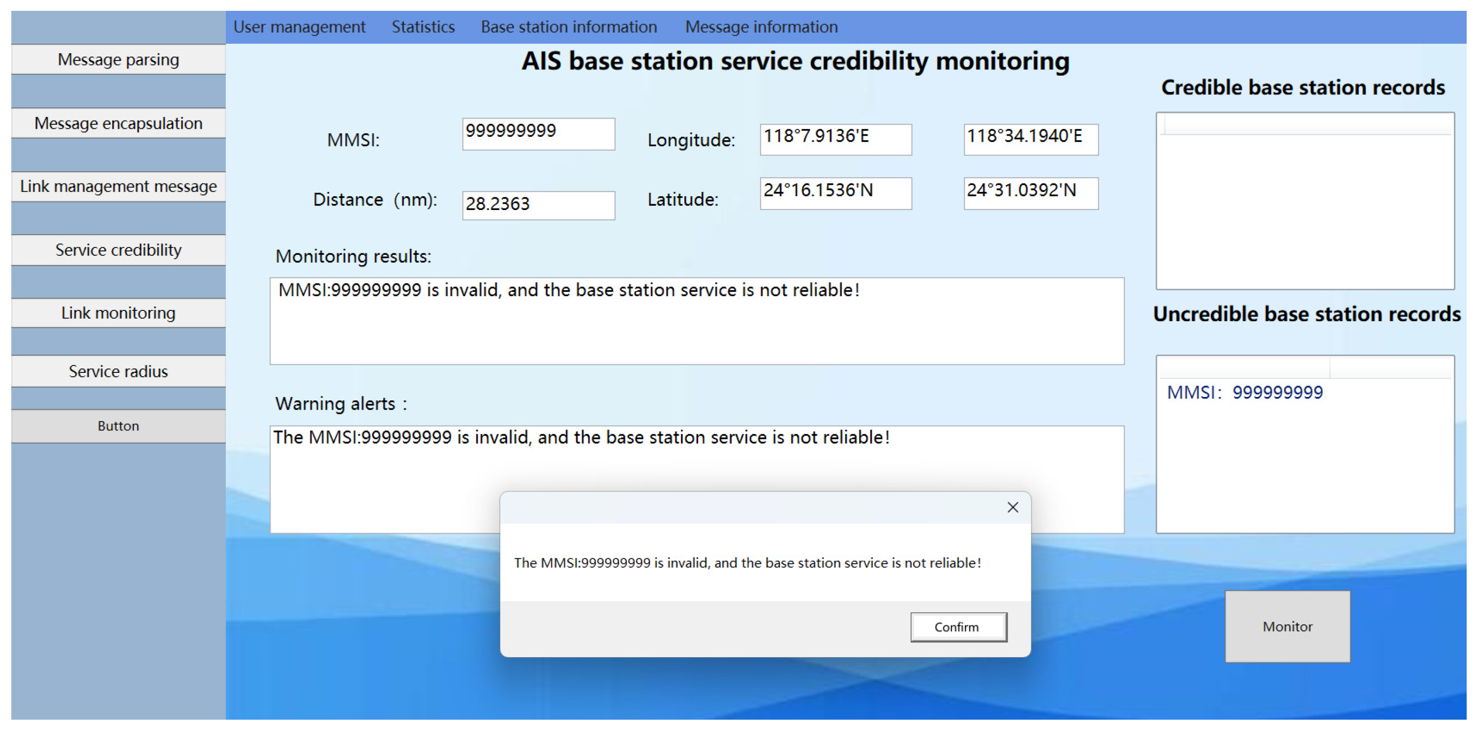
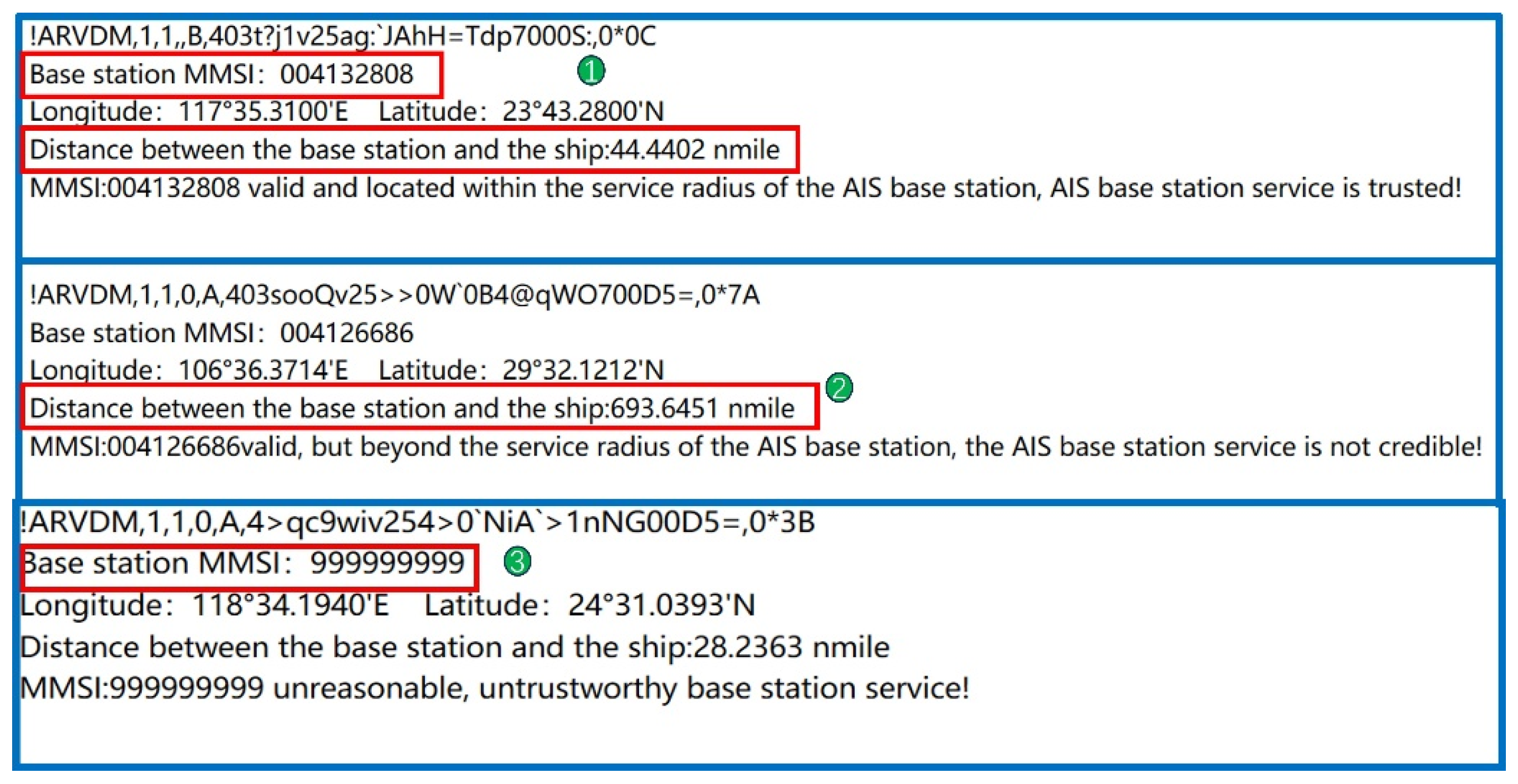
The AIS ship received the following position message from the AIS base station: !ARVDM,1,1,0,A,4>qc9wiv254>0‘NiA’>1nNG00D5=,0*3B. The MMSI of the AIS base station, listed as 999999999, with position coordinates at (24°31.0393′ N, 118°34.1940′ E), was checked. The distance calculated between the AIS base station and the ship was 28.2363 nautical miles. Upon verification, the MMSI code was found to be invalid, indicating that the base station is unauthorized, as shown Figure 17. Therefore, the ship cannot receive legitimate messages from the AIS base station. This suggests that the AIS base station data received by the ship originates from an unauthorized source, indicating the presence of an unauthorized base station between the ship and the base station, thus rendering the AIS base station untrustworthy. The experimental results are shown as number 3 in Figure 18.

Figure 17.
Results of the experimental system monitoring with illegal base station MMSIs set.
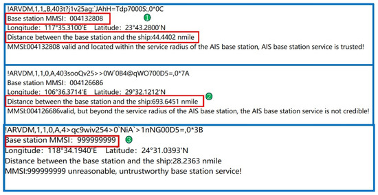
Figure 18.
AIS base station service credibility monitoring results for three distinct scenarios (* in this figure is the checksum field identifier).
The monitoring results of the AIS base station credibility monitoring system are depicted in Figure 17. The MMSI of the illegal base station is recorded as 999999999, with coordinates (24°30.7920′ N, 118°34.1940′ E). Upon entering this illegal MMSI into the AIS base station credibility monitoring interface, the system indicates that the base station’s MMSI is invalid, thereby confirming the system’s capability to detect illegal MMSI stations.
Referring to the monitoring outcomes shown in Figure 18, it is noted that item 1 reflects the AIS base station credibility monitoring result under conditions of no interference, indicating the AIS base station service is credible. Item 2 pertains to the AIS base station credibility monitoring result when beyond the AIS base station signal service radius, and item 3 relates to the AIS base station credibility monitoring result for an illegal base station MMSI. In scenarios 2 and 3, the AIS base station credibility monitoring results are deemed uncredible. In summary, the legality of the MMSI code in the message received by the ship from the AIS base station can be verified to ascertain whether the base station is illegal. An illegal MMSI code signifies that the current AIS base station is untrustworthy. Conversely, a legal MMSI code allows for the calculation of the distance between the base station and the ship. By comparing this distance with the AIS base station signal service radius, the monitoring of AIS base station credibility can be effectively conducted.
- II.
- “Spoofing” base stations existing outside the AIS base station service radius
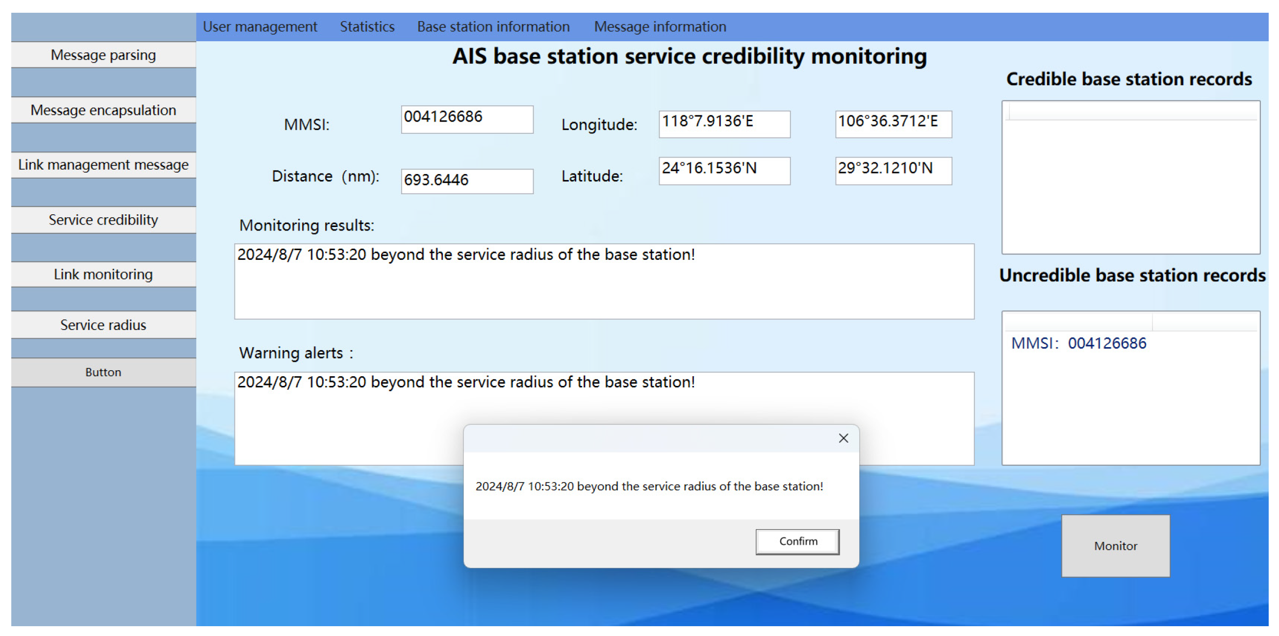
The AIS ship received the following position message from the AIS base station: !ARVDM,1,1,0,A,403sooQv25>>0W`0B4@qWO700D5=,0*7A. The MMSI of the AIS base station is recorded as 004126686, with position coordinates at (29°32.1212′ N, 106°36.3712′ E). The signal service radius for this AIS base station is 46.5085 nautical miles, while the calculated distance between the AIS base station and the ship is 693.6445 nautical miles. Upon verification, the MMSI code of the AIS base station was found to be valid. However, the distance between the AIS base station and the ship far exceeds the AIS base station’s signal service radius, implying that the ship cannot receive the messages sent by the AIS base station. This suggests that the AIS base station data received by the ship originates from an unauthorized source, indicating the presence of an unauthorized base station between the ship and the base station, thus rendering the AIS base station untrustworthy. The experimental results are shown as number 2 in Figure 18.
The monitoring results of the AIS base station credibility monitoring system, depicted in Figure 19, indicate that while the base station service radius remains constant, the distance between the ship and the base station has increased to 693.6440 nautical miles. This distance surpasses the AIS base station signal service radius. Consequently, the system concludes that the AIS base station is untrustworthy, affirming the effectiveness of the AIS base station credibility monitoring system in assessing the trustworthiness of AIS base stations.

Figure 19.
Results of the experimental system monitoring with “spoofing” base stations present outside the AIS base station service radius.
- III.
- “Spoofing” base stations existing within the AIS base station service radius
When a “spoofing” base station is within the service radius of an AIS base station, monitoring its credibility involves three scenarios: In the first scenario, after decoding the received AIS base station message to determine the position of the base station, if this position does not correspond with the position stored in the distributed message database for the base station’s MMSI, the AIS base station is considered untrustworthy. In the second scenario, if the base station’s position in the AIS message aligns with the stored position for the base station’s MMSI in the distributed message database, but other parameters in the message differ from those of previously authenticated messages associated with that base station, the AIS base station is regarded as untrustworthy. In the third scenario, if the base station’s position in the AIS message coincides with the stored position for the base station’s MMSI in the distributed message database, and the other parameters in the message are consistent with those of previously legitimate messages. However, if the distance between the ship and shore calculated from the base station’s position exceeds the signal propagation distance determined from the actual received power, the AIS base station is deemed untrustworthy. The following discussion describes the verification experiments for these scenarios.
In the first scenario, the AIS ship received a message from an AIS base station as follows: !ARVDM,1,1,0,A403t?i1v25agI`dKu<F?IAA00D5=,0*41. After decoding, the MMSI code for the AIS base station was identified as 004132804, with the base station’s coordinates pinpointed at (38°52.09′ N, 121°33.33′ E). Verification through the official China Maritime Safety Administration website confirmed the validity of this MMSI. However, the position data stored for this MMSI in the distributed message database was (24°16.1534′ N, 118°7.9137′ E), markedly different from the coordinates obtained from the base station’s message. Consequently, this discrepancy renders the AIS base station uncredible, as illustrated in Figure 20 of the monitoring results.
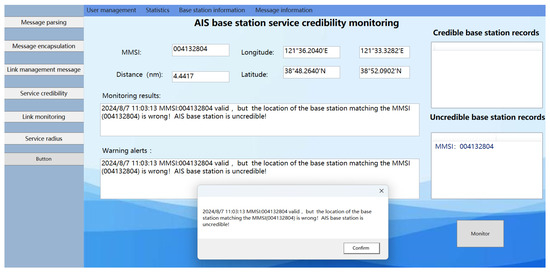
Figure 20.
Results of the experimental system monitoring with “spoofing” base stations present within the AIS base station service radius for the location mismatch with MMSI code scenario.
In the second scenario, the AIS ship received an AIS base station message as follows: !ARVDM,1,1,0,A403t?i1v269gD`dKu<F?IAC02D5=,0*17. Upon parsing, the details of the message are outlined in Table 4.
Table 4.
Parsing parameters of the base station for invalid parameters.
After checking the MMSI code listed in Table 4 on the official website of the China Maritime Safety Administration, it was confirmed that the MMSI code for this AIS base station is valid. Further investigation into the distributed message database showed that the position information for the base station indicated by this MMSI code is (38°52.09′ N, 121°33.33′ E), which matches the AIS base station position information obtained through message parsing. However, a comparison within the database revealed discrepancies in the message parameters: in previously sent legitimate messages from this base station, the electronic position fixing device type was 7, and the RAIM flag was 0. In contrast, in Table 4, the electronic position fixing device type in the AIS base station message is 3, and the RAIM flag is 1, which contradicts the parameters of the legitimate messages previously sent by this base station. Therefore, in this instance, the base station is deemed untrustworthy, as illustrated in the monitoring results shown in Figure 21.
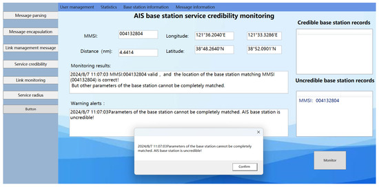
Figure 21.
Results of the experimental system monitoring with “spoofing” base stations present within the AIS base station service radius for the illegitimate message scenario.
In the third scenario, the AIS ship received a message from an AIS base station as follows: !ARVDM,1,1,0,A403t?j1v25agI`dE>HF=UkG00D5:,0*46. After decoding, the details of the message are presented in Table 5.
Table 5.
Parsing parameters of the base station for the legitimate message.
After verification through the official website of the China Maritime Safety Administration, the MMSI code for this AIS base station was confirmed to be legitimate. Additionally, the position information (38°54.72′ N, 121°36.474′ E) and other message parameters stored in the distributed message database for this MMSI code matched the received information. However, the experiment described in Section 3.1 reveals that when the ship is located at (38°48.26′ N, 121°36.20′ E), the received signal power is −68 dBm. According to the signal propagation loss model for AIS base station signal transmission in complex maritime environments detailed in this document, the calculated signal propagation distance is 6.15 km. In contrast, the distance between the ship and the shore calculated using Equation (37) from the base station position (38°54.72′ N, 121°36.474′ E) is 12 km, which exceeds the expected range with a goodness fitting of 97.3% for the propagation distance. This discrepancy suggests that the signal from the base station, as reported in the base station message, does not align with the actual received signal power. Therefore, in this case, the AIS base station is considered uncredible, as depicted in the monitoring results in Figure 22.
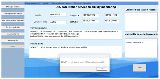
Figure 22.
Results of the experimental system monitoring with “Spoofing” base stations present within the AIS base station service radius for the ship-to-shore distance beyond the expected range scenario.
- IV.
- Scenarios devoid of “spoofing” base stations
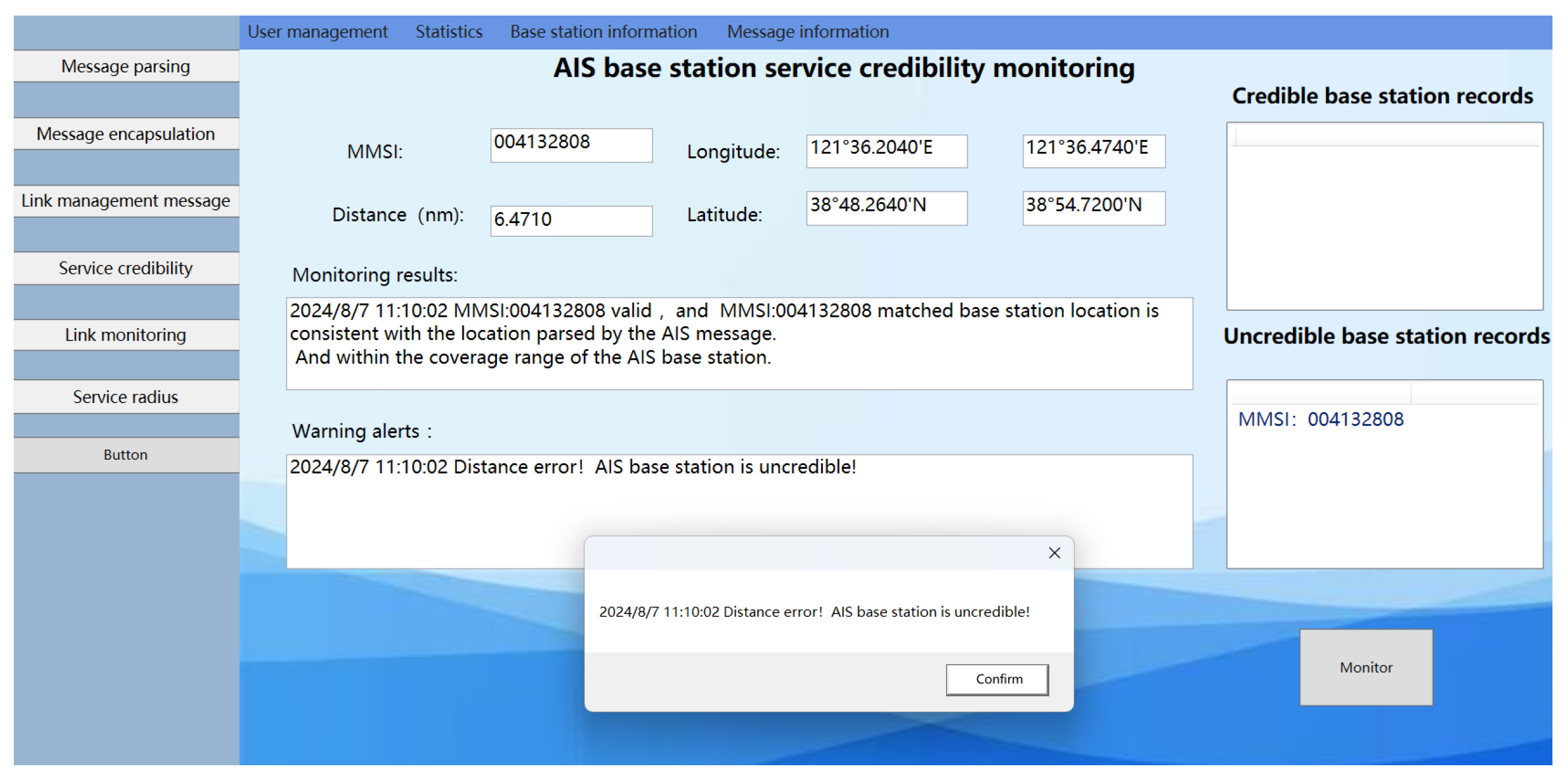
The AIS ship received a location information message from an AIS base station as follows: !ARVDM,1,1,B,403t?j 1v25ag:`JAhH=Tdp7000S:,0*0C. After decoding, the MMSI code for the AIS base station was identified as 004132808, with a MID of 413, indicating that the base station is geographically located in the Chinese region at coordinates (23°43.2800′ N, 117°35.3104′ E). Verification through the official website of the China Maritime Safety Administration confirmed that the MMSI code for this AIS base station is legitimate. Furthermore, the position information (23°43.2800′ N, 117°35.3104′ E) and other message parameters stored in the distributed message database for this MMSI code correspond with the received information. According to the experiment detailed in Section 3.1, when the ship is positioned at a specific location (23°42.114′ N, 117°31.89′ E), the received signal power is −68 dBm. Based on the AIS base station signal transmission loss model in complex maritime environments described in this document, the calculated signal propagation distance is 6.15 km. Given the base station’s coordinates (23°43.2800′N, 117°35.3104′ E), the calculated distance to the shore using Equation (37) is 6.2 km, fitting within the expected range with a goodness of fit of 97.3% for the propagation distance. This consistency indicates that the signal transmitted from the base station location, as reported in the base station message, matches the actual received signal power at the receiver. Therefore, in this case, the AIS base station is deemed trustworthy, as shown in the monitoring results in Figure 23.
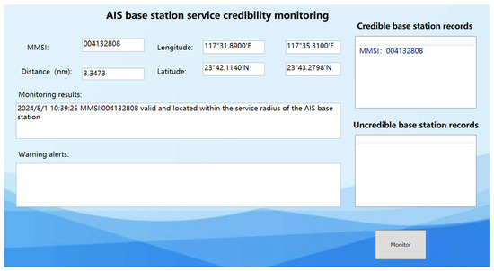
Figure 23.
Results of the experimental system monitoring with scenarios devoid of “spoofing” base stations.
5. Conclusions
This paper introduces a method for detecting AIS Base Station Credibility based on a service radius detection pattern, employing a signal transmission loss model for AIS base stations in complex sea conditions. Initially, the study examines factors such as the effective height of evaporative waveguide, sea surface wave height, and tidal variations, assessing their impact on signal transmission loss and service radius of AIS base stations in real oceanic propagation environments. Moreover, utilizing field-measured data, a signal transmission loss model for AIS base stations in complex maritime environments was established. The experimental findings reveal that the model achieves a goodness of fit of 0.97338, demonstrating superior accuracy compared to traditional models like free space, Okumura-Hata, Egli, and ITU-R P.1546. This model was then applied to precisely calculate the AIS base station signal service radius and transmission distance. Following this, by determining the distance between the AIS base station location in the message and the ship and comparing this distance with the AIS base station service radius and the ship-to-shore distance derived from the actual received power, a matching analysis was carried out. This analysis paved the way for the creation of an AIS base station trustworthiness monitoring method based on the AIS base station service radius detection pattern. The efficacy of this method was tested under various interference scenarios. The experimental outcomes confirm that the proposed AIS base station trustworthiness monitoring method based on the service radius detection pattern can effectively identify scenarios where the base station presents an illegal MMSI code, a mismatch between the MMSI code and the base station position, inconsistencies between the base station message and legitimate message parameters, a ship-to-shore distance that exceeds the AIS base station signal service radius, and discrepancies between ship-to-shore distance and signal transmission distance, thus identifying “spoofing” AIS base stations. This method plays a crucial role in enhancing maritime traffic safety, optimizing shipping efficiency, and mitigating maritime accidents.
Author Contributions
X.W. and Q.H. supervised the work, arranged the architecture, and contributed to the writing of the paper; Y.W. and X.W. designed the measurement scheme, carried out the simulations, and wrote the paper; L.F. analyzed and compiled the data. All authors have read and agreed to the published version of the manuscript.
Funding
This research was partially supported by the National Natural Science Foundation of China (No. 62301106) and the National Key Research and Development Program of China (No. 2021YFB3901502).
Institutional Review Board Statement
Not applicable.
Informed Consent Statement
Not applicable.
Data Availability Statement
All data have been provided in this paper. Further inquiries can be directed to the corresponding authors.
Conflicts of Interest
The authors declare no conflict of interest.
References
- Forsberg, J. Cybersecurity of Maritime Communication Systems: Spoofing Attacks against Ais and Dsc. 2022. Available online: https://www.diva-portal.org/smash/get/diva2:1705102/FULLTEXT01.pdf (accessed on 1 November 2023).
- Li, W.; Liu, C.; Li, J.; Ji, X. Study on the Impact of Virtual AtoN Setting on AIS in Harbour Areas. In Proceedings of the International Conference in Communications, Signal Processing, and Systems, Changbaishan, China, 24–25 July 2021; Volume 878, pp. 407–415. [Google Scholar]
- Xu, G.; Wan, T.; Wang, D.; Guo, J.; Cao, Y. Research on the AIS Decoding System Based on Raspberry Pi in the Dynamic Monitoring of the Yangtze River Waterway. In Proceedings of the 2021 6th International Conference on Intelligent Transportation Engineering (ICITE 2021), Beijing, China, 17–19 September 2021; pp. 870–879. [Google Scholar]
- Chen, M.-Y.; Wu, H.-T. An Automatic-Identification-System-Based Vessel Security System. IEEE Trans. Ind. Inform. 2023, 19, 870–879. [Google Scholar] [CrossRef]
- Jaskólski, K.; Marchel, Ł.; Felski, A.; Jaskólski, M.; Specht, M. Automatic identification system (AIS) dynamic data integrity monitoring and trajectory tracking based on the simultaneous localization and mapping (SLAM) process model. Sensors 2021, 21, 8430. [Google Scholar] [CrossRef] [PubMed]
- Maulidi, A.; Abdullah, M.; Handani, D. Virtual private network (VPN) model for AIS real time monitoring. IOP Conf. Ser. Earth Environ. Sci. 2022, 1081, 012028. [Google Scholar] [CrossRef]
- Wolsing, K.; Roepert, L.; Bauer, J.; Wehrle, K. Anomaly detection in maritime AIS tracks: A review of recent approaches. J. Mar. Sci. Eng. 2022, 10, 112. [Google Scholar] [CrossRef]
- Lv, T.; Tang, P.; Zhang, J. A Real-Time AIS Data Cleaning and Indicator Analysis Algorithm Based on Stream Computing. Sci. Program. 2023, 2023, 8345603. [Google Scholar] [CrossRef]
- Shyshkin, O. Cybersecurity Providing for Maritime Automatic Identification System. In Proceedings of the IEEE 41st International Conference on Electronics and Nanotechnology (ELNANO), Kyiv, Ukraine, 10–14 October 2022; pp. 736–740. [Google Scholar]
- Louart, M.; Szkolnik, J.J.; Boudraa, A.O.; Le Lann, J.-C.; Le Roy, F. Detection of AIS messages falsifications and spoofing by checking messages compliance with TDMA protocol. Digit. Signal Process. 2023, 136, 103983. [Google Scholar] [CrossRef]
- d’Afflisio, E.; Braca, P.; Willett, P. Malicious AIS Spoofing and Abnormal Stealth Deviations: A Comprehensive Statistical Framework for Maritime Anomaly Detection. IEEE Trans. Aerosp. Electron. Syst. 2021, 57, 2093–2108. [Google Scholar] [CrossRef]
- Rong, H.; Teixeira, A.P.; Guedes Soares, C. Data mining approach to shipping route characterization and anomaly detection based on AIS data. Ocean Eng. 2020, 198, 106936. [Google Scholar] [CrossRef]
- Guo, S.; Mou, J.; Chen, L.; Chen, P. An anomaly detection method for AIS trajectory based on kinematic interpolation. J. Mar. Sci. Eng. 2021, 9, 609. [Google Scholar] [CrossRef]
- Chen, J. Prediction Method of Offshore VHF Wireless Coverage Based on ITU-RP.1546-3 Proposal. Navig. Technol. 2009, 39–43. Available online: https://www.itu.int/dms_pubrec/itu-r/rec/p/R-REC-P.1546-5-201309-I!!PDF-C.pdf (accessed on 5 September 2023).
- GB/T 39620—2020[S]; Technical Requirements for Coastal Automatic Identification System (AIS) Base Station. China Standards Publishing House: Beijing, China, 2020; pp. 6–7. Available online: http://c.gb688.cn/bzgk/gb/showGb?type=online&hcno=B28EFD7F44950419AAE92D1D36B9679C (accessed on 1 November 2023).
- Hu, Y.; Xu, L.; Gao, J.; Jia, P.; Li, B.; Xu, Y. Analysis of Marine Wireless Communication Channel under High Sea Conditions. In Proceedings of the 2022 IEEE 5th International Conference on Electronic Information and Communication Technology (ICEICT), Hefei, China, 21–23 August 2022; pp. 274–277. [Google Scholar]
- Jiménez, P.A.; Dudhia, J. On the need to modify the sea surface roughness formulation over shallow waters. J. Appl. Meteorol. Climatol. 2018, 57, 1101–1110. [Google Scholar] [CrossRef]
- Li, F.; Shui, Y.; Liang, J.; Yang, K.; Yu, J. Ship-to-ship maritime wireless channel modeling under various sea state conditions based on REL model. Front. Mar. Sci. 2023, 10, 1134286. [Google Scholar] [CrossRef]
- Huai, S.; Zhang, S.; Wang, X.; Zhang, J. A Novel Adaptive Noise Resistance Method Used for AIS Real-Time Signal Detection. Chin. J. Electron. 2020, 29, 327–336. [Google Scholar] [CrossRef]
- Mitayani, A.; Nurkahfi, G.N.; Mardi Marta Dinata, M. Path Loss Model of the Maritime Wireless Communication in the Seas of Indonesia. In Proceedings of the 2020 International Conference on Radar, Antenna, Microwave, Electronics, and Telecommunications (ICRAMET), Tangerang, Indonesia, 18–20 November 2020; pp. 97–101. [Google Scholar]
- Gaitan, M.G.; d’Orey, P.M.; Santos, P.M.; Ribeiro, M.; Pinto, L.; Almeida, L.; De Sousa, J.B. Wireless Radio Link Design to Improve Near-Shore Communication with Surface Nodes on Tidal Waters. In Proceedings of the OCEANS 2021: San Diego–Porto, San Diego, CA, USA, 20–23 September 2021; pp. 1–8. [Google Scholar]
- Robinson, L.; Newe, T.; Burke, J.; Toal, D. An Experimental Study of the Effects of the Evaporation Duct on Microwave Propagation. In Proceedings of the OCEANS 2019 MTS/IEEE SEATTLE, Seattle, WA, USA, 17–19 June 2019; pp. 1–5. [Google Scholar]
- Yang, F.; Yang, K.-D.; Shi, Y.; Wang, S.-W.; Zhang, H.; Zhao, Y.-M.; Hu, D.-W.; Dong, G.-Y. Impact of Evaporation Duct on Line-of-Sight Propagation of Electromagnetic Waves. J. Phys. Conf. Ser. 2023, 2486, 012060. [Google Scholar] [CrossRef]
- Habib, A.; Moh, S. Wireless Channel Models for Over-the-Sea Communication: A Comparative Study. Appl. Sci. 2019, 9, 443. [Google Scholar] [CrossRef]
- Zhao, W.; Zhao, J.; Li, J.; Zhao, D.; Huang, L.; Zhu, J.; Lu, J.; Wang, X. An Evaporation Duct Height Prediction Model Based on a Long Short-Term Memory Neural Network. IEEE Trans. Antennas Propagat. 2021, 69, 7795–7804. [Google Scholar] [CrossRef]
- Cruz, V.S.; Assis, F.; Schnitman, L. Simulation of the Effects of Evaporation Ducts on Maritime Wireless Communication. Wirel. Netw. 2021, 27, 4677–4691. [Google Scholar] [CrossRef]
- Reul, N.; Grodsky, S.A.; Yueh, S. Sea Surface Salinity Estimates from Spaceborne L-Band Radiometers: An Overview of the First Decade of Observation (2010–2019). Remote Sens. Environ. 2020, 242, 111769. [Google Scholar] [CrossRef]
- Yang, Q. The Character Analysis of Costal VHF Signal Propagation. Master’s Thesis, Dalian Maritime University, Dalian, China, 2017. [Google Scholar]
- Sun, J. Assessing Goodness of Fit in Confirmatory Factor Analysis. Meas. Eval. Couns. Dev. 2005, 37, 240–256. [Google Scholar] [CrossRef]
- Li, J. Monitoring and Emergency Operating System On AIS Base Station Management Messages. Master’s Thesis, Dalian Maritime University, Dalian, China, June 2018. [Google Scholar]


Disclaimer/Publisher’s Note: The statements, opinions and data contained in all publications are solely those of the individual author(s) and contributor(s) and not of MDPI and/or the editor(s). MDPI and/or the editor(s) disclaim responsibility for any injury to people or property resulting from any ideas, methods, instructions or products referred to in the content. |
© 2024 by the authors. Licensee MDPI, Basel, Switzerland. This article is an open access article distributed under the terms and conditions of the Creative Commons Attribution (CC BY) license (https://creativecommons.org/licenses/by/4.0/).