Vessel Trajectory Prediction for Enhanced Maritime Navigation Safety: A Novel Hybrid Methodology

Abstract

The accurate prediction of vessel trajectory is of crucial importance in order to improve navigational efficiency, optimize routes, enhance the effectiveness of search and rescue operations at sea, and ensure maritime safety. However, the spatial interaction among vessels can have a certain impact on the prediction accuracy of the models. To overcome such a problem in predicting the vessel trajectory, this research proposes a novel hybrid methodology incorporating the graph attention network (GAT) and long short-term memory network (LSTM). The proposed GAT-LSTM model can comprehensively consider spatio-temporal features in the prediction process, which is expected to significantly improve the accuracy and robustness of the trajectory prediction. The Automatic Identification System (AIS) data from the surrounding waters of Xiamen Port is collected and utilized as the empirical case for model validation. The experimental results demonstrate that the GAT-LSTM model outperforms the best baseline model in terms of the reduction on the average displacement error and final displacement error, which are 44.52% and 56.20%, respectively. These improvements will translate into more accurate vessel trajectories, helping to minimize route deviations and improve the accuracy of collision avoidance systems, so that this research can effectively provide support for warning about potential collisions and reducing the risk of maritime accidents.

1. Introduction

Maritime transportation serves as a vital pillar for the global economy and international trade, and has emerged as a key component in maintaining global supply chains and fostering global economic exchanges [1,2]. Over the past decade, there has been a significant increase in the density of maritime traffic flow and vessel movement. While this growth has provided substantial impetus for global economic development, it has also introduced a range of challenges and risks to navigation safety and resource management [3,4]. The incidence of ship collisions, groundings, and other safety accidents has escalated, posing serious threats to human lives, environmental conservation, and economic interests [5]. In this context, the effective management and analysis of massive navigation data have become the key tasks in preventing and addressing safety hazards. To achieve this objective, data derived from Automatic Identification Systems (AISs) have become one of the most prevalent data sources and widely applied for assessing navigation risks due to their rich spatio-temporal information on vessels [6,7]. Further, the accurate prediction of vessel trajectories based on the collected AIS data is essential in order to provide critical navigational advice and collision avoidance warning information to crew members, which plays an important role in mitigating the risk of maritime traffic accidents and enhance overall navigation safety. However, the real-time vessel trajectory prediction from extensive AIS data remains a formidable task that is heavily reliant on the selected methodologies [8].

Academically, trajectory prediction has garnered widespread research attention across various domains such as vehicles, pedestrians, and ships. In the early stages of vessel trajectory prediction research, researchers primarily used physical models and linear motion models to achieve a preliminary ship trajectory prediction. Subsequently, techniques like Kalman filters [9], Gaussian mixture models [10], and support vector machines [11] were introduced to improve the prediction accuracy. With technological progress and the need to handle more complex scenarios, subsequent studies have incorporated more sophisticated methods, such as deep-learning and sequence prediction models, which can capture the intricate dependencies and nonlinear features of time-series data more effectively. However, most current deep-learning methods only consider the temporal characteristics of ship trajectory data, resulting in limitations to a single prediction task and challenges in achieving the necessary accuracy for practical applications [12]. Furthermore, the future movement trajectory of vessels is influenced by a multitude of factors mainly from two perspectives: the environmental factors (i.e., weather, ocean currents, and traffic conditions) and the vessel-related factors (i.e., the previous navigation route of the ship, and the movement patterns of surrounding ships) that exhibit pronounced nonlinear and dynamic characteristics. A reliable prediction of the vessel trajectory should consider both types of factors.

To overcome the aforementioned limitations, this paper introduces an innovative hybrid approach for vessel trajectory prediction that combines the graph attention network (GAT) and long short-term memory network (LSTM). Utilizing preprocessed historical AIS data from targeted water areas, vessel trajectory samples are obtained for the development of the GAT-LSTM hybrid prediction model. The GAT component is designed to extract spatial features from the vessel network graphs, while the LSTM component captures the temporal correlations within the trajectory data. Consequently, this hybrid model takes into account both temporal and spatial features in the prediction process.

The primary innovations and contributions of this paper are as follows:

(1)

A novel hybrid vessel trajectory prediction method integrating GAT and LSTM is proposed to balance the extraction of spatial and temporal features effectively. More importantly, it provides a more comprehensive consideration of the vessel movement spatial relationship compared to traditional methods.

(2)

Given the particular attention to nodes that significantly impact the navigational behavior of the target vessel, a refined approach for modelling vessel interactions by dynamically assigning different learning weights to neighboring nodes based on their distances from the target vessel is introduced in this research. The application of such an approach could not only reflect real-world scenarios more accurately, but also enhance the prediction performance of the proposed model.

(3)

Through the empirical analysis using real AIS data, the proposed method is proven to surpass other baseline methods in terms of prediction accuracy and robustness, demonstrating the reliability and the superiority of this hybrid methodology.

The structure of the paper is as follows: Section 2 provides an overview of related works on vessel trajectory prediction. Section 3 details the research questions addressed in this work and outlines the proposed methodology for developing the GAT-LSTM model. Section 4 presents the empirical data utilized in this study, along with the experimental design and result analysis. Finally, Section 5 offers a summary of the paper and discusses the potential future research direction.

2. Review of Related Works

In this section, a brief overview of the research on vessel trajectory prediction is provided. Specifically, according to the prediction methods applied, the relevant research is categorized into three groups: physical-model-based, statistical- and machine-learning-based and deep-learning-based trajectory prediction methods.

2.1. Vessel Trajectory Prediction Based on Physical Models

Physical-model-based trajectory prediction methods typically rely on physical laws and kinematic models, and the prediction of a vessel’s next position does not involve learning the vessel’s movement patterns from historical trajectories. Instead, it is directly inferred from the established vessel motion model based on the current position and navigation speed of the vessel. The common methods based on physical models mainly include filtering algorithms and Markov chain algorithms.

The filtering algorithm is a recursive algorithm with low computational complexity, suitable for real-time application scenarios such as ship trajectory prediction. Tong et al. [9] proposed a trajectory prediction strategy based on a Kalman filter (KF), which achieves the accurate prediction of vessel trajectories by filtering the node position information in the vessel trajectory sequence. Jaskólski [13] utilized AIS data and discrete KF techniques to estimate missing vessel trajectory sequences. Fossen et al. [14] employed an extended KF to process real-time AIS data and used it as the basis for ship trajectory prediction. Mazzarella et al. [15] proposed a Bayesian ship trajectory prediction model based on a particle filter, which demonstrated good performance in strait and inland river scenarios. Perera et al. [16] introduced a method for predicting ship navigation states using an extended KF, which can predict the position and heading of vessels in the short term. However, the hybrid dual Kalman filter model developed by Zhou et al. [17] is only suitable for short-term traffic flow prediction and poses certain challenges for long-term prediction. Zhang et al. [18] combined the original hidden Markov models (HMMs) with wavelet analysis for predicting the trajectory of large ships, where the wavelet analysis aimed to reduce error accumulation and improve prediction accuracy. However, this model can only predict the next position of the ship and cannot simulate the continuous motion behavior of the ship. Cheng et al. [19] adopted an improved Markov model that comprehensively considers the temporal and spatial continuity of trajectories for local trajectory prediction, improving the prediction accuracy of traditional Markov models.

2.2. Vessel Trajectory Prediction Based on Statistics and Machine Learning

The trajectory prediction method based on statistics and machine-learning algorithms mainly learns the ship motion mode from the historical data to predict the ship’s future trajectory. Such methods include the Bayesian model, Gaussian mixture model (GMM), support vector machine (SVM) and random forest (RF).

Murray and Perera [20] proposed a trajectory prediction algorithm based on single-point neighborhood search, which searches the historical trajectory data through the current position of the target object and matches the next position with the highest probability from the historical trajectory distribution to achieve prediction. Although this algorithm can provide relatively accurate trajectory predictions within about 15 min, its effective operation requires a large amount of historical data. Due to the fact that a single probability model might not be able to describe the ship motion influenced by multiple factors, subsequent researchers have developed trajectory prediction models using multiple probability distributions. The GMM is one of the widely applied approaches. Dalsnes et al. [21] proposed a data-driven short-term ship trajectory prediction method based on the GMM and provided an estimate of the uncertainty for the prediction results. Rong et al. [22] modelled the ship motion patterns as Gaussian processes, thereby adeptly addressing the uncertainty challenges inherent in trajectory prediction. Murray and Perera [23] applied principal component analysis to generate features for each trajectory, then used an unsupervised GMM to cluster these trajectories, and predicted the trajectories of each cluster to generate multiple potential ship trajectories. The experimental results indicate that at least one of these trajectories matches the actual ship trajectory. Liu et al. [24] proposed a trajectory prediction model based on the SVM, selecting ship speed, heading, timestamp, longitude, and latitude as sample features, and using an adaptive chaotic differential evolution algorithm to optimize the model parameters, thereby improving the prediction accuracy and convergence speed to a certain extent. However, the SVM has relatively weak generalization ability and is prone to falling into local optima. The RF method is an ensemble-learning algorithm consisting of many decision trees. RF generates numerous decision trees using random variables and data, and then aggregates the predictions of these trees. Zhang et al. [25] proposed a data-driven ship destination prediction model based on RF. They measured the similarity between a ship’s travel trajectory and historical trajectories, predicting the destination of the ship to be the destination of the historical trajectory with the highest similarity. Although this study did not directly predict ship trajectories, the prediction of ship destinations indirectly reflects the predictive capability of this method.

However, the traditional trajectory prediction methods mentioned above highly rely on mathematical formulae and assumptions, and their performance is limited by a large number of prior assumptions. The GMM depends on a finite mixture of Gaussian distributions to model the trajectory data. In dynamic maritime environments, where ship movements can be influenced by many unpredictable factors, the GMM may struggle to capture the full complexity of the motion patterns. The assumption of Gaussian distributions may not adequately represent the diversity and evolution of ship trajectories, leading to reduced accuracy in such scenarios. On the other hand, RF aggregates predictions from multiple decision trees to handle large datasets, but it struggles with capturing dynamic interactions and temporal de-pendencies, potentially performing poorly in complex and rapidly changing maritime environments. Therefore, they are usually only applicable to specific scenarios and may not provide reliable predictions in complex maritime traffic situations with dy-namic environments.

2.3. Vessel Trajectory Prediction Based on Deep Learning

The primary concept of deep-learning-based trajectory prediction methods is to extract vessel movement characteristics from extensive historical AIS data and train a neural network model to predict vessel movement trends. Nguyen et al. [26] divided the sea area into a spatial grid, employing the latest ship trajectories as inputs to a sequence-to-sequence model for motion prediction. Capobianco et al. [27] proposed a vessel trajectory prediction model using an encoder–decoder recurrent neural network (RNN) framework, which captures the spatio-temporal dependencies in sequence data. Due to its unique model structure, the RNN can effectively address the limitations of traditional feedforward neural networks in handling variable length sequences and capturing long-distance dependencies in sequences. Zhang et al. [28] established an LSTM network model for ship trajectory prediction after preprocessing AIS data for integrity and accuracy. LSTM solves the gradient vanishing and explosion problems in the RNN with its unique gating mechanism. In addition, Forti et al. [29] developed a neural Seq2seq model with an LSTM encoder–decoder architecture to enhance the overall prediction performance by capturing long-term temporal dependencies in AIS data. Suo et al. [30] used a GRU-based model and the density-based spatial clustering of applications with noise (DBSCAN) algorithm to extract and optimize main trajectories. Experimental results show that this model exhibits a similar prediction accuracy to LSTM while improving the computational time efficiency.

In order to further improve the accuracy of trajectory prediction, Liu et al. [31] improved the bidirectional long short-term memory (Bi-LSTM) model, and proposed an efficient routing algorithm based on the predicted trajectory and the confidence of each prediction step to achieve efficient communication performance. Additionally, integrating attention mechanisms into deep-learning models helps focus on key parts of the input data, thereby more effectively capturing significant relationships and features within the data. This has proven beneficial in enhancing model performance, particularly in areas such as image processing and time-series data prediction [32,33,34]. Zhao et al. [35] created an encoder–decoder learning model with LSTM units and attention mechanisms, using the LSTM units to extract relationships between historical trajectories and current states, and employing global attention and multi-head self-attention to enhance prediction accuracy and efficiency.

Although the aforementioned models effectively model the temporal information in ship trajectories, they often fail to fully address social interaction factors among ships, leading to suboptimal predictions in complex maritime environments with intersecting ship routes. In response to this issue, Zhang et al. [36] combined convolutional neural networks (CNNs) with RNNs to capture both the temporal and spatial attributes of vessel trajectories. While RNNs handle time-series data effectively, they struggle with long-term dependencies. With the development of graph neural networks, some researchers have made certain research progress by incorporating these into prediction models [37]. Graph convolutional networks (GCNs) model social relationships by representing ships as nodes and their interactions as edges, offering a new approach for trajectory prediction. Feng et al. [38] proposed a method that integrates spatio-temporal graph convolutional neural networks (STGCNNs) and a temporal extrapolation convolutional neural network to predict future ship trajectories. Liu et al. [39] developed a spatio-temporal multigraph transformation network model based on the GCN and transformers for synchronous multi-ship trajectory prediction. However, it struggles with the inductive task of handling dynamic graphs. Additionally, Liu et al. [40] proposed a spatio-temporal multigraph convolution network (STMGCN) framework within a mobile-edge-computing paradigm, utilizing multiple graph types and optimization techniques for more reliable predictions. However, GCN-based approaches heavily rely on predefined graph structures to capture the static attributes of ships, thereby overlooking their dynamic interactions. Zhao et al. [41] introduced a model combining graph attention networks (GAT) and LSTM to predict ship trajectories, validated on three real datasets. However, this study constructs the graph network by dividing a single ship’s trajectory into multiple sub-trajectory segments and focuses on the spatio-temporal characteristics of individual segments, limiting its ability to capture dynamic interactions between ships.

To address this limitation, this paper develops network graphs that reflect the positional relationships among ships, with weights assigned based on distance to encapsulate the spatial–temporal characteristics of vessel movements. By integrating the GAT and LSTM, this approach captures the multifaceted and intricate spatial and temporal interaction features inherent in ship trajectories, leading to more dependable trajectory predictions. This methodology offers valuable insights for maritime traffic management and collision avoidance while also contributing to the enhancement of safety and efficiency in maritime navigation.

3. Methodology

3.1. Problem Description

In this paper, the research on vessel trajectory prediction is primarily grounded in extensive historical AIS data, which encompass a wealth of spatio-temporal details pertaining to vessel movements. To enhance clarity and facilitate comprehension, this section delineates the fundamental concepts and terminology associated with vessel trajectory prediction as referenced throughout the paper.

Vessel trajectory $\mathit{T}$. The trajectory of a vessel is a series of spatio-temporal coordinates arranged in chronological order based on the position data of the vessel. The trajectory of any selected vessel k in a water area can be defined as $T_k=\{P_1,P_2,\dots P_n\}$, where n is the number of vessel trajectory points, and $P_i(1\le i\le n)$ is the coordinates of the vessel at the i-th trajectory point.

Vessel network graph $\mathit{G}$. A vessel network graph is an abstract data structure used to represent the spatial relationships and interactions between vessels. In this graph, the vessels are modelled as nodes, and their relationships are modelled as edges. Figure 1 illustrates the process of creating a vessel network and shows the vessel network graphs stacked along the time dimension.

In each layer, the vessel network graph describes the position and spatial relationship of the vessel at the current time step. The vessel network graph at time step t is defined as $G^t=(V^t,E^t)$, where V is a set of nodes representing vessels, and E is a set of edges representing the interactions between these vessels. Specifically, $V^t=\left\{{v^t}_n\right|n=\mathrm{1,2},\dots ,N\}$, and $E^t=\left\{{e^t}_{i,j}\right|i,j=\mathrm{1,2},\dots ,N\}$, where N represents the number of vessels, ${v^t}_n$ denotes the motion features of the n-th vessel at time t, and ${e^t}_{i,j}$ represents the interaction between the i-th and j-th vessels at time t.

Adjacency matrix A. The adjacency matrix is used to describe the connection relationships between nodes in a vessel network graph. It is a two-dimensional array with a size of N × N, where N represents the number of nodes (vessels) in the graph. The elements in the matrix indicate the presence and the weights of the edges between nodes. If the distance ${d^t}_{i,j}$ between node i and node j at time step t is less than or equal to 5 nautical miles (n miles), it is considered that there is an interaction between them [41]. This implies a connection exists between nodes i and j, and the matrix element $A\left[i\right]\left[j\right]$ represents the weight of the edge between them. If there is no connection between node i and node j, then $A\left[i\right]\left[j\right]=0$. The schematic diagram of the adjacency matrix is shown in Figure 2.

The interactions between vessels within a body of water vary. Typically, vessels that are closer to each other have a greater level of interaction compared to those that are further apart. Therefore, the edges $E^t$ within the vessel network graph should be assigned different weights to precisely reflect the intensity of interactions between vessels. To quantify the weights representing the interactions between vessels, the reciprocal of the distance between vessels is used, where closer vessels have a larger weight value. Thus, the previously mentioned adjacency matrix A is transformed into a weighted adjacency matrix, as shown in Equation (1):

$$\begin{array}{c}{A^t}_{i,j}=\left\{\begin{array}{c}1/{d^t}_{i,j},if{d^t}_{i,j}\le 5nmiles\\ 0,otherwise\end{array}\right.\end{array}$$

(1)

where ${d^t}_{i,j}$ is the distance between vessel i and vessel j at time step t, calculated at ${d^t}_{i,j}=\sqrt{{({x^t}_i-{x^t}_j)}^2+{({y^t}_i-{y^t}_j)}^2}$, with ${x^t}_i$ and ${y^t}_i$ being the longitude and latitude of vessel i at time step t, respectively.

In addition, the interaction of a vessel with itself should also be taken into account. The identity matrix I is introduced to represent self-connection, leading to the definition of a new adjacency matrix as outlined in Equation (2).

$$\begin{array}{c}\widehat{A^t}=A^t+I\end{array}$$

(2)

In order to facilitate model learning, the adjacency matrix is normalized. This paper employs the symmetric normalization method, which scales the adjacency matrix using the inverse square root of the node’s degree matrix. The normalized adjacency matrix is denoted as $\overline{A^t}$ as shown in Equation (3):

$$\begin{array}{c}\overline{A^t}={{(D}^t)}^{-{\displaystyle \frac{1}{2}}}\widehat{A^t}{{(D}^t)}^{-{\displaystyle \frac{1}{2}}}\end{array}$$

(3)

where $D^t$ is a diagonal matrix with the diagonal elements representing the degree of each node in the corresponding adjacency matrix $\widehat{A^t}$, and all off-diagonal elements set to zero.

Vessel trajectory prediction is a time-series task aimed at inferring predicted trajectories based on observed trajectories. Assuming there are N vessels in the study area, the historical trajectories of all vessels can be represented as $T=\{T_1,T_2,\dots T_N\}$, and the observed trajectory of vessel i over a period of time is denoted as ${T_i}^{obs}=\{P_1,P_2,\dots P_t|P_t=(x_t,y_t)\}$, where $i\in \{\mathrm{1,2}\dots ,N\}$ and $t\in \{\mathrm{1,2}\dots ,obs\}$, with $x_i$ and $y_i$ representing the longitude and latitude of vessel i at time t, respectively. The future trajectory prediction of the vessel is denoted as ${T_i}^{pre}$, where $t\in \{obs+1,obs+2\dots ,pre\}$.

3.2. Model Architecture

The motion of a vessel’s trajectory is characterized by a significant correlation in both spatial positioning and temporal progression. This indicates that the trajectory is not random but is influenced and constrained by various factors, such as channel regulations and collision avoidance protocols. Therefore, vessel trajectory prediction models must account for the interplay between temporal dynamics and spatial interactions. To achieve accurate predictions in complex maritime environments and address the limitations of previous models that did not consider spatial features adequately, this paper proposes a novel vessel trajectory prediction model that integrates graph attention networks (GAT) with long short-term memory networks (LSTM). The model architecture comprises four main components: the input layer, the GAT layer, the LSTM layer, and the output layer. And the procedure for the model application is described as follows:

Firstly, the spatial positioning relationships among vessels are used to construct a vessel network graph, with the temporal sequence of vessel positions fed into the input layer as features. Secondly, the GAT layer applies a multi-head attention mechanism, allowing the model to focus on different aspects and types of information within the input graph concurrently. The attention mechanism weights the neighboring nodes relative to each node, with a particular emphasis on nodes crucial for capturing complex spatial dependencies. Thirdly, the LSTM layer extracts the motion feature sequence of each vessel from its historical trajectory, capturing the temporal correlations within the sequence data. This process yields both the spatial interaction features and the temporal sequence features of the vessel, which are subsequently concatenated to form a comprehensive feature representation. Finally, this integrated feature set is input into the output layer, which predicts the vessel’s position for a specified future period.

To help the readers understand this method more visually, Figure 3 is constructed to depict the overall structural framework of the model.

3.2.1. Graph Attention Network

The GAT is an advanced neural network architecture designed for graph-structured data [42], which is commonly applied in areas such as knowledge graphs, image recognition, and natural language processing. It introduces attention mechanisms to operate directly on nodes in the graph, effectively learning the relationships and feature representations between them. In this research, GAT is preferred because of two significant advantages:

(1)

Dynamic Learning of Neighboring Node Importance

GAT dynamically learns the importance of neighboring nodes through attention mechanisms. This allows it to adaptively assign different weights to various nodes, thereby enhancing its ability to encode the relative influences and potential spatial interactions between nodes. In contrast, other popular approaches like GCNs and graph recurrent neural networks (GRNNs) aggregate information from neighboring nodes based on a fixed weighting scheme or rely on a recursive architecture to capture dependencies, which limits their flexibility [43,44].

(2)

Suitability for Complex and Dynamic Topologies

Unlike traditional methods that require knowledge of the overall graph structure or the fixed neighbor structure of nodes, GAT is particularly suitable for processing graph data with complex relationships and dynamic topological structures.

In this research, considering that interaction patterns between different vessels differ, it is of crucial importance to efficiently encode the relative influences and potential spatial interactions between ships. Therefore, GAT is selected and applied as a way of information aggregation through assigning different weights to various nodes. By focusing on the neighbors of nodes and utilizing a multi-head attention mechanism, GAT dynamically learns the weights between nodes, calculating and updating the features of each node within the graph structure, as shown in Figure 4.

The input to the GAT layer is a collection of embedding vectors produced by the input layer, represented as $h=\left\{\overrightarrow{h_1},\overrightarrow{h_2},\dots ,\overrightarrow{h_N}\right\},$ where $h_i\in {\mathbb{R}}^F$, N is the number of nodes in the graph, and F is the feature dimension of each node. After processing through a series of transformations in the GAT layer, the output is $h^{\prime }=${$\overrightarrow{{h^{\prime }}_1},\overrightarrow{{h^{\prime }}_2},\dots ,\overrightarrow{{h^{\prime }}_N}$}, with $h_i\in {\mathbb{R}}^{F^{\prime }}$, indicating that the feature dimensions of the nodes’ inputs and outputs can be unequal. The GAT employs a self-attention mechanism to assess the significance of each node relative to its neighbors. For each pair of nodes i and j in the graph, the GAT first calculates the attention coefficient $e_{i,j}$ using Equation (4), which represents the importance of node j’s features to node i.

$$\begin{array}{c}{e}_{i,j}=LeakyReLU\left(a^T\left[W\overrightarrow{h_{\mathrm{i}}}‖W\overrightarrow{h_{\mathrm{j}}}\right]\right)\end{array}$$

(4)

Here, $\overrightarrow{h_{\mathrm{i}}}$ and $\overrightarrow{h_{\mathrm{j}}}$ represent the feature vectors of nodes i and j, respectively. W is a weight matrix used for linear transformation input features, a is a learnable weight vector used to calculate the attention coefficients of each pair of nodes, $\left|\right|$ represents the cascading operation to concatenate the vectors, and LeakyReLU is an activation function used to introduce nonlinearity.

In order to ensure the sum of attention coefficients of all adjacent nodes of node i equal to 1, the softmax function is utilized to normalize the attention coefficients for each node, as shown in Equation (5). Here, ${\alpha }_{i,j}$ is the normalized attention weight, representing the contribution of node j to node i, and $\mathcal{N}\left(i\right)$ represents the set of neighboring nodes of node i.

$$\begin{array}{c}{\alpha }_{i,j}=softmax\left(e_{i,j}\right)={\displaystyle \frac{\exp \left(e_{i,j}\right)}{\sum _{k\in \mathcal{N}\left(i\right)}\exp \left(e_{i,k}\right)}}\end{array}$$

(5)

Next, the GAT leverages the normalized attention weights to perform a weighted sum of the features of each neighboring node to obtain an updated representation of the node’s features, as follows:

$$\begin{array}{c}{h_i}^{\prime }=\sigma \left({\sum }_{j\in \mathcal{N}\left(i\right)}{\alpha }_{i,j}W{h}_j\right)\end{array}$$

(6)

where ${h_i}^{\prime }$ is the updated feature representation of node i, and $\sigma$ represents a nonlinear activation function, with the ReLU activation function being utilized in this research.

In addition, to enhance the expressive power of the model, the GAT introduces a multi-head attention mechanism. Under this mechanism, K independent attention mechanisms execute the above process in parallel, and then combine their outputs according to Equation (7), where ${\left|\right|}_{k=1}^K$ denotes the concatenation of the results from K attention heads, and ${{\alpha }^k}_{i,j}$ and $W^k$ are the attention weights and weight matrix of the k-th attention head, respectively. This approach enables the model to capture the relationships between nodes in a more detailed manner, thereby enriching the feature representation and enhancing its robustness.

$$\begin{array}{c}{h_i}^{\prime }={\left|\right|}_{k=1}^K\sigma \left({\sum }_{j\in \mathcal{N}\left(i\right)}{{\alpha }^k}_{i,j}{W}^k{h}_j\right)\end{array}$$

(7)

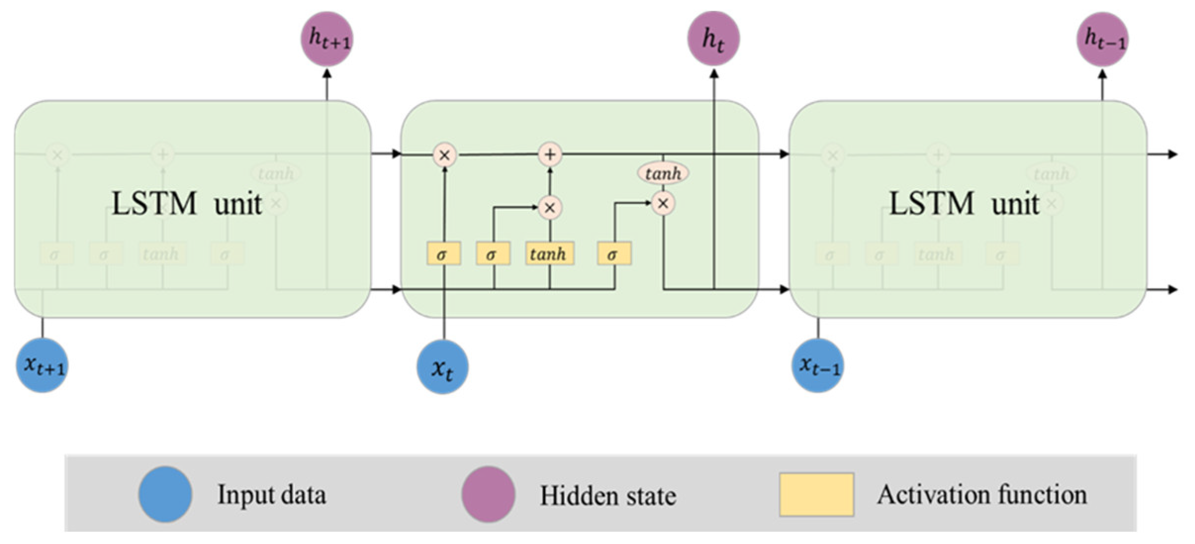
3.2.2. Long Short-Term Memory

Vessel trajectory prediction is a type of time-series prediction task, for which commonly used neural network methods include CNN [45], RNN [30], and LSTM [28]. These three methods have their own features.

(1)

CNN extracts local features from sequence data through convolutional operations, performing well in short-term dependencies but struggling to capture long-term dependencies.

(2)

RNN processes sequential data through recurrent structures, but it is prone to gradient vanishing or exploding problems on long sequences, making it difficult to capture long-term dependencies.

(3)

LSTM is a special type of RNN designed to address the issues of vanishing or exploding gradients encountered by standard RNNs when processing long sequence data [28].

Due to the strong temporal correlation between the spatial features of vessel trajectory data, this paper adopts the LSTM model to process such data. Figure 5 illustrates the unit structure of LSTM, which regulates the flow of information by introducing three gate structures: the forget gate ($f_t$), input gate ($i_t$), and output gate ($o_t$). These gates enable the network to selectively retain and update information over longer time intervals, thereby effectively capturing long-term dependencies.

In the proposed GAT-LSTM model, the essence of GAT is a special feature transformation of nodes in the graph, defined as $\mathcal{F}$: $\mathcal{F}\left(W,h,a,A\right)=h^{\prime }$, where the hidden layer output $h_t$ can be computed given the known data $x_t$ and cell output state $c_t$.

$$\begin{array}{c}{i}_t=\sigma \left(\mathcal{F}\left(W_{x_i},x_t,a,A\right)+\mathcal{F}\left(W_{h_i},h_{t-1},a,A\right)+b_i\right)\end{array}$$

(8)

$$\begin{array}{c}{f}_t=\sigma \left(\mathcal{F}\left(W_{x_f},x_t,a,A\right)+\mathcal{F}\left(W_{h_f},h_{t-1},a,A\right)+b_f\right)\end{array}$$

(9)

$$\begin{array}{c}{o}_t=\sigma \left(\mathcal{F}\left(W_{x_o},x_t,a,A\right)+\mathcal{F}\left(W_{h_o},h_{t-1},a,A\right)+b_o\right)\end{array}$$

(10)

where $i_t$, $f_t$, and $o_t$ are the activation vectors for the input gate, forget gate, and output gate, respectively. W denotes the weight matrix, $h_{t-1}$ is the hidden state of the previous time step, $x_t$ is the input of the current time step, b is the bias vector, and $\sigma$ represents the sigmoid activation function, used to map variables to the range [0, 1]. The input gate determines how much of the candidate hidden state should be added to the cell state at the current time step. The candidate hidden state can be represented by the following equation:

$$\begin{array}{c}{g}_t=tanh\left(\mathcal{F}\left(W_{x_g},x_t,a,A\right)+\mathcal{F}\left(W_{h_g},h_{t-1},a,A\right)+b_g\right)\end{array}$$

(11)

where $g_t$ is the candidate hidden state used to update the cell state, and tanh represents the hyperbolic tangent function used to map variables between [−1, 1]. The cell state is given by Equation (12):

$$\begin{array}{c}{c}_t=f_t\ast c_{t-1}+i_t\ast g_t\end{array}$$

(12)

where $c_t$ represents the cell state, serving as a storage unit for information over time, and * represents element-wise multiplication. The forget gate determines which information should be forgotten or retained, and the output gate decides which information is updated into the cell state. The hidden state at the current time step ($h_t$) can be calculated according to Equation (13):

$$\begin{array}{c}{h}_t=o_t\ast \tanh \left(c_t\right)\end{array}$$

(13)

Through these gate structures, LSTM is able to maintain and update a long-term internal state $c_t$, enabling it to remember both important information from the past and forget less relevant details. In the input transition phase of the state, the GAT-LSTM model particularly considers the influence of graph structure, that is, spatial information. During the transition process between states, the model will simultaneously integrate the temporal and spatial dimensions of correlation. This design enables the GAT-LSTM to fully utilize the spatial relationships between vessels and their temporal changes when processing vessel trajectory prediction, thereby enabling more accurate predictions of future trajectories.

4. Empirical Study

4.1. Data Collection and Preprocessing

To substantiate the efficacy of the proposed model in predicting vessel trajectories, this paper undertakes an exhaustive training and assessment regimen utilizing authentic AIS data. The AIS data, which span latitudes from 23°59.612′ N to 24°35.543′ N and longitudes from 118°0.534′ E to 118°53.297′ E in the vicinity of Xiamen Port from 1 August to 31 August 2020, are procured. The data are utilized to acquire the historical trajectory data of vessels within the specified maritime region, as depicted in Figure 6.

The AIS data encompass a variety of information, including the Maritime Mobile Service Identity (MMSI, a unique vessel identifier), timestamp (BaseDataTime), latitude (LAT), longitude (LON), speed over ground (SOG), course over ground (COG), vessel type, and dimensions such as vessel length and width. AIS data are crucial for maritime navigation and predicting ship trajectories. They provide real-time updates on vessel positions and movements. By monitoring attributes such as LAT, LON, SOG, and COG, the model can accurately estimate the vessel’s future path and facilitate informed decisions for navigation and safety. Notably, dynamic attributes like LON, LAT, SOG, and COG are the most reliable and frequently refreshed data points, with their quality being pivotal to the precision of the model’s predictions. To ensure optimal model performance and to expedite the training process, this study selectively extracts LAT, LON, SOG, and COG as features for the vessel trajectory prediction task. This selection is informed by the recognized positive correlation between the model’s training duration and the number of features incorporated into the model.

The dynamic information within AIS data is updated in real time via sensors integrated with AIS equipment. The acquisition of ship AIS data entails several stages, including generation, encapsulation, reception, and decoding. Communication and environmental factors can cause issues such as signal loss or sensor malfunctions, leading to data duplication, inaccuracies, and omissions within the dynamic information dataset. Therefore, in order to mitigate the detrimental impact of anomalous data on model training, it is imperative to preprocess AIS data prior to its utilization for analysis.

The typical data preprocessing workflow encompasses several key steps: data cleaning and filtering, data interpolation, data standardization, and sampling data by sliding windows. The detailed description of each step is presented as follows, and Figure 7 illustrates the comprehensive procedure for AIS data preprocessing.

Step 1: Data cleaning and filtering

This step involves the removal of incomplete and anomalous data including: ship data where the MMSI is not a 9-digit value, entries with missing values, inconsistent data on vessel dimensions (e.g., vessel width greater than length), and duplicate data where every attribute value matches with one entry. In this paper, the LAT range for ship trajectory positions is set between [23.99° N, 24.60° N], the LON range is set between [118.0° E, 118.89° E], the SOG range is set between [1.5 kt, 25 kt], and the COG range is set between [0°, 360°]. Any data falling outside these specified ranges, as well as records from ships with fewer than 10 data points, will be systematically excluded.

Step 2: Data Interpolation

In trajectory sequences, the time interval between any two adjacent positions may not be fixed. To synchronize AIS data effectively, interpolation is necessary when the interval between adjacent trajectory points of the same vessel exceeds one minute, ensuring that the interpolated timestamps are spaced one minute apart. To make the interpolated trajectory smoother and adhere to vessel navigation habits, the missing values of LAT and LON are interpolated using cubic spline interpolation, as described in Equation (14). Additionally, since the SOG and COG of a vessel tend to be relatively stable over short periods, linear interpolation is used to supplement missing SOG and COG data, as shown in Equation (15):

$$\begin{array}{c}{S}_i\left(t\right)=a_i+b_i\left(t-t_i\right)+c_i{\left(t-t_i\right)}^2+d_i{\left(t-t_i\right)}^3\end{array}$$

(14)

Here, t lies within the interval [$t_i,t_{i+1}$], where $t_i$, $t$, and $t_{i+1}$, respectively, represent the timestamps at the i-th moment, the moment to be interpolated, and the i+1-th moment in the trajectory sequence. The coefficient $a_i,b_i,c_i$, and $d_i$ are determined based on boundary conditions and smoothness requirements.

$$\begin{array}{c}y=y_0+{\displaystyle \frac{\left(y_1-y_0\right)}{\left(x_1-x_0\right)}}\times \left(x-x_0\right)\end{array}$$

(15)

where $x_0$ and $x_1$ are two adjacent time points, $y_0$ and $y_1$ are the ship attribute (SOG or COG) at these two time points, $x$ is the time point that needs interpolation, and $y$ is the corresponding attribute value after interpolation.

Step 3: Data Standardization

To facilitate the convergence of model training, each attribute in the vessel trajectory dataset is standardized based on Equation (16):

$$\begin{array}{c}\tilde{x}={\displaystyle \frac{x-\overline{x}\left(x_{data}\right)}{s\left(x_{data}\right)}}\end{array}$$

(16)

where x represents the attribute value of the vessel, $\overline{x}(·)$ represents the mean of the corresponding attribute in the dataset, $s(·)$ is the standard deviation of the corresponding attribute in the dataset, and $\tilde{x}$ is the standardized value of the corresponding vessel attribute.

Step 4: Sampling data by sliding windows

The continuity and temporality of the data are closely connected to the model performance in understanding and predicting the dynamic changes in ship trajectories. In this research, a sliding window sampling technique is employed to effectively extract data samples from the corrected trajectory sequences in order to ensure the continuity and temporality of the data.

To be specific, the length of the sliding window is set first based on the input sequence length (m) and the predicted output sequence length (n), resulting in a data length of (m + n) for each sliding window. Starting from the beginning of the sequence, the sliding window progressively moves along the time axis with the shift of one time unit at each step, until it covers the entire sequence. In this way, the data within each window are used as an independent sample for model training, ensuring that the model can learn trajectory characteristics at different time points.

Finally, after preprocessing, the trajectory dataset of 1562 vessels in the waters of Xiamen Port are obtained, including 2,236,324 AIS data points. These data are randomly divided into three subsets, with 60% used as the model training set, 20% as the validation set, and the remaining 20% as the testing set.

4.2. Baseline Methods and Evaluation Criteria

To verify its effectiveness, the proposed ship trajectory prediction model based on GAT-LSTM will be compared with traditional baseline models. These compared trajectory prediction methods are described as follows:

LSTM: As a specialized type of recurrent neural network architecture, LSTM is mainly controlled through three gates: the forget gate determines which previous information to discard, the input gate is responsible for incorporating as much new information as possible, and the output gate decides what information to output. It overcomes the problem of vanishing or exploding gradients and is better at capturing both long-term and short-term information for sequence prediction [29].

CNN-LSTM: CNN-LSTM is a deep-learning architecture designed for modelling and predicting the trajectory by incorporating both the strengths of the CNN and LSTM. The CNN layer is first used to extract the spatial structure of the data, effectively identifying patterns and features at different levels. The extracted information is then passed to the LSTM layer, which specializes in capturing long-term sequence correlations. This synergistic integration makes it exceptionally suited for tasks requiring an understanding of both the spatial and temporal dimensions together [46].

GRU: GRU is a variant of LSTM where a single reset gate replaces the forget gate and input gate of LSTM, and the update operation of unit states becomes an update gate, making the structure simpler. These mechanisms enable the GRU to selectively update and reset its hidden states, effectively capturing long-term dependencies while alleviating the vanishing gradient problem [47].

Seq2seq: This is a sequence-based trajectory prediction model composed of an encoder–decoder framework. It is designed to handle variable-length input sequences and generate variable-length output sequences. The encoder reads the input sequence and generates a fixed-size representation to capture its semantics, while the decoder generates the output sequence based on this representation [29].

In this paper, the mean absolute error (MAE), root mean square error (RMSE), average displacement error (ADE), and final displacement error (FDE) are used as evaluation metrics to quantitatively evaluate the accuracy of ship trajectory prediction results [48,49]. Smaller values of these metrics indicate a higher precision in the trajectory prediction of the corresponding model. The calculation equations are as follows:

$$\begin{array}{c}MAE={\displaystyle \frac{1}{n}}{\displaystyle \sum _{i=1}^n}\left|Y_i-\widehat{Y_i}\right|\end{array}$$

(17)

$$\begin{array}{c}RMSE=\sqrt{{\displaystyle \frac{1}{n}}{\displaystyle \sum _{i=1}^n}{\left(Y_i-\widehat{Y_i}\right)}^2}\end{array}$$

(18)

$$\begin{array}{c}ADE={\displaystyle \frac{1}{n}}{\displaystyle \sum _{i=1}^n}\sqrt{{{(x}_i-\widehat{x_i})}^2+{{(y}_i-\widehat{y_i})}^2}\end{array}$$

(19)

$$\begin{array}{c}FDE=\sqrt{{{(x}_f-\widehat{x_f})}^2+{{(y}_f-\widehat{y_f})}^2}\end{array}$$

(20)

where $\widehat{Y_i}$ is the predicted value of the i-th sample, $Y_i$ is the true value of the i-th sample, and n represents the number of samples. ($\widehat{x_i},\widehat{y_i})$ is the predicted position (latitude and longitude) of the i-th sample, ($x_i,y_i$) is the corresponding true value of the i-th sample, ($\widehat{x_f},\widehat{y_f})$ is the predicted position of the final trajectory point, and ($x_f,y_f$) is the corresponding true value of the final trajectory point.

4.3. Parameter Setting and Implementation Detail

In this section, we outline the parameters of the GAT-LSTM model proposed in this paper. The vessel trajectory data were segmented into three distinct subsets: a training set, a testing set, and a validation set. The model leverages features from 20 consecutive frames of ship trajectory sequences as inputs to forecast the trajectory sequence for the subsequent 10 frames. Additionally, the input features are four-dimensional, encompassing the longitude, latitude, speed over ground, and course over ground.

Throughout the training process, the batch size was set to 32, and the Adam optimizer [50] with an initial learning rate of 0.0001 was employed to incrementally update the neural network weights of the model. A dropout ratio of 0.3 was implemented to regularize the embedding sequence, with each iteration requiring approximately 75–82 s. Through this training regimen, a total of 88,340 trainable parameters were established. The results indicate that the loss value per epoch progressively diminishes with each iteration, culminating in convergence, as depicted in Figure 8.

All experiments were executed under identical hardware conditions using a laptop equipped with an Intel Core i5-8265U [email protected] GHz and an NVIDIA GeForce MX150 GPU. The software environment was also consistent, featuring the Windows 10 operating system and the deep-learning framework TensorFlow.

4.4. Experimaental Results and Analysis

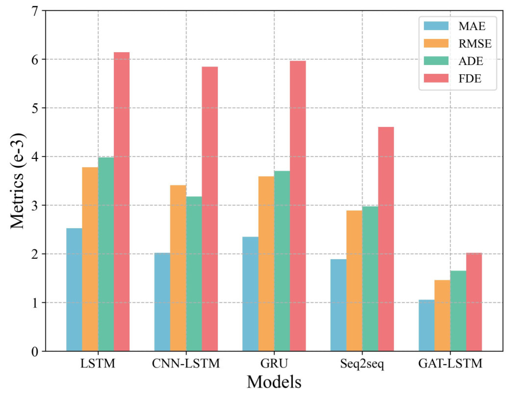
To qualitatively assess the efficacy of the model introduced in this paper, this section employs the aforementioned dataset to train both the baseline models and the proposed model. Figure 9 illustrates the evolution of the loss functions across various models throughout the training phase, with (a) through (e) representing the loss curves for the LSTM, CNN-LSTM, Seq2seq, GRU, and GAT-LSTM models, respectively. From these figures, it can be observed that the loss value progressively stabilizes with an increasing number of epochs, indicating that the models are achieving a state of convergence.

Subsequently, to validate the predictive capabilities of the proposed models, typical navigation scenarios that are considered as the most common and critical operations in maritime navigation were selected from the previous research [51,52,53], including straightforward navigation, emergency turns, turning operations in open waters, turning near an anchorage, and navigation in narrow waterways. To be specific, (1) straight sailing and turning maneuvers account for the majority of the time during a ship’s entire navigation process, thus testing the basic performance of the proposed model; (2) navigation in narrow or intricate waterways could verify the applicability of the proposed models in complex environments; and (3) infrequent emergency avoidance and deceleration could evaluate the responsiveness and predictive accuracy of the models. Therefore, incorporating these typical scenarios into the evaluation helps support the validity and practical relevance of the research findings. Figure 10 visualized the results of the scenario analysis.

As shown in Figure 10a,b, when the vessel is sailing in the same direction, meaning its trajectory is straight, the prediction outcomes of the models show minimal variation, with both the baseline and GAT-LSTM models achieving relatively accurate results. However, as the vessel begin to turn or prepare for a turn, the difference in prediction accuracy between the baseline and proposed models gradually becomes apparent.

Figure 10c shows the trajectory prediction results when the vessel turns after sailing straight for a period and then quickly returns to a straight course. The predicted trajectories from the LSTM, CNN-LSTM, and GRU models deviate significantly from the actual trajectory (the ‘Ground Truth’ in the figure). In contrast, the Seq2seq and GAT-LSTM models’ predictions follow the same trend as the actual trajectory, but the prediction values of the Seq2seq model deviates significantly from the true values, especially at the last trajectory point. Meanwhile, the GAT-LSTM model provides predictions that are much closer to the actual values under such circumstances.

Figure 10d presents the predictive outcomes for a vessel’s trajectory after making a turn in open waters. It can be seen that all baseline models predict ship trajectories that are almost straight lines, which is inconsistent with the true turning trajectory. Conversely, the proposed GAT-LSTM model accurately predicts both the directional trend and positional shifts in ship movement due to its robust spatio-temporal modelling capability. The difference in prediction accuracy is likely due to the fact that vessels need to execute evasive maneuvers to avoid potential conflicts with nearby sailing vessels. Trained solely on historical trajectory data, these baseline models fail to consider the impacts of other vessels on the movement of the target vessel in this scenario, thus resulting in unsatisfactory predictions.

Figure 10e displays the trajectory predictions as the vessel turns towards an anchorage. Here, it is apparent that the GAT-LSTM model outperforms its counterparts, offering predictions that most closely align with the vessel’s actual trajectory. The time interval between adjacent points in the real ship trajectory is the same, but the distance between the two points is decreasing, indicating that the ship is in a deceleration state. The baseline models are not able to present this detail effectively.

Figure 10f shows trajectory predictions in a narrow channel after a turn, and, while all models reasonably forecast the vessel’s navigational trend, the prediction results of the proposed model are the closest to the true values compared to other models.

Overall, the outcomes illustrated in Figure 10 clarify the prediction performances of these models, which are summarized as follows:

(1)

The LSTM and GRU models perform poorly compared to other comparative models, with their predictions exhibiting significant deviations for most segments and only aligning with the actual values of certain trajectory segments.

(2)

The prediction results of the CNN-LSTM and Seq2seq models are roughly similar, and both models show a relatively good prediction performance in most trajectory segments. However, in some cases, although they can provide satisfactory results in the early stages of trajectory prediction, the accuracy of the prediction gradually decreases over time. This phenomenon may be due to the difficulty of these models in capturing small changes and complex details in trajectories when dealing with highly dynamic scenes.

(3)

The predicted trajectory of the GAT-LSTM model is closest to the real trajectory. This is probably because the model combines the capabilities of spatial relationships and time-series prediction, and can capture complex interactions between ships through a graph attention mechanism. When vessels perform complex actions, such as turning, it can also understand the nonlinearity of the vessel behavior well, demonstrating the accuracy and robustness of the model.

Further, a quantitative analysis is conducted to test the performance of the baseline models and the proposed model. Metrics are used to compare the predictive performance of five different models including MAE, RMSE, ADE, and FDE. Consequently,

Table 1. Quantitative analysis results of predictive performance of different models.

Metric	Models
	LSTM	CNN-LSTM	GRU	Seq2seq	GAT-LSTM
MAE	2.526 $\times$ 10−3	2.021 $\times$ 10−3	2.350 $\times$ 10−3	1.890 $\times$ 10−3	1.057 $\times$ 10−3
RMSE	3.778 $\times$ 10−3	3.411 $\times$ 10−3	3.592 $\times$ 10−3	2.891 $\times$ 10−3	1.461 $\times$ 10−3
ADE	3.978 $\times$ 10−3	3.175 $\times$ 10−3	3.704 $\times$ 10−3	2.974 $\times$ 10−3	1.650 $\times$ 10−3
FDE	6.143 $\times$ 10−3	5.844 $\times$ 10−3	5.963 $\times$ 10−3	4.607 $\times$ 10−3	2.018 $\times$ 10−3

provides the prediction error assessment results for each model and Figure 11 presents the result differences between these models more visually.

From the results of the vessel trajectory prediction models, it can be seen that the predicted trajectory of the GAT-LSTM model is closer to the real trajectory, which is consistent with the metric evaluation results in Table 1. This highlights the importance of considering the spatio-temporal correlation and vessel interaction in the prediction task. From the table, it is evident that the GAT-LSTM has the smallest MAE and RMSE, which are (1.057 × 10⁻³, 1.461 × 10⁻³), and the prediction errors are about (58.16%, 61.33%) lower than the LSTM model, about (47.70%, 57.17%) lower than the CNN-LSTM model, about (55.02%, 59.33%) lower than the GRU model, and about (44.07%, 49.46%) lower than the Seq2seq model, respectively. Similarly, GAT-LSTM also has the smallest ADE and FDE, which are (1.650 × 10⁻³, 2.018 × 10⁻³), which are about (58.52%, 67.15%) lower than the LSTM model, about (48.03%, 65.47%) lower than the CNN-LSTM model, about (55.45%, 66.16%) lower than the GRU model, and about (44.52%, 56.20%) lower than the Seq2seq model, respectively. The above results indicate that the proposed model has an excellent predictive performance in vessel trajectory prediction.

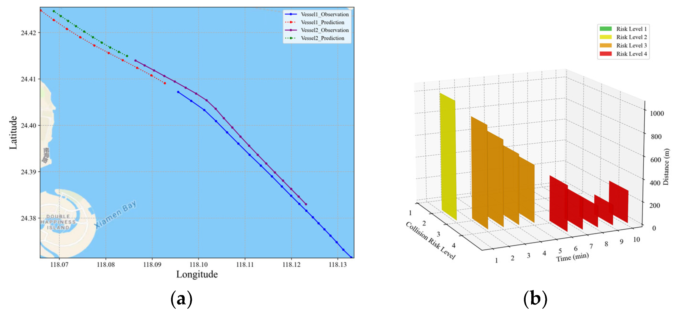
4.5. Practical Implication

The GAT-LSTM vessel trajectory prediction method proposed in this paper can accurately predict the future navigation routes of vessels and significantly enhance navigation safety. In order to deeply explore the specific effects and guiding significance of this method in practical applications for ports, governments, and crew members in maintaining vessel navigation safety, this study selected two typical scenarios with potential risks: head-on and overtaking, for detailed analysis. Through the analysis of these practical cases, this paper verifies the effectiveness and practical value of the proposed trajectory prediction method. The data used in the case study are all sourced from real vessel navigation records, with the MMSI numbers and types of the vessels involved detailed in

Table 2. Vessel information in case study.

	MMSI of Vessel 1 (Own Vessel)	Vessel Type	MMSI of Vessel 2 (Target Vessel)	Vessel Type
Head-on	351297000	Container vessel	412473290	Container vessel
Overtaking	477958800	Container vessel	538006763	tanker

.

Figure 12a shows the trajectory prediction results based on the GAT-LSTM model when two vessels are in a head-on situation. The input to the model includes the observation trajectories of vessel 1 (blue solid line) and vessel 2 (purple solid line) over the previous 20 min, and the model outputs the predicted trajectories for the next 10 min of vessel 1 (red dashed line) and vessel 2 (green dashed line), respectively. During this period, it can be observed that the two vessels gradually approach and then begin to move away. To quantify this process, the study employs the haversine distance $D_t$ to represent the distance between two vessels at any future time t, which serves as a metric to assess the risk of collision between them. In addition, to clearly demonstrate the evolution of risk, vessel risk based on haversine distance is categorized into four levels: {Risk level 1: $D_t>2\mathrm{k}$; Risk level 2: ${1\mathrm{k}\mathrm{m}<D}_t\le 2\mathrm{k}\mathrm{m}$; Risk level 3: ${500\mathrm{m}<D}_t\le 1\mathrm{k}\mathrm{m}$; Risk level 4: $D_t\le 500\mathrm{m}$}. Figure 12b shows the risk outcomes of the own vessel and the target vessel for the next 10 min in a head-on situation. The proposed prediction method can fully reflect the process of the risk situation gradually changing from stable to urgent and then back to stable when two vessels encounter each other, which is highly consistent with the actual navigation situation. Moreover, the effective conversion between risk levels also indirectly proves the rationality of the proposed method. In Figure 12b, the risk level between the two vessels increases from 3 to 4 between the fifth and sixth minute, indicating they are in a relatively dangerous state. To ensure sufficient time for collision avoidance maneuvers, it is recommended that drivers initiate evasive maneuvers starting at the fourth minute to prevent potential maritime accidents.

Similarly, Figure 13a presents the trajectory prediction results of two vessels in an overtaking situation. It can be observed that the sailing speed of vessel 1 is greater than that of vessel 2, with the distance between them gradually decreasing over time until the last time step, where it increases again. Figure 13b illustrates the risk situation of the own vessel and the target vessel over the next 10 min in the overtaking scenario. The risk level gradually increases with the movement time. Notably, the risk level between the two vessels escalates from Level 3 to Level 4 between the fifth and sixth minutes. This shift can remind the driver to perform collision avoidance operations in a timely manner. The vessel trajectory prediction method introduced in this paper offers a higher accuracy compared to baseline models and can provide effective guidance for collision avoidance in real navigation scenarios by combining trajectory prediction and risk calculation, demonstrating its practical utility.

5. Conclusions

Vessel trajectory prediction is crucial for improving the safety and efficiency of shipping. It helps to effectively plan navigation routes, avoid collision risks, and optimize traffic management and resource planning. Accurate vessel trajectory predictions can support intelligent navigation and ensure safety in waterborne traffic. This paper proposes a model based on GAT and LSTM aimed at enhancing the accuracy of vessel trajectory predictions. The model comprises two modules: the GAT module, which summarizes interaction information among vessels within the vessel network diagram to extract spatial features of vessel trajectories, and the LSTM module, which further extracts temporal features from trajectory data. These features are then integrated to predict the future movement trajectories of vessels. In addition, the predictive performance of the proposed model was evaluated based on real AIS data in different navigation scenarios. The experimental results show that the GAT-LSTM model significantly outperforms baseline models, with a reduction in MAE and RMSE by 44.07% and 49.46%, and a decrease in ADE and FDE by 44.52% and 56.20%, respectively, compared to the optimal baseline model Seq2seq. These results confirm the proposed vessel trajectory prediction method’s ability to achieve a higher prediction accuracy.

In addition to the dynamic features of vessels, static attributes such as the length, width, and draft of a vessel may also be relevant to trajectory prediction. Generally, considering more variables can improve the accuracy of predictions, but it also increases the complexity of the model, prolongs training time, and may lead to the slower convergence speed of the model. Therefore, in future research, we can consider introducing a wider array of features as input parameters for the model and finding a balance to ensure a compromise between the number of features and the training time, thereby improving the reliability of trajectory prediction. In addition, environmental factors can also have an impact on the prediction results. Deep-learning methods can be used to encode environmental factors and input them into the prediction model to consider environmental factors during the prediction process, further improving the accuracy of the predictions. In the practical implication section of this paper, the haversine distance between vessels is used as a metric to measure risk, but this method may not be accurate enough. Future research could consider incorporating the Distance at Closest Point of Approach (DCPA) and Time to Closest Point of Approach (TCPA) to adopt more reasonable evaluation metrics.

References

1. Yang, Z.S.; Wan, C.P.; Yang, Z.L.; Yin, J.B.; Yu, Q. A machine learning-based Bayesian model for predicting the duration of ship detention in PSC inspection. Transp. Res. Part E Logist. Transp. Rev. 2023, 180, 103331. [Google Scholar] [CrossRef]
2. Chen, X.; Wu, H.; Han, B.; Liu, W.; Montewka, J.; Liu, W. Orientation-aware ship detection via a rotation feature decoupling supported deep learning approach. Ocean Eng. 2023, 125, 106686. [Google Scholar] [CrossRef]
3. UNCTAD. Review of Maritime Transport 2023; United Nations Publications: New York, NY, USA, 2024. [Google Scholar]
4. Yu, Q.; Teixeira, A.; Liu, K.; Rong, H.; Soares, C. An integrated dynamic ship risk model based on Bayesian Networks and Evidential Reasoning. Reliab. Eng. Syst. Saf. 2021, 216, 107993. [Google Scholar] [CrossRef]
5. Kaptan, M.; Uğurlu, Ö.; Wang, J. The effect of nonconformities encountered in the use of technology on the occurrence of collision, contact and grounding accidents. Reliab. Eng. Syst. Saf. 2021, 215, 107886. [Google Scholar] [CrossRef]
6. Guo, S.; Zhang, H.; Guo, Y. Toward Multimodal Vessel Trajectory Prediction by modeling the distribution of modes. Ocean Eng. 2023, 282, 115020. [Google Scholar] [CrossRef]
7. Chen, X.Q.; Dou, S.T.; Song, T.Q.; Wu, H.F.; Sun, Y.; Xian, J.F. Spatial-Temporal Ship Pollution Distribution Exploitation and Harbor Environmental Impact Analysis via Large-Scale AIS Data. J. Mar. Sci. Eng. 2024, 12, 960. [Google Scholar] [CrossRef]
8. Zhang, X.; Liu, J.; Gong, P.; Chen, C.; Han, B.; Wu, Z. Trajectory prediction of seagoing ships in dynamic traffic scenes via a gated spatio-temporal graph aggregation network. Ocean Eng. 2023, 287, 115886. [Google Scholar] [CrossRef]
9. Tong, X.; Chen, X.; Sang, L.; Mao, Z.; Wu, Q. Vessel trajectory prediction in curving channel of inland river. In Proceedings of the 2015 International Conference on Transportation Information and Safety (ICTIS), Wuhan, China, 25–28 June 2015; pp. 706–714. [Google Scholar] [CrossRef]
10. Gutierrez, L.A.; Kun, J.I.N.; Gutierrez, L.A. Trajectory Prediction Algorithm Based on Gaussian Mixture Model. J. Softw. 2015, 26, 1048–1063. [Google Scholar] [CrossRef]
11. Cheng, Q.; Wang, C. A Method of Trajectory Prediction Based on Kalman Filtering Algorithm and Support Vector Machine Algorithm. In Proceedings of 2017 Chinese Intelligent Systems Conference: Volume I; Springer: Singapore, 2018. [Google Scholar]
12. Chen, P.; Yang, F.; Mou, J.; Chen, L.; Li, M. Regional ship behavior and trajectory prediction for maritime traffic management: A social generative adversarial network approach. Ocean Eng. 2024, 299, 117186. [Google Scholar] [CrossRef]
13. Jaskólski, K. Automatic Identification System (AIS) Dynamic Data Estimation Based on Discrete Kalman Filter (KF) Algorithm. Sci. J. Pol. Nav. Acad. 2017, 211, 71–87. [Google Scholar] [CrossRef]
14. Fossen, S.; Fossen, T.I. Extended kalman filter design and motion prediction of ships using live automatic identification system (AIS) Data. In Proceedings of the 2018 2nd European Conference on Electrical Engineering and Computer Science (EECS), Bern, Switzerland, 20–22 December 2018; pp. 464–470. [Google Scholar] [CrossRef]
15. Mazzarella, F.; Arguedas, V.F.; Vespe, M. Knowledge-based vessel position prediction using historical AIS data. In Proceedings of the 2015 Sensor Data Fusion: Trends, Solutions, Applications (SDF), Bonn, Germany, 6–8 December 2015; pp. 1–6. [Google Scholar] [CrossRef]
16. Perera, L.P.; Oliveira, P.; Soares, C.G. Maritime traffic monitoring based on vessel detection, tracking, state estimation, and trajectory prediction. IEEE Trans. Intell. Transp. Syst. 2012, 13, 1188–1200. [Google Scholar] [CrossRef]
17. Zhou, T.; Jiang, D.; Lin, Z.; Han, G.; Xu, X.; Qin, J. Hybrid dual Kalman filtering model for short-term traffic flow forecasting. IET Intell. Transp. Syst. 2019, 13, 1023–1032. [Google Scholar] [CrossRef]
18. Zhang, X.; Liu, G.; Hu, C.; Ma, X. Wavelet analysis based hidden markov model for large ship trajectory prediction. In Proceedings of the 2019 Chinese Control Conference (CCC), Guangzhou, China, 27–30 July 2019; pp. 2913–2918. [Google Scholar] [CrossRef]
19. Cheng, Y.; Qiao, Y.; Yang, J. An improved Markov method for prediction of user mobility. In Proceedings of the 2016 12th International Conference on Network and Service Management (CNSM), Montreal, QC, Canada, 31 October–4 November 2016; pp. 394–399. [Google Scholar] [CrossRef]
20. Murray, B.; Perera, L.P. A data-driven approach to vessel trajectory prediction for safe autonomous ship operations. In Proceedings of the 2018 Thirteenth International Conference on Digital Information Management (ICDIM), Berlin, Germany, 24–26 September 2018; pp. 240–247. [Google Scholar] [CrossRef]
21. Dalsnes, B.R.; Hexeberg, S.; Flåten, A.L.; Eriksen, B.O.H.; Brekke, E.F. The Neighbor Course Distribution Method with Gaussian Mixture Models for AIS-Based Vessel Trajectory Prediction. In Proceedings of the 2018 21st International Conference on Information Fusion (FUSION), Cambridge, UK, 10–13 July 2018; pp. 580–587. [Google Scholar] [CrossRef]
22. Rong, H.; Teixeira, A.P.; Guedes Soares, C. Ship trajectory uncertainty prediction based on a Gaussian Process model. Ocean Eng. 2019, 182, 499–511. [Google Scholar] [CrossRef]
23. Murray, B.; Perera, L.P. An ais-based multiple trajectory prediction approach for collision avoidance in future vessels. In Proceedings of the ASME 2019 38th International Conference on Ocean, Offshore and Arctic Engineering, Glasgow, Scotland, 9–14 June 2019. [Google Scholar] [CrossRef]
24. Liu, J.; Shi, G.; Zhu, K. Vessel trajectory prediction model based on ais sensor data and adaptive chaos differential evolution support vector regression (ACDE-SVR). Appl. Sci. 2019, 9, 2983. [Google Scholar] [CrossRef]
25. Zhang, C.; Bin, J.; Wang, W.; Peng, X.; Wang, R.; Halldearn, R.; Liu, Z. AIS data driven general vessel destination prediction: A random forest based approach. Transp. Res. Part C Emerg. Technol. 2020, 118, 102729. [Google Scholar] [CrossRef]
26. Nguyen, D.D.; Le Van, C.; Ali, M.I. Demo: Vessel trajectory prediction using sequence-to-sequence models over spatial grid. In Proceedings of the DEBS’18: Proceedings of the 12th ACM International Conference on Distributed and Event-Based Systems, Hamilton, New Zealand, 25–29 June 2018; pp. 258–261. [Google Scholar] [CrossRef]
27. Capobianco, S.; Millefiori, L.M.; Forti, N.; Braca, P.; Willett, P. Deep Learning Methods for Vessel Trajectory Prediction Based on Recurrent Neural Networks. IEEE Trans. Aerosp. Electron. Syst. 2021, 57, 4329–4346. [Google Scholar] [CrossRef]
28. Zhang, Z.; Ni, G.; Xu, Y. Ship Trajectory Prediction based on LSTM Neural Network. In Proceedings of the 2020 IEEE 5th Information Technology and Mechatronics Engineering Conference (ITOEC), Chongqing, China, 12–14 June 2020; pp. 1356–1364. [Google Scholar] [CrossRef]
29. Forti, N.; Millefiori, L.M.; Braca, P.; Willett, P. Prediction of Vessel Trajectories from Ais Data via Sequence-to-Sequence Recurrent Neural Networks. In Proceedings of the ICASSP 2020—2020 IEEE International Conference on Acoustics, Speech and Signal Processing (ICASSP), Barcelona, Spain, 4–8 May 2020; pp. 8931–8935. [Google Scholar]
30. Suo, Y.; Chen, W.; Claramunt, C.; Yang, S. A ship trajectory prediction framework based on a recurrent neural network. Sensors 2020, 20, 5133. [Google Scholar] [CrossRef]
31. Liu, C.; Li, Y.; Jiang, R.; Du, Y.; Lu, Q. TPR-DTVN: A Routing Algorithm in Delay Tolerant Vessel Network Based on Long-Term Trajectory Prediction. Wirel. Commun. Mob. Comput. 2021, 2021, 6630265. [Google Scholar] [CrossRef]
32. Ghaffarian, S.; Valente, J.; Van Der Voort, M.; Tekinerdogan, B. Effect of attention mechanism in deep learning-based remote sensing image processing: A systematic literature review. Remote Sens. 2021, 13, 2965. [Google Scholar] [CrossRef]
33. Jia, H.; Yang, Y.; An, J.; Fu, R. A Ship Trajectory Prediction Model Based on Attention-BILSTM Optimized by the Whale Optimization Algorithm. Appl. Sci. 2023, 13, 4907. [Google Scholar] [CrossRef]
34. Zhang, T.; Zheng, X.Q.; Liu, M.X. Multiscale attention-based LSTM for ship motion prediction. Ocean Eng. 2021, 230, 109066. [Google Scholar] [CrossRef]
35. Zhao, L.; Zuo, Y.; Li, T.; Chen, C.L.P. Application of an Encoder–Decoder Model with Attention Mechanism for Trajectory Prediction Based on AIS Data: Case Studies from the Yangtze River of China and the Eastern Coast of the U.S. J. Mar. Sci. Eng. 2023, 11, 1530. [Google Scholar] [CrossRef]
36. Zhang, X.; Fu, X.; Xiao, Z.; Xu, H.; Qin, Z. Vessel Trajectory Prediction in Maritime Transportation: Current Approaches and beyond. IEEE Trans. Intell. Transp. Syst. 2022, 23, 19980–19998. [Google Scholar] [CrossRef]
37. Wang, S.; Li, Y.; Zhang, Z.; Xing, H. Big data driven vessel trajectory prediction based on sparse multi-graph convolutional hybrid network with spatio-temporal awareness. Ocean Eng. 2023, 287, 115695. [Google Scholar] [CrossRef]
38. Feng, H.; Cao, G.; Xu, H.; Ge, S.S. IS-STGCNN: An Improved Social spatial-temporal graph convolutional neural network for ship trajectory prediction. Ocean Eng. 2022, 266, 112960. [Google Scholar] [CrossRef]
39. Liu, R.W.; Zheng, W.; Liang, M. Spatio-temporal multi-graph transformer network for joint prediction of multiple vessel trajectories. Eng. Appl. Artif. Intell. 2024, 129, 107625. [Google Scholar] [CrossRef]
40. Liu, R.W.; Liang, M.; Nie, J.; Yuan, Y.; Xiong, Z.; Yu, H.; Guizani, N. STMGCN: Mobile Edge Computing-Empowered Vessel Trajectory Prediction Using Spatio-Temporal Multigraph Convolutional Network. IEEE Trans. Ind. Inform. 2022, 18, 7977–7987. [Google Scholar] [CrossRef]
41. Zhao, J.; Yan, Z.; Zhou, Z.Z.; Chen, X.; Wu, B.; Wang, S. A ship trajectory prediction method based on GAT and LSTM. Ocean Eng. 2023, 289, 116159. [Google Scholar] [CrossRef]
42. Li, H.; Jiao, H.; Yang, Z. Ship trajectory prediction based on machine learning and deep learning: A systematic review and methods analysis. Eng. Appl. Artif. Intell. 2023, 126, 107062. [Google Scholar] [CrossRef]
43. Wang, S.; Li, Y.; Xing, H.; Zhang, Z. Vessel trajectory prediction based on spatio-temporal graph convolutional network for complex and crowded sea areas. Ocean Eng. 2024, 298, 117232. [Google Scholar] [CrossRef]
44. Xia, Z.; Zhang, Y.; Yang, J.; Xie, L. Dynamic spatial–temporal graph convolutional recurrent networks for traffic flow forecasting. Expert Syst. Appl. 2024, 240, 122381. [Google Scholar] [CrossRef]
45. Liu, W.; Cao, Y.; Guan, M.; Liu, L. Research on Ship Trajectory Prediction Method based on CNN-RGRU-Attention Fusion Model. IEEE Access. 2024, 12, 63950–63957. [Google Scholar] [CrossRef]
46. Lee, H.J.; Park, D.J. Collision evasive action timing for MASS using CNN–LSTM-based ship trajectory prediction in restricted area. Ocean Eng. 2024, 294, 116766. [Google Scholar] [CrossRef]
47. Adege, A.B.; Lin, H.P.; Wang, L.C. Mobility Predictions for IoT Devices Using Gated Recurrent Unit Network. IEEE Internet Things J. 2020, 7, 505–517. [Google Scholar] [CrossRef]
48. Huang, Z.; Wang, Z.; Chen, H.; Zhang, Z.; Wang, J.; Yuan, Z.; Jin, Y.; Wu, X. EA-VTP: Environment-Aware Long-Term Vessel Trajectory Prediction. In Proceedings of the 2022 International Joint Conference on Neural Networks (IJCNN), Padua, Italy, 18–23 July 2022; pp. 1–7. [Google Scholar] [CrossRef]
49. Li, J.; Yang, L.; Chen, Y.; Jin, Y. MFAN: Mixing Feature Attention Network for trajectory prediction. Pattern Recognit. 2024, 146, 109997. [Google Scholar] [CrossRef]
50. Kingma, D.P.; Ba, J.L. Adam: A method for stochastic optimization. In Proceedings of the 3rd International Conference on Learning Representations, ICLR 2015, San Diego, CA, USA, 7–9 May 2015; pp. 1–15. [Google Scholar]
51. Li, H.; Jiao, H.; Yang, Z. AIS data-driven ship trajectory prediction modelling and analysis based on machine learning and deep learning methods. Transp. Res. Part E Logist. Transp. Rev. 2023, 175, 103152. [Google Scholar] [CrossRef]
52. Liu, R.W.; Liang, M.; Nie, J.; Lim, W.Y.B.; Zhang, Y.; Guizani, M. Deep Learning-Powered Vessel Trajectory Prediction for Improving Smart Traffic Services in Maritime Internet of Things. IEEE Trans. Netw. Sci. Eng. 2022, 9, 3080–3094. [Google Scholar] [CrossRef]
53. Shin, Y.; Kim, N.; Lee, H.; In, S.Y.; Hansen, M.; Yoon, Y. Deep learning framework for vessel trajectory prediction using auxiliary tasks and convolutional networks. Eng. Appl. Artif. Intell. 2024, 132, 107936. [Google Scholar] [CrossRef]
Figure 1. Vessel interaction networks.
Jmse 12 01351 g001
Figure 2. The schematic diagram of the adjacency matrix.
Jmse 12 01351 g002
Figure 3. The overall structural framework of the GAT-LSTM model.
Jmse 12 01351 g003
Figure 4. The structure of graph attention network. (a) Calculation of attention coefficient between node i and node j. (b) A diagram of a multi-head (K = 3) attention layer, with arrows of different colors representing independent attention calculations. The features of each head are concatenated to obtain h 1 .
Jmse 12 01351 g004
Figure 5. The unit structure of long short-term memory.
Jmse 12 01351 g005
Figure 6. The visualization of vessel trajectories in research waters.
Jmse 12 01351 g006
Figure 7. The overall process of AIS data preprocessing.
Jmse 12 01351 g007
Figure 8. Training procedure of the proposed model.
Jmse 12 01351 g008
Figure 9. The loss curves of the baseline model and the proposed model. (a) LSTM model loss curve. (b) CNN-LSTM model loss curve. (c) GRU model loss curve. (d) Seq2seq model loss curve. (e) GAT-LSTM model loss curve.
Jmse 12 01351 g009
Figure 10. Visualization results of vessel trajectory prediction models under different navigation scenarios. (a,b) The trajectory prediction results of vessel sailing in the same direction. (c) The trajectory prediction results when the vessel turns after sailing straight for a period and then quickly returns to a straight course. (d) The trajectory prediction results of vessel after turning in open waters. (e) The trajectory prediction results as the vessel turns towards an anchorage. (f) The trajectory prediction results in a narrow channel after a turn.
Jmse 12 01351 g010
Figure 11. Comparison of predictive performance between baseline models and proposed model.
Jmse 12 01351 g011
Figure 12. (a) The vessel trajectory prediction results of the head-on situation. (b) The risk result of the head-on situation.
Jmse 12 01351 g012
Figure 13. (a) The vessel trajectory prediction results of the overtaking situation. (b) The risk result of the overtaking situation.
Jmse 12 01351 g013