Numerical Simulation of Bionic Underwater Vehicle Morphology Drag Optimisation and Flow Field Noise Analysis

Abstract

The study of aquatic organisms’ ectomorphology is important to understanding the mechanisms of efficient swimming and drag reduction in fish. The drag reduction mechanism in fish remains unknown yet is needed for optimising the efficiency of bionic fish. It is thus crucial to conduct drag tests and analyses. In this paper, an optimal dolphin morphological model is constructed taking the beakless porpoise as the research object. A numerical simulation of the dolphin body model is carried out for different combinations of pitch angle and speed adopting computational fluid dynamics, and the flow field noise of the dolphin body model is solved for different speeds using the FW-H equation. When the dolphin model is oriented horizontally, the differential pressure drag accounts for approximately 20–25% of the total drag as airspeed increases. As both the pitch angle and airspeed increase, the differential pressure drag and friction drag decrease with increasing airspeed. Moreover, the acoustic energy is mainly concentrated at low frequencies for both the dolphin and Bluefin-21 models. The dolphin body model has better noise performance than the Bluefin-21 model at the same speed. The optimisation of the external morphology of the bionic underwater submarine and the analysis of the shape drag are thus important for revealing the drag reduction mechanism, reducing noise in the flow field and provide guidance for research on bionic fish.

1. Introduction

With continuous advances in science and technology, underwater vehicles are playing an increasingly important role in the investigation of pelagic fishery resources [1]. In particular, highly bionic robotic fish, designed to imitate the movements and appearance of real fish, have better diving performance and adaptability, and they are thus suited to tasks such as pelagic environment monitoring and pelagic biology research [2]. Research on underwater vehicles has focused on the profile resistance problem, with the magnitude of resistance directly affecting the energy consumption and performance of underwater vehicles [3].

The flow noise generated by an underwater vehicle in operation mainly originates from the vortices and turbulence generated by the interaction between the hull surface and water flow. Reducing the profile resistance can therefore reduce the formation of eddies and turbulence and thus the generation of flow noise.

Du Xiangpang et al. [4] conducted water hole data experiments and calculations and confirmed that an optimised shape is important to drag reduction. Kou Guanyuan et al. [5] designed a submarine shape with an optimal hydrodynamic coefficient based on computational fluid dynamics (CFD) technology and an ISIGHT optimisation platform taking minimum total drag as the optimisation objective. Miao Yiran et al. [6] introduced parametric design and stability to the design of the shape of an underwater vehicle and established a multi-objective optimisation model. Liu Feng et al. [7] used ISIGHT software for the parametric modelling and analysis of the drag of an underwater vehicle. Jiang Yichen et al. [8] calculated the drag for different head shapes, stern shapes and mid-hull lengths adopting CFD analysis. Jyoti et al. [9] identified the optimal shape for a hydrodynamic autonomous underwater vehicle and determined the best technique for predicting the hydrodynamic parameters of the vehicle. Vardhan [10] investigated the optimal design of the shape of an underwater vehicle adopting an artificial-intelligence optimisation algorithm. Meng et al. [11] compared and analysed the navigational drag for four head shapes of underwater vehicles adopting CFD analysis. Khalin et al. [12] compared and analysed the drag characteristics of NACA0022 airfoil, oblate ellipsoid, and cigar models of the same length and volume and confirmed that the optimal design of the shape is a major issue in the development of underwater vehicles. Most traditional underwater vehicles use mechanical propulsion such as propeller propulsion, yet the average efficiency of propellers is only 40–50% and propellers usually lack flexibility and precise control. The bionic robot fish is an underwater vehicle inspired by fish [13].

Moreover, dolphins have become a research hotspot in bionic robotics for their efficient and flexible swimming performance in water [14]. Reducing the flow noise can reduce the disturbance of surrounding aquatic organisms, which are sensitive to sound. High stream noise may negatively affect underwater organisms and even destroy the ecological balance. Reducing the stream noise thus enables the underwater vehicle to better integrate into the marine ecosystem and reduce disturbance and damage. In addition, reducing stream noise enhances the stealth of underwater vehicles, which is critical in the military and reconnaissance fields. Reduced stream noise makes underwater vehicles more difficult to detect by the enemy, increasing their efficiency and stealth in the execution of missions.

In summary, this paper aims to investigate the drag reduction mechanism of bionic fish and its potential in mitigating flow field noise. The novelty of this study lies in the construction of a beakless porpoise body morphology model, followed by drag testing and flow field noise analysis, with the objective of addressing drag reduction and noise reduction for underwater vehicles. By employing advanced modelling and fluid dynamics analysis techniques, we anticipate uncovering optimization pathways for bionic fish design, and providing innovative solutions for the design of underwater vehicles. Specifically, our goal is to develop an efficient and ecologically friendly underwater vehicle design that reduces energy consumption and preserves the marine ecosystem.

2. Materials and Methods

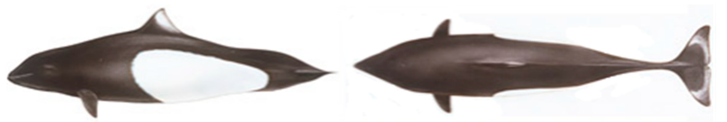
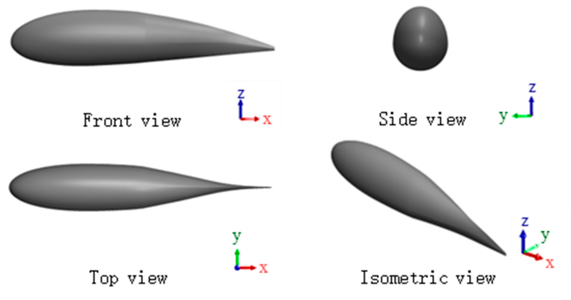
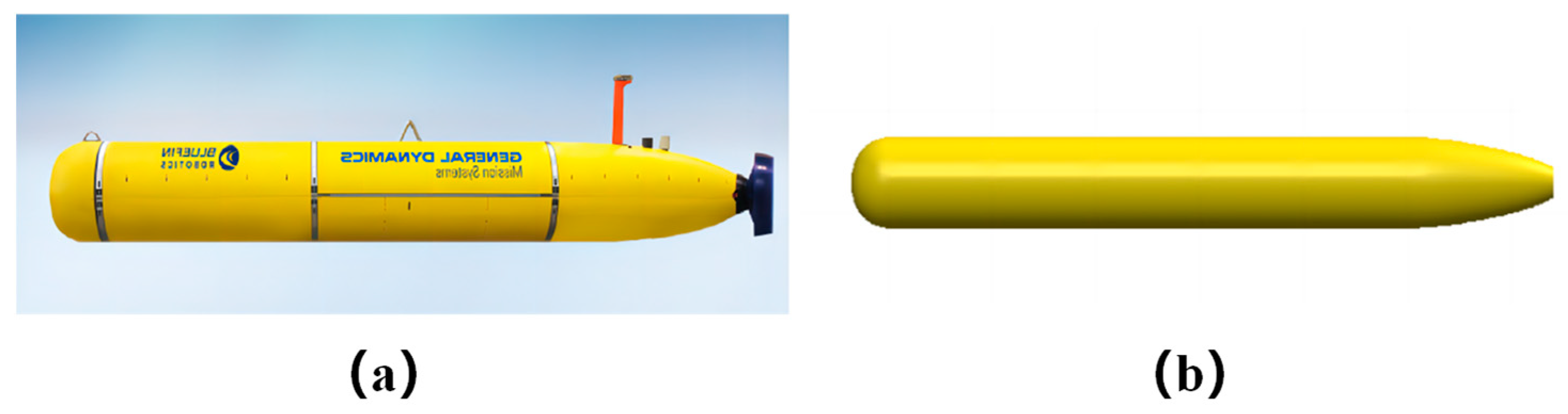
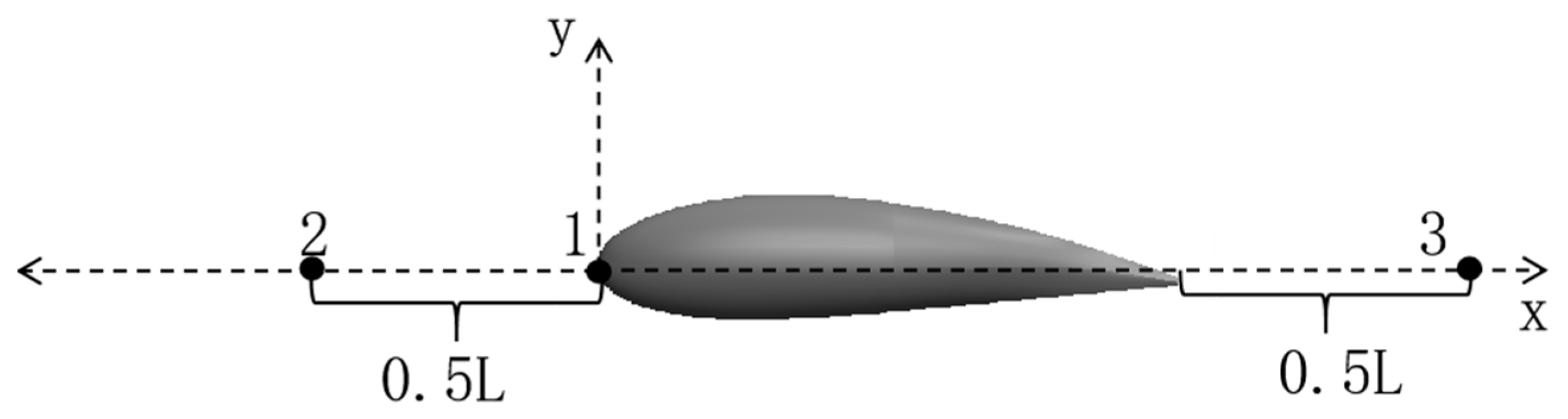
2.1. Test Models and Parameters

Modelling a bionic dolphin requires the extraction of its biomorphology. As it is difficult to obtain cetacean biological samples, a related study used an image of the beakless porpoise (Phocoenoides dalli) [15] to fit the outer contour from front and top views. Figure 1 shows images of the beakless porpoise as a contour fitting curve [16]. The effect of dorsal and caudal fins on the biomorphology was ignored in the study and the contours were smoothed.

The length of the bionic dolphin at rest was standardised to 1, measured from the tip of the dolphin’s snout to the very end of its tail vertebrae, with the tip of the snout taken as the origin of coordinates [17]. The edge contour was extracted from Figure 1 using the Canny algorithm [18]. In least-squares fitting, the goodness-of-fit (R²) for the fitted equations of the outer contour exceeded 0.98. The set of equations fitted to the contour from the front view and the set of equations fitted to the contour from the top view [1], $O_1\left(x\right)$ and $O_2\left(x\right)$, are, respectively, as follows:

$$O_1\left(x\right)=\left\{\begin{array}{c}-0.2231x^{0.5}+0.143x-0.206x^2+0.4069x^3-0.1249x^4\\ -0.0126x^{0.5}+0.7254x-1.233x^2+0.7743x^3-0.2585x^4\end{array}\right.,0\le \mathrm{x}\le 1,$$

(1)

$$O_2\left(x\right)=\left\{\begin{array}{c}0.1746x^{0.5}+0.03044x+0.2206x^2-1.083x^3+0.665x^4\\ -0.1746x^{0.5}-0.03044x-0.2206x^2+1.083x^3-0.665x^4\end{array},0\le \mathrm{x}\le 1.\right.$$

(2)

Regression analyses of O1(x) and O2(x) were performed with the National Advisory Committee for Aeronautics (NACA) wing equations.

Table 1. Residual sum of squares between the outline equations and NACA airfoil equation.

NACA Airfoil Model	Residual Sum of Squares 1 (SSE1)	Residual Sum of Squares 2 (SSE2)
2415	0.035 074 329	0.041 801 820
2418	0.022 146 282	0.028 718 003
2421	0.016 872 901	0.023 161 129
0015	0.005 232 818	/
0018	0.002 486 536	/
0021	0.007 267 699	/

presents the residual sum of squares of the profile equation and the NACA wing type equation. The NACA2421 and NACA0018 wing type equations were finally chosen as the contour equations for the front and top views of the dolphin at rest [19]. That is, for the dolphin front view, the contour equation is the asymmetric four-digit NACA2421 airfoil with the parameters c = 1, m = 0.02, p = 0.4 and t = 21. For the dolphin top view, the contour equation is the symmetric four-digit NACA0018 airfoil with the parameters c = 1 and t = 0.18. Here, c is the airfoil chord length, m is the airfoil maximum bending, p is the location of the maximum bend of the airfoil, and t is the maximum thickness of the airfoil [20].

The beakless porpoise is a medium-sized porpoise species having a typical body length of approximately 2 m [21]. Figure 2 shows the dolphin model built using the three-dimensional (3D) software Solidworks 2016 and the above equations, with a model length L of 2 m and a wet surface area of 1.696 m³.

Figure 3a shows an autonomous unmanned underwater vehicle developed by Bluefin Robotics, Inc. for a major military application, namely the Bluefin-21 [22]. The Bluefin-21 has a length of 4.93 m and a diameter of 0.53 m. However, as the design details of the shape of Bluefin-21 are not publicly available, this study modelled Bluefin-21 from high-resolution images using the CAD software Solidworks 3D 2016, as shown in Figure 3b. In this study, we mainly compared the drag characteristics of the dolphin and Bluefin-21 models, and we thus ignored the effects of other structures of Bluefin-21 on the model. The Bluefin-21 model was set to have the same length L as the dolphin model (i.e., 2 m), and a diameter of 0.215 m and a wet surface area of 1.469 m³ [23].

2.2. CFD Theory and Parameter Settings

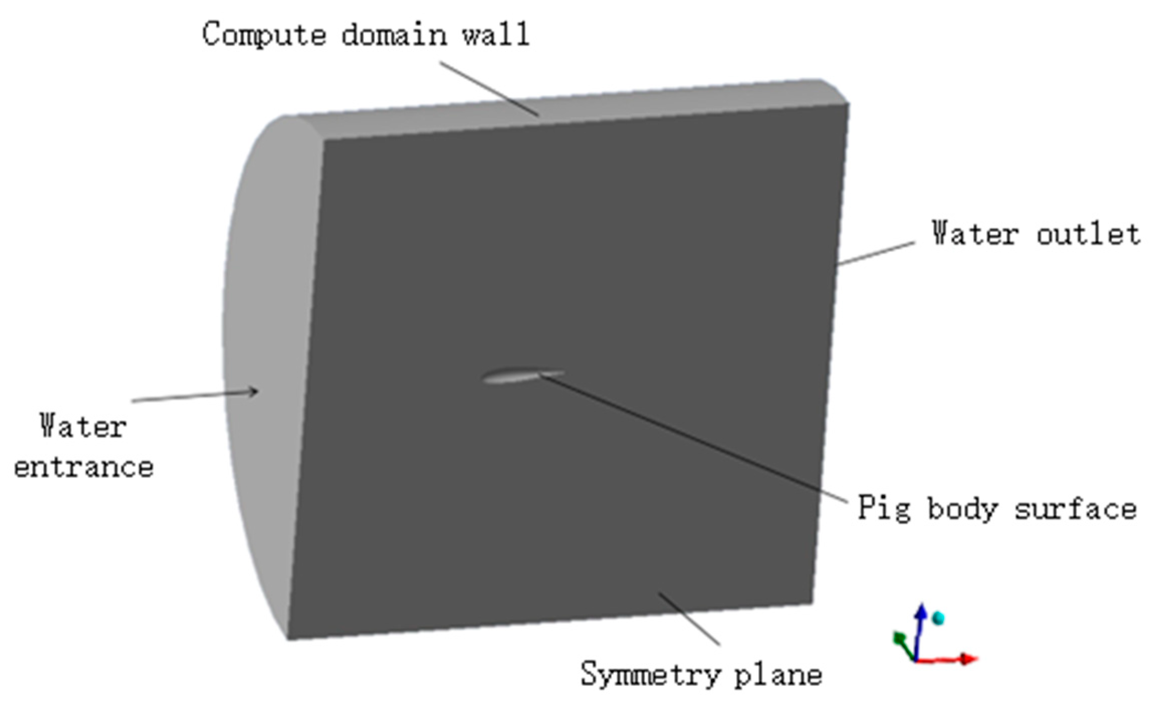
2.2.1. Computational Domain and Boundary Conditions

The CFD software Ansys Fluent 2022 was used to establish the model semi-cylindrical external flow field. The diameter is set at 6 L to reduce the adverse effect of the fluid edge on the numerical simulation results [24]. The calculation domain for the dolphin body model extends a distance of 2 L from the velocity inlet and a distance of 4 L from the pressure outlet, as illustrated in Figure 4.

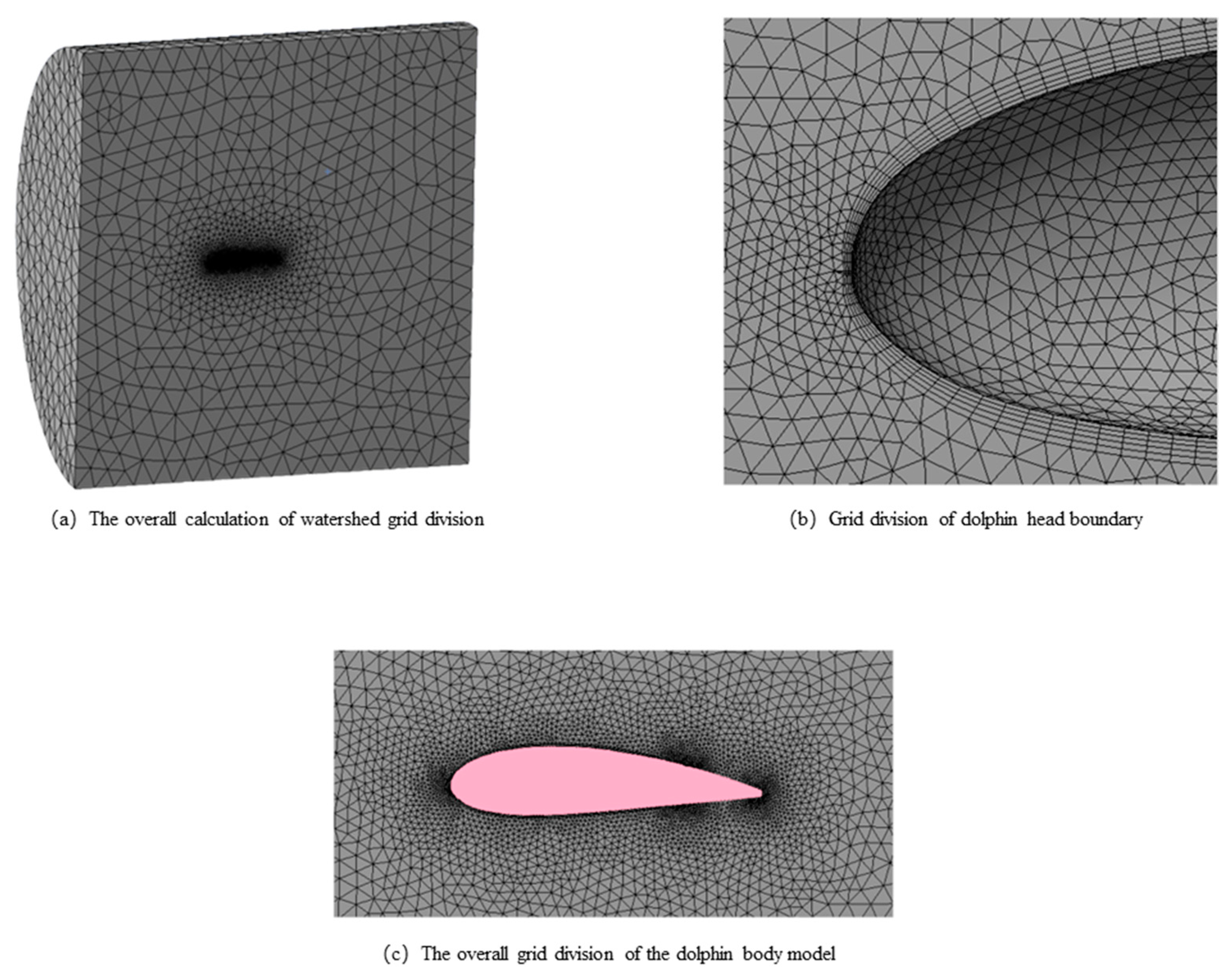
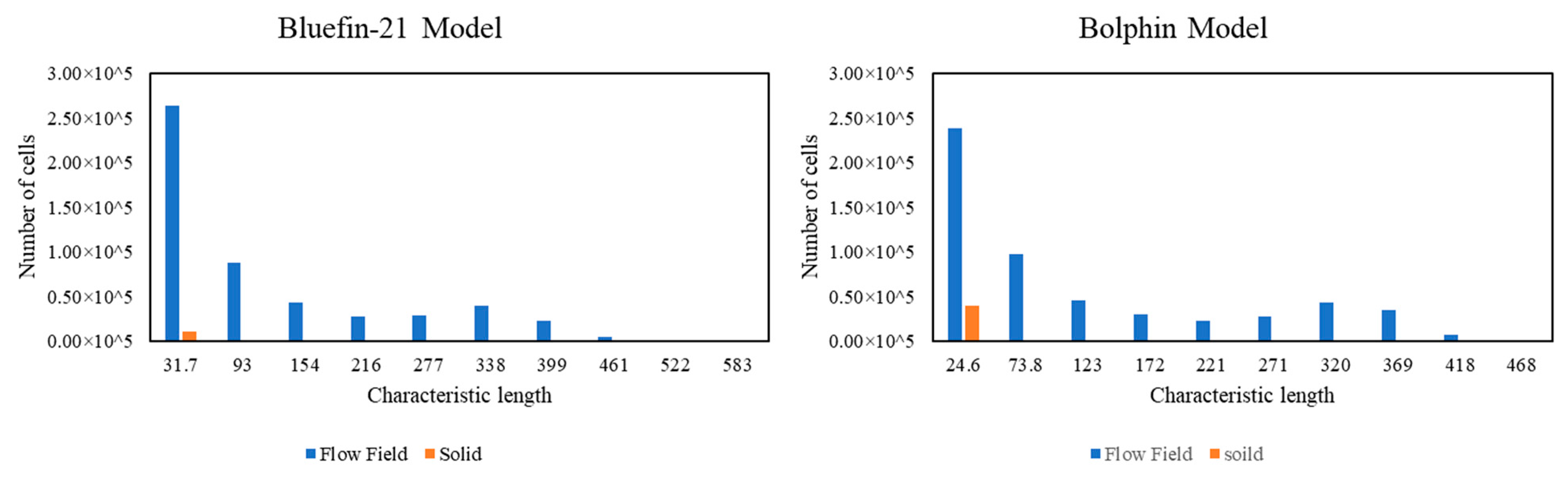
2.2.2. Mesh Parameter Settings

Although the use of a fine mesh in processing data improves the accuracy of results, it also increases the computation time of the processor. Especially when there are unnecessary details in the data, the computational requirements increase appreciably with increasing mesh fineness. Unstructured meshing of the computational domain using capture curvature and proximity methods ensures that the mesh resolution in the fluid flow region and boundary layer is sufficient for good accuracy in numerical simulation. Figure 5 shows the meshing details of the dolphin model. The maximum face size of the model surface mesh is 0.025 m, the boundary layer comprises five expansion layers, and the growth rate of the grid cells is 1.2. The average orthogonal quality of the generated mesh is 0.81. After validation of the grid closeness, the mesh comprises 714,966 cells and 138,287 nodes. To ensure consistency in the numerical simulation results of the two models, the parameter settings of the Bluefin-21 model are aligned with those of the dolphin model.

Figure 6 depicts the distribution of cell counts across various grid sizes. The mesh inspection results for the Bluefin-21 model indicate a minimum Aspect Ratio of 1.15, an Orthogonal Quality of 0.81, an average Skewness of 0.21, an average Jacobian Ratio of 1.00, and an average Wrapping Factor of 0.03. The mesh quality assessment for the dolphin model reveals a minimum Aspect Ratio of 1.15, an average Orthogonal Quality of 0.78, an average Skewness of 0.21, an average Jacobian Ratio of 1.02, and an average Wrapping Factor of 0.01.

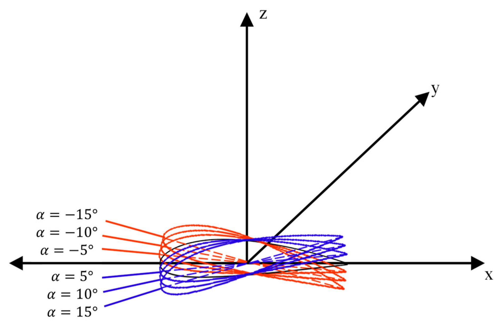
2.2.3. Setting of the Calculation Conditions

The adjustment range of the propeller pitch angle of the traditional underwater vehicle Bluefin-21 is ±15° [25]. In this paper, we mainly examine the differences in drag coefficients between the differently shaped dolphin body model and Bluefin-21 model at different pitch angles. Moreover, to ensure the accuracy and consistency of the numerical simulation results, the drag coefficients for model pitch angles of ±5°, ±10° and ±15° are selected during the calculation process. Taking the dolphin body model as an example, the pitch angle α is defined as in Figure 7.

The initial conditions and assumptions of the numerical simulation environment affect the generation of results [26]. The numerical simulation assumes three conditions: (1) the water in the basin is an incompressible fluid, and the influence of a rising wave is thus not considered; (2) the ambient temperature and density of the watershed are constant; and (3) the influence of the underwater pressure on the deformation of the model is negligible. Specific setup parameters include four flow velocity gradients set at the velocity inlets of the two models, namely flow velocities of 0.5, 1, 3 and 5 knots (kn) [27]. These velocities correspond to values of 0.26, 0.51, 1.54 and 2.57 m/s in international system units. The fluid in the computational domain is liquid water at a temperature of 20 °C.

2.2.4. Hydrodynamic Coefficient Formula

The drag characteristics of the dolphin body model and Bluefin-21 model relate to the Reynolds number Re, frictional drag coefficient C_f, differential pressure drag coefficient C_p, and total drag coefficient C_t:

$$R_e={\displaystyle \frac{\rho VL}{\mu }},$$

(3)

$$C_f={\displaystyle \frac{F_1}{\frac{1}{2}\rho V^{2}S}},$$

(4)

$$C_p={\displaystyle \frac{F_2}{\frac{1}{2}\rho V^{2}S}},$$

(5)

$$C_t={\displaystyle \frac{F_3}{\frac{1}{2}\rho V^{2}S}}.$$

(6)

here, ρ is the fluid density (kg/m³), V is the flow velocity (m/s), L is the characteristic length of the model (m), μ is the fluid viscosity coefficient (kg/m² s), F₁ is the friction resistance (N), F₂ is the differential pressure resistance (N), F₃ is the total resistance (N), and S is the wet surface area of the model (m²). The positive direction along the x-axis is specified as the positive direction of the model resistance.

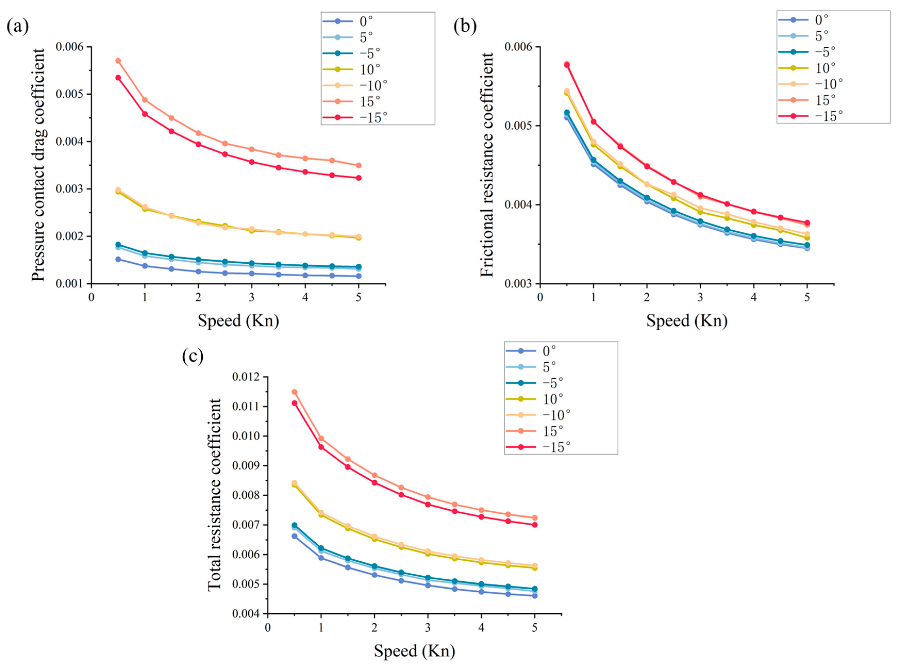
2.3. Hydrodynamic Coefficient

In this paper, the flow noise is solved for the model using the acoustic module in the CFD software Ansys Fluent 2022. On the basis of the FW-H equation and its integral solution [28], the module simulates the noise generated by equivalent sources such as monopole, dipole and quadrupole sources, and it is suitable for simulating mid- and far-field noise. In addition, it is possible to customise the position of the noise receiver to measure parameters such as the sound pressure and sound power in the flow field.

In 1952, Lighthill proposed the acoustic propagation equation, which is based on a direct derivation of the Navier–Stokes equation without introducing other assumptions or covariates [29]. This equation is important for understanding the mechanism of the generation and propagation of acoustic phenomena in fluid dynamics. Its equation is as follows:

$$\left({\displaystyle \frac{1}{c_0^2}}{\displaystyle \frac{{\partial }^2}{\partial t^2}}-{\mathsf{\nabla }}^2\right)\left[c_0^2\left(\rho -{\rho }_0\right)\right]={\displaystyle \frac{{\partial }^2{T}_{ij}}{{\partial }_{x_i}{\partial }_{x_j}}}.$$

(7)

Ffowcs Williams and Hawkings proposed the FW-H equation in 1969 [30] to describe the propagation of acoustic waves generated by an acoustic source moving in a flow field. The equation is based on Lighthill’s theory of acoustic source terms and combines the basic equations of fluid dynamics and acoustics with the equation

$${\displaystyle \frac{1}{a_0^2}}{\displaystyle \frac{{\partial }^{2}p}{\partial t^2}}-{\mathsf{\nabla }}^2{p}^{\prime }={\displaystyle \frac{\partial }{\partial t}}\left[{\rho }_0{u}_n\delta \left(f\right)\right]-{\displaystyle \frac{\partial }{{\partial }_{x_i}}}\left[P_{ij}{n}_j\delta \left(f\right)\right]+{\displaystyle \frac{{\partial }^2}{{\partial }_{x_i}{\partial }_{x_j}}}{T}_{ij},$$

(8)

where P_ij is the compressive stress tensor:

$$P_{ij}=p{\delta }_{ij}-\mu \left[{\displaystyle \frac{{\partial }_{u_i}}{{\partial }_{x_j}}}+{\displaystyle \frac{{\partial }_{u_j}}{{\partial }_{x_i}}}-{\displaystyle \frac{2}{3}}{\displaystyle \frac{{\partial }_{u_k}}{{\partial }_{x_k}}}{\delta }_{ij}\right].$$

(9)

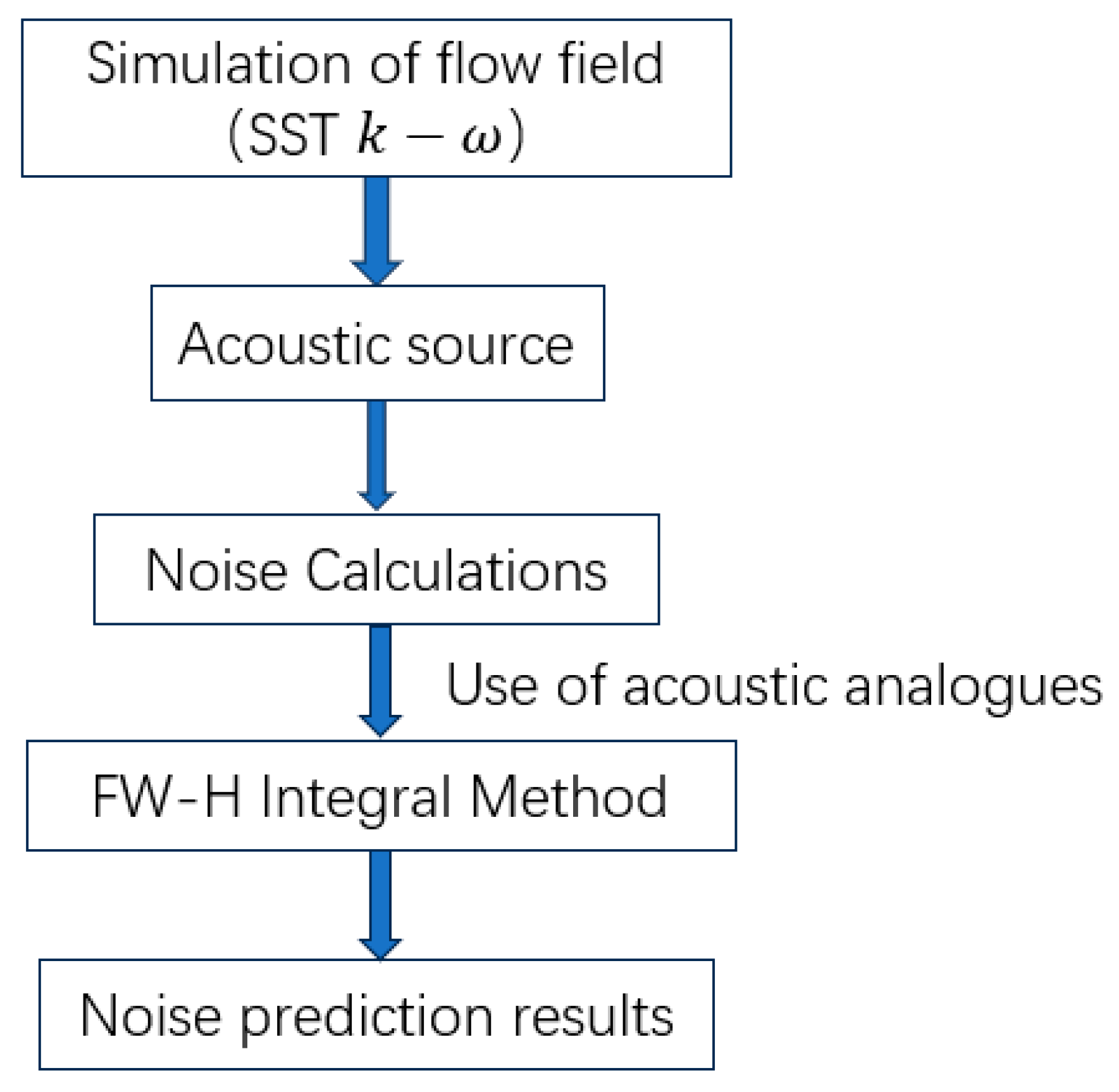
2.4. Numerical Simulation of Flow Field Noise and Calculation of the Working Conditions

In simulating the turbulent flow field in the flow noise simulation in the CFD software Ansys Fluent 2022, the shear stress transport k–ω model combined with the FW-H equation is chosen to simulate the fluid sound field, considering the high requirements of large eddy simulation on the computer hardware and the irrationality of direct numerical simulation. The simulation flow of the fluid noise calculation is shown in Figure 8. Adopting unsteady CFD simulations, we solve the acoustic sources by first calculating the turbulence information of the flow field which is calculated using the shear stress transport k–ω model so that the turbulence is fully developed. The turbulence information is then used as an input for the fluid noise calculation to solve the acoustic information in the flow field using the acoustic analogue method.

The flow noise is calculated transiently only for the model placed horizontally (at 0°). Noise receivers are set up in the acoustic field, as shown in Figure 9 for the dolphin body model. Receiver 1 is located at (0, 0, 0), receiver 2 at (−1, 0, 0), and receiver 3 at (3, 0, 0). The three receivers are positioned to clearly monitor changes in the sound pressure magnitude in the sound field, both in the front of the model head and along the axis extending forwards and backwards.

Considering only the two models placed horizontally and the situation of the maximum-speed downstream noise, the velocity at the inlet is set at 5 kn, or 2.57 m/s in international system units. At a density of water ρ = 998.2 kg/m³, the propagation speed of sound in water is 1500 m/s, and the reference acoustic pressure of the water is 1 × 10⁶ Pa. The acoustic time step satisfies the Nyquist criterion [31]:

$$f_{max}\le {\displaystyle \frac{1}{2·∆t}}$$

(10)

where f_max is the highest frequency of the spectrum to be analysed. The frequency range analysed in this chapter is 0–1000 Hz, and the acoustic time step is thus set at 0.0005 s and the maximum number of iteration steps is 20.

3. Results

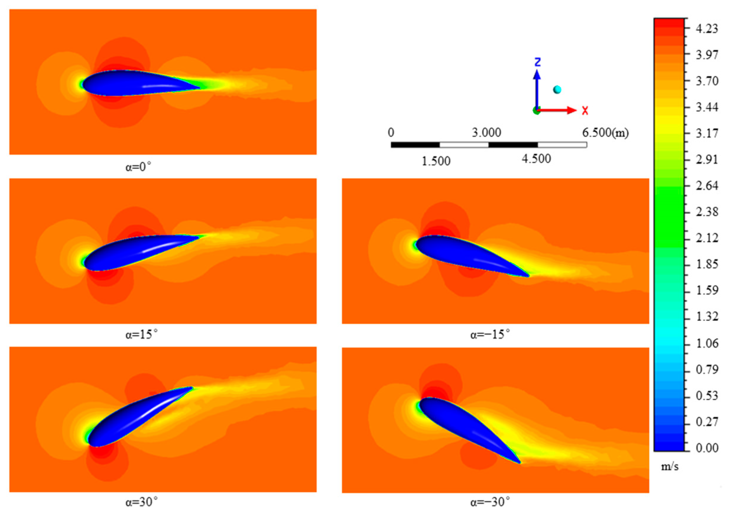
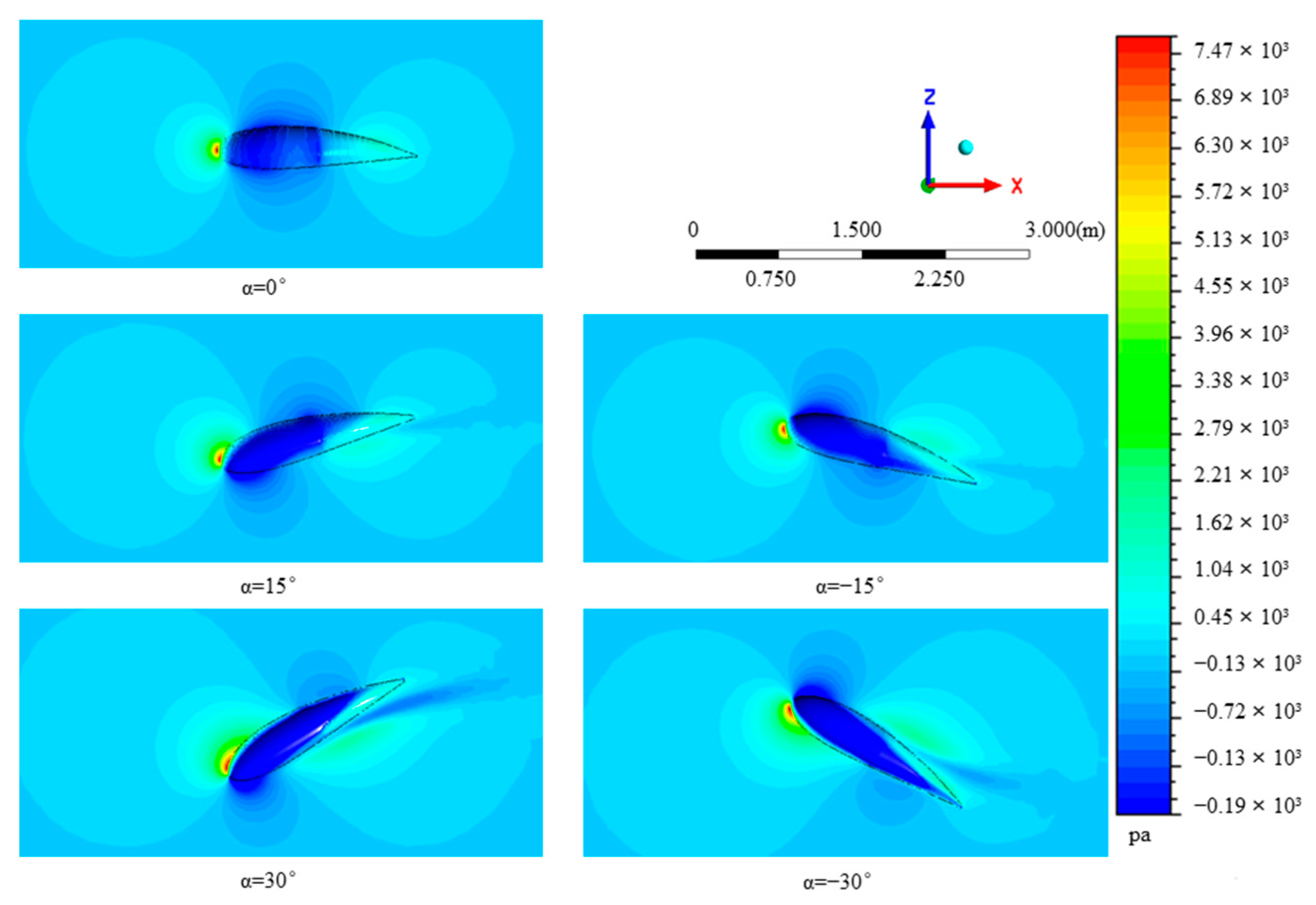
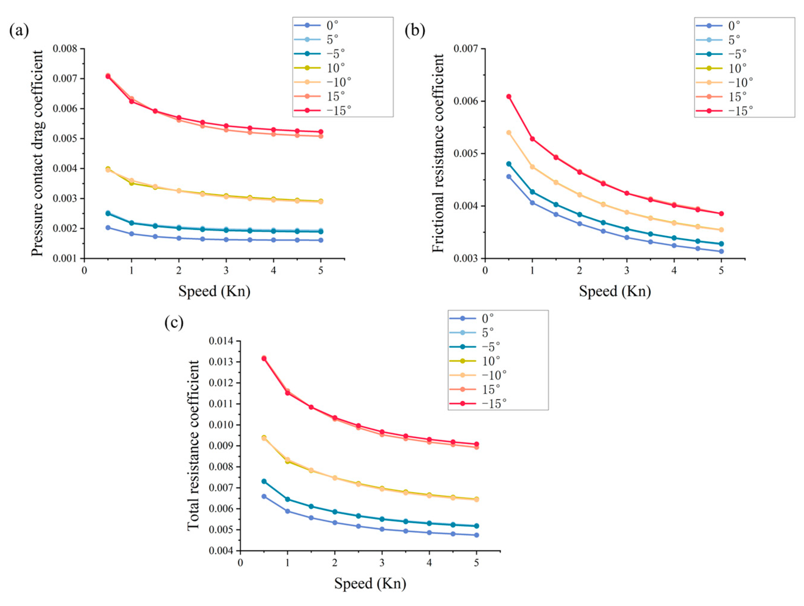
3.1. Numerical Simulation of the Drag of the Bionic Dolphin

Six pitch angles are adopted in comparing the changes in the distribution of the velocity flow field at different speeds. Figure 10 shows the numerical simulation velocity cloud of the dolphin body model at different pitch angles and an airspeed of 5 kn. In the flow field along the x-axis direction of the dolphin, there are regions near the head and tail where the velocity is lower, and the surface velocity of the dolphin first increases and then decreases. The pressure difference in the flow field outside the head of the guppy body forms a vortex that wraps around the head of the guppy body. The vortex at the head of the guppy is better wrapped around the head surface, whereas there is vortex shedding at the tail of the guppy, which becomes more obvious with an increase in the pitching angle. The difference in the flow velocity between the head and tail is larger when the guppy performs a pitching manoeuvre, and this difference helps the guppy to complete a descending or ascending manoeuvre more efficiently [32].

It is important to analyse the pressure distribution in the flow field when studying the profile drag characteristics of the dolphin body model. Figure 11 shows the pressure cloud of the dolphin body model at a speed of 5 kn. When the dolphin swims horizontally, there are areas of concentrated pressure at both the head and tail and an obvious pressure difference between the head and tail. When the dolphin model simulates a dive at a certain pitch angle, there is an obvious high-pressure region below its head; accordingly, when the dolphin model simulates an ascent at a certain elevation angle, there is an obvious high-pressure region above its head.

The differential pressure drag coefficient of the dolphin model is 0.001, 514 or 22.88% of the total drag coefficient when it is oriented horizontally (0°) and has a speed of 0.5 kn. The differential pressure drag coefficient is 23.34%, 24.45% and 25.15% of the total drag coefficient at speeds of 1, 3 and 5 kn, respectively. The drag coefficients of the dolphin model are given in

Table 2. Drag coefficients of the dolphin model at different pitch angles.

Angle of Pitch/°	Speed/kn	Pressure Contact Drag Coefficient/Cp	Frictional Resistance Coefficient/Cf	Total Resistance Coefficient/Ct	Angle of Pitch/°	Speed/kn	Pressure Contact Drag Coefficient/Cp	Frictional Resistance Coefficient/Cf	Total Resistance Coefficient/Ct
5°	0.5	0.001 765	0.005 138	0.006 903	−5°	0.5	0.001 824	0.005 168	0.006 992
	1	0.001 585	0.004 538	0.006 123		1	0.001 646	0.004 567	0.006 213
	3	0.001 378	0.003 758	0.005 136		3	0.001 430	0.003 791	0.005 221
	5	0.001 310	0.003 456	0.004 766		5	0.001 356	0.003 489	0.004 845
10°	0.5	0.002 941	0.005 415	0.008 356	−10°	0.5	0.002 979	0.005 442	0.008 421
	1	0.002 576	0.004 760	0.007 336		1	0.002 618	0.004 797	0.007 415
	3	0.002 117	0.003 907	0.006 024		3	0.002 153	0.003 956	0.006 109
	5	0.001 966	0.003 580	0.005 546		5	0.001 994	0.003 629	0.005 623
15°	0.5	0.005 703	0.005 786	0.011 489	−15°	0.5	0.005 347	0.005 767	0.011 114
	1	0.004 876	0.005 046	0.009 922		1	0.004 579	0.005 052	0.009 631
	3	0.003 837	0.004 101	0.007 938		3	0.003 568	0.004 125	0.007 693
	5	0.003 495	0.003 744	0.007 239		5	0.003 231	0.003 772	0.007 003

, and the proportion of differential pressure drag in the total drag increases gradually with increasing pitch angle. When the pitch angle is ±15°, the differential pressure drag accounts for 48.28–49.63% of the total drag as the airspeed increases. Figure 12 shows that both the differential pressure drag coefficient and friction drag coefficient decrease with increasing speed, and the magnitude of the decrease gradually decreases.

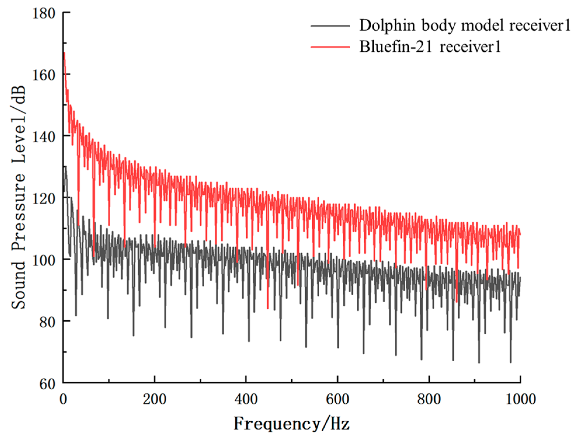
3.2. Comparison of the Morphometric Resistance between the Bionic Dolphin and Bluefin-21 Model

The Bluefin-21 model has a differential pressure drag coefficient of 0.002029, which is 30.79% of the total drag coefficient, when the model is oriented horizontally (0°) and has a speed of 0.5 kn. When the speed is 1, 3 and 5 kn, the differential pressure drag coefficient accounts for 30.96%, 32.36% and 33.92% of the total drag coefficient, respectively.

Table 3. Drag coefficients of the Bluefin-21 model at different pitch angles.

Angle of Pitch/°	Speed/kn	Pressure Contact Drag Coefficient/Cp	Frictional Resistance Coefficient/Cf	Total Resistance Coefficient/Ct	Angle of Pitch/°	Speed/kn	Pressure Contact Drag Coefficient/Cp	Frictional Resistance Coefficient/Cf	Total Resistance Coefficient/Ct
5°	0.5	0.002 531	0.004 795	0.007 326	−5°	0.5	0.002 494	0.004 804	0.007 298
	1	0.002 199	0.004 259	0.006 458		1	0.002 177	0.004 270	0.006 447
	3	0.001 978	0.003 549	0.005 527		3	0.001 935	0.003 563	0.005 498
	5	0.001 936	0.003 267	0.005 203		5	0.001 890	0.003 281	0.005 171
10°	0.5	0.003 991	0.005 401	0.009 392	−10°	0.5	0.003 948	0.005 401	0.009 349
	1	0.003 508	0.004 746	0.008 254		1	0.003 603	0.004 743	0.008 346
	3	0.003 092	0.003 879	0.006 971		3	0.003 054	0.003 878	0.006 932
	5	0.002 910	0.003 546	0.006 456		5	0.002 886	0.003 543	0.006 429
15°	0.5	0.007 104	0.006 091	0.013 195	−15°	0.5	0.007 069	0.006 085	0.013 154
	1	0.006 334	0.005 283	0.011 617		1	0.006 235	0.005 279	0.011 514
	3	0.005 286	0.004 243	0.009 529		3	0.005 426	0.004 243	0.009 669
	5	0.005 078	0.003 852	0.008 930		5	0.005 227	0.003 854	0.009 081

gives the drag coefficients of the Bluefin-21 model for different speeds and pitch angles. As the pitch angle increases, the proportion of differential pressure drag in the total drag increases. At a pitch angle of ±15°, the differential pressure drag accounts for 53.74–57.56% of the total drag as the airspeed increases.

Figure 13 presents partial drag coefficients at different pitch angles and flow speeds. The decreasing trend of the drag coefficient curves for different pitching angles flattens out as the speed increases. As the Bluefin-21 model is a rotating body, the drag coefficient curves for each part of the pitching motion basically coincide when the angles are the same.

The results of the two models are next compared and analysed. The dolphin model and Bluefin-21 model have the same length, but the wet surface area of the dolphin model is approximately 15% larger than that of the Bluefin-21 model. The difference in the total drag coefficient between the Bluefin-21 model and dolphin model is negligible when the two models are oriented horizontally at 0° and travel at speeds of 0.5–5 kn. The total drag coefficient of the Bluefin-21 model is 4.38–9.17% larger than that of the dolphin model when the two models move at a pitch angle of ±5° and a speed of 0.5–5 kn. As the dolphin model is a non-rotating body and the Bluefin-21 model is a rotating body, the differential pressure drag coefficient of the Bluefin-21 model is 43.4% larger than that of the dolphin model at a speed of 0.5 kn. The total drag coefficient of the Bluefin-21 model is 14.85–29.67% larger than that of the dolphin model when the two models travel at a pitch angle of ±15° and a speed of 0.5–5 kn. The differential pressure drag coefficient of the Bluefin-21 model is 24.57% and 29.8% larger than that of the dolphin model when the speed is 0.5 kn. As the speed increases, the differential pressure drag coefficient becomes 61.78% larger. By comparison, it is found that the differential pressure resistance of the dolphin model is less than that of the Bluefin-21 model during ascent or dive pitching manoeuvres, which helps to reduce vortex formation in the surrounding fluid.

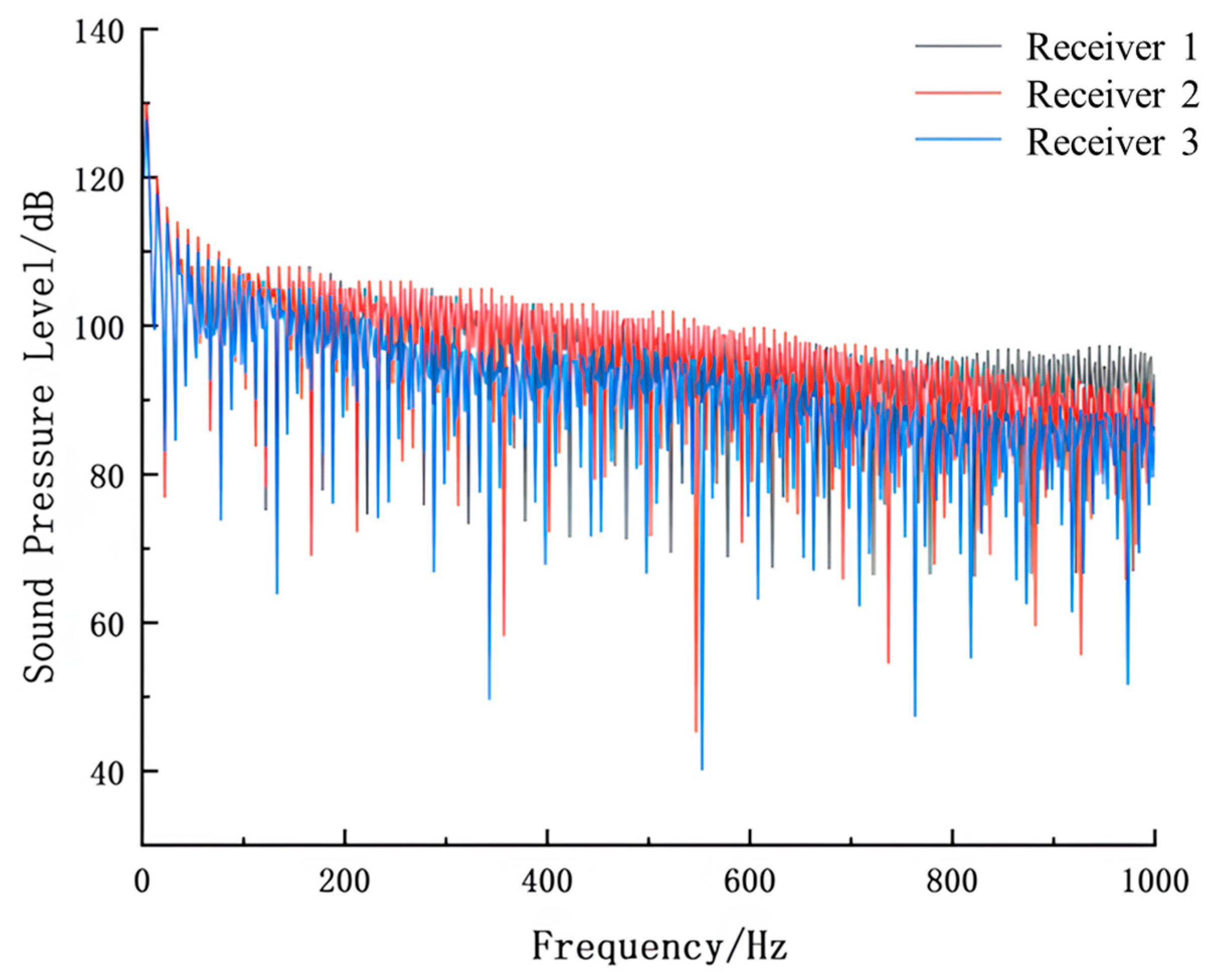
3.3. Flow Field Noise Analysis for the Bionic Dolphin

The frequency analysis of the flow noise acoustic wave involves the fast Fourier transformation of the time-domain acoustic signal obtained in the noise simulation into a spectrum analysis graph. The surface of the dolphin model is selected as the noise source, and the spectral curve of the flow noise sound pressure level (SPL) of the dolphin model oriented horizontally (0°) and travelling at 5 kn is shown in Figure 14. The figure shows that the acoustic energy is concentrated at low frequencies, and the flow noise SPL tends to decrease with an increase in frequency [33]. The frequencies corresponding to the peak values of the spectral curves of receivers 1, 2 and 3 are almost identical, with the highest values recorded as 129.88, 130.07 and 128.11 dB, respectively. In addition, the SPL spectrograms of the three streaming noise receivers are similar in shape.

The surface of the Bluefin-21 model is also taken as a noise source. Spectral curves of the SPL of the flow noise of the Bluefin-21 model placed horizontally (0°) and travelling at a speed of 5 kn are shown in Figure 15. The figure shows that the Bluefin-21 model has a higher SPL than the dolphin model at the same frequency [34]. Receivers 1, 2 and 3 streaming noise all have higher amplitudes at low frequencies [35]. As the frequency increases, the amplitude of the stream noise SPL decreases gradually. Receiver 1 has a higher SPL than receivers 2 and 3, with the peak values being 166.95, 133.95 and 132.34 dB for receivers 1, 2 and 3, respectively. A guinea pig body model has an SPL that is, respectively, 37.07 dB, 3.88 dB and 4.23 dB lower that of than the Bluefin-21 model under the same streaming noise receiver conditions [36].

The SPL of the Bluefin-21 model is appreciably lower than that of the dolphin body model, as measured by receiver 1 at the coordinate origin and shown in Figure 16. The head of the dolphin body model is rounded, which allows water to flow more smoothly to the tail, reducing turbulence and resistance. In contrast, the Bluefin-21 model with a flat head induces more turbulence and drag.

4. Discussion

4.1. Optimisation of the Morphological Construction of Bionic Underwater Submersibles

This paper compares drag for two differently shaped underwater vehicles, namely the bionic dolphin and Bluefin-21. The results show that the drag of the bionic dolphin is better than that of the traditional underwater vehicle, and that the bionic shape design is potentially valuable in the design of underwater vehicles [37]. In modelling the body of the bionic dolphin, external contour equations of the beakless porpoise from the front view and top view were derived though image processing. The method has a relatively low cost and produces a degree of visualisation that informs bionic and biological research [38]. However, image acquisition is affected by factors such as image quality and background complexity and thus requires human intervention and adjustment [39]. In further improving the accuracy and bionicity of contour extraction, machine learning and deep learning techniques can be used to filter a large number of high-quality images before contour extraction and fitting [40].

4.2. Investigation of the Drag Reduction Mechanism of Bionic Underwater Submersibles

In the study of bionic dolphins, we found that their low drag coefficients are closely related to their form factor structure [41]. However, in addition to the shape structure, the role of the skin structure in the flow field should be considered. The skin of a dolphin has special elasticity, which has an important effect on the drag coefficient when the dolphin swims in water [42]. It is thus necessary to include the elasticity coefficient of the silicone skin of a bionic dolphin in structural analysis as part of our future design work to gain a more comprehensive understanding of the drag reduction mechanism of the bionic dolphin [43]. Fluid–solid coupling analysis is an analytical method that combines fluid dynamics and solid mechanics to more accurately simulate the motion and forces of an object in a fluid [44]. In the study of the bionic dolphin, an analysis based on fluid–solid coupling can better consider the effect of skin elasticity on the drag coefficient, leading to results that better approximate real-world conditions [45].

4.3. Mechanisms for Optimising Noise in the Flow Field of Bionic Underwater Submersibles

The results of the flow noise simulation show that the receiver SPLs of the guinea pig model are lower than those of the Bluefin-21 model at different locations [46]. Among the different locations, the difference in the SPL of receiver 1 between the heads of the two models is largest because of the different shapes of the heads of the dolphin model and Bluefin-21 model [47]. Zhang Lei et al. [48] conducted noise simulations of underwater vehicles with different heads and found that the model with a smaller head radius and longer length exhibited better flow noise performance under the same conditions. Qinglong Zhang [35] carried out flow field and noise analysis on an underwater vehicle to calculate the noise radiation under three operating conditions and found that the underwater vehicle flow noise sound intensity was greatest when the shape of the front section was pointed. Jiang Yichen et al. [8] conducted CFD analysis to calculate the noise of submarines having different shapes and found that the submarine with a medium full head and a protruding transom had low drag and flow noise. These studies emphasise the importance of the head shape of an underwater vehicle to the flow noise performance [49].

5. Conclusions and Future Work

The results of this study reveal that the bionic dolphin model has advantages in terms of the differential pressure drag coefficient and total drag coefficient over the traditional underwater vehicle Bluefin-21 model under different combinations of the pitch angle and flow velocity. In addition, the ratio of the differential pressure drag to the total drag of the dolphin-body model remains at approximately 20–25% as the speed increases, whereas both the differential pressure drag and friction drag decrease with increasing speed as the pitch angle and speed increase. The dolphin-body model also demonstrates better noise performance than the Bluefin-21 model at the same speed. These findings not only provide an important theoretical basis for the drag reduction mechanism of bionic fish (or dolphins) but also provide an important reference for the design and optimisation of bionic fish.

In our study, the resistance comparison between traditional underwater vehicles and bionic dolphins under the same pitching attitude was crucial [50]. It was found that a dolphin image could be extracted through image processing, fitted with an NACA wing equation, and modelled [51]. This verifies that image processing and computational fluid dynamics numerical methods can effectively simulate the bionic dolphin [52]. However, solid model tests are necessary to further verify the accuracy of numerical simulation results [53].

Through fluid–solid coupling analysis, we clarified the specific influence of the elasticity coefficient of the silicone skin on the drag coefficient of the bionic dolphin while swimming. This insight aids in optimising the bionic dolphin design for lower drag coefficients, thereby improving swimming efficiency [54]. Additionally, fluid–solid coupling analysis helps understand the impact of the silicone skin’s elasticity on the dolphin’s stability, handling, and overall performance [55], providing a theoretical basis for practical performance optimisation [56].

The head shape of the bionic dolphin significantly affects the sound pressure level (SPL) and directly influences the drag and overall performance of the vehicle. Therefore, in designing an underwater vehicle, it is essential to consider the head shape’s effect on flow noise to optimise performance [57].

Experimental validation is the next indispensable step. Through physical tests such as flume experiments, we can verify the accuracy of the numerical simulations and gain a more comprehensive understanding of the dynamic behaviour of the bionic dolphin in an actual fluid environment. In addition, future research should consider that dynamic changes during swimming, such as those relating to the swing, pitch and yaw of the fish body, affect the overall performance of the bionic fish. Meanwhile, an in-depth study of the properties of drag components such as vortex drag and inertial drag, and their effects on the swimming performance of bionic fish, will help us to understand and optimise the drag reduction mechanism in a more comprehensive way. In terms of acoustic performance, the introduction of more advanced acoustic simulation techniques and material models will enable us to more accurately assess and optimise the acoustic properties of bionic fish. Through such comprehensive studies, we expect to further improve the design performance of bionic fish and provide stronger theoretical support and practical guidance for their performance in real applications.

References

1. Kong, X.; Huang, X.; Liu, F.; Li, B.; Wang, J.; Liu, B.; Chen, X. Design and implementation of a device based on the integration of bionic finless porpoise fish. Fish. Mod. 2021, 48, 18–25. [Google Scholar]
2. Zhang, X.; Yang, K.; Sun, Y.; Cui, H.; Jiang, J. Mechanism design of a bionic fish deep-sea exploration robot. Mechanical 2022, 49, 68–73. [Google Scholar]
3. Zhang, Y.; Li, P.; Wei, B.; Qin, H. Resistance calculation and structural design of underwater vehicle. Appl. Sci. Technol. 2023, 50, 141–148. [Google Scholar]
4. Du, X.; Shi, X.; Shi, J. Optimal design of underwater vehicle shell shape. Mech. Des. Manuf. 2005, 08, 988–990. [Google Scholar]
5. Kou, G.; Yin, H.; Dong, G.; Zhou, Y. Research on the optimal design of submarine missile package line. Shipbuild. Technol. 2012, 2, 13–17. [Google Scholar]
6. Miao, Y.; Takarata; Liu, F.; Peng, D. Shape robustness optimization of underwater vehicle based on parameterization. J. Harbin Eng. Univ. 2018, 39, 622–628. [Google Scholar]
7. Liu, F.; Liang, X.; Miao, Y.; Tu, C.; Zhao, Y. Parametric analysis and optimization of drag of underwater vehicles. J. Unmanned Underw. Syst. 2020, 28, 526–531. [Google Scholar]
8. Jiang, Y.; Zhao, Y.; Xiong, J.; Yang, Y.; Zhang, G. Comprehensive effects of hull shape on drag and flow noise of underwater vehicles. J. Harbin Eng. Univ. 2022, 43, 76–82+138. [Google Scholar]
9. Panda, J.P.; Mitra, A.; Warrior, H.V. A review on the hydrodynamic characteristics of autonomous underwater vehicles. Proc. Inst. Mech. Eng. Part M J. Eng. Marit. Environ. 2020, 235, 15–29. [Google Scholar] [CrossRef]
10. Vardhan, H.; Sztipanovits, J. Search for Universal Minimum Drag Resistance Underwater Vehicle Hull Using CFD. In Computational and Experimental Simulations in Engineering; Springer: Cham, Switzerland, 2024; pp. 1297–1303. [Google Scholar]
11. Lingshuai, M.; Lin, Y.; Xu, H.; Gu, H. Effects of front shapes of mini revolving AUV on sailing resistance characteristics. In Proceedings of the 2015 IEEE International Conference on Information and Automation, Lijiang, China, 8–10 August 2015; pp. 1795–1799. [Google Scholar]
12. Khalin, A.; Kizilova, N. Performance comparison of different aerodynamic shapes for autonomous underwater vehicles. Arch. Mech. Eng. 2019, 66, 171–189. [Google Scholar] [CrossRef]
13. Chen, Y.; Zhou, L. Bionics and the development of weapons and equipment. Mod. Weapons 1989, 6, 9–12. [Google Scholar]
14. Yu, J.; Wu, Z. Natural Inspiration Technology Inspiration, Bionic Improves Maneuverability: Interpretation of “Design and Control Technology of High Mobility Bionic Robot Fish”. China Mech. Eng. 2019, 4, 498–503. [Google Scholar]
15. Huang, S.; Hu, Y.; Wang, Y. Research on aerodynamic performance of a novel dolphin head-shaped bionic airfoil. Energy 2021, 214, 118179. [Google Scholar] [CrossRef]
16. Zhou, K.; Liu, J.; Chen, W. Numerical Study on Hydrodynamic Performance of Bionic Caudal Fin. Appl. Sci. 2016, 6, 15. [Google Scholar] [CrossRef]
17. Liu, H. Research on Autonomous Swimming of Tuna-like Underwater Robot. Ph.D. Thesis, Harbin Engineering University, Harbin, China, 2017. [Google Scholar]
18. Liu, X.; Qiu, J.; Wu, X. License Plate Localization Algorithm Based on Deep Learning and Color Edge Features. Comput. Eng. Des. 2020, 41, 2942–2948. [Google Scholar] [CrossRef]
19. Zhang, S. Discussion on the goodness-of-fit index of curve regression. Chin. J. Health Stat. 2002, 1, 9–11. [Google Scholar]
20. Liu, F.; Zou, J.; Zheng, Y. The influence of physical parameters of the synthetic jet on the control of airfoil flow separation. J. ZheJiang Univ. 2013, 47, 146–153. [Google Scholar]
21. Jefferson, T.A. D—Dall’s Porpoise Phocoenoides dalli. In Encyclopedia of Marine Mammals, 2nd ed.; Perrin, W.F., Würsig, B., Thewissen, J.G.M., Eds.; Academic Press: London, UK, 2009; pp. 296–298. [Google Scholar]
22. LeHardy, P.K.; Moore, C. Deep ocean search for Malaysia airlines flight 370. In Proceedings of the 2014 Oceans—St. John’s, St. John’s, NL, Canada, 14–19 September 2014; pp. 1–4. [Google Scholar]
23. Deep-Sea Tracker—“Bluefin” [EB/OL]. Available online: https://weibo.com/ttarticle/p/show?id=2309404266218138787588 (accessed on 27 July 2018).
24. Liu, J. Improvement of the shear stress transport k-ω turbulence model in the compressible separated flow of slender projectiles. Sci. Technol. Eng. 2018, 18, 142–147. [Google Scholar]
25. Cao, Q. Analysis of technical characteristics of “Bluefin Tuna-21” autonomous underwater vehicle. Electro-Opt. Syst. 2014, 2, 1–6. [Google Scholar]
26. Xue, W.; Xiong, Y. Numerical simulation of the initial value problem of liquid sloshing based on shallow water wave theory. J. Dyn. Control 2015, 13, 308–313. [Google Scholar]
27. Pan, D. Research on the Detection Principle Based on the Flow Field of Underwater Moving Bodies. Master’s Thesis, Beijing Institute of Technology, Beijing, China, 2020. [Google Scholar]
28. He, J.; Wang, Y.; Liu, Q.; Qian, Z. Mechanism and suppression method of pseudosound generation of permeable convection FW-H equation. Chin. J. Aerodyn. 2023, 41, 16–25. [Google Scholar]
29. Bose, T. Lighthill’s Theory of Aerodynamic Noise. In Aerodynamic Noise: An Introduction for Physicists and Engineers; Bose, T., Ed.; Springer: New York, NY, USA, 2013; pp. 53–60. [Google Scholar]
30. Ribeiro, A.F.P.; Khorrami, M.R.; Ferris, R.; König, B.; Ravetta, P.A. Lessons learned on the use of data surfaces for Ffowcs Williams-Hawkings calculations: Airframe noise applications. Aerosp. Sci. Technol. 2023, 135, 108202. [Google Scholar] [CrossRef]
31. Kopitz, J.; Polifke, W. CFD-based application of the Nyquist criterion to thermo-acoustic instabilities. J. Comput. Phys. 2008, 227, 6754–6778. [Google Scholar] [CrossRef]
32. Song, W.; Wang, C.; Wei, Y.; Xu, H.; Lu, J. Experimental study on drag reduction characteristics of microbubbles in pitching motion of underwater vehicles. Acta Armamentarii Sin. 2019, 40, 1902–1910. [Google Scholar]
33. Cao, K. Aerodynamic performance and noise study of variable-cross-section three-dimensional wing. Agric. Equip. Veh. Eng. 2023, 61, 114–119. [Google Scholar]
34. Yu, L.; Zhao, W.; Wan, D. A review of the research and application progress of hydrodynamic noise calculation methods at water-gas interface. Chin. J. Ship Res. 2022, 17, 85–102. [Google Scholar] [CrossRef]
35. Zhang, Q. Numerical Analysis and Study of Hydrodynamic Noise of an Underwater Vehicle. Master’s Thesis, Kunming University of Science and Technology, Kunming, China, 2022. [Google Scholar]
36. Zhang, Y. The concept and technology development of autonomous underwater vehicle technology—Taking “bluefin-21” as an example. China Terminol. 2014, 16, 131. [Google Scholar]
37. Zifan, W.; Qiang, Y.; Songlin, Y. Analysis of the Resistance Performance for Different Types of AUVs Based on CFD. Chin. Ship Res. 2014, 9, 28–37. [Google Scholar]
38. Zhang, Y.; Song, Z.; Wang, X.; Cao, W.; Au, W.W. Directional acoustic wave manipulation by a porpoise via multiphase forehead structure. Phys. Rev. Appl. 2017, 8, 064002. [Google Scholar] [CrossRef]
39. Feng, X.; Shen, Y.; Wang, D. A survey on the development of image data augmentation. Comput. Sci. Appl 2021, 11, 370–382. [Google Scholar]
40. Mziou-Sallami, M.; Khalsi, R.; Smati, I.; Mhiri, S.; Ghorbel, F. DeepGCSS: A robust and explainable contour classifier providing generalized curvature scale space features. Neural Comput. Appl. 2023, 35, 17689–17700. [Google Scholar] [CrossRef]
41. Tan, Z.; Zhang, C.; Sun, Z.; Gao, N.; Jia, Y.; Xie, G. A six-degree-of-freedom bionic machine dolphin. Ordnance Autom. 2022, 41, 25–29. [Google Scholar]
42. Ma, Z.; Chen, R.; Qu, Y.; Kong, Y.; Hu, K.; Zhou, Q.; Xu, S.; Yan, Z.; Yang, Y.; He, H. Hydrodynamic control of silicone elastomers on between porous media. J. Ind. Text. 2024, 54, 15280837241227246. [Google Scholar] [CrossRef]
43. Jurásková, A.; Olsen, S.M.; Skov, A.L. Reversible Dynamic Behavior of Condensation-Cured Silicone Elastomers Caused by a Catalyst. Macromol. Mater. Eng. 2023, 308, 2200615. [Google Scholar] [CrossRef]
44. Li, W.; Desbrun, M. Fluid-Solid Coupling in Kinetic Two-Phase Flow Simulation. ACM T. Graph. 2023, 42, 123. [Google Scholar] [CrossRef]
45. Xia, D.; Li, Z.; Lei, M.; Yan, H.; Zhou, Z. A comparative and collaborative study of the hydrodynamics of two swimming modes applicable to dolphins. Biomimetics 2023, 8, 311. [Google Scholar] [CrossRef] [PubMed]
46. Zimmerman, R.; Spain, G.L.D.; Chadwell, C.D. Decreasing the radiated acoustic and vibration noise of a mid-size AUV. IEEE J. Ocean. Eng. 2005, 30, 179–187. [Google Scholar] [CrossRef]
47. Zhang, C.; Song, Z.-C.; Zhang, Y. Sound reception pathway of the Indo-Pacific humpback dolphin. Acta Phys. Sin. 2020, 69, 202–209. [Google Scholar] [CrossRef]
48. Zhang, L.; Fan, L.; Shen, L.; Zhang, J.; Sun, J.; Wang, C. Numerical simulation of head flow noise performance of underwater vehicle. Ship Sci. Technol. 2017, 39, 14–19. [Google Scholar]
49. Liu, H. Flow-Induced Noise Characteristic Analysis of Submarine Flow Cavity Based on Large Eddy Simulation. In Proceedings of the ISOPE International Ocean and Polar Engineering Conference, Hangzhou, China, 11–16 October 2020; p. ISOPE–I-20-4197. [Google Scholar]
50. Xu, J.; Fang, W.; Fan, W.; Wang, Q.; Gu, Y. The Research of the Drag Reduction of Non-Smooth Underwater Vehicle. Int. J. Fluid Dyn. 2024, 12, 121001. [Google Scholar] [CrossRef]
51. Yu, Y. Numerical Investigation on Aerodynamic Performance of NACA0018 Airfoil Serrated Gurney Flap. Model. Simul. 2021, 10, 578–585. [Google Scholar] [CrossRef]
52. Steenwijk, B.; Druetta, P. Numerical Study of Turbulent Flows over a NACA 0012 Airfoil: Insights into Its Performance and the Addition of a Slotted Flap. Appl. Sci. 2023, 13, 7890. [Google Scholar] [CrossRef]
53. Smith, B.L. The difference between traditional experiments and CFD validation benchmark experiments. Nucl. Eng. Des. 2017, 312, 42–47. [Google Scholar] [CrossRef]
54. Yu, J.; Liu, Z.; Wu, W. Research progress on dolphin skin drag reduction and noise reduction. In Proceedings of the 15th Symposium on Underwater Noise of Ships and the 30th Anniversary of the Establishment of the Underwater Noise Group of the Academic Committee of Ship Mechanics, Zhengzhou, China, 1 August 2015; p. 8. [Google Scholar]
55. Xia, D.; Li, Z.; Lei, M.; Shi, Y.; Luo, X. Hydrodynamics of Butterfly-Mode Flapping Propulsion of Dolphin Pectoral Fins with Elliptical Trajectories. Biomimetics 2023, 8, 522. [Google Scholar] [CrossRef] [PubMed]
56. Chen, L.; Liu, S.-g.; Zhao, D.; Dong, L.-q.; Li, K.; Tang, S.; Cui, J.; Guo, H. Research on the flow stability and noise reduction characteristics of quasi-periodic elastic support skin. Def. Technol. 2024, 33, 222–236. [Google Scholar] [CrossRef]
57. Shi, S.; Huang, X.; Rao, Z.; Su, Z.; Hua, H. Numerical analysis on flow noise and structure-borne noise of fully appended SUBOFF propelled by a pump-jet. Eng. Anal. Bound. Elem. 2022, 138, 140–158. [Google Scholar] [CrossRef]
Figure 1. Front and top views of Phocoenoides dalli.
Jmse 12 01373 g001
Figure 2. Three-dimensional dolphin model.
Jmse 12 01373 g002
Figure 3. Bluefin-21 front view and three-dimensional modelling front view. (a) Bluefin-21 physical; (b) Bluefin-21 model.
Jmse 12 01373 g003
Figure 4. Computational domain of the dolphin body model.
Jmse 12 01373 g004
Figure 5. Mesh generation.
Jmse 12 01373 g005
Figure 6. The number of cells with different grid sizes.
Jmse 12 01373 g006
Figure 7. Definition of pitch angle α.
Jmse 12 01373 g007
Figure 8. Simulation flow of the fluid noise calculation.
Jmse 12 01373 g008
Figure 9. Schematic showing the noise receiver locations.
Jmse 12 01373 g009
Figure 10. Velocity cloud diagrams for different pitch angles of the dolphin body model.
Jmse 12 01373 g010
Figure 11. Pressure cloud diagrams for different pitch angles of the dolphin body model.
Jmse 12 01373 g011
Figure 12. Resistance coefficients of the dolphin body model. (a) The pressure drag coefficient of the dolphin body model; (b) The friction drag coefficient of the dolphin body model; (c) The total drag coefficient of the dolphin body model.
Jmse 12 01373 g012
Figure 13. Resistance coefficients of the Blufin-21 model. (a) The pressure drag coefficient of the Bluefin-21 model; (b) The friction drag coefficient of the Bluefin-21 model; (c) The total drag coefficient of the Bluefin-21 model.
Jmse 12 01373 g013
Figure 14. Spectral curves of the sound pressure levels for the flow noise of the dolphin body model.
Jmse 12 01373 g014
Figure 15. Spectral curves of the sound pressure level for the flow noise of the Bluefin-21 model.
Jmse 12 01373 g015
Figure 16. Spectral curves of the stream noise sound pressure level for receiver 1.
Jmse 12 01373 g016