
Research on the Flow-Induced Vibration of Cylindrical Structures Using Lagrangian-Based Dynamic Mode Decomposition


Abstract
:1. Introduction
2. L-DMD Method
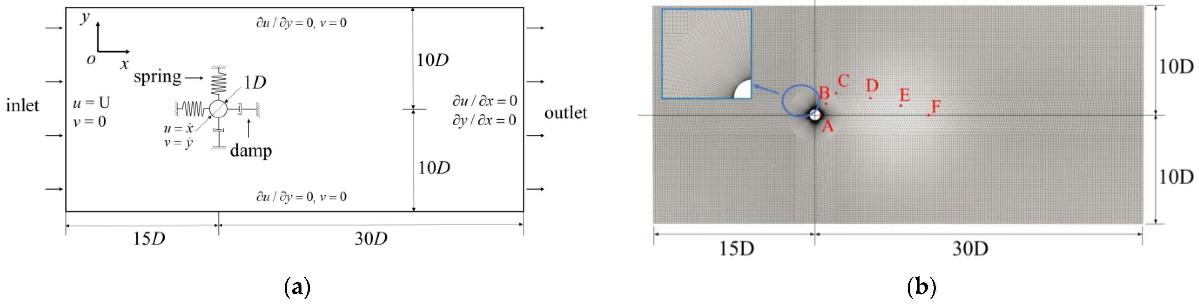
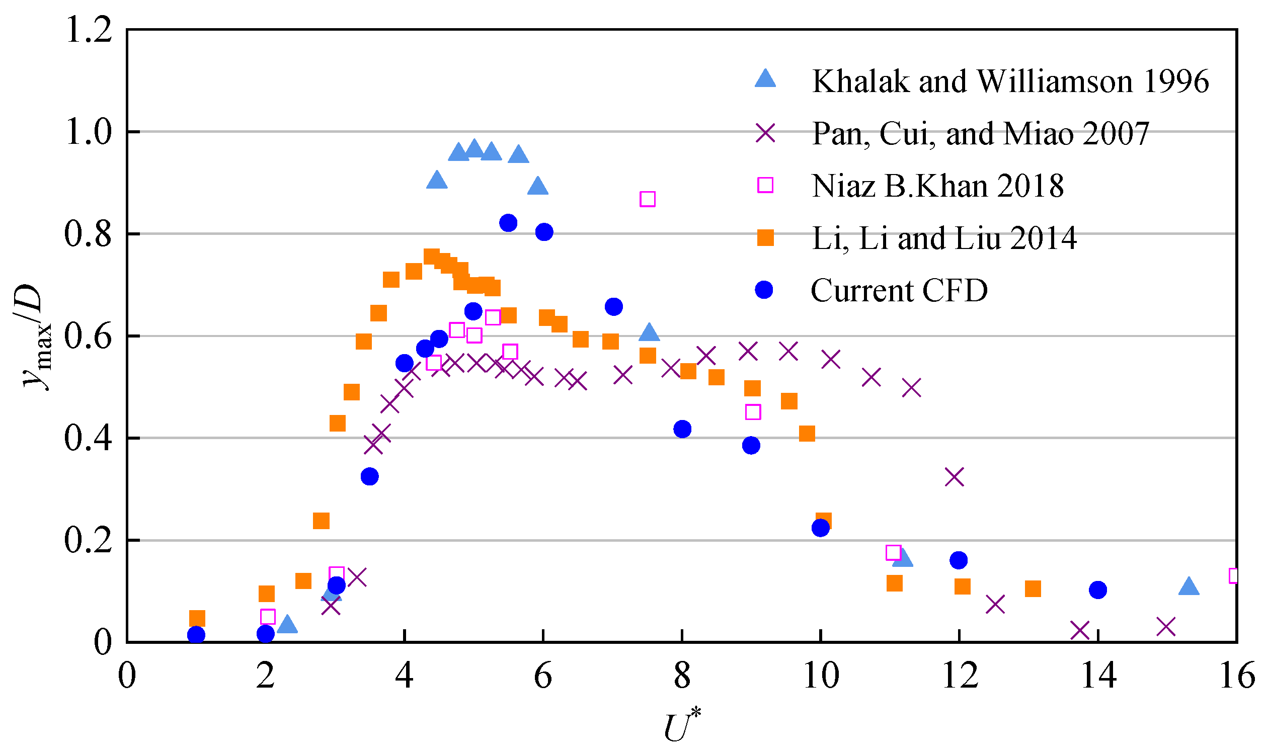
3. Numerical Models
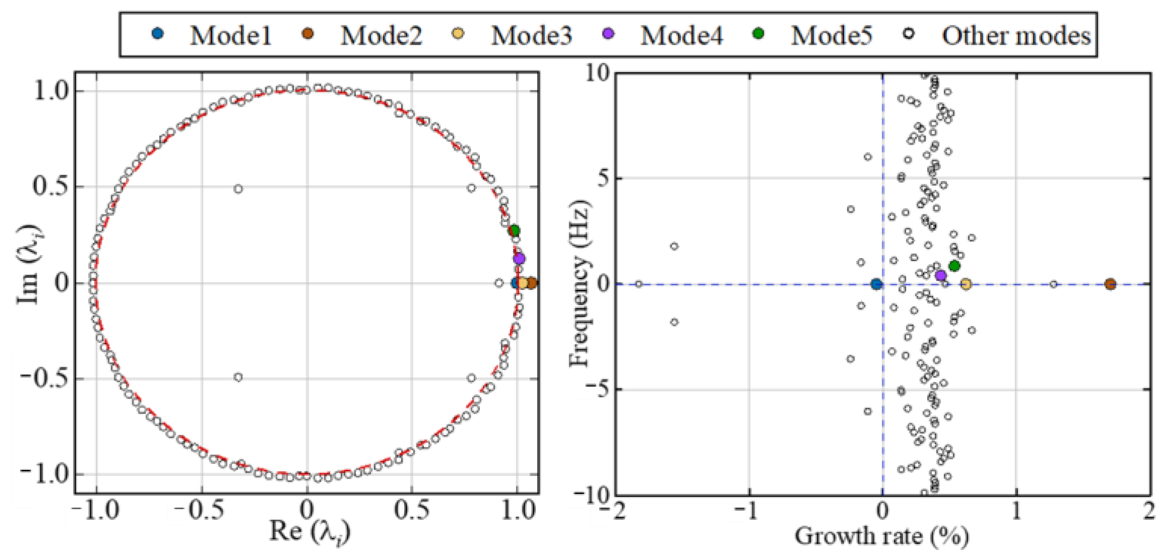
4. Analysis Based on L-DMD
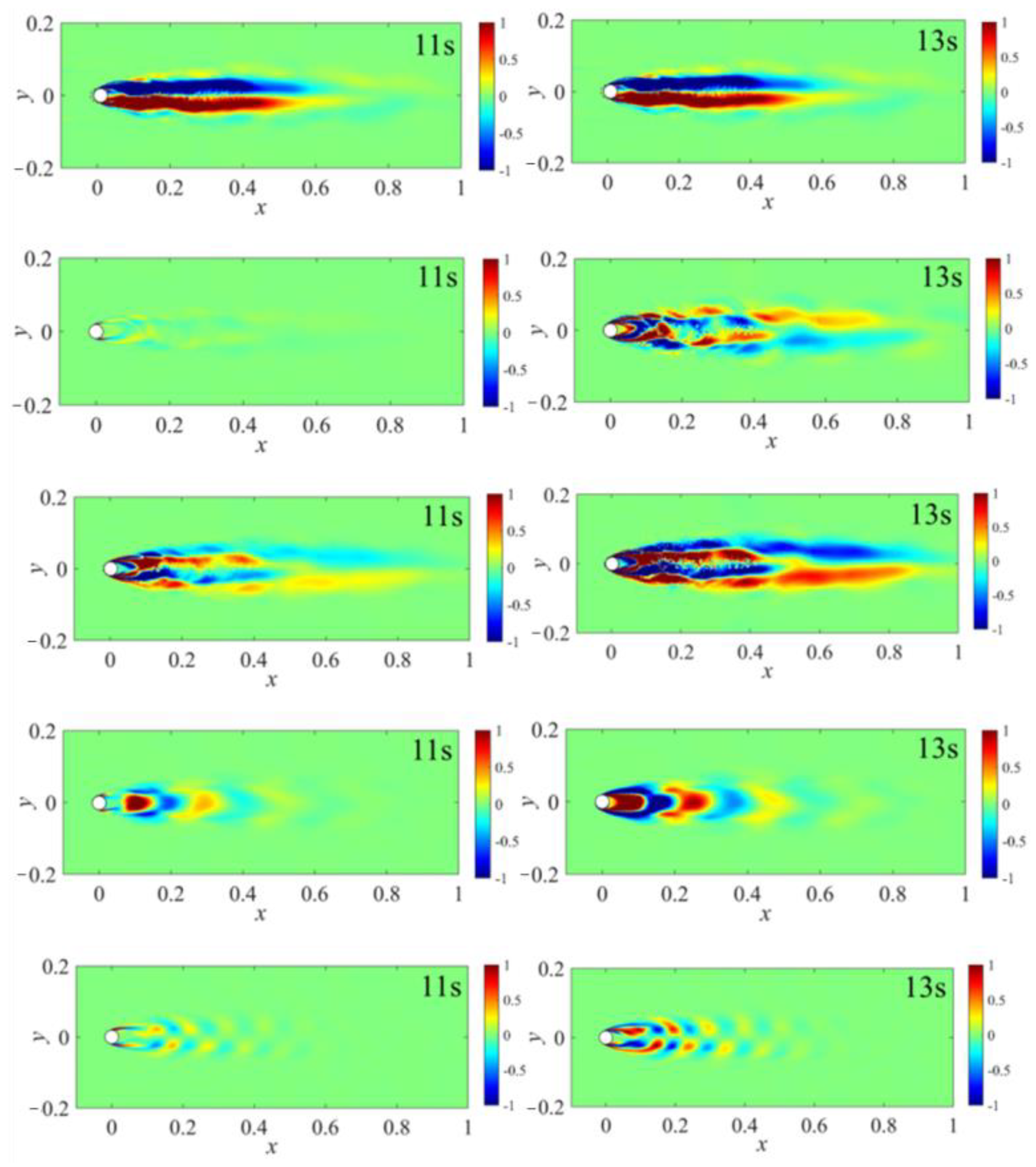
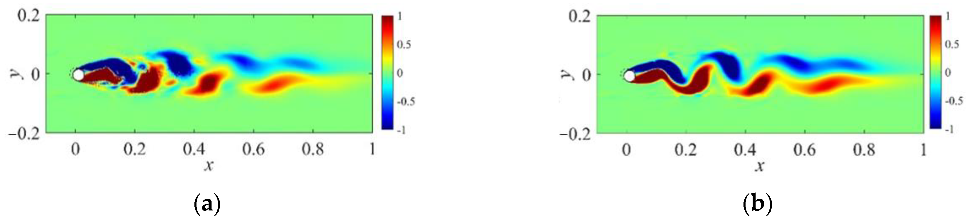
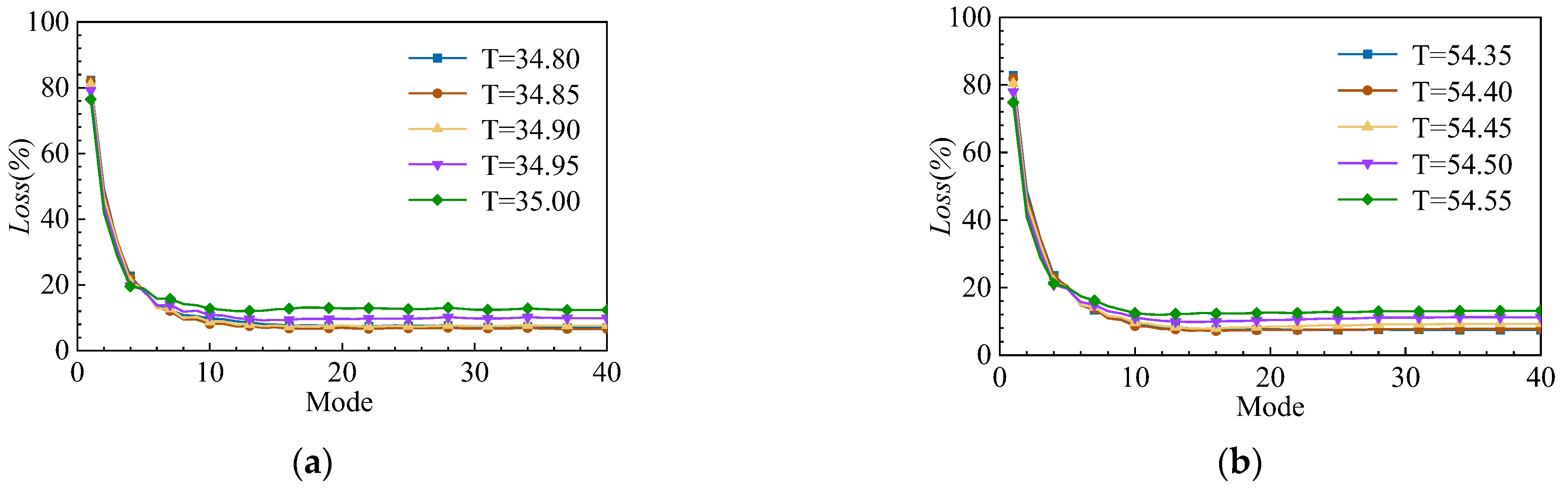
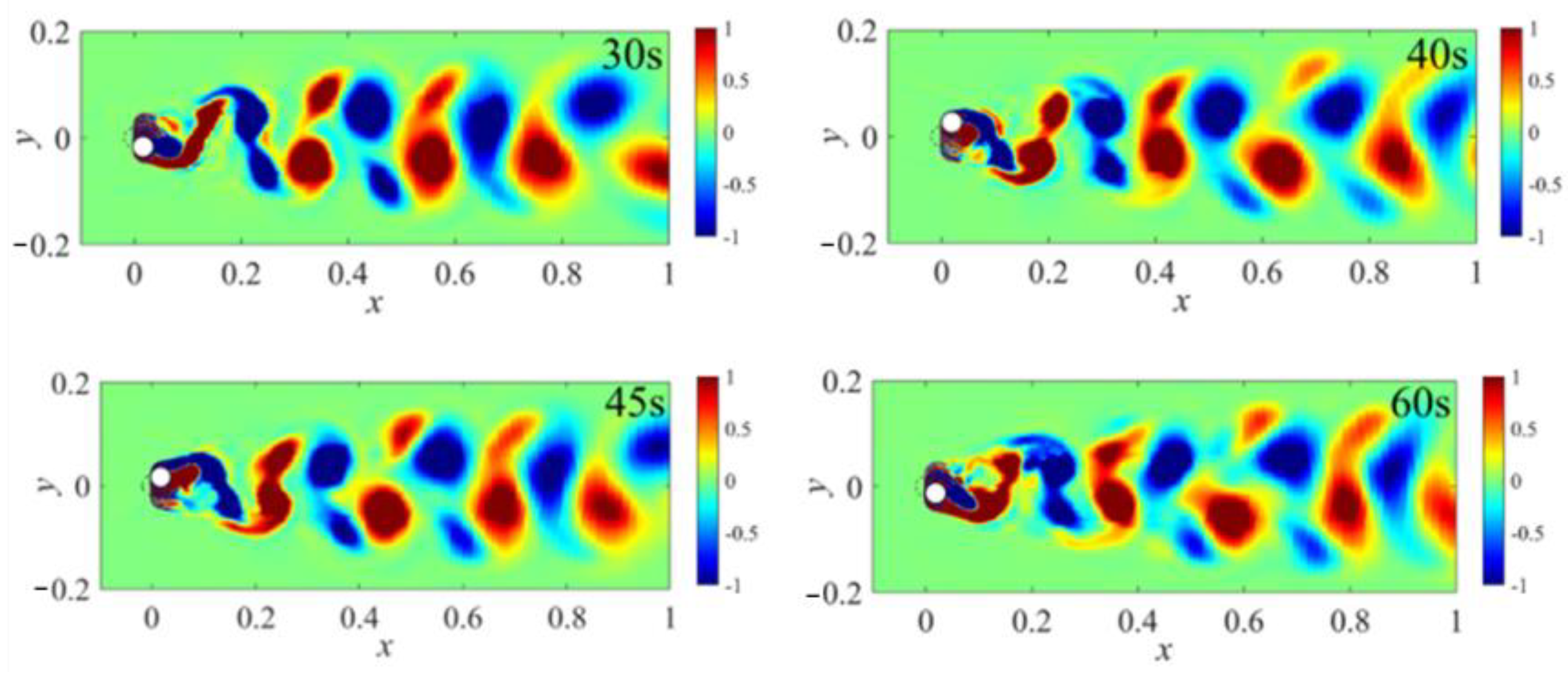
4.1. Development Stage
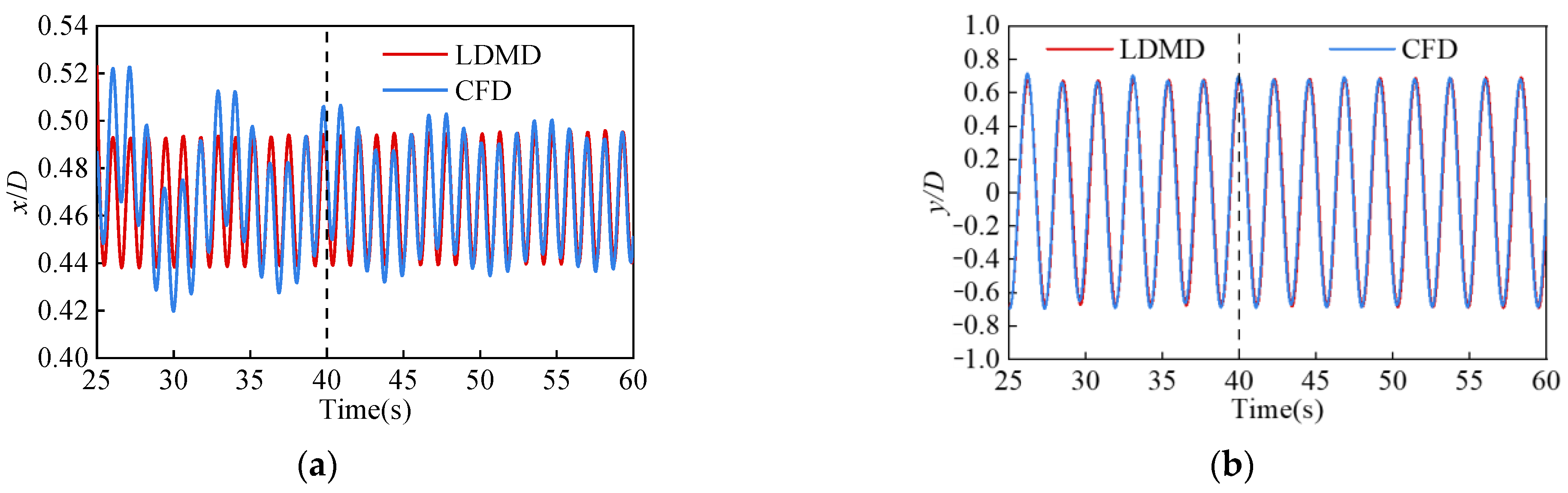
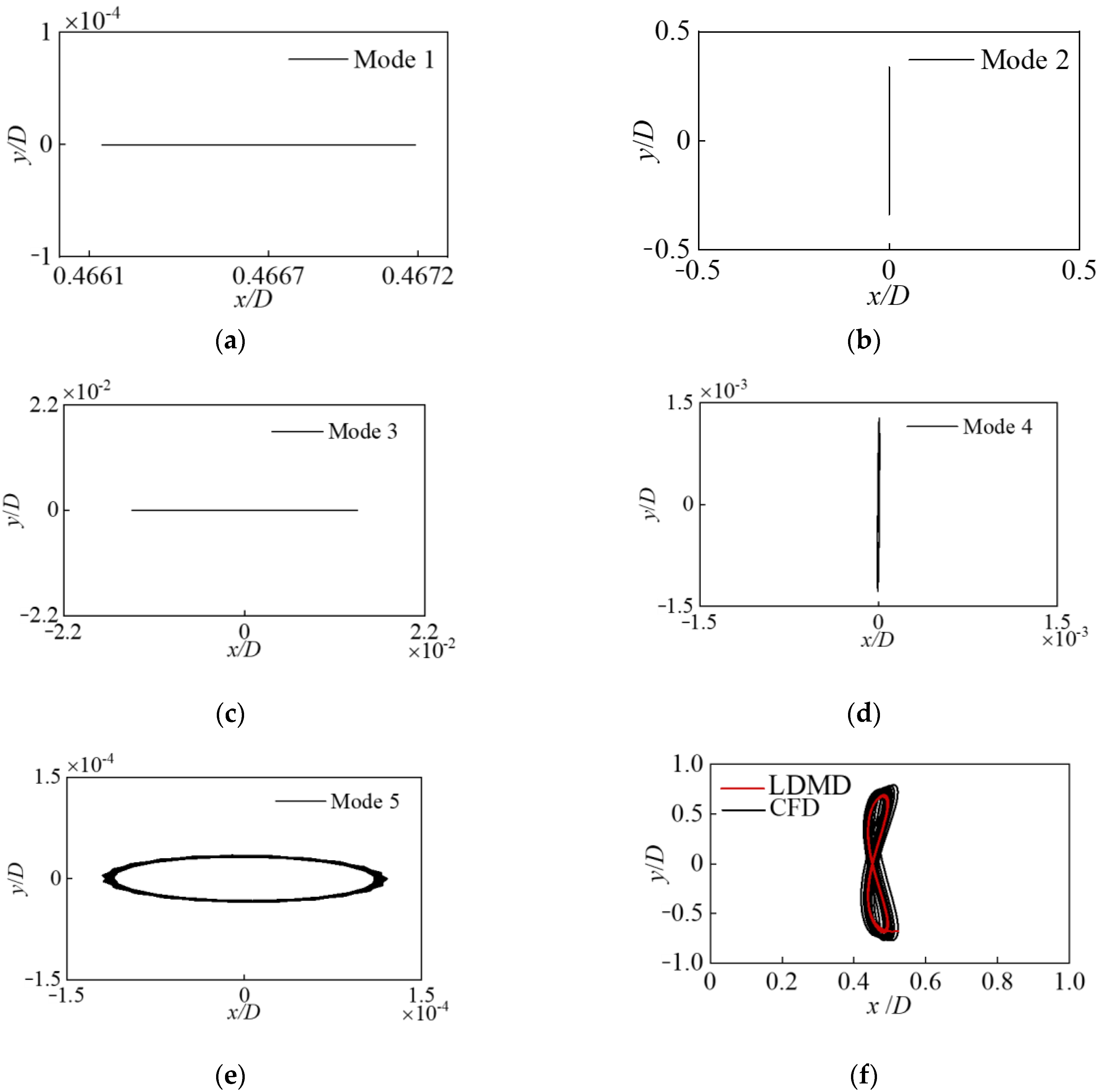
4.2. Stable Stage
5. Conclusions
Author Contributions
Funding
Institutional Review Board Statement
Informed Consent Statement
Data Availability Statement
Conflicts of Interest
Nomenclature
| m | Grid node number |
| n | Total number of snapshots |
| i | ith snapshot |
| k | kth mode |
| xi | ith snapshot flow field data vector |
| Pi | Displacement vector of the ith snapshot node |
| X | All snapshot data matrices |
| X1 | The 1 to (n − 1) snapshot data matrix |
| X2 | The 2 to n snapshot data matrix |
| U | Matrix containing all modes |
| V | Matrix containing temporal information of spatial matrix U |
| A | System matrix of high-dimensional flow field |
| Reduced-order matrix of A | |
| kth modal eigenvalue | |
| W | Eigenvector matrix |
| Modal matrix | |
| kth modal eigenvector | |
| b | Modal amplitude matrix |
| bk | kth modal amplitude |
| P | Grid node displacement matrix |
| D | Cylinder diameter |
| m*ζ | Mass damping ratio |
| U* | Reduced velocity |
| x/D | Non-dimensional in-line displacement |
| y/D | Non-dimensional crossflow displacement |
| Frobenius normalization |
References
- Wang, K.; Tang, W.; Xue, H. Time domain approach for coupled cross-flow and in-line VIV induced fatigue damage of steel catenary riser at touchdown zone. Mar. Struct. 2015, 41, 267–287. [Google Scholar] [CrossRef]
- Liu, Z.; Shen, J.; Li, S.; Chen, Z.; Ou, Q.; Xin, D. Experimental study on high-mode vortex-induced vibration of stay cable and its aerodynamic countermeasures. J. Fluids Struct. 2021, 100, 103195. [Google Scholar] [CrossRef]
- Hong, K.-S.; Shah, U.H. Vortex-induced vibrations and control of marine risers: A review. Ocean. Eng. 2018, 152, 300–315. [Google Scholar] [CrossRef]
- Hua, L.; Li, Q.; Shi, Q. Vortex-induced Vibration of Single Pile in Marine Environment Considering Pile and Soil Interaction. In Proceedings of the Twenty-fourth International Ocean and Polar Engineering Conference, Busan, Republic of Korea, 15–20 June 2014; ISOPE: Mountain View, CA, USA, 2014. [Google Scholar]
- Ge, Y.; Zhao, L.; Cao, J. Case study of vortex-induced vibration and mitigation mechanism for a long-span suspension bridge. J. Wind. Eng. Ind. Aerodyn. 2022, 220, 104866. [Google Scholar] [CrossRef]
- Dan, D.; Yu, X.; Han, F.; Xu, B. Research on dynamic behavior and traffic management decision-making of suspension bridge after vortex-induced vibration event. Struct. Health Monit. 2022, 21, 872–886. [Google Scholar] [CrossRef]
- Lin, H.; Xiang, Y.; Yang, Y.; Chen, Z. Dynamic response analysis for submerged floating tunnel due to fluid-vehicle-tunnel interaction. Ocean. Eng. 2018, 166, 290–301. [Google Scholar] [CrossRef]
- Wang, J.-S.; Fan, D.; Lin, K. A review on flow-induced vibration of offshore circular cylinders. J. Hydrodyn. 2020, 32, 415–440. [Google Scholar] [CrossRef]
- Xu, W.; Wu, H.; Jia, K.; Wang, E. Numerical investigation into the effect of spacing on the flow-induced vibrations of two tandem circular cylinders at subcritical Reynolds numbers. Ocean. Eng. 2021, 236, 109521. [Google Scholar] [CrossRef]
- Kang, Z.; Zhang, C.; Chang, R. A higher-order nonlinear oscillator model for coupled cross-flow and in-line VIV of a circular cylinder. Ships Offshore Struct. 2018, 13, 488–503. [Google Scholar] [CrossRef]
- Zhu, H.; Li, Y.; Zhong, J.; Zhou, T. Numerical investigation on the effect of bionic fish swimming on the vortex-induced vibration of a tandemly arranged circular cylinder. Phys. Fluids 2024, 36, 037146. [Google Scholar] [CrossRef]
- Bašić, J.; Degiuli, N.; Malenica, Š.; Ban, D. Lagrangian finite-difference method for predicting green water loadings. Ocean. Eng. 2020, 209, 107533. [Google Scholar] [CrossRef]
- Chen, X.; Williams, D.M. Versatile mixed methods for the incompressible Navier–Stokes equations. Comput. Math. Appl. 2020, 80, 1555–1577. [Google Scholar] [CrossRef]
- Bourdeau, M.; Zhai, X.Q.; Nefzaoui, E.; Guo, X.; Chatellier, P. Modeling and forecasting building energy consumption: A review of data-driven techniques. Sustain. Cities Soc. 2019, 48, 101533. [Google Scholar] [CrossRef]
- Wu, Z.; Laurence, D.; Utyuzhnikov, S.; Afgan, I. Proper orthogonal decomposition and dynamic mode decomposition of jet in channel crossflow. Nucl. Eng. Des. 2019, 344, 54–68. [Google Scholar] [CrossRef]
- Liao, Z.M.; Zhao, Z.; Chen, L.B.; Wan, Z.H.; Liu, N.S.; Lu, X.Y. Reduced-order variational mode decomposition to reveal transient and non-stationary dynamics in fluid flows. J. Fluid Mech. 2023, 966, A7. [Google Scholar] [CrossRef]
- Nayak, I.; Kumar, M.; Teixeira, F.L. Detection and prediction of equilibrium states in kinetic plasma simulations via mode tracking using reduced-order dynamic mode decomposition. J. Comput. Phys. 2021, 447, 110671. [Google Scholar] [CrossRef]
- Schmid, P.J. Dynamic mode decomposition of numerical and experimental data. J. Fluid Mech. 2010, 656, 5–28. [Google Scholar] [CrossRef]
- Rodríguez-López, E.; Carter, D.W.; Ganapathisubramani, B. Dynamic mode decomposition-based reconstructions for fluid–structure interactions: An application to membrane wings. J. Fluids Struct. 2021, 104, 103315. [Google Scholar] [CrossRef]
- Ghommem, M.; Presho, M.; Calo, V.M.; Efendiev, Y. Mode decomposition methods for flows in high-contrast porous media. A global approach. J. Comput. Phys. 2013, 253, 226–238. [Google Scholar] [CrossRef]
- Wang, T.; Shi, H.; Zhang, Q.; Yang, B.; Liu, X.; Matvey, K. Research on the wake of the ducted propeller with POD and DMD. In Proceedings of the 2020 Ivannikov Ispras Open Conference (ISPRAS), Moscow, Russia, 10–11 December 2020; pp. 191–197. [Google Scholar]
- Zhang, H.; Zhou, L.; Liu, T.; Guo, Z.; Golnary, F. Dynamic mode decomposition analysis of the two-dimensional flow past two transversely in-phase oscillating cylinders in a tandem arrangement. Phys. Fluids 2022, 34, 033602. [Google Scholar] [CrossRef]
- Janocha, M.J.; Yin, G.; Ong, M.C. Modal Analysis of Wake Behind Stationary and Vibrating Cylinders. J. Offshore Mech. Arct. Eng. 2020, 143, 041902. [Google Scholar] [CrossRef]
- Kou, J.; Zhang, W.; Liu, Y.; Li, X. The lowest Reynolds number of vortex-induced vibrations. Phys. Fluids 2017, 29, 041701. [Google Scholar] [CrossRef]
- Paneer, M.; Bašić, J.; Sedlar, D.; Lozina, Ž.; Degiuli, N.; Peng, C. Fluid Structure Interaction Using Modal Superposition and Lagrangian CFD. J. Mar. Sci. Eng. 2024, 12, 318. [Google Scholar] [CrossRef]
- Mojgani, R.; Balajewicz, M. Physics-aware registration based auto-encoder for convection dominated PDEs. arXiv 2020, arXiv:200615655. [Google Scholar]
- Cheung, S.W.; Choi, Y.; Copeland, D.M.; Huynh, K. Local Lagrangian reduced-order modeling for the Rayleigh-Taylor instability by solution manifold decomposition. J. Comput. Phys. 2023, 472, 111655. [Google Scholar] [CrossRef]
- Lu, H.; Tartakovsky, D.M. Lagrangian dynamic mode decomposition for construction of reduced-order models of advection-dominated phenomena. J. Comput. Phys. 2020, 407, 109229. [Google Scholar] [CrossRef]
- Rowley, C.W.; Mezić, I.; Bagheri, S.; Schlatter, P.; Henningson, D.S. Spectral analysis of nonlinear flows. J. Fluid Mech. 2009, 641, 115–127. [Google Scholar] [CrossRef]
- Bašić, J.; Degiuli, N.; Blagojević, B.; Ban, D. Lagrangian differencing dynamics for incompressible flows. J. Comput. Phys. 2022, 462, 111198. [Google Scholar] [CrossRef]
- Khan, N.B.; Ibrahim, Z.; Khan, M.I.; Hayat, T.; Javed, M.F. VIV study of an elastically mounted cylinder having low mass-damping ratio using RANS model. Int. J. Heat Mass Transf. 2018, 121, 309–314. [Google Scholar] [CrossRef]
- Khalak, A.; Williamson, C. Dynamics of a hydroelastic cylinder with very low mass and damping. J. Fluids Struct. 1996, 10, 455–472. [Google Scholar] [CrossRef]
- Pan, Z.; Cui, W.; Miao, Q. Numerical simulation of vortex-induced vibration of a circular cylinder at low mass-damping using RANS code. J. Fluids Struct. 2007, 23, 23–37. [Google Scholar] [CrossRef]
- Zheng, M.; Han, D.; Gao, S.; Wang, J. Numerical investigation of bluff body for vortex induced vibration energy harvesting. Ocean. Eng. 2020, 213, 107624. [Google Scholar] [CrossRef]
- Khan, N.B.; Ibrahim, Z.; Nguyen, L.T.T.; Javed, M.F.; Jameel, M. Numerical investigation of the vortex-induced vibration of an elastically mounted circular cylinder at high Reynolds number (Re = 104) and low mass ratio using the RANS code. PLoS ONE 2017, 12, e0185832. [Google Scholar] [CrossRef] [PubMed]
- Li, W.; Li, J.; Liu, S. Numerical simulation of vortex-induced vibration of a circular cylinder at low mass and damping with different turbulent models. In Proceedings of the Oceans 2014—Taipei, Taipei, Taiwan, 7–10 April 2014; pp. 1–7. [Google Scholar]
- Noack, B.R.; Afanasiev, K.; Morzyński, M.; Tadmor, G.; Thiele, F. A hierarchy of low-dimensional models for the transient and post-transient cylinder wake. J. Fluid Mech. 2003, 497, 335–363. [Google Scholar] [CrossRef]
- Cheng, Z.; Lien, F.-S.; Yee, E.; Chen, G. Vortex-induced vibration of a circular cylinder with nonlinear restoring forces at low-Reynolds number. Ocean. Eng. 2022, 266, 113197. [Google Scholar] [CrossRef]
- Wang, T.; Yang, Q.; Tang, Y.; Shi, H.; Zhang, Q.; Wang, M.; Epikhin, A.; Britov, A. Spectral Analysis of Flow around Single and Two Crossing Circular Cylinders Arranged at 60 and 90 Degrees. J. Mar. Sci. Eng. 2022, 10, 811. [Google Scholar] [CrossRef]
- Jovanović, M.R.; Schmid, P.J.; Nichols, J.W. Sparsity-promoting dynamic mode decomposition. Phys. Fluids 2014, 26, 024103. [Google Scholar] [CrossRef]
- Kou, J.; Zhang, W. An improved criterion to select dominant modes from dynamic mode decomposition. Eur. J. Mech.-B/Fluids 2017, 62, 109–129. [Google Scholar] [CrossRef]
- Lian, B.; Zhu, X.; Du, Z. Investigations on bifurcation behavior of wind turbine airfoil response at a high angle of attack. Eur. J. Mech.-B/Fluids 2024, 105, 206–218. [Google Scholar] [CrossRef]


| Test | Wall Grid | Total Grid | x/D | y/D |
|---|---|---|---|---|
| 1 | 60 | 27,600 | 0.4592 | 0.6745 |
| 2 | 100 | 39,200 | 0.4714 | 0.6913 |
| 3 | 120 | 45,400 | 0.4675 | 0.6822 |
| 4 | 160 | 62,600 | 0.4640 | 0.6803 |
| Number of Modes | 5 Modes | 10 Modes | 15 Modes | 30 Modes | 50 Modes |
|---|---|---|---|---|---|
| Error of L-DMD | 0.1998 | 0.1651 | 0.1648 | 0.1603 | 0.1606 |
| Error of E-DMD | 1.09 | 1.0663 | 1.0750 | 1.0357 | 0.9821 |
Disclaimer/Publisher’s Note: The statements, opinions and data contained in all publications are solely those of the individual author(s) and contributor(s) and not of MDPI and/or the editor(s). MDPI and/or the editor(s) disclaim responsibility for any injury to people or property resulting from any ideas, methods, instructions or products referred to in the content. |
© 2024 by the authors. Licensee MDPI, Basel, Switzerland. This article is an open access article distributed under the terms and conditions of the Creative Commons Attribution (CC BY) license (https://creativecommons.org/licenses/by/4.0/).
Share and Cite
Shi, X.; Liu, Z.; Guo, T.; Li, W.; Niu, Z.; Ling, F. Research on the Flow-Induced Vibration of Cylindrical Structures Using Lagrangian-Based Dynamic Mode Decomposition. J. Mar. Sci. Eng. 2024, 12, 1378. https://doi.org/10.3390/jmse12081378
Shi X, Liu Z, Guo T, Li W, Niu Z, Ling F. Research on the Flow-Induced Vibration of Cylindrical Structures Using Lagrangian-Based Dynamic Mode Decomposition. Journal of Marine Science and Engineering. 2024; 12(8):1378. https://doi.org/10.3390/jmse12081378
Chicago/Turabian StyleShi, Xueji, Zhongxiang Liu, Tong Guo, Wanjin Li, Zhiwei Niu, and Feng Ling. 2024. "Research on the Flow-Induced Vibration of Cylindrical Structures Using Lagrangian-Based Dynamic Mode Decomposition" Journal of Marine Science and Engineering 12, no. 8: 1378. https://doi.org/10.3390/jmse12081378