Numerical Simulation of a Floating Offshore Wind Turbine in Wind and Waves Based on a Coupled CFD–FEA Approach

Abstract

A floating offshore wind turbine (FOWT) normally suffers from complex external load conditions. It is vital to accurately estimate these loads and the subsequent structural motion and deformation responses for the safety design of the FOWT throughout its service lifetime. To this end, a coupled computational fluid dynamics (CFD) and finite element analysis (FEA) approach is proposed, which is named the CFD–FEA coupled approach. For the CFD approach, the volume of fluid (VOF), the dynamic fluid–body interaction (DFBI), and overset with sliding meshes are used to capture the interface of the air and the water and to calculate wind/wave loads and the motion response of the FOWT. For the FEA approach, the explicit nonlinear dynamic finite element method is employed to evaluate structural deformation. The one-way coupling scheme is used to transfer the data from the CFD approach to the FEA approach. Using the NREL 5 MW FOWT with a catenary mooring system as the research object, a series of full-scale simulations with various wind speeds, wave heights, and wave directions are implemented. The simulation results provide a good insight into the effect of aero-hydrodynamics and fluid hydrodynamics loads on both the motion and deformation responses of the FOWT, which would contribute to improving its design.

1. Introduction

Due to the increasingly prominent energy crisis and environmental issues, the development and utilization of green energy have attracted more and more attention. In the past few decades, the number of wind turbines has rapidly increased. Due to the vast area and abundant wind energy resources of the ocean, wind turbines are gradually developing from land to offshore areas [1]. The floating offshore wind turbine (FOWT) is exposed to various external environmental forces, including winds, waves, and currents, as well as mooring forces throughout its service lifetime [2,3]. The motion response of the FOWT is complex, involving six degrees of freedom (6-DOF), and the long-term vigorous motion has significant adverse effects on the structural deformation and fatigue, thereby significantly affecting its lifespan. Studying the motion and deformation responses of the FOWT under various types of external loads is of great significance for structural safety and stability.

Currently, the research methods for analyzing motion responses of floating marine structures mainly includes the Morison formula, potential flow theory, computational fluid dynamics (CFD) method, and CFD–FEA coupled method. For the potential flow theory, the combination of multi-physical models for aero-hydroelastic-mooring systems is used to consider the effects of winds and waves on the FOWT [4]. The OpenFAST platform established by NREL and based on the potential flow theory is the most frequently cited in the literature. OpenFAST consists of modules for aerodynamic and hydrodynamic solutions. The aerodynamics module in OpenFAST is called AeroDyn, which is a solver based on the blade element momentum (BEM) method [5]. The motion can be solved using FAST, with AeroDyn as an aerodynamic subroutine and ADAMS as a multi-body dynamics simulation tool. Jonkman et al. [6] developed an aerodynamic–hydrodynamic coupling method, in which FAST-ADAMS software is employed to solve the aerodynamic load and WAMIT software is used to calculate the hydrodynamic load and motion response of the platform. Subsequently, Masciola [7] proposed a FAST-Orcaflex-based analysis system, in which FAST is utilized to calculate aerodynamic and hydrodynamic loads and OrcaFlex is applied to estimate the cable force and the hydrodynamic response of the underwater component. Although the potential flow theory can be used for calculating the external loads acting on the floating wind turbine, the nonlinear phenomenon and the deformation of structure cannot be considered.

For CFD simulations, wind and wave fields can be simulated simultaneously in their respective regions (i.e., the air and water domains). The volume of fluid (VOF) method is used to accurately capture the air/water interface. The motion response of the FOWT is analyzed using the DFBI technique and the overset grid technique under winds and waves. Wu [8] utilized STAR-CCM+ to conduct the CFD simulation of a Spar floating wind turbine. Wan et al. [9,10,11] developed the UALM (Unsteady Actuating Line Model) code and integrated it into the naoe-FOAM-SJTU solver to predict the behaviors of floating wind turbines under the coupling conditions of winds and waves. Sørensen [12] used the k-ω turbulence model to simulate the aerodynamic performance of Phase VI fan blades under various wind speed conditions. Quallen et al. [13] performed a series of CFD simulations of two-phase flow for a floating wind turbine using the overset grid technique. Manuel Rentschler et al. [14] used two different viscous-flow CFD codes to investigate the decay test of a FOWT semi-submersible floater. Li et al. [15] studied the fluid–structure interaction of floating offshore wind turbine (FOWT) platforms under complex ocean conditions using OpenFOAM. A semi-submersible platform and barge platform are simulated for their dynamic responses to either wave or current. Gonalves et al. [16] investigated the presence of flow-induced motions. Compared with the analytical and the potential flow based methods, the CFD–FEA approach can estimate the nonlinear phenomenon and response of a floating wind turbine more accurately.

For the CFD–FEA coupled method, the CFD solver calculates the motions of both the two-phase flow field and the floating wind turbine within the computational domain. The FEA solver estimates the details of the structural deformation in detail. As the blade size is designed to be larger and larger, the fluid–structure coupling characteristics become more and more significant for the FOWT. Hence, it is necessary to adopt a fluid–structure coupling method to assess the real-time load and deformation of the whole structure. At present, there are two main methods for analyzing the fluid–structure coupling characteristics of the FOWT: (1) the BEM theory coupled with the finite beam element method, and (2) the CFD method coupled with the finite element analysis (FEA) method. The first method played a crucial role in the early research stage of the fluid–structure coupling of the FOWT [6], while the second one has become increasingly popular in recent years. To accurately estimate the actual motion response of the FOWT, it is necessary to simultaneously consider its aerodynamic and hydrodynamic aspects. With the continuous progress of the research on both the aerodynamic performance of the blades and the hydrodynamic performance of the floating wind turbine foundation, along with continuous development of calculation technology, the fully coupled analysis of aerodynamic and hydrodynamic performances of the FOWT has garnered increasing attention from scholars. Miao [17] utilized co-simulation methods with STAR-CCM+ and ABAQUS to analyze the flow field and structural deformation characteristics of fixed wind turbines. Yan et al. [18] employed a fluid–structure coupling framework consisting of geometric analysis IGA and FEM analysis to simulate OC3-Hywind under different wave conditions. Dobrev [19] studied the bidirectional coupled vibration of NREL Phase VI blades using the ANSYS software and discussed the patterns between the flow field load and the structural response. Based on a multi-domain approach, Korobenko et al. [20] analyzed the dynamic characteristics of a 5 MW wind turbine in a stable stratified atmosphere and found the great significance of adopting real atmospheric inlet boundary to study the dynamic fluid–structure coupling characteristics of the wind turbine.

Above all, for the BEM method, vortex model, and potential theory, there are some assumptions that are not suitable for considering nonlinear loads, such as dynamic motion, green water, and slamming. For the CFD method, the aerodynamic and hydrodynamic problem can be simulated, but the stress of the structure cannot be considered. Thus, it is necessary to perform the CFD–FEA coupling method, which can conduct structural deformations in the FEA solver to deform the structure in the CFD solver and reproduce nonlinear effects. With the CFD–FEA coupling method, the fluid structure interaction problem of the floating wind turbine in the wind and wave conditions can be performed. The viscosity of the loads, nonlinear pheromone, and the motion of the floating wind turbine could be considered in the directly computational CFD–FEA coupling approach.

The remainder of the paper is organized as follows: Section 2 describes the numerical methods adopted, which include the CFD model, the FEA model, and the coupling approach between them. Section 3 presents the detailed numerical model of the floating wind turbine, the mooring system, the setups of both the CFD and FEA models, and the environmental conditions. Section 4 demonstrates the simulation results, which are explained in detail. Concluding remarks based on the results are given in Section 5.

2. Numerical Method

2.1. Computational Fluid Dynamics Solver

In this paper, the CFD platform, the commercial software Star-CCM+ 17.04 (Siemens, Munich, Germany, 2022), is used to solve the aerodynamic and hydrodynamic problems. The RANS equations are employed in the simulations, which are the basic equations to solve the two-phase flow of water and air. They can be written as follows:

$${\displaystyle \frac{\partial \rho }{\partial t}}+{\displaystyle \frac{\partial }{\partial x_i}}\left(\rho u_i\right)=0$$

(1)

$${\displaystyle \frac{\partial }{\partial t}}\left(\rho u_i\right)+{\displaystyle \frac{\partial }{\partial x_j}}\left(\rho u_j{u}_i\right)=-{\displaystyle \frac{\partial p}{\partial x_i}}+{\displaystyle \frac{\partial {\sigma }_{ij}}{\partial x_j}}+{\displaystyle \frac{\partial }{\partial x_j}}\left(-\rho u_i^{\prime }{u}_j^{\prime }\right)$$

(2)

where $u_i,u_j$ are the time averaged velocity in the direction of $x_i$ and $x_j$, respectively. $u_i^{\prime }$ and $u_j^{\prime }$ are the velocity component pulsation value in the direction of $x_i$ and $x_j$. t is time, $\rho$ is density of the effective flow, $p$ is pressure field, and $\rho u_i^{\prime }{u}_j^{\prime }$ is the Reynolds stress term.

For the FOWT, the turbulence model needs to be added for considering the fluid turbulence. The SST $k-\omega$ turbulence model is employed in this paper. The SST $k-\omega$ turbulence model is validated in the simulation of aerodynamic and hydrodynamic problems [21,22]. The SST $k-\omega$ turbulence model is already improved by combining the standard $k-\omega$ model and the standard $k-\omega$ model; it not only has the characteristics of an accurate solution of $k-\omega$ near the wall but also has the reliability of solving in the far field region, and its transport equation is:

$${\displaystyle \frac{\partial (pk)}{\partial t}}+{\displaystyle \frac{\partial (p{u}_{i}k)}{\partial x_i}}={\displaystyle \frac{\partial }{\partial x_j}}({\Gamma }_k{\displaystyle \frac{\partial k}{\partial x_j}})+\overline{G_k}-Y_k+S_k$$

(3)

$${\displaystyle \frac{\partial (p\omega )}{\partial t}}+{\displaystyle \frac{\partial (p{u}_i\omega )}{\partial x_i}}={\displaystyle \frac{\partial }{\partial x_j}}({\Gamma }_k{\displaystyle \frac{\partial \omega }{\partial x_j}})+G_{\omega }-Y_{\omega }+S_{\omega }+D_{\omega }$$

(4)

where $k$ and $\omega$ represent turbulent kinetic energy and dissipation rate, separately. $\stackrel{—}{G_k}$ is the turbulent kinetic energy generation term of $k$, and $G_{\omega }$ is the turbulent dissipation rate. $Y_k$ is a term of turbulent kinetic energy dissipation for $k$, and $Y_{\omega }$ is a term of turbulent kinetic energy dissipation for $\omega$. $D_{\omega }$ is a term of cross diffusion for $\omega$, and $S_k$ and $S_{\omega }$ are user-defined terms.

To track the free liquid surface, the volume of fluid (VOF) method is used in the Star-CCM+ 17.04 software. A so-called volume fraction of water, denoted by α, is introduced in this method. It takes a value of 1 for water and 0 for air and intermediate values for a mixture of water and air. The governing equation for α is expressed as follows:

$${\displaystyle \frac{\partial \alpha }{\partial t}}+\nabla \cdot \left(\alpha \mathrm{u}\right)+\nabla \cdot \left[\alpha \left(1-\alpha \right){\mathrm{u}}_{\mathrm{r}}\right]=0,$$

(5)

in which ${\mathrm{u}}_{\mathrm{r}}=u_{\mathrm{water}}-u_{\mathrm{air}}$ is the relative velocity between the water and the air. Using α, the spatial variation of any fluid property φ (e.g., the fluid density ρ and the dynamic viscosity μ) can be expressed through the weighting

$$\phi =\alpha {\phi }_{\mathrm{water}}+\left(1-\alpha \right){\phi }_{\mathrm{air}},$$

(6)

where the subscripts “water” and “air” denote the corresponding fluid property of water and air, respectively.

2.2. Explicit Dynamic Finite Element Method (FEM)

For the finite element analysis (FEA) solver, the ABAQUS 6.14.4 software is adopted for calculating the structural response and the structural deformation on the basis of the finite element method (FEM). The structural kinetic equation is expressed as follows:

$$\left[M\right]\left\{\ddot{x}\right\}+\left[C\right]\left\{\dot{x}\right\}+\left[K\right]\left\{x\right\}=R_t$$

(7)

where $\left[M\right]$ is the mass matrix of the structure, $\left[C\right]$ is the damping matrix of the structure, and $\left[K\right]$ is the stiffness matrix of the structure. $x$, $\dot{x}$ and $\ddot{x}$ are the displacement, velocity, and acceleration, respectively. $R_t$ is the fluid force acting on the surface of the structure.

2.3. CFD-FEA Coupling Approach

In this paper, a coupled CFD-FEA method based on the CFD solver and the nonlinear FEM solver is employed (see Figure 1). As mentioned above, the CFD platform STAR-CCM+ is used for the aerodynamic and hydrodynamic solution around the floating wind turbine, and ABAQUS is used for the structural simulation of the floating wind turbine. The coupling process is introduced as follows. First, both the fluid pressure and the inertia force are interpolated by the least squared method in the CFD platform. Second, the nodal loads in the structural model are obtained from the CFD model by using a surface integral that calculates the aerodynamic and hydrodynamic force and the inertia force. The data exchange at the fluid–structure interface is realized by the mapping approach. The mapping of wave load and the transmission of structural deformation are achieved between the hydrodynamic model and the structural one. Finally, the structural deformation information is transferred from the FEM solver to the CFD solver, the element types are identified by the CFD solver in the structured mesh, and the interpolation is applied by using the shape function method.

For the process described above, there are two types of coupling schemes, the one-way coupling and the two-way coupling, which depend on whether the CFD solver uses information from the FEM solver. The one-way coupling scheme is more computationally efficient than the two-way coupling scheme, making it applicable for large-scale simulations. The two-way coupling scheme exchanges data on the FSI (fluid–solid interaction) interface frequently, requiring more iteration steps until the model converges. A large computational cost is necessary for the two-way coupling approach; the hydrodynamic actions can be accounted for in a two-way coupling scheme when estimating the high-frequency responses of the structure.

In the coupling CFD–FEA approach, there are two types of iterative schemes: explicit and implicit. In the explicit scheme, after obtaining the flied data in the CFD solver, it will be transferred to the FEA solver once per time step. In contrast to the explicit scheme, the implicit scheme involves multiple times of data exchange within one time step, which costs more computer resources. The data exchange between the CFD solver and FEA solver is critical for the stability and accuracy of the coupled simulations. The implicit scheme involves exchanging data between the fluid domain and the structural domain multiple times until the convergence criteria are achieved through iterative coupling parameters. The explicit scheme depends on the choice of the time step for the stability and accuracy of the calculation, leads that the simulations are sensitive to the time increment. Therefore, this paper examines the load and structural response of a floating wind turbine using the implicit scheme and the one-way coupling approach.

Figure 1 shows the simulation path diagram of one-way coupling approach. The mesh nodes and other parameters are imported into STAR-CCM+. The flow field is initialized in SRAT-CCM+, and the fluid pressure and shear force are calculated by the solver. After iterations of each time step, the fluid pressure and inertia force of the model are mapped to the finite element mesh, and the interpolation between nodes and mesh is also performed. The structural displacement is calculated in ABAQUS. In the one-way coupling approach, the fluid and structural domains do not affect each other. In two-way coupling, the structural displacement obtained by ABAQUS will also be transferred to the fluid field, which will be recalculated in the flow field.

The FSI simulation must adhere to conservation laws and equations. The pressure and displacement of the flow field and the structural field at the coupling interface must satisfy the conservation of variables for both the fluid and the solid. The stress and displacement conservation equations are as follows:

$$\left\{\begin{array}{c}{\tau }_f\cdot n_f={\tau }_s\cdot n_s\\ d_f=d_s\end{array}\right.$$

(8)

where f and s describe the variables in the fluid and the structural domains, respectively.

3. Numerical Modeling

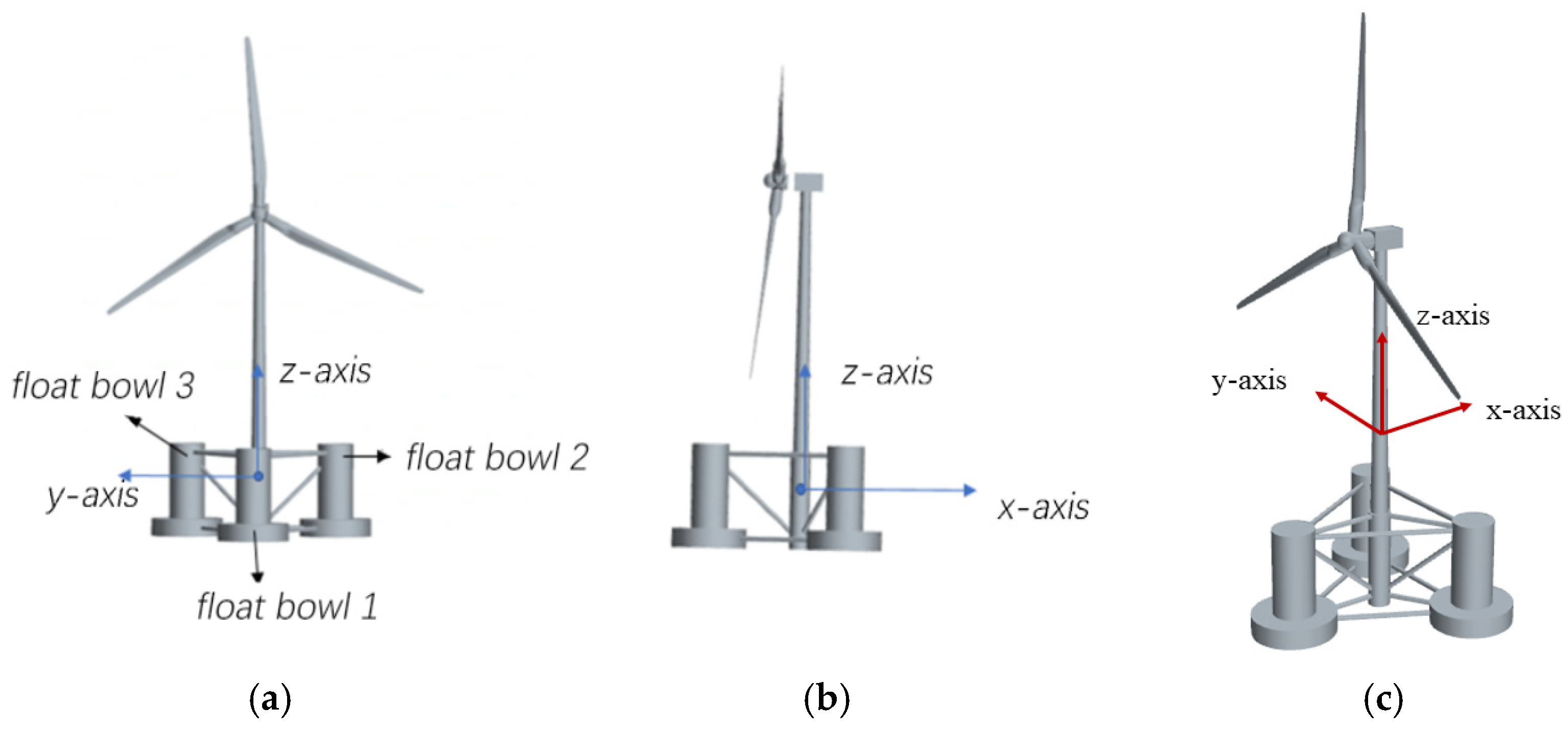
3.1. NREL 5MW FOWT

The NREL 5MW floating offshore wind turbine (FOWT) is selected as the research object in this paper. The structure of the floating wind turbine can be divided into three parts: upper wind turbine structure, tower foundation, and anchor chain mooring. The NREL 5MW wind turbine is a conventional three-blade upwind variable pitch blade wind turbine that was designed by the National Renewable Energy Laboratory of the United States. It is composed of NACA-64 and DU series airfoil. The floating foundation adopts the semi-submersible platform OC4, which is composed of three pontoons and one column in the middle; the pontoons and the column are connected by a truss structure.

Table 1. Main dimensions of NREL 5MW wind turbine.

Project	Parameter
Wheel orientation Number of blades	Upwind Three blades
Wind wheel radius Rotor radius	126 m 3 m
Cut in wind speed Rated wind speed Cut out wind speed	3 m/s 11.4 m/s 25 m/s
Cut in rotational speed Rated rotational speed Cut out rotational speed	6.9 rpm 12.1 rpm 12.1 rpm
Extension Elevation Cone Angle	5 m 5° 2.5°

and

Table 2. Main dimensions of OC4 platform.

Project	Parameter
Draft	20 m
Barycenter (Below the waterline)	13.46 m
Platform mass (Including ballast water)	1.3473 × 107 kg
Height to the top of the tower (Above the waterline)	87.6 m

list the rotor and platform parameters. The three-dimensional model of the floating wind turbine is shown in Figure 2.

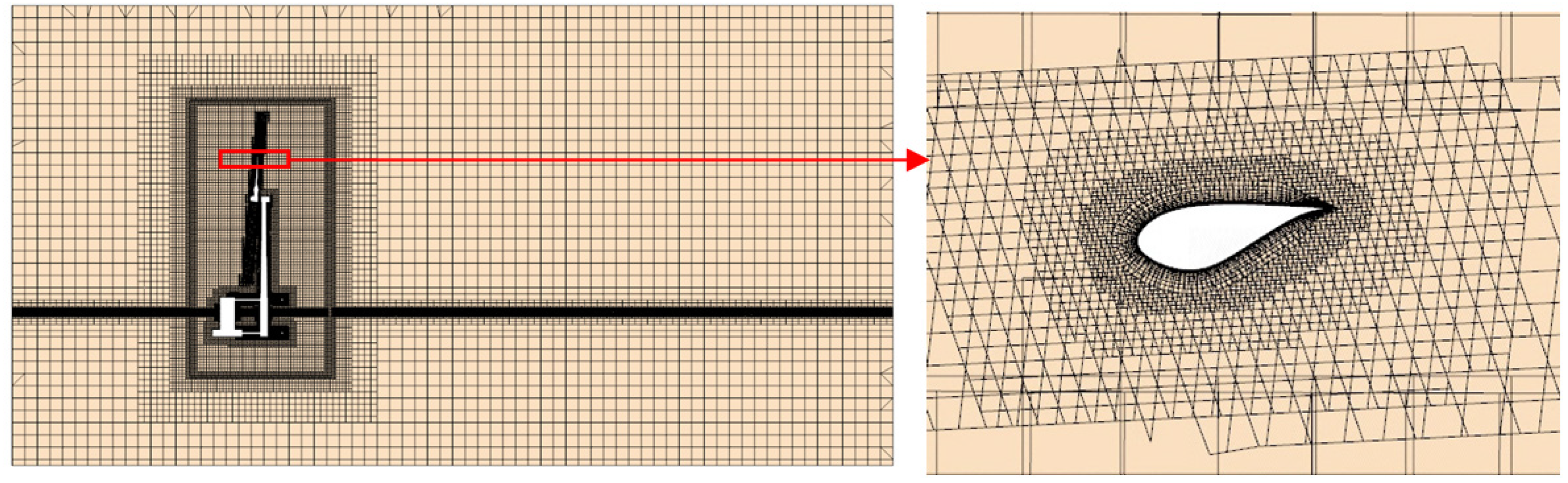
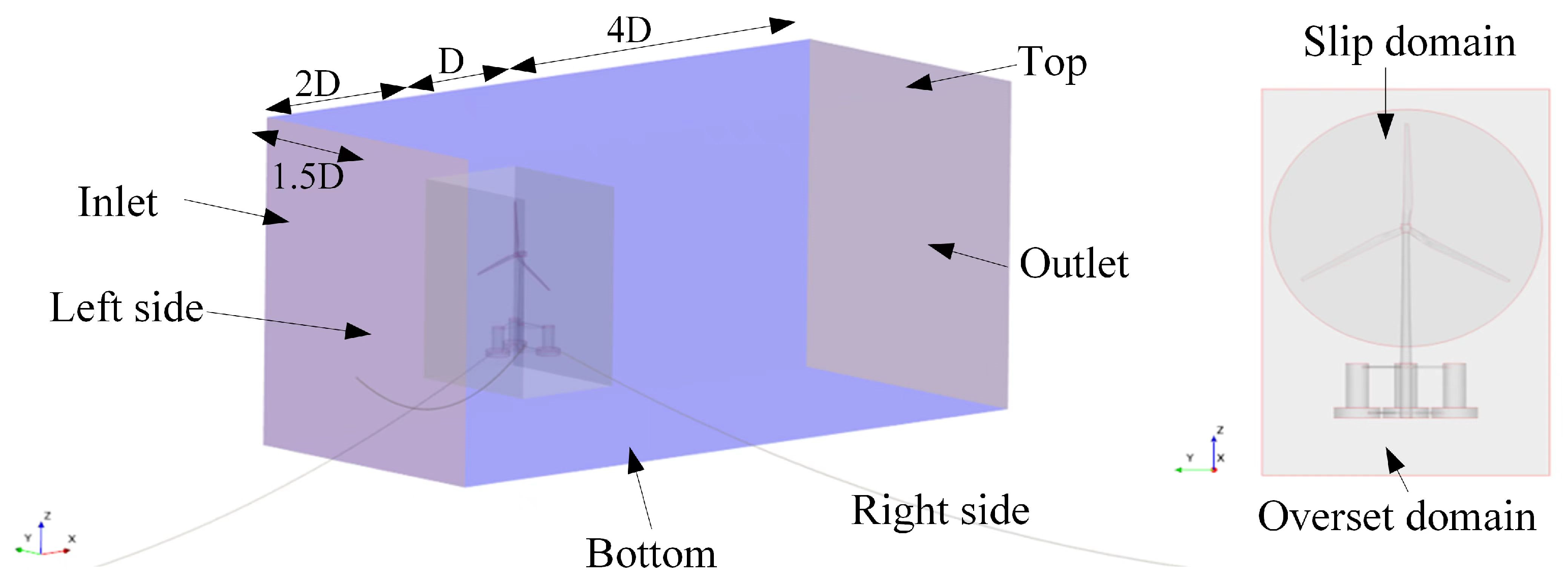
3.2. Setups of the CFD Model

In the coupled CFD–FEA simulation of the floating wind turbine, both the overset mesh and sliding mesh techniques are applied to deal with complex multi-stage motion problems. In the numerical simulation, three sets of meshes are created, including the background domain mesh, the overset mesh, which is used for simulating the six degrees of freedom of the floating wind turbine and tower, and the Multiple Reference Frame (MRF) adopted for the blade rotation. The structured mesh is used for the mesh strategy, and the mesh is generated by the cutting volume mesh and the prismatic layer mesh. The mesh located at the interface between the air and fluid is generated by the surface repair and the surface reconstruction. The refined mesh is adopted on blades and platforms, and also set on the free surface, which is supposed to capture the interface between the wind and wave.

To accurately model the real shape of the floating platform and blades, a mesh control method is added to control the overset meshes in the calculation domain. To evaluate the mesh sensitivity and uncertainty, numerical simulations are carried out with three sets of meshes. The mesh size between each mesh set is $\sqrt{2}$ times. Detailed information for the three sets of meshes and the simulation results for the thrust and the pitch are listed in

Table 3. Detailed information for the three suites of meshes.

Meshes	Mesh Size for Blade (m)	Mesh Size for Platform (m)	The Number of Cells (Million)	Thrust (kN)	Pitch (°)	Computational Cost (Hour)
Mesh1	0.20	0.55	4.98	170.5	1.88	145
Mesh2	0.15	0.48	7.07	172.5	1.98	168
Mesh3	0.10	0.34	9.86	175.2	2.12	235.2
Mesh4	0.08	0.24	11.26	176.3	2.14	271.2

.

Considering the calculation cost and accuracy, the final mesh division scheme is determined. The coarse mesh configuration is employed. The basic mesh size of the background domain is 5 m in the mesh diagram. To ensure that there are at least four overlapping layers between the overlapping mesh and the background domain, the overset mesh size is set to 1 m, and the vertical direction of the free surface is refined and set to 1/25 of the wave height. Figure 3 shows the mesh diagram of the calculation domain in the middle longitudinal section. It can be seen from the table that the value of thrust is about 175 kN, and the pitch angle is around 2°. With the increase of the number of meshes, the calculation results of thrust and pitch angle change a little [23]. In consideration of the computational cost, the Mesh 2 strategy is used in all our numerical simulations.

The horizontal axis floating wind turbine is installed in the offshore region, which suffers from complex external load during its lifetime. In order to simulate the motion of the full-scale model under different conditions, the full-scale NREL 5MW FOWT is imported into the CFD platform STAR-CCM+ to establish the calculation domain and divide the mesh. The calculation domain is divided into background domain, overset domain, and slip domain. The calculation domains and their corresponding boundary conditions are shown in

Table 4. The boundary conditions.

Calculation Domain	Boundary Name	Boundary Condition
Background domain	Inlet	Velocity inlet
	Outlet	Pressure outlet
	Left side	Wall
	Right side	Wall
	Top	Wall
	Bottom	Wall
Overset domain	Platform and tower	Wall
	The interface on the blade rotating and fixed region	Velocity inlet
Rotating Region	The interface on the blade rotating and fixed region	Velocity inlet
	Blade model	Wall

and Figure 4. The inlet is located in the 2D distance from the wind turbine model, the left and right side is located in the distance 1.5D, and the distance from the wind turbine model to the outlet is 5D. A wave suppression area of 1D is set at the outlet to avoid the influence of wall reflection on the fluid. The boundary conditions are set according to the reference [23,24].

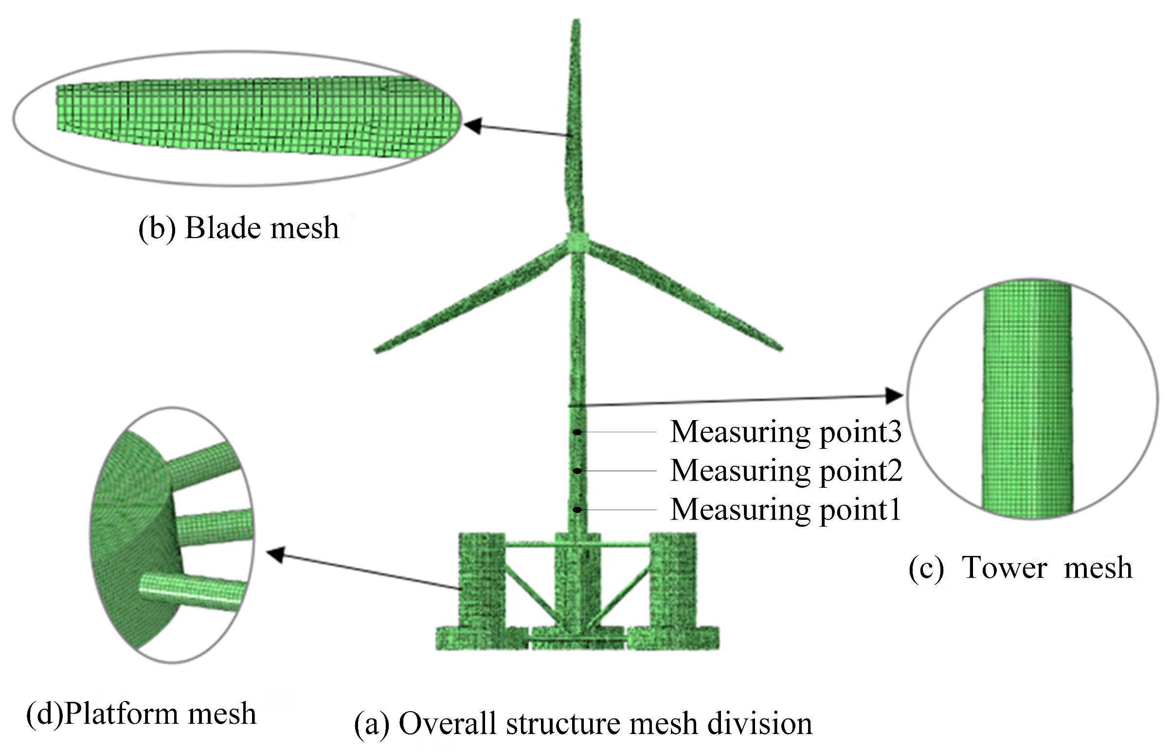
3.3. Setups of the FEA Model

In the CFD-FEA simulation, the structural finite element mesh is set up in the FEA platform. The geometric model of floating wind turbine (including the platform ribs, the stiffener, and the blade web structure) is established in SOLIDWORKS 2022, and then is imported into the mesh division software to complete the mesh division. The mesh and node information are imported into the FEA platform to complete the definition of material parameters and boundary conditions. In order to ensure the correctness of the mesh mapping in the CFD–FEA simulation, the size of the finite element mesh of the structure is similar to that of the hydrodynamic model. The base sizes of the mesh for the blade and the platform are 0.2 m and 0.48 m, respectively. After the division, the total number of mesh cells for the FEA model is 290,000. Figure 5 shows the structural finite element mesh of the floating wind turbine.

In order to explore the stress and deformation of the blade, eight nodes are arranged equidistantly on the blade, as shown in Figure 6.

The structural model is made of fiberglass, and its allowable stress is AH36, which is the same as a general high-strength steel for the platform structure. The yield strength is 355 MPa; when the safety factor is 1.35, the allowable stress is 263 MPa. The material parameters are shown in

Table 5. Material parameters.

Physical Parameter	Fiberglass	AH36
Density (kg × m−3)	1160	7850
Elasticity (GPa)	72	210
Poisson’s ratio	0.42	0.3

.

3.4. Ocean Environmental Parameters

The loads and responses of the NREL 5 MW wind turbine under varying wind speeds, wave heights, and wind wave directions are investigated by the coupled CFD–FEA. According to the wind and wave conditions listed in reference [25], the simulation conditions are set in

Table 6. The wind and wave cases.

Case Number	Type of Condition	Wind Speed (m/s)	Wave Height (m)	Wind/Wave Direction (°)
Case 1	Wind speed	10	3	0
Case 2		15	3	0
Case 3		20	3	0
Case 4		25	3	0
Case 5	Wave height	15	1	0
Case 2		15	3	0
Case 6		15	6	0
Case 2	Direction of the wind and waves	15	3	0
Case 7		15	3	30
Case 8		15	3	60
Case 9		15	3	90

. First, the design of Cases 1–4 lies in investigating the effects of the wind speed on the FOWT. Because when the wind speed exceeds 25 m/s, the wind turbine will stop rotating to prevent damage to the blade structure, as this is the cut-out wind speed, it is set to 10 m/s, 15 m/s, 20 m/s, and 25 m/s, respectively, in Cases 1–4. Meanwhile, the wave height and the wind/wave direction are set to 3 m and 0, respectively, and kept unchanged in the four cases. Second, the design of Cases 2, 5, and 6 lies in investigating the effects of the wave height on the FOWT. The wave height is set to 1 m, 3 m, and 6 m. The period is specified as 8 s, and the wind speed remains unchanged at 15 m/s. The regular wave is adopted in all the simulations. Finally, considering the actual conditions of wind and wave disorientation in the deep sea, the design of Cases 2, 7, 8, and 9 lies in investigating the effects of the direction of the wind and waves on the FOWT. The direction of wave changes from 0° to 90° at intervals of 30°, the wind speed is kept unchanged as 15 m/s, and the wave height is set to 3 m. The effect of the wave period is not considered in this paper; thus, the wave period is set to 8 s. There is no controller used for the turbine; the specified parameters are set as Table 1.

4. Results and Discussion

In this section, the analysis for the time-domain results of the motion response and the structural responses of the NREL 5 MW floating wind turbine for Case 2 are first presented in Section 4.1 and Section 4.2. Then, the effects of the following three ocean environmental parameters, including the wind speed, the wave height, and the wind/wave direction, on the structural responses are systematically presented and discussed in Section 4.3, Section 4.4 and Section 4.5, respectively.

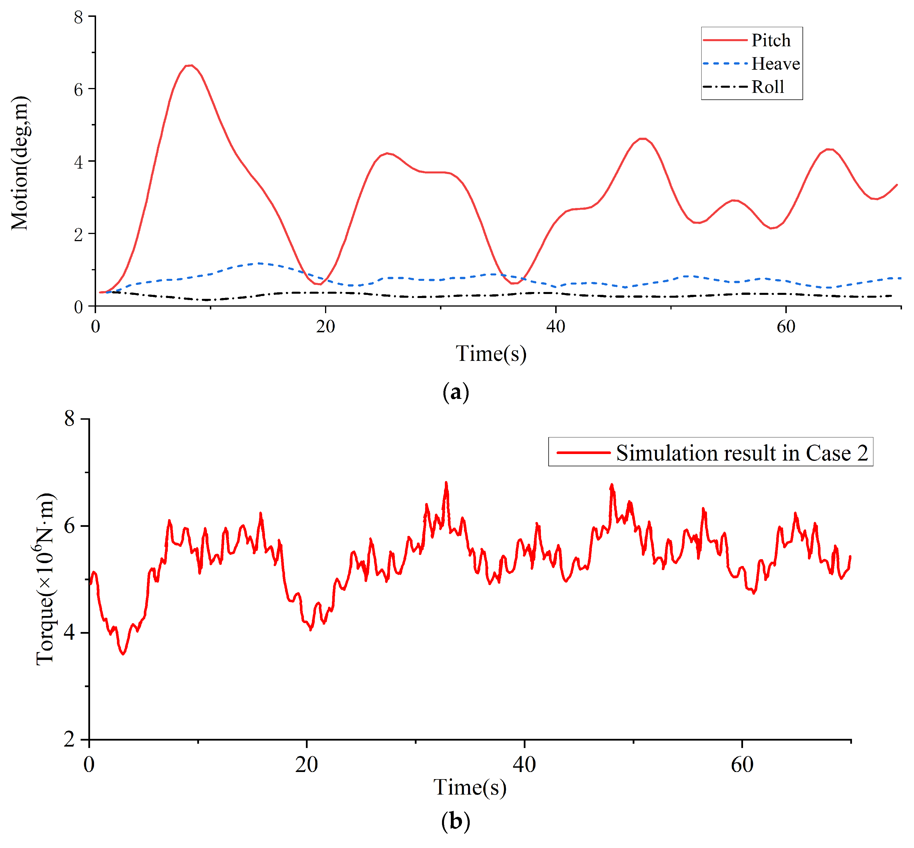
4.1. Analysis of Motion Characteristics of Case 2

Through the CFD–FEA coupling approach described above, the motion of the floating wind turbine, the load of the blade, the structural deformation and stress under various wind speeds, the wave heights, and the wind/wave directions can be estimated. In this subsection, the simulated time-domain results on the motion of the floating wind turbine and the load of the blade for Case 2 are presented.

Figure 7 shows the velocity distribution of the flow field when the wind speed is 15 m/s. Figure 7a illustrates the velocity contour of the flow field at the y = 0 plane. The wind speed decreases significantly after passing through the plane of rotation of the wind turbine, which is attributed to the blocking effect of the blade and tower on the incoming airflow. The wind turbine absorbs a portion of the wind energy and converts it from mechanical energy into electrical energy. Meanwhile, the remaining portion creates a wake area as it passes through the wind turbine. Due to the combined effects of wind and waves, the wind turbine experiences noticeable pitching motion. The interaction between the wake and the wave and the movement of the floating wind turbine disrupts the flow field. Figure 7b depicts the velocity contour of the flow field with the blade. In the rotation process of the wind turbine, a high-speed rotation domain is formed at the tip of the blade and the guide edge of the blade, but the blade velocity decreases significantly along the edge, which proves that the pressure difference here is larger and the blade is subjected to greater load. Figure 7a shows the movement of the platform, which presents periodic changes under the influence of wind and waves. After the first cycle, the movement tends to be stable.

The time-domain curve of the motion of the floating wind turbine is shown in Figure 8. It is seen that the motion of the floating wind turbine is noticeable in the wind and wave fields. The response period of the movement of the floating wind turbine is 8 s; thus, the wave period that equals 8 s is used in all the conditions. When the first wave hits the floating wind turbine, it causes the support platform to move forward along the x-axis due to the wave force and further results in noticeable pitch and heave motions. When the surge motion reaches its maximum, the mooring line’s opposing force begins to move in the negative x-axis direction until the equilibrium position is reached, and periodic wave frequency motion is performed at that position. The final balance position of the pitch angle is about 4.3°. The time-domain curve of the movement of the floating wind turbine is shown in Figure 8a. Figure 8b is the time-domain curve of torque of the floating wind turbine. It is found that the amplitude of thrust and torque amplitudes exhibit significant vibration and periodic fluctuation. Under this condition, the maximum torque is 7.0 × 10⁶ N·m, the average torque is 5.02 × 10⁶ N·m, the maximum thrust is 882 kN, and the average thrust is 802 kN. As listed in

Table 7. The torque and thrust on the floating wind turbine compared to reference [26].

	Rigid	Flexible	The Averaged Value in Case 2	The Error between the Flexible and the Result of Case 2
Thrust [kN]	780	808	802	0.74%
Torque [kN·m]	4373	4469	4857	8.68%

, the thrust in the reference [24,26], rigid and flexible conditions are 790 kN and 808 kN, which are similar to the averaged thrust in Case 2. The torque in the reference [26], flexible condition is 4.3 × 10⁶ N·m, which is close to the averaged torque in Case 2. The blades are assumed as flexible structure in Case 2; thus, it is close to the results in the reference [26] within the flexible condition. The comparisons of the thrust between the reference [26] and the result of Case 2 are listed in Figure 8c. The difference of the averaged thrust between the reference [26] and the result of Case 2 is less than 10%, which can fully meet the demands of the engineering applications. It is assumed as the validation for the simulation method; thus, this method can be used for the following investigation.

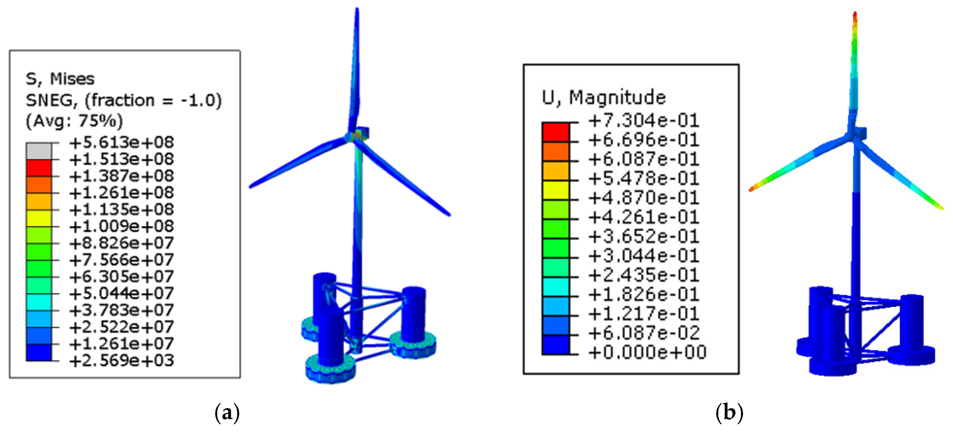
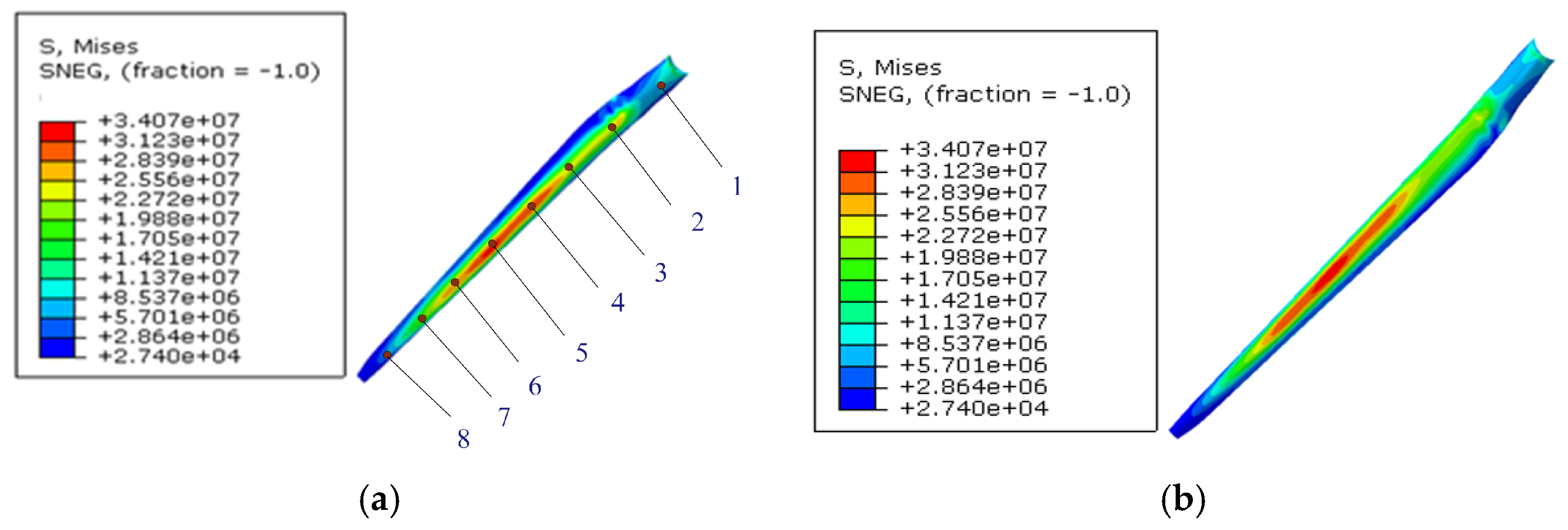
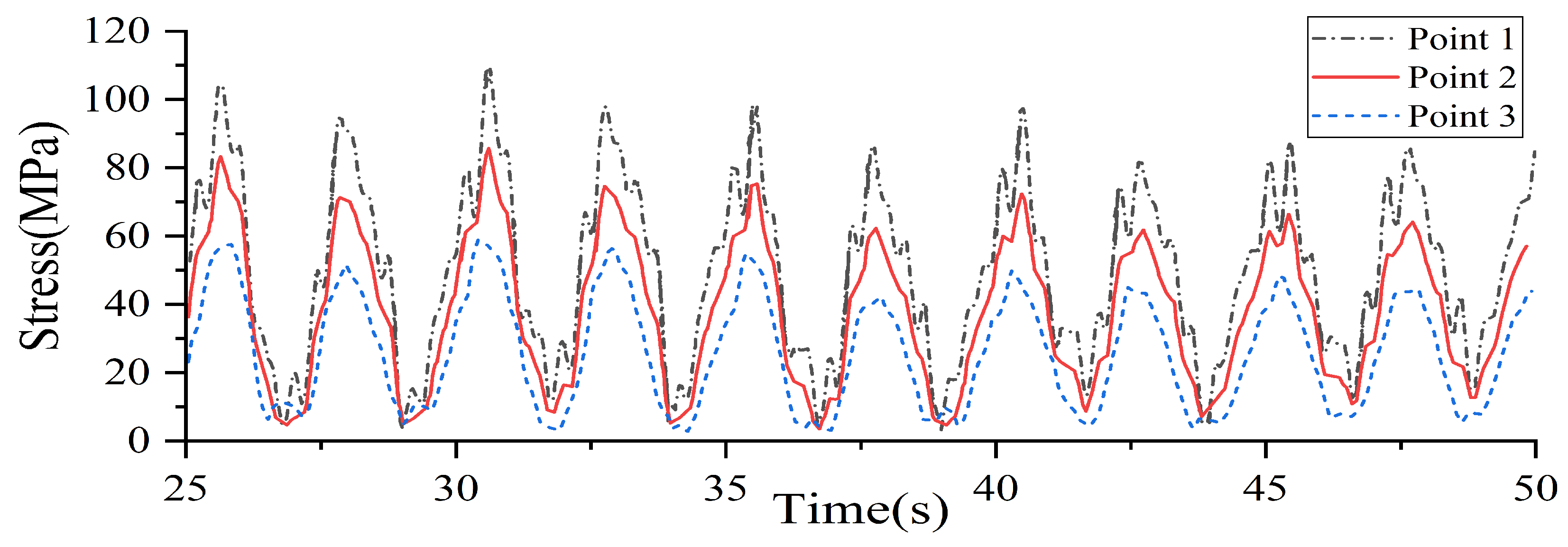
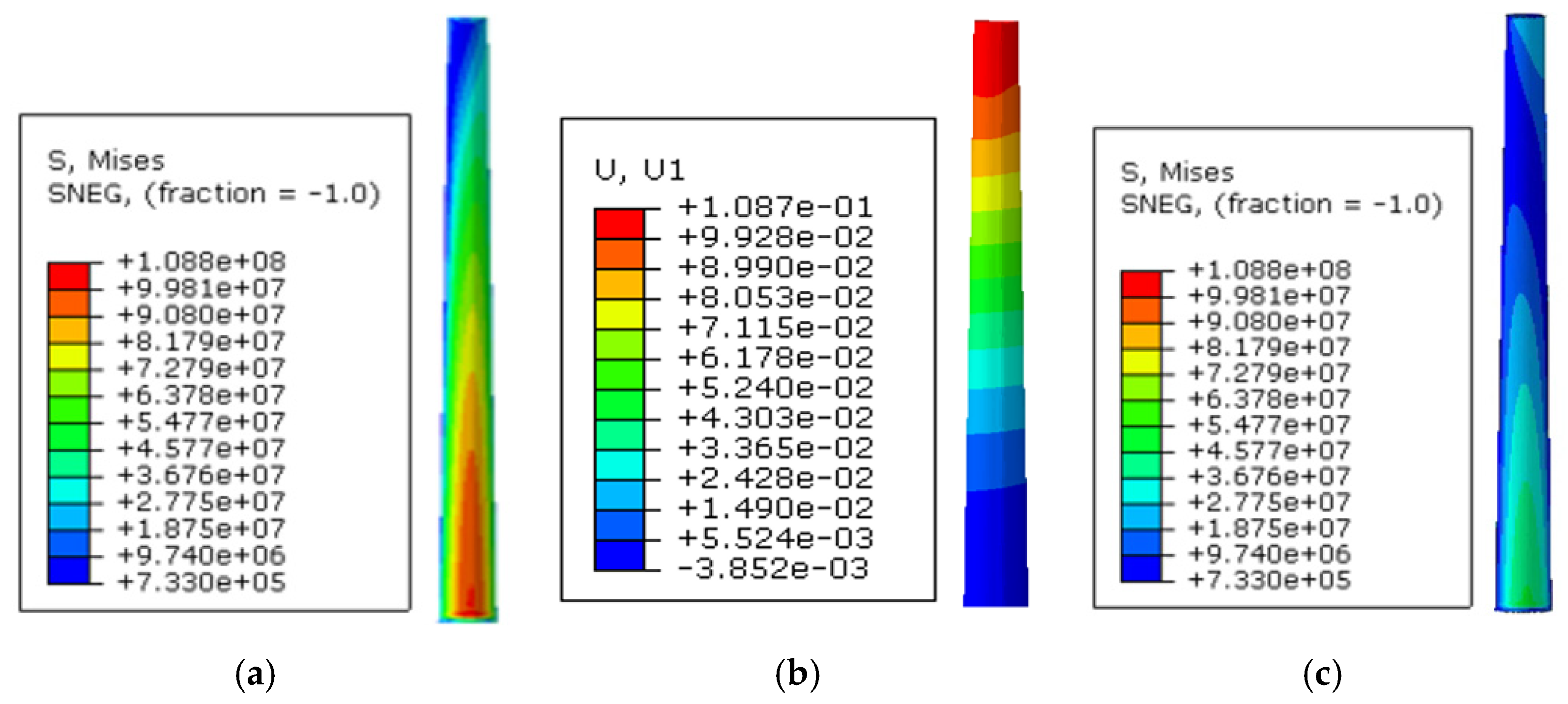
4.2. Analysis of Structural Responses of Case 2

Figure 8 depicts the stress cloud diagram and displacement cloud diagram of the entire structure at a specific time. It can be seen from the stress nephogram (Figure 9a) that the semi-submersible OC4 platform is subjected to greater stress due to the wave load compared to the blade due to the wind load. From the displacement nephogram (Figure 9b), it can be seen that the blade and the tip of the tower exhibit larger deformation compared to the semi-submersible platform, indicating their higher flexibility. The main deformation occurs in the x-axis direction, which is the direction of wind and wave flows, and in the brandishing direction for the blade. The specific structural response analysis will be conducted for individual blades, towers, and platforms below.

It can be seen from the stress distribution (Figure 10a,b) that the maximum equivalent stress and deformation occur at r/R = 0.2~0.8 from the middle of the blade, regardless of the windward and leeward sides. This is the location where the bending moment is primarily sustained, and the maximum stress reaches 3.4 × 10⁷ Pa. In addition, the circular airfoil at the blade root and the DU40 series transition also exhibit obvious stress, which is caused by excessive changes in geometric curvature in this area.

The stress on points 1, 4, and 7 on the blade is analyzed in the time-domain curve (the location of the points is shown in Figure 6). Since the velocity near the waves is different from higher up and the blades pass the tower, the stress on the blades also undergoes periodic changes, as illustrated in Figure 11. The stress value at point 4 shows the most significant change, indicating that this is the location where the primary bending moment is experienced.

Figure 12 presents the time-domain curves of stress of the tower barrel (i.e., at points 1, 2, and 3). Due to the action of waves and wind, as well as the rotation of the three blades, the stress undergoes periodic changes. The tower barrel is a slender and flexible structure. Hence, it will exhibit noticeable structural deformation. As shown in Figure 13, the tower barrel’s displacement increases with height, and the most significant deformation occurs at the top.

Figure 14 presents the time-history curve of the deformation in the x-, y-, and z-axis directions at the top of the tower. The deformation curve presents regular changes, with the smallest deformation in the z-axis direction. It is mainly reflected in the displacement in the x-axis direction, with the maximum deformation reaching 0.13 m. The maximum stress of the tower is 108.8 MPa, which is lower than the allowable stress of 263 MPa, meeting the strength requirement.

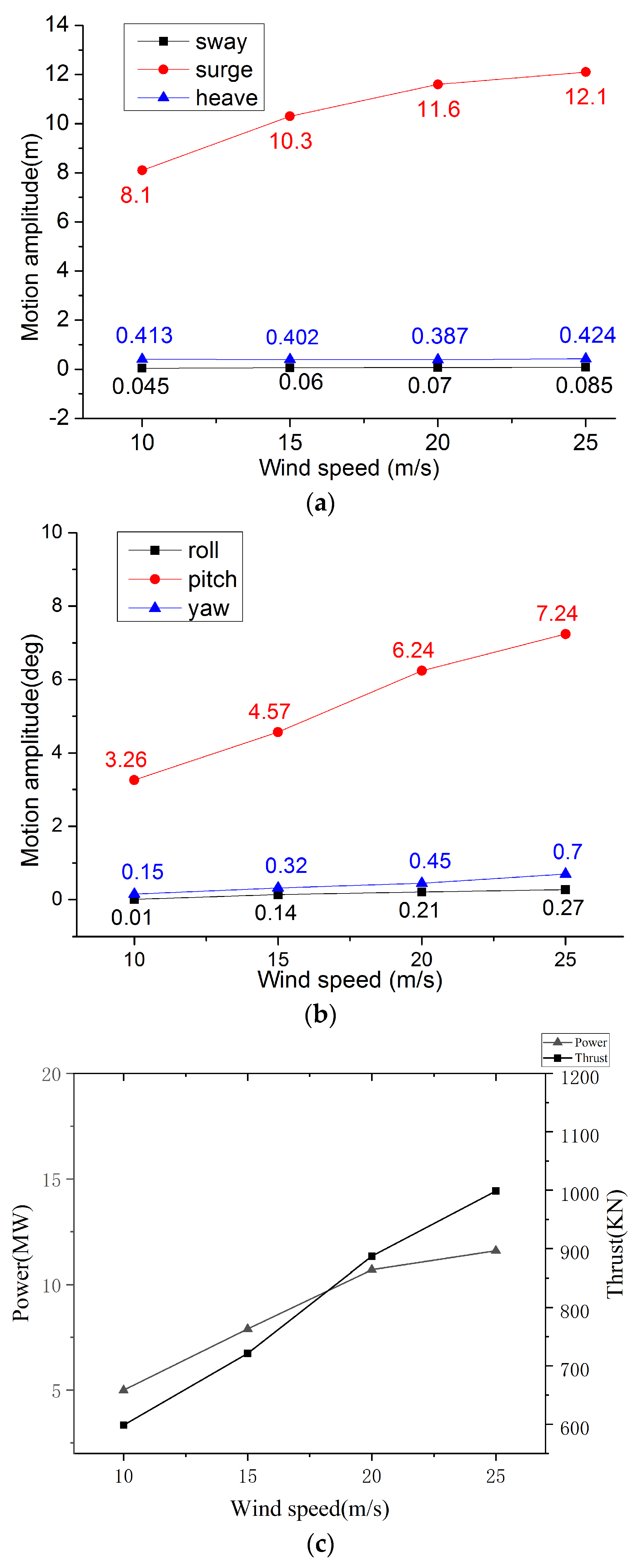
4.3. Wind Speed Effect on Motions and Structural Responses

This subsection analyzes and discusses the motion and deformation responses on the floating wind turbine under various wind speeds (corresponding to Cases 1–4 at Table 6). Figure 15 shows the variations of the 6-DOF motion amplitudes of the floating wind turbine with respect to the wind speed. As shown in Figure 15, pitch, roll, and yaw increase with the wind speed, while heave does not change significantly. Among the three translational degrees of freedom, the motion in the x-direction is the most noticeable, and the change in pitch angle is the most obvious among the three rotational degrees of freedom. The wind speed significantly affects the thrust and power of the floating wind turbine, as depicted in Figure 15c. When the pitch angle changes and the wind speed increases to a certain value, the torque will no longer increase and will stabilize, while the thrust will no longer increase but will begin to decrease.

The blade will deform under the incoming flow, with the primary component being flapping deformation in the x-axis direction, as illustrated in Figure 16a,b. Under different wind speeds, the deformation pattern of the blade along the spanwise remains consistent, increasing in a parabolic shape until the deformation at the blade tip reaches its maximum. When the deformation of the blade tip is less than the distance between the tower and the initial blade tip, the blade will not collide with the tower. At the same time, it can be concluded that the slope of the curve increases at the spanwise direction of 10 m, indicating a rapid increase in deformation. This area is where stress growth occurs. This is the section where the maximum bending moment is experienced.

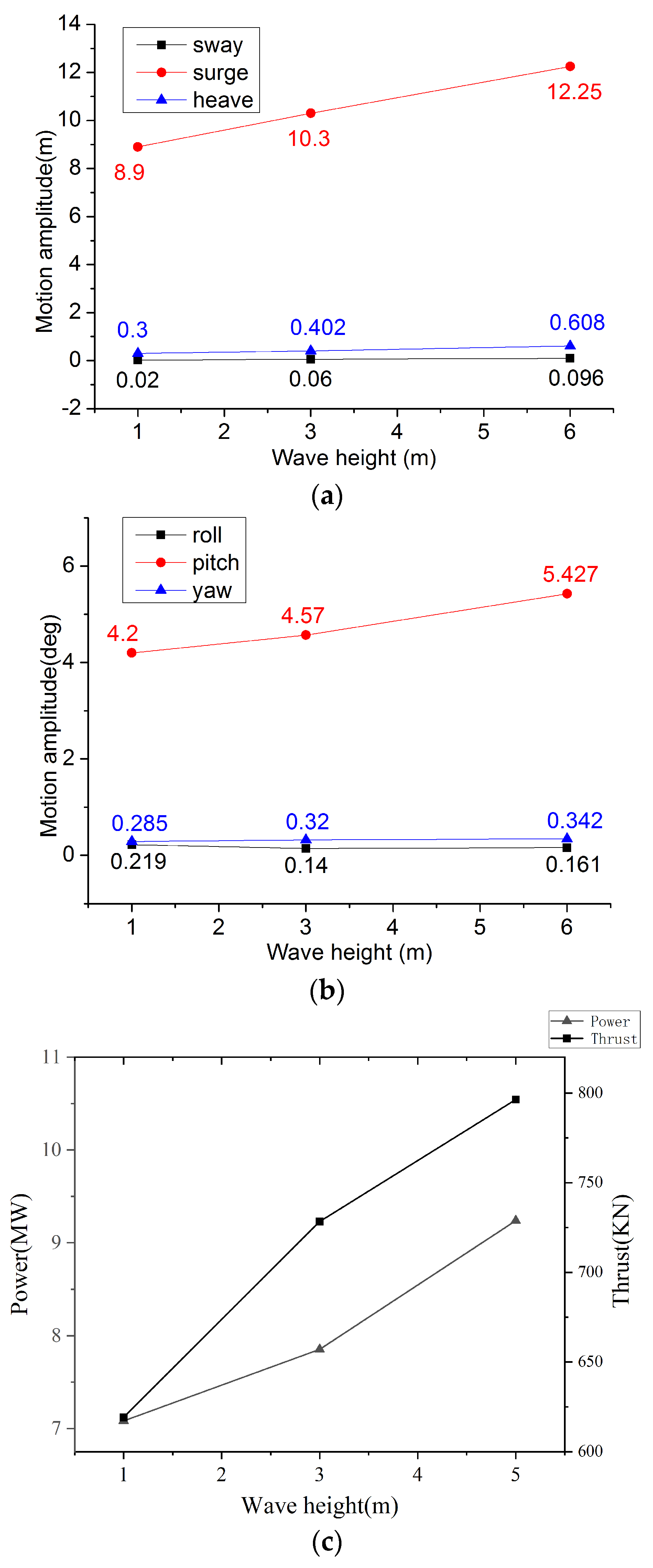
4.4. Wave Height Effect on Motions and Structural Responses

In addition to being affected by wind load, the floating foundation is also subject to wave load, which can impact the structural response of the entire system. This section analyzes the wave loads and motions of the floating wind turbine under different wave heights, namely Case 2, Case 5, and Case 6. Figure 17 shows the 6-DOF motion and thrust under different wave heights in time-domain results. The heave motion is more intense among the three translational degrees of freedom. This is similar to the impact of wind speeds on the dynamic response of the floating wind turbine. Figure 17c lists the variations in wind turbine thrust and output power at different wave heights. It can be observed that, under the same wind speed and varying wave heights, both the output power and thrust of the wind turbine exhibit an increasing trend.

Figure 18a depicts the stress of blades along the spanwise with different wave heights. The stress is observed to be highest in the middle region of the blades, specifically in the 20–80% range, which follows the same variation pattern as the simulations conducted under different wind speeds. When the wave height is 1 m, the maximum equivalent stress is 32.3 MPa. When the wave height is 6 m, the maximum equivalent stress on the blade is 36.1 Mpa. Figure 18b depicts the deformation patterns of the blade tip along the spanwise direction with different wave heights. Both patterns exhibit a parabolic form, with the blade tip deformation reaching its maximum value. As the wave height increases, the maximum blade deformation also increases. When the wave height is 1 m, the maximum blade tip deformation is 0.67 m. When the wave height is 6 m, the maximum blade tip deformation is 1.63 m. Due to the increase in wave height, the incidence angle of the wind is affected by platform pitch changes. Consequently, the aerodynamic performance of each section of the blade also changes, even though the wind speed remains unchanged. The aerodynamic performance affects the elasticity of the blade, resulting in changes in blade deformation and maximum equivalent stress. Similar to the rule for varying wind speed conditions, the middle of the blade experiences a significant bending moment. Therefore, it is essential to consider the strength of this area when designing the blade.

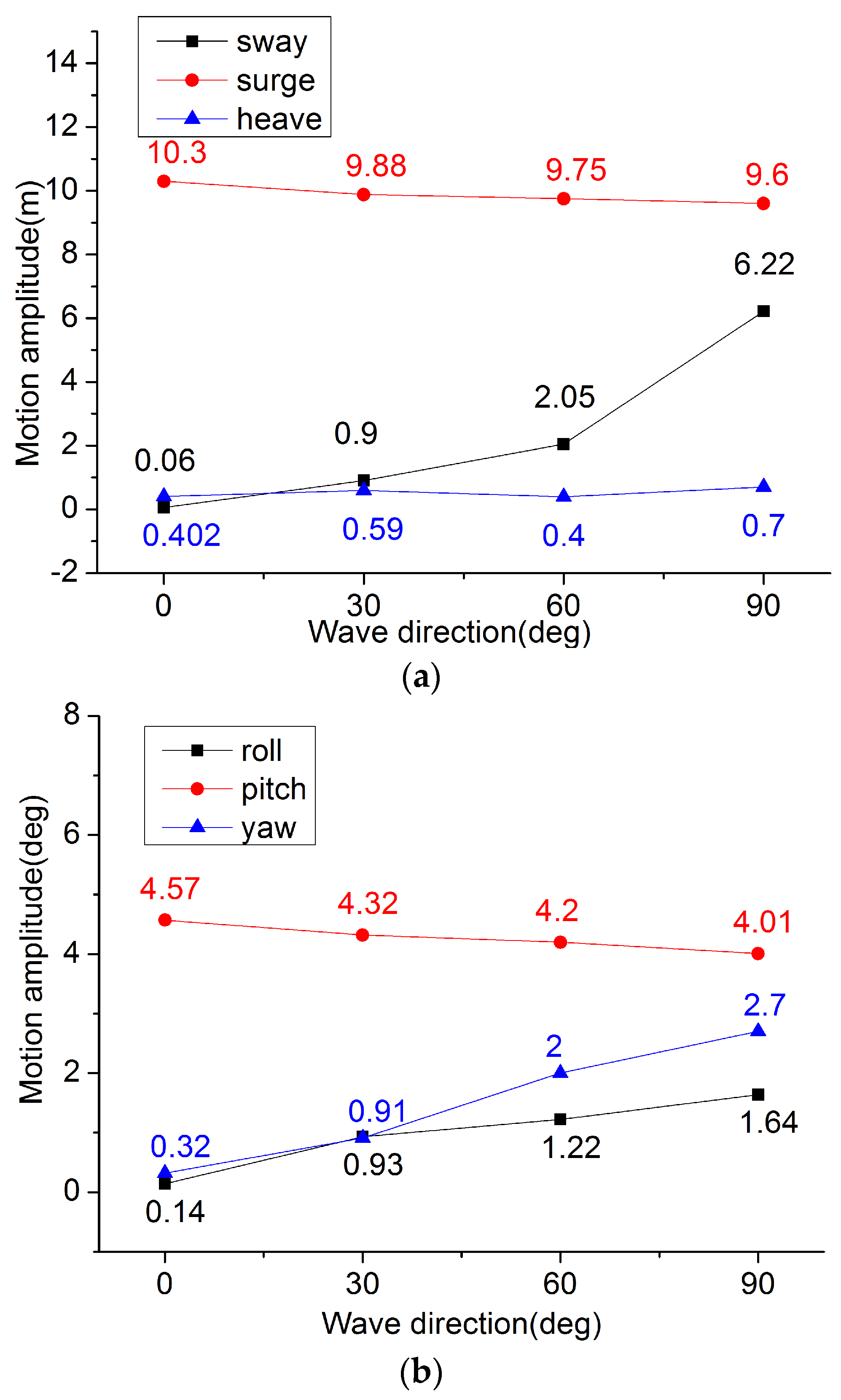
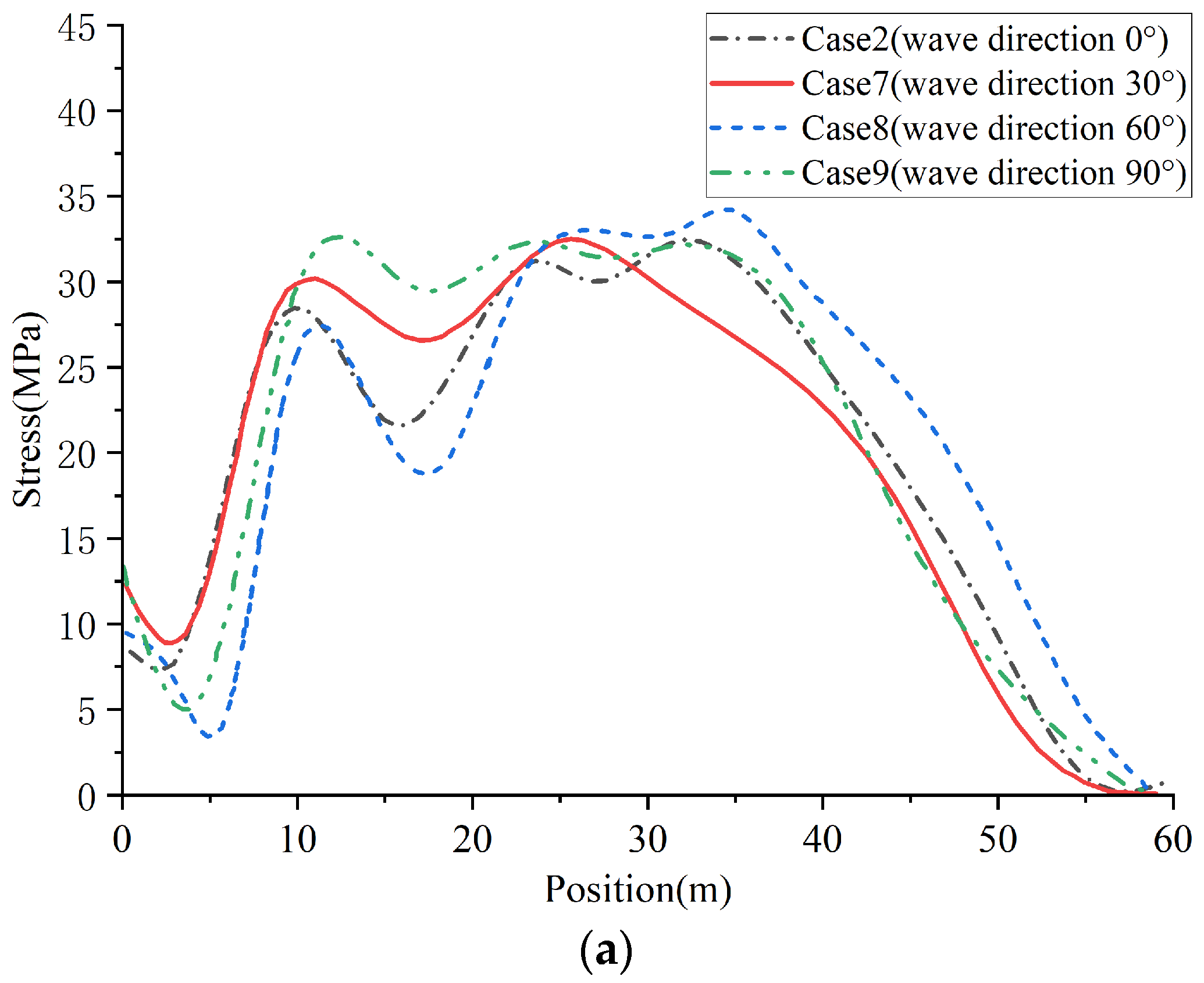
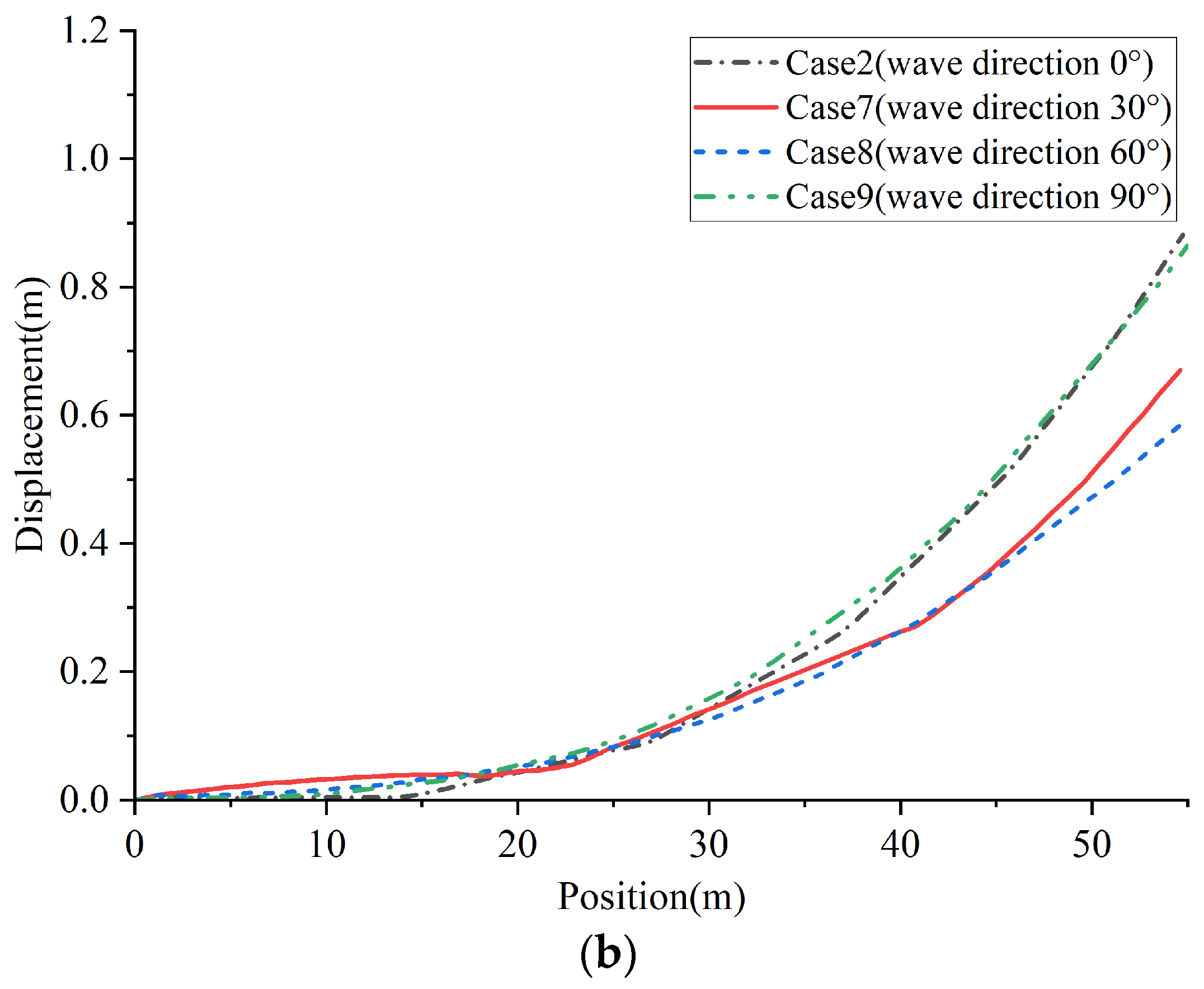
4.5. Wind/Wave Direction Effect on Motions and Structural Responses

During the operation of a floating wind turbine at sea, it will be subjected to the combined action of wind, waves, and various loads. The wind and waves are not always in the same direction; there is a certain angle between the wave direction and wind direction. This section examines the impact of varying wind and wave directions on the load and structural response of the floating wind turbine. The wind speed is 15 m/s, the wave height is 3 m, the wind direction remains unchanged, and the wave’s dislocation angle changes within the range of 0° to 90°.

The results of Case 2, Case 7, and Case 8 are analyzed in this section. Figure 19 illustrates the 6-DOF motion and thrust of the floating wind turbine under various wave directions. At 0°, the wave experiences the maximum load in the surging direction. As the wave incidence angle increases, the wave load in the surging direction gradually decreases. Heave motion is almost unchanged, while roll motion is the most sensitive to changes in wave direction. At wave direction 90°, the roll motion is 6.22 m; the yaw angle also reaches 2.7°. It is evident that the change in wave direction significantly affects the lateral movement of the floating wind turbine. Figure 19c illustrates the thrust and output power of the floating wind turbine in varying wave directions. At the same wind speed and wave height, the output power and thrust of the wind turbine do not change significantly. The output power of the floating wind turbine remains stable at 7.6 MW, and the thrust is constant at 720 kN.

Figure 20 illustrates the stress and deformation of the blade along the spanwise direction under different wave directions. When the wave direction is 60°, the maximum equivalent stress on the blade is 34.6 MPa. While the change in wave direction does impact blade stress to some extent, it is not as significant as wind speed in affecting the distribution of transverse stress and blade deformation. Under various wave directions, the blade deforms in a parabolic manner along the spanwise direction. The maximum blade tip deformation did not change significantly and remains stable at approximately 0.8 m. According to the above sections, pitch and surge motion have the greatest influence on the aerodynamic performance of the platform. Wind speed plays a significant role in the equilibrium position of pitch and surge. Although the wave direction changes, the aerodynamic performance of each section of the blade does not change significantly. The impact of blade deformation and maximum equivalent stress is not substantial. Similarly, under varying wind speed conditions, the middle of the blade experiences a significant bending moment. Therefore, it is essential to pay attention to the strength of this area when designing the blade.

5. Conclusions

In this paper, a coupled CFD–FEA approach is proposed and applied to predict the motion and deformation responses of the NREL 5MW FOWT with a mooring system. The RANS model and the VOF method are employed, respectively, to generate the water/air two-phase flows and to capture the interface of air and water. The dynamic fluid–body interaction (DFBI), the overset mesh method, and the sliding mesh interface technique are conducted to calculate the fluid load and the structural motion. The explicit nonlinear dynamic FEM method is used to evaluate the deformation response of the structure. Thus, the multi-physical dynamics, which includes hydrodynamics, aerodynamics, and structural dynamics, is taken into account for all the simulations with various wind speeds, wave heights, and wind/wave directions. Based on the present research results, three main conclusions can be drawn:

(1) The wind speed is found to be the main factor affecting the balance position of pitch and pitch, the wave height mainly affects the surge and pitch motion of the floating wind turbine, and the wind/wave direction mainly affects the lateral motion of the floating wind turbine.

(2) Under different simulation conditions, the maximum stress position of the blade appears in the middle of the blade and the transition of the blade root.

(3) Under different environmental conditions, the maximum stress position of the blade appears in the middle of blade and the transition between blade root and air foil. The stress of the platform increases with the wave height, and the maximum stress of the floating wind turbine is most significantly correlated with the wave height. The maximum stress of the whole structure occurs at the place where the strut is connected with the column or the buoy.

References

1. Global Offshore Wind Report. 2022. Available online: https://www.gwec.net/ (accessed on 13 July 2024).
2. Roddier, D.; Cermelli, C.; Aubault, A.; Weinstein, A. WindFloat: A floating foundation for offshore wind turbines. J. Renew. Sustain. Energy 2010, 2, 033104. [Google Scholar] [CrossRef]
3. Robertson, A.; Jonkman, J.; Masciola, M.; Song, H.; Goupee, A.; Coulling, A.; Luan, C. Definition of the Semisubmersible Floating System for Phase II of OC4; NREL Technical Report; NREL/TP-5000-60601; National Renewable Energy Lab. (NREL): Golden, CO, USA, 2014. [CrossRef]
4. Arramach, J.; Boutammachte, N.; Bouatem, A.; Mers, A.A. Prediction of the Wind Turbine Performance by Using a Modified BEM Theory with an Advanced Brake State Model. Energy Procedia 2017, 118, 149–157. [Google Scholar] [CrossRef]
5. Jonkman, J.; Butterfield, S.; Musial, W.; Scott, G. Definition of a 5-MW Reference Wind Turbine for Offshore System Development; NREL Technical Report; NREL/TP-500-38060; National Renewable Energy Lab. (NREL): Golden, CO, USA, 2009. [CrossRef]
6. Jonkman, J. Dynamics of offshore floating wind turbines-model development and verification. Wind Energy 2010, 12, 459–492. [Google Scholar] [CrossRef]
7. Masciola, M.; Robertsen, A.; Jonkman, J.; Driscoll, F. Investigation of a FAST-OrcaFlex Coupling Module for Integrating Turbine and Mooring Dynamics of Offshore Floating Wind Turbines. In Proceedings of the 2011 International Conference on Offshore Wind Energy and Ocean Energy, Beijing, China, 31 October–2 November 2011. [Google Scholar]
8. Wu, J. Numerical Simulation of Aerodynamic Performance of Offshore Floating Wind Turbine; Shanghai Jiao Tong University: Shanghai, China, 2016. (In Chinese) [Google Scholar]
9. Li, P.; Wan, D.; Hu, C. Fully-Coupled Dynamic Response of a Semi-submerged Floating Wind Turbine System in Wind and Waves. In Proceedings of the 26th International Ocean and Polar Engineering Conference, Rhodes, Greece, 26 June–2 July 2016. [Google Scholar]
10. Liu, Y.; Xiao, Q.; Incecik, A.; Peyrard, C.; Wan, D. Establishing a fully coupled CFD analysis tool for floating offshore wind turbines. Renew. Energy 2017, 112, 280–301. [Google Scholar] [CrossRef]
11. Cheng, P.; Huang, Y.; Wan, D. A numerical model for fully coupled aero-hydrodynamic analysis of floating offshore wind turbine. Ocean Eng. 2019, 173, 183–196. [Google Scholar] [CrossRef]
12. Srensen, N.; Michelsen, J.; Schreck, S. Navier–Stokes predictions of the NREL phase VI rotor in the NASA Ames 80 ft × 120 ft wind tunnel. Wind Energy 2002, 5, 151–169. [Google Scholar] [CrossRef]
13. Quallen, S.; Tao, X.; Carrica, P.; Li, Y.; Xu, J. CFD Simulation of a Floating Offshore Wind Turbine System Using a Quasi-Static Crowfoot Mooring-Line Model. In Proceedings of the 23rd International Ocean & Polar Engineering Conference, Anchorage, AK, USA, 30 June–5 July 2013. [Google Scholar]
14. Rentschler, M.; Handramouli, P.; Vaz, G.; Vire, A.; Goncalves, R.T. CFD code comparison, verification and validation for decay tests of a FOWT semi-submersible floater. J. Ocean. Eng. Mar. Energy 2023, 9, 233–254. [Google Scholar] [CrossRef]
15. Li, X.; Xiao, Q.; Wang, E.; Peyrard, C.; Gonçalves, R.T. The dynamic response of floating offshore wind turbine platform in wave-current condition. Phys. Fluids 2023, 35, 087113. [Google Scholar] [CrossRef]
16. Gonçalves, R.T.; Chame, M.E.F.; Silva, L.S.P.D.; Koop, A.; Suzuki, H. Experimental flow-induced motions (FIM) of a FOWT semi-submersible type (OC4 phase II floater). J. Offshore Mech. Arct. Eng. 2021, 143, 012004. [Google Scholar] [CrossRef]
17. Miao, W. Study on Fluid-Structure Interaction Response of Wind Turbine and Adaptive Wind Resistance of Blades under Typhoon Environment; University of Shanghai for Science and Technology: Shanghai, China, 2019. (In Chinese) [Google Scholar]
18. Yan, J.; Korobenko, A.; Deng, X.; Bazilevs, Y. Computational free-surface fluid-structure interaction with application to floating offshore wind turbines. Comput. Fluids 2016, 141, 155–174. [Google Scholar] [CrossRef]
19. Dobrev, I.; Massouh, F. Fluid-structure interaction in the case of a wind turbine rotor. In Proceedings of the 18ème Congrès Français de Mécanique, Grenoble, France, 27–31 August 2007. [Google Scholar]
20. Korobenko, A.; Yan, J.; Gohari, S.; Sarkar, S.; Bazilevs, Y. FSI Simulation of two back-to-back wind turbines in atmospheric boundary layer flow. Comput. Fluids 2017, 158, 167–175. [Google Scholar] [CrossRef]
21. Liu, W.; Luo, W.; Yang, M.; Xia, T.; Huang, Y.; Wang, S.; Leng, J.; Li, Y. Development of a fully coupled numerical hydroelasto-plastic approach for offshore structure. Ocean Eng. 2022, 258, 111713. [Google Scholar] [CrossRef]
22. Luo, W.; Liu, W.; Chen, S.; Zou, Q.; Song, X. Development and Application of an FSI Model for Floating VAWT by Coupling CFD and FEA. J. Mar. Sci. Eng. 2024, 12, 683. [Google Scholar] [CrossRef]
23. ASME V&V 20-2009; Standard for Verification and Validation in Computational Fluid Dynamics and Heat Transfer. American Society of Mechanical Engineers: New York, NY, USA, 2009.
24. Jiao, J.; Huang, S.; Tezdogan, T.; Terziev, M.; Soares, C.G. Slamming and green water loads on a ship sailing in regular waves predicted by a coupled CFD–FEA approach. Ocean Eng. 2021, 241, 110107. [Google Scholar] [CrossRef]
25. The Grade of Wind Speed; Maritime Safety Administration of the People’s Republic of China: Beijing, China, 2017.
26. Imiela, M.; Wienke, F.; Rautmann, C.; Wilberg, C.; Hilmer, P.; Krumme, A. Towards Multidisciplinary Wind Turbine Design Using High- Fidelity Methods. In Proceedings of the 33rd Wind Energy Symposium, Kissimmee, FL, USA, 5–9 January 2015; pp. 1–12. [Google Scholar]
Figure 1. The scheme of the one-way coupling approach.
Jmse 12 01385 g001
Figure 2. The floating wind turbine. (a) The front view; (b) the side view; (c) the oblique view.
Jmse 12 01385 g002
Figure 3. The mesh diagram of the calculation domain.
Jmse 12 01385 g003
Figure 4. The boundary condition of the calculation domain.
Jmse 12 01385 g004
Figure 5. The mesh diagram of the structural finite element mesh.
Jmse 12 01385 g005
Figure 6. The distribution of the nodes.
Jmse 12 01385 g006
Figure 7. The velocity distribution of the flow field in case of wind speed = 15 m/s. (a) Velocity distribution in y = 0 m; (b) velocity distribution with the blade.
Jmse 12 01385 g007
Figure 8. The motion, torque, and thrust of the floating wind turbine in Case 2. (a) The motion of the platform; (b) the time-domain curves of torque of the floating wind turbine; (c) the comparisons between Imiela 2013 [26] and the simulation result of thrust.
Jmse 12 01385 g008aJmse 12 01385 g008b
Figure 9. The stress cloud diagram and deformation cloud diagram of the FWOT. (a) The stress nephogram; (b) the deformation nephogram.
Jmse 12 01385 g009
Figure 10. The stress of the blade. (a) The windward side; (b) the leeward side.
Jmse 12 01385 g010
Figure 11. The time-domain curves of stress of the blade.
Jmse 12 01385 g011
Figure 12. The time-domain curves of the stress of the tower barrel at points 1–3.
Jmse 12 01385 g012
Figure 13. The stress and deformation of the tower barrel. (a) Windward side; (b) leeward side; (c) deformation.
Jmse 12 01385 g013
Figure 14. The time-domain curves of the total deformation and the deformations at the three axis directions of the tower top.
Jmse 12 01385 g014
Figure 15. The 6-DOF motion amplitudes of the floating wind turbine under wave height 3 m, wave period 8 s, wave direction 0. (a) The sway, surge, heave of the floating wind turbine; (b) the roll, pitch, yaw of the floating wind turbine; (c) the thrust of the floating wind turbine.
Jmse 12 01385 g015
Figure 16. The stress and displacement of the blade along the spanwise direction of Case 1, 2, 3 and 4. (a) The stress of the blade; (b) the displacement of the blade.
Jmse 12 01385 g016
Figure 17. The motion of the floating wind turbine under wind speed 15 m/s, wave direction 0. (a) The sway, surge, heave of the floating wind turbine; (b) the roll, pitch, yaw of the floating wind turbine; (c) the thrust of the floating wind turbine.
Jmse 12 01385 g017
Figure 18. The stress and displacement of the blade along the spanwise direction of Case 2, 5 and 6. (a) The stress of the blade; (b) the displacement of the blade.
Jmse 12 01385 g018
Figure 19. The motion of the floating wind turbine under wind speed 15 m/s, wave height 3 m, wave period 8 s. (a) The sway, surge, heave of the floating wind turbine; (b) the roll, pitch, yaw of the floating wind turbine; (c) the thrust of the floating wind turbine.
Jmse 12 01385 g019aJmse 12 01385 g019b
Figure 20. The stress and displacement of the blade along the spanwise direction of Case 2, 7, 8 and 9. (a) The stress of the blade; (b) the displacement of the blade.
Jmse 12 01385 g020aJmse 12 01385 g020b