Abstract
Most work to date on satellite-derived bathymetry (SDB) depth change estimates water depth at individual times t1 and t2 using two separate models and then differences the model estimates. An alternative approach is explored in this study: a multi-temporal Sentinel-2 image is created by “stacking” the bands of the times t1 and t2 images, geographically coincident reference data for times t1 and t2 allow for “true” depth change to be calculated for the pixels of the multi-temporal image, and this information is used to fit a single model that estimates depth change directly rather than indirectly as in the model-differencing approach. The multi-temporal image approach reduced the depth change RMSE by about 30%. The machine learning modelling method (categorical boosting) outperformed linear regression. Overfitting of models was limited even for the CatBoost models having the maximum number of variables examined. The visible Sentinel-2 spectral bands contributed most to the model predictions. Though the multi-temporal stacked image approach produced clearly superior depth change estimates compared to the conventional approach, it is limited only to those areas for which geographically coincident multi-temporal reference/“true” depth data exist.
1. Introduction
In recent years, considerable work has been undertaken to develop and refine satellite-derived bathymetry (SDB) techniques. Physics-based SDB methods (e.g., [1]) overcome the need for calibration “true” depth data by relying on knowledge about established relationships among factors such as optical properties of water and bottom reflectance. Conversely, empirical SDB methods that are the subject of this article model the relationship between reference (“true”) depth data that do not cover the entirety of an area and satellite imagery from an active sensor that does. Because the satellite imagery is geographically comprehensive, once the model is developed, it can be applied across the entire area to produce a geographically complete depth chart. The accuracy of the resulting depth chart is related strongly to the accuracy of the SDB model, which in turn depends on the strength of the relationship between the light reflectance of multiple spectral bands for individual pixels and the reference depth data for each pixel. Because the penetration of light diminishes with increasing water depth and because LiDAR data are generally employed as the reference/“true” data, SDB techniques are applicable only to “shallow” areas—approximately 40 m—although depths to approximately 60 or 70 m have been reported [2,3].
Prominent relevant aspects of SDB that have been explored include:
- Imagery from various satellites (and spatial and spectral resolutions) such as Landsat [4,5], Sentinel [6,7], hyperspectral imagery [8,9], and others [10,11];
- Different modelling techniques including physics-based [12,13], empirical [14,15], machine learning [16,17], and others [18,19].
One reason for the interest in SDB methods is the potential of data collected by the National Aeronautics and Space Administration’s (NASA’s) ICESat-2 satellite [20,21] to serve as reference data. ICESat-2 was launched in September 2018 with a goal of monitoring the cryosphere. The sensor on ICESat-2 is the Advanced Topographic Laser Altimeter System (ATLAS), which is a photon-counting green laser (532 nm), thereby providing for water depth penetration. For each ICESat-2 overpass, the ATLAS instrument provides data for three tracks spaced 3.2 km apart. Each track is composed of two sub-tracks. These are 90 m apart, and the “strong” sub-track has four times as many photons as the “weak” sub-track. The along-track resolution for the strong sub-track is one pulse every 70 cm. ICESat-2 has a 91-day repeat cycle that was planned to provide coverage of the same line (not area) at each overpass. In addition to minor random variation, however, ICESat-2 is pointable, providing for data collection at specific locations through requests to NASA known as “Targets of Opportunity”. Hence, in practice, ICESat-2 data do not cover identical tracks at each overpass, but nor are they geographically complete as many imaging satellite data are. Data are free, readily downloadable, cover areas for which it is difficult or expensive to acquire reference data, and provide repeated coverage. ICESat-2 data are delivered by NASA as approximately 20 different “products” [22]. For SDB, it is the geolocated photons product (“ATL03”) that is employed, as it contains x, y, and z coordinates of reflected photons captured.
The use of LiDAR data to estimate near-shore depth change has been previously recognized—e.g., [23,24,25]. Hence, a number of researchers have begun to turn their attention to SDB for depth change [26,27,28,29]. The empirical approach that has been explored is diagrammed in Figure 1. It comprises the following steps:

Figure 1.
Schematic of the conventional approach to using SDB to estimate depth change.
- Obtain reference depth data and satellite images for two time epochs (t1 and t2).
- Develop individual SDB models for t1 and t2.
- Apply Model (t1) to all of Image (t1).
- Apply Model (t2) to all of Image (t2).
- Estimate depth change by differencing the t1 and t2 SDB depth images.
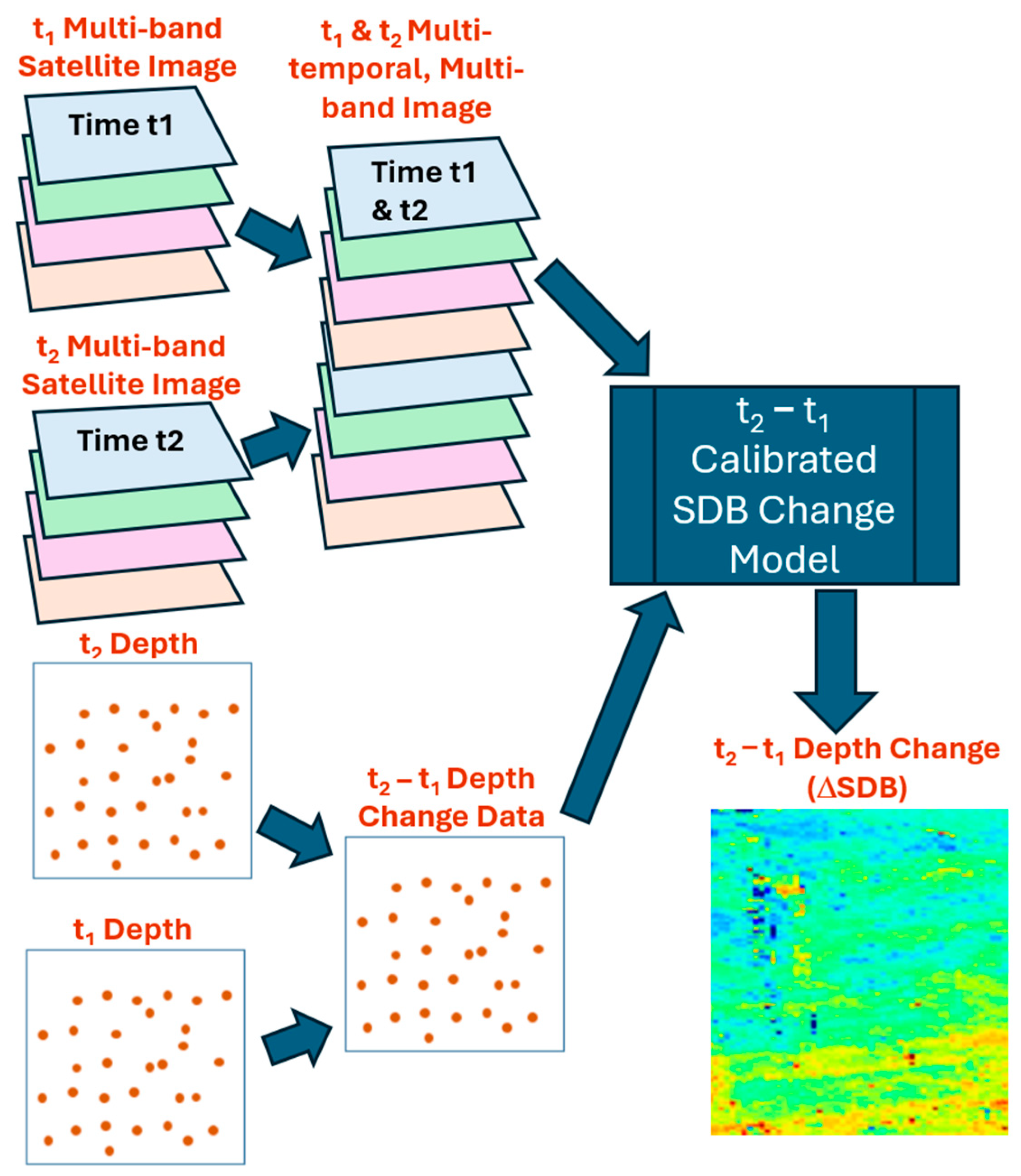
Though intuitive, an alternative approach that has not yet been explored can be formulated. Suppose that in addition to having two images—one each for t1 and t2—one has spatially coincident reference depth data for t1 and t2. In such cases, a single multi-temporal image can be produced by “stacking” the t1 and t2 images, “true” depth change can be calculated for image pixels by differencing the reference data depths, and a single empirical model can be fitted that estimates depth change directly using the multi-temporal “stacked” image. Figure 2 presents a schematic of this alternative. It comprises the following steps:
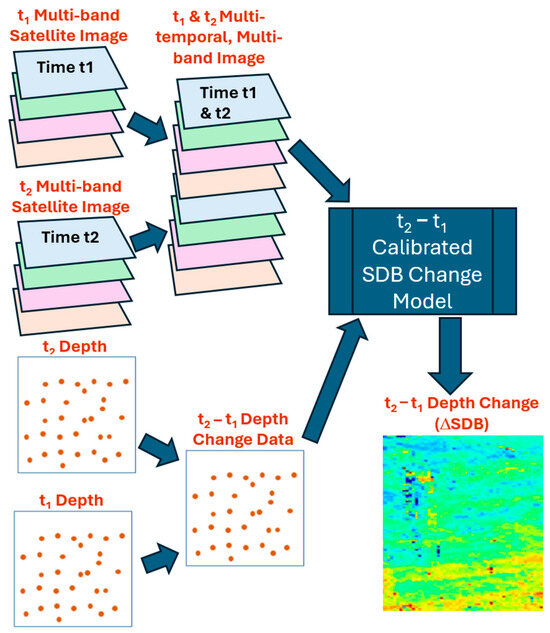
Figure 2.
Schematic of the proposed approach to estimating depth change using SDB.
- Obtain reference depth data and satellite images for two times (t1 and t2).
- Use the reference data to calculate “true” depth change from t1 to t2 for pixels/points for which reference depth data exist for both t1 and t2.
- Combine the images from t1 and t2 into a single multi-temporal “stacked” image.
- Develop a t1 to t2 depth change model using the t1 and t2 band reflectance values of the stacked image and the t1 to t2 depth change reference data.
- Estimate depth change by applying the model to all of the multi-temporal “stacked” t1 + t2 images.
The motivation for exploring and evaluating this alternative for estimating depth change using an empirical SDB depth change approach comprises two potential advantages compared to the conventional “two-model-differencing” approach. First, the conventional approach causes an implicit loss of depth change information. Whereas the conventional approach implicitly treats t1 and t2 reflectance values for individual pixels as independent observations, it is reasonable to suppose that the temporal difference in reflectance values for each pixel contains a useful depth change signal. Second, in the “two-model-differencing” approach, there are two uncertainties—one for each unitemporal SDB model—that are likely to combine to produce a larger depth change error than would a single model that estimates depth change directly.
The exploration of these suppositions and comparison of results from the conventional “two-model-differencing” approach is the subject of this article.
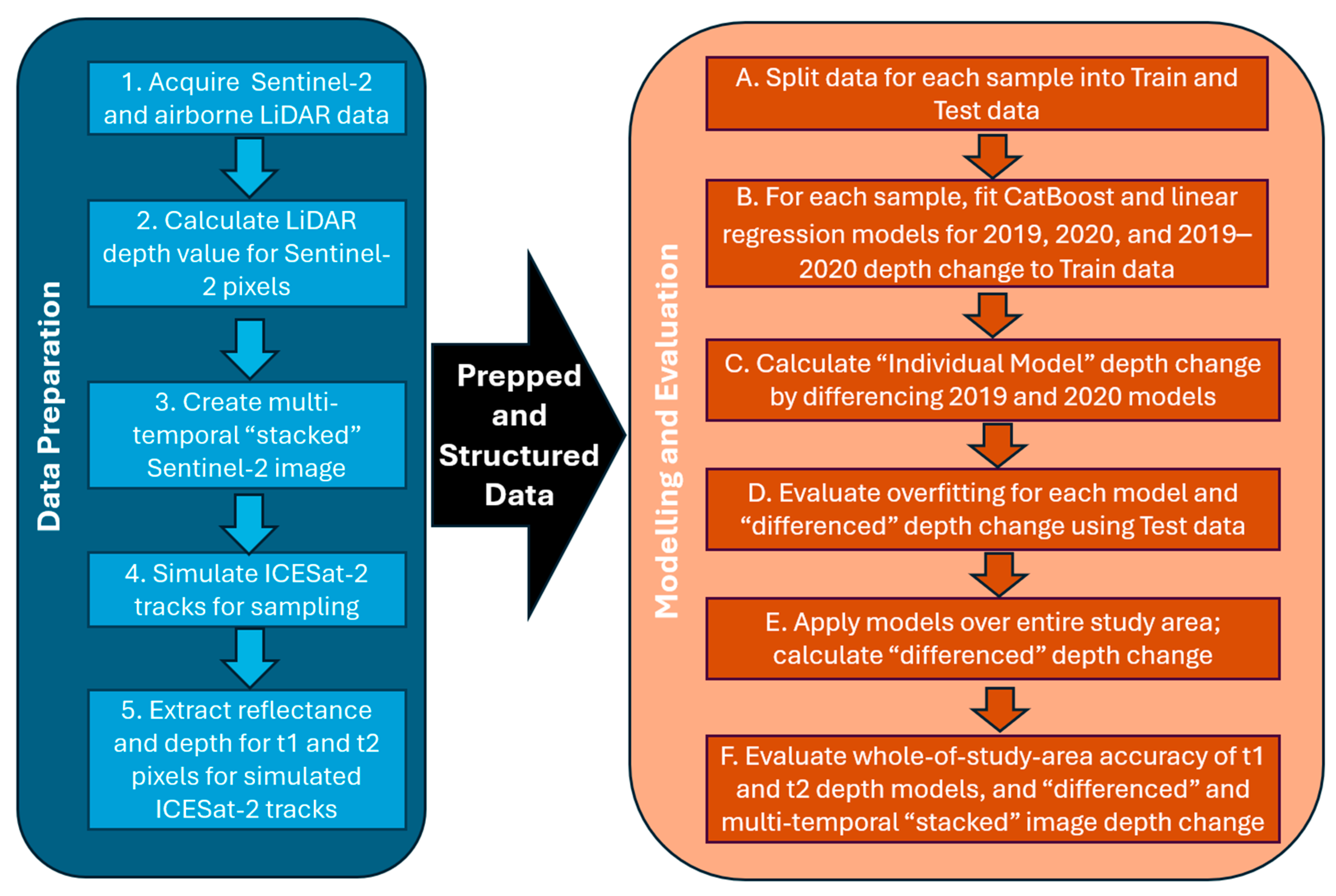
To facilitate an understanding of the data preparation and modelling steps undertaken, a schema showing the general process followed has been included (Figure 3). This is referred to in the text where appropriate.
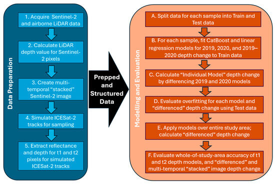
Figure 3.
Data preparation and modelling schema.
2. Materials and Methods
2.1. Study Area and Data
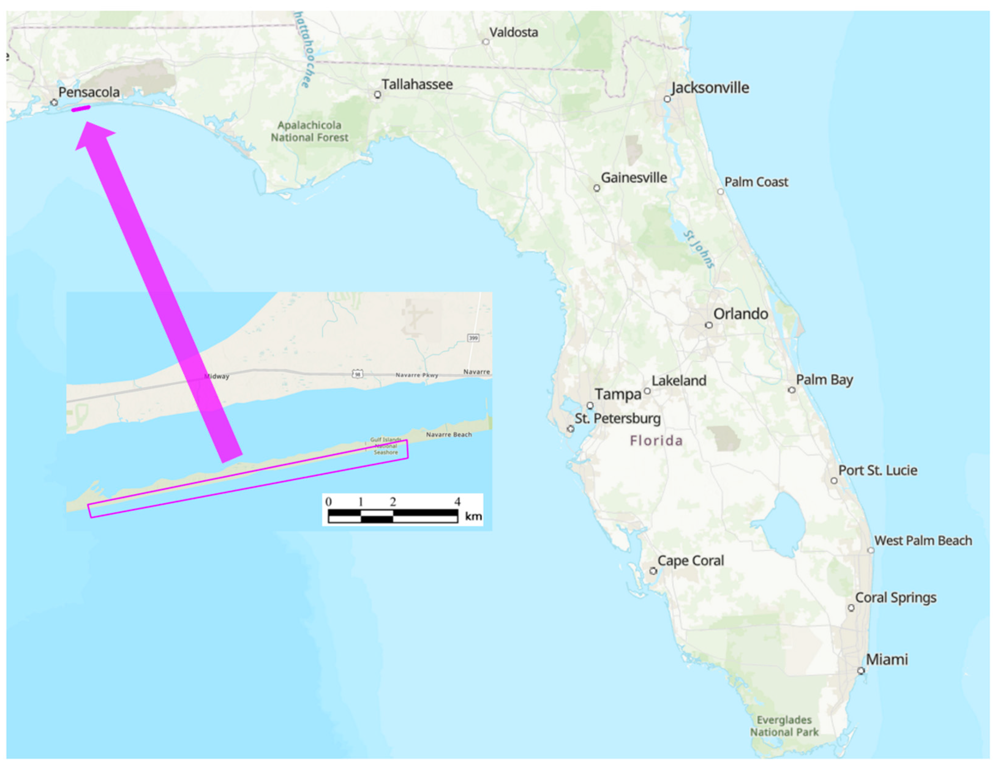
The study area measures approximately 0.5 km (north–south) by 14.5 km (east–west) and is located on Santa Rosa Island, Florida (United States) (Figure 4). This area is on a barrier island for the United States Gulf Coast that was subjected to Category 2 Hurricane Sally on 16 September 2020. The estimation of depth change using Sentinel-2 imagery and ICESat-2 LiDAR data processed through the conventional approach described earlier (Figure 1) is documented in [28]. Data employed herein to explore the multi-temporal “stacked” image depth change approach are the same as those described in that article and below.
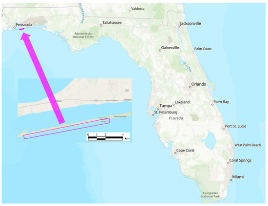
Figure 4.
Study area location (latitude 30.32°/longitude −87.15°).
Pre- and post-hurricane cloud-free Sentinel-2 images were acquired on 21 March 2019 and 19 April 2021, respectively, from the European Space Agency [30] (Box 1, Figure 3). These were atmospherically corrected using ACOLITE [31]. Pre- and post-hurricane airborne LiDAR data were downloaded using the National Oceanographic and Atmospheric Administration’s (NOAA’s) Digital Coast Data Access Viewer [32]. The pre-hurricane reference airborne LiDAR data had been acquired between 27 October 2018 and 20 November 2018 using the green laser (532 nm) of the Teledyne Optech CZMIL (Coastal Zone Mapping and Imaging LiDAR) manufactured by, and sourced from Teledyne Optech (Toronto, ON, Canada). The post-hurricane reference airborne LiDAR data were collected between 22 September 2020 and 13 October 2020 as part of the National Coastal Mapping Program (NCMP) rapid response [33]. Both data sets had been post-processed by the NCMP into digital depth models (DDMs) comprising 1 m pixels using a triangulated irregular network (TIN) approach. For the present work, pre- and post-hurricane depths for each Sentinel-2 pixel were determined by overlaying the 10 m Sentinel-2 pixels on the 1 m DDM and extracting the median DDM value for each Sentinel-2 pixel (Box 2, Figure 3). These values are treated as the reference/“true” depths in this study. Reference/“true” depth change was determined by differencing the values for each pixel with positive values indicating accretion (a decrease in depth) and negative values indicating erosion (an increase in depth) from 2019 to 2020. (Because reference LiDAR data were acquired in 2019 and 2020, the depth change modelled is referred to as “2019 to 2020” despite the reality that the Sentinal-2 images were acquired in 2019 and 2021).
Finally, a multi-temporal image was produced by “stacking” the reflectance values for all 13 Sentinel-2 bands from the pre-hurricane t1 image on the reflectance values of the 13 bands for the post-hurricane t2 image (Box 3, Figure 3). The result was a single 26-band “multi-temporal” t1 and t2 Sentinel-2 image.
2.2. Sampling
The proposed multi-temporal “stacked” image approach to estimating depth change requires spatially coincident data for times t1 and t2. Information about the ICESat-2 satellite and the data it collects was described earlier because its initial orbital path was planned so as to provide such data from repeated coverage of identical overpasses. (Planned ICESat-2 orbits can be downloaded from https://icesat-2.gsfc.nasa.gov/science/specs (accessed on 10 June 2024).) In practice, however, ICESat-2 is pointable, which has often led to non-identical overpasses due to a number of reasons such as the expansion of science priorities and episodic occurrences. Nonetheless, over time, the ICESat-2 data archive will contain spatially coincident multi-temporal data. ICESat-2 was therefore chosen as the “data model” for the present work. Consequently, the complete-coverage airborne LiDAR data were sampled in a manner spatially consistent with ICESat-2 data (Box 4, Figure 3). That is, ICESat-2 overpasses (the term “tracks” is employed herein) were developed using the same data collection characteristics of actual ICESat-2 tracks (Figure 5). For example, because a single ICESat-2 track collects data along three “sub-tracks” spaced 3.2 km apart, this is the spatial pattern by which the airborne LiDAR data were sampled. The simulation algorithm is as follows:

Figure 5.
Example of the sparsest sample employed (“1plus1”—see text) overlain on the “true”/reference bathymetric depth (The number of pixels sampled across all three ICESat-2 tracks is indicated in the legend. The “angles” are the two bearings of actual ICESat-2 overpasses for this area. The study area is located in UTM Zone 17).
First, a single Sentinel-2 pixel was randomly sampled. A “sub-track” that passes through the sample pixel and that has the same orientation (bearing 10.8° N) as one of the two real-world ICESat-2 tracks that cross the area was created, as were two additional parallel sub-tracks spaced 3.2 km apart—one to the east and one to the west of the randomly sampled pixel. These are the purple tracks in Figure 5. The Sentinel-2 pixels along the length of each sub-track were sampled. A second pixel was then randomly sampled, and the process was repeated, except that the second set of sub-tracks had the same orientation as the second real-world ICESat-2 track that crosses the area (bearing 353.0° N). These are the green tracks in Figure 5. Pixels from these six sub-tracks (two tracks) comprised the first sample; this is termed “1plus1” to reflect that there is one track for each of two different bearings. Two additional tracks (each comprising three sub-tracks) with the same orientations were developed and sampled in the same manner and combined with the six sub-tracks from the first two tracks to form a second, denser sample (“2plus2”). Finally, two more tracks were created, and their three sub-tracks were added to the sub-tracks of the first four tracks to form a third, still denser sample (“3plus3”). This increasingly dense sampling was carried out to be able to assess the accuracy of SDB depth change relative to sample density.
Subsequently, all pixels along the sample tracks were extracted for modelling (Box 5, Figure 3).
2.3. Modelling
Recall that the data employed were as follows:
- Two cloud-free atmospherically correct 13-band Sentinel-2 images (10 m spatial resolution) collected prior to, and after, Hurricane Sally, which occurred on 16 September 2020.
- A single multi-temporal Sentinel-2 image created by “stacking” the two Sentinel-2 images.
- Two “true”/reference depth maps derived from airborne LiDAR data collected prior to and after Hurricane Sally.
- Three samples of increasing density of 10 m pixels lying along simulated ICESat-2 sample tracks.
Data structure modifications required for the proposed multi-temporal “stacked” image approach to estimating depth change have been described. However, the proposed method is also likely to require an alternative modelling methodology. In many empirical and quasi-empirical (single-date) SDB studies, modelling methods are employed that implicitly are based on general (quasi-)linear trends in light penetration of water and bottom reflectance for a relatively small number of wavelengths. However, the nature of the predictive relationships among a potentially larger number of wavelengths across two time periods in the proposed “stacked” image approach is unknown. Hence, the proposed approach requires exploration of a suitable machine learning (ML) approach capable of exploiting the predictive structure in the multi-temporal “stacked” image. The ML method employed is described in the following paragraph.
The data from each of the three samples extracted were randomly split into training and testing data sets using an 80/20 split (Box A, Figure 3). Models representing the conventional approach—i.e., individual depth models for t1 and t2—and the proposed method—i.e., a single model to estimate depth change directly using a multi-temporal “stacked” image—of SDB depth change estimation were fitted to the training data set (Box B, Figure 3). This was carried out using linear regression and categorical boosting (“CatBoost;” [34])—a decision-tree-based ML method. Linear regression is commonly used in SDB because it models general trends in data, making it less susceptible to overfitting than many machine learning (ML) methods (including CatBoost). However, this also makes it less likely to be able to identify and employ unknown relationships and interactions in the dependent variables including those that are localized geographically and/or in feature space. Alternatively, because CatBoost models are decision-tree-based models that optimize multiple individual branches of a tree, they have a greater risk of being overfitted, but provide the benefit of being able to find and incorporate “micro-trends” into models.
Initially, all 13 Sentinel-2 spectral bands were considered for modelling. However, preliminary model exploration demonstrated that the bands captured at 60 m resolution—1 (“ultra blue” 443 nm), 9 (short-wave infrared (SWIR) 940 nm), and 10 (SWIR 1375 nm)—contributed little to the models examined. These were eliminated from further analysis. Subsequently, it was considered to discard bands captured at 20 m resolution and only re-sampled to 10 m resolution—5 (very near infrared (VNIR) 705 nm), 6 (VNIR 740 nm), 7 (VNIR, 783 nm), 8 (VNIR 842 nm), 8a (VNIR 865 nm), 11 (short wave infrared (SWIR) 1610 nm), and 12 (SWIR 2190 nm). However, analysis suggested that the use of the visible bands—2 (blue 490 nm), 3 (green 560 nm) 4 (red 665 nm)—combined with bands 6 and 8 would produce the most efficient linear regression and CatBoost models. It was somewhat surprising that bands 6 and 8 clearly contributed something important to models despite being in infrared wavelengths and therefore having little water penetration ability. This will be discussed in the Section 4.
Finally, in addition to reflectance values for bands 2, 3, 4, 6, and 8, commonly used band ratios described by [15,35] were used in modelling. These address the potential non-linear relationship between light reflectance in the blue and red bands (shallowest depths) and blue and green (deeper) depths. These are designated PsBtG (pseudo-bathymetry blue/green ratio) and PsBtR (pseudo-bathymetry blue/red ratio) and are calculated as follows:
where B2(B), B3(G), and B4(R) are reflectance values of, respectively, the blue, green, and red Sentinel-2 bands, and k is an arbitrarily chosen “large” constant that ensures that both logarithms will always be positive. As is usually performed, in this case, k was set equal to 1000.
Out of some 25 band/variable combinations of varying complexity examined, 4 were retained for consideration in modelling. Table 1 summarizes the modelling effort that produced (3 Sample types × 4 Band Combinations × 2 Modelling Fitting Methods × 3 Models for Depth Change =) 72 models.

Table 1.
Summary of variables employed in modelling.
Recall that models were fitted using the training data only. Furthermore, for the individual model approach for depth change, only band and ratio values for 2019 were used in the 2019 models and only band and ratio values for 2020 were used for the 2020 models (Box C, Figure 3). For the single 2019–2020 model fitted to multi-temporal images, band and ratio values for both 2019 and 2020 were employed.
2.4. Model Evaluation
Determining the accuracy of various models and modelling approaches was first performed by examining the goodness-of-fit statistics for each model fitted on the training data, and then comparing depth change model predictions with the “true” airborne LiDAR bathymetric (ALB) values for the training and test data. Model overfitting was evaluated by examining the difference in the goodness-of-fit statistics for the ALB vs. SDB depth change models fitted for the train and test data (Box D, Figure 3). A large difference between the R2 and/or RMSE values for the train and test data sets suggests a given SDB depth change model was overfitted. Particular attention was given to assessing the potential overfitting related to different band combinations and the difference between the two model fitting approaches (CatBoost and logistic regression).
After evaluating overfitting, the models were applied to all pixels in the study area and depth change model predictions were compared to the “true” ALB values statistically and geographically (Boxes E and F, Figure 3).
Finally, the predictive contribution of each variable was assessed globally by calculating a global “importance score”. For CatBoost models, the “importance” of each variable in a model is quantified by the number of decision trees in which a variable appears; this is normalized so that the importance of all variables sums to 100. For linear regression models, importance was measured using the Student’s t value calculated for each variable’s coefficient. (Given that linear regression is a parametric technique, this value can also be tested for statistical significance—unlike the CatBoost importance score.) For each linear regression model, the t values for all variables in a model were normalized to sum to 100 by dividing each t value by the sum of all t values (other than the intercept) and multiplying by 100. For both CatBoost and linear regression models, a global “normalized” importance score for a given variable was obtained by summing its importance in each model and dividing by the number of models in which it appeared. For the multi-temporal “stacked” image depth change models in which a given variable appeared twice—once for 2019 and once for 2020—values were summed to provide a single “normalized” score for the variable.
3. Results
3.1. Overfitting
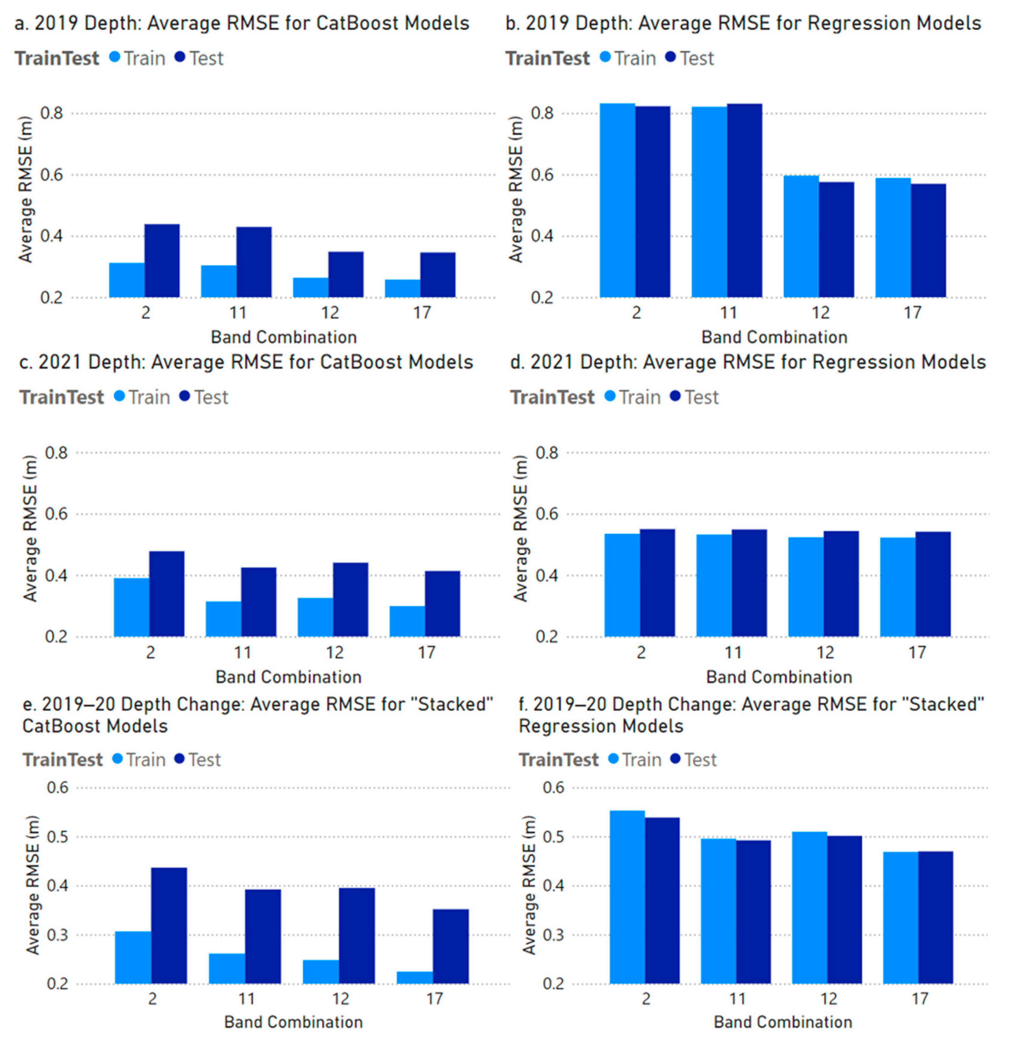
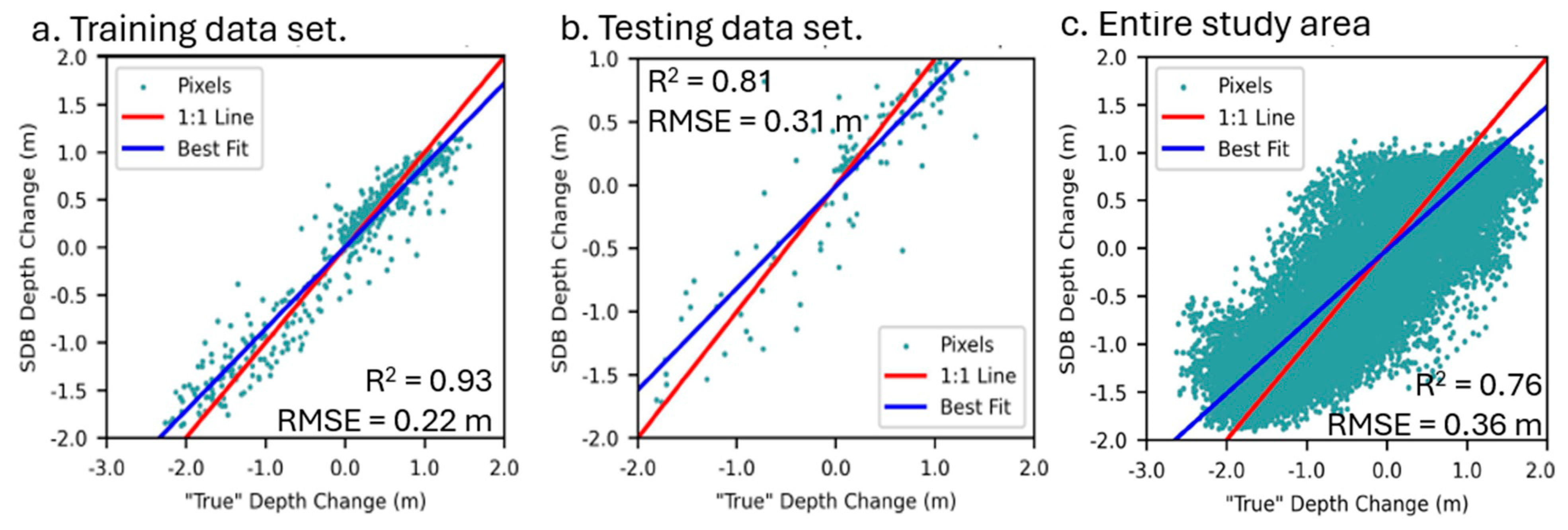
There is evidence of some model overfitting in the CatBoost models for 2019 depth (Figure 6a), 2020 depth (Figure 6c), and the 2019 to 2020 depth change for the multi-temporal “stacked” image (Figure 6e). Figure 7 shows an example scatterplot of the performance of a single multi-temporal “stacked” image depth change model. The average (over all samples) RMSE for CatBoost models fitted on the training data set was approximately 10 cm lower than for the test data set regardless of the band combination. As expected, linear regression models fitted on the training data manifested much less overfitting—i.e., the RMSEs for the train and test data sets were very similar (Figure 6b,d,f). In fact, the linear regression models for 2020 depth performed better for the test data than the train data for all band combinations.

Figure 6.
Average (over all sample types) root mean squared error for residuals for models fitted for train and test data sets. (Band combinations are 2: Visible (2 (blue), 3 (green), 4 (red)); 11: (Visible + 6 (visible and near-infrared (VNIR)) + 8 (VNIR)), 12: (Visible + PsBtG + PsBtR (Equations (1) and (2))); 17 (Visible + VNIR + PsBtG + PsBtR)).

Figure 7.
An example of the performance of one multi-temporal “stacked” image depth change model for the (a) training and (b) testing data sets for one model type (CatBoost in this case), sample type (“3plus3”), and band combination (17), and (c) the model that was fitted applied to the entire data set.
That linear regression produced less overfitted models than the tree-based CatBoost method is not surprising. As noted, tree-based methods provide the benefit of modelling different interactions at different levels and locations of a decision tree, but it is also that capability that makes them susceptible to overfitting. Alternatively, linear regression models general trends, which decreases the likelihood of localized overfitting, but at the potential “cost” in accuracy of ignoring localized tendencies, thereby decreasing global model accuracy. This manifested itself more in the larger RMSEs for linear regression models (Figure 6b,d,f) than in the CatBoost models (Figure 6a,c,e).
Finally, with tree-based ML modelling methods, the risk of overfitting increases as more predictive variables are added to a model. Figure 6a,c,e suggest that this was not a problem with the CatBoost depth change models.
3.2. Depth Change Accuracy
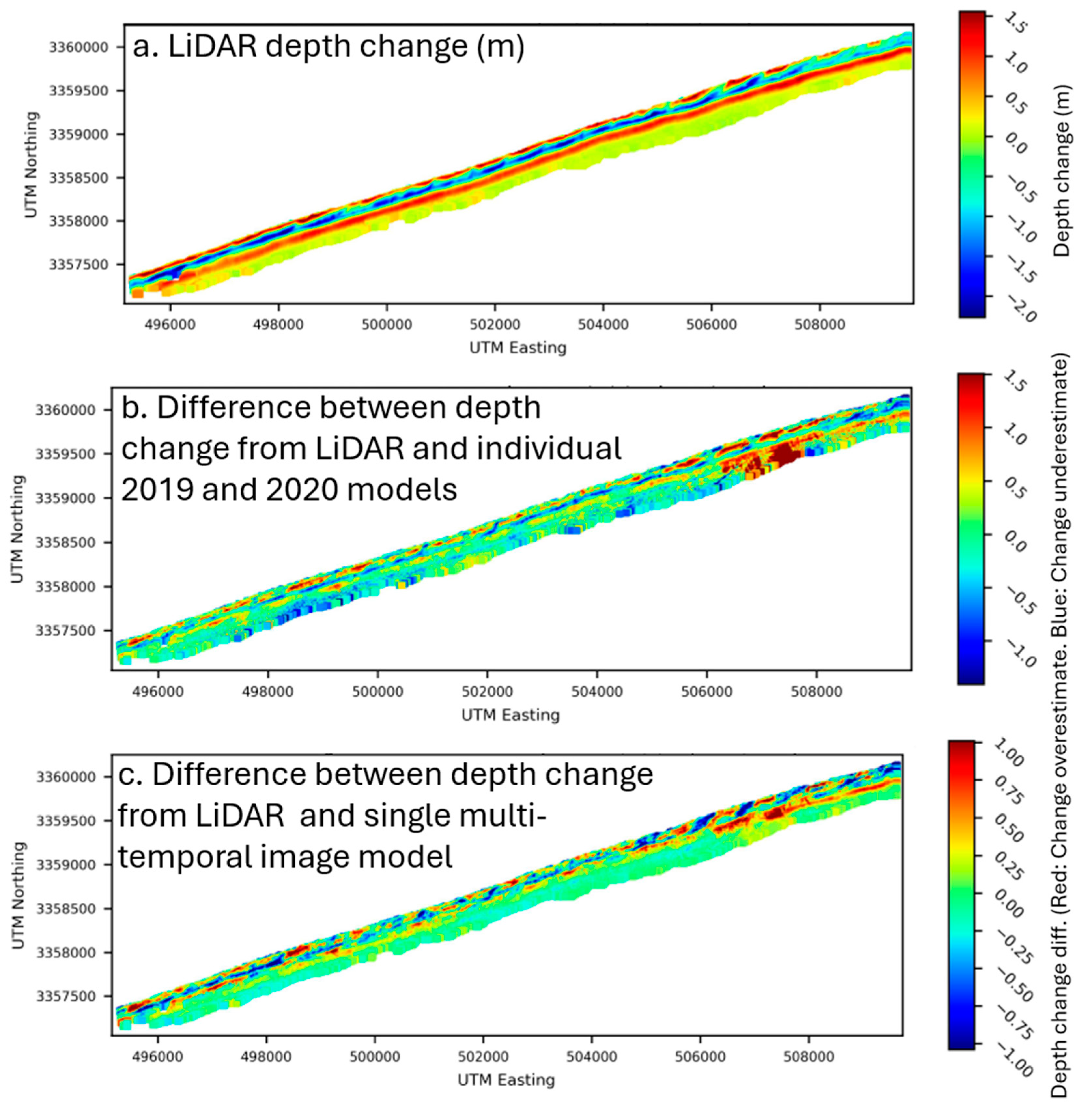
Models were evaluated spatially and statistically and summarized over all 72 models (see Table 1). Figure 8 shows an example of the information examined and used to summarize results over all models. The LiDAR/”true” depth change (Figure 8a) shows consistency from the beach/land on the north edge of the study area to deeper areas in the south with a band of nearshore erosion (blue) and a band of offshore accretion (red). Both models indicate differences for these areas—i.e., deeper red and blue colors for these bands in the difference maps (Figure 8b,c). However, the multi-temporal “stacked” image model (Figure 8c) appears to provide better predictions given the prevalence of its near-zero differences (indicated by the pale-green color). Most notably, the result for the individual model approach Figure 8b shows a (red) block of relatively large depth change overestimation in the northeast that is not present in the multi-temporal “stacked” image model (Figure 8c). This may be an area where water turbidity or image characteristics that were different in 2019 and 2021 were implicitly embedded in the 2019 and/or 2020 models. However, the multi-temporal “stacked” image model (implicitly) ignored whatever anomaly was present.
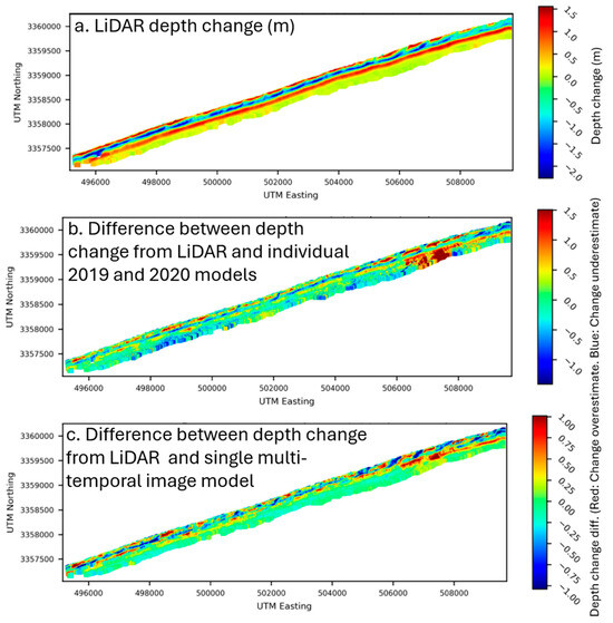
Figure 8.
An example of differences between “true”/LiDAR depth change and CatBoost model-estimated depth change for the entire study area (the study area is located in UTM Zone 17).
Figure 9a,c shows the correlation (R2) between LiDAR/“true” depth change and depth change estimated by fitting individual 2019 and 2020 depth models and differencing the 2019 and 2020 SDB depths, and Figure 9b,d shows the accuracy (RMSE in m) of the estimated depth change.

Figure 9.
Model performance metrics ((a,c): correlation/R2; (b,d): RMSE in m) for estimating depth change using individual SDB models for 2019 and 2021 and differencing the outputs. (Band combinations are 2: Visible (2 (blue), 3 (green), 4 (red)); 11: (Visible + 6 (very near infrared (VNIR)) + 8 (VNIR)), 12: (Visible + PsBtG + PsBtR (Equations (1) and (2))); 17 (Visible + VNIR + PsBtG + PsBtR).
Notable points:
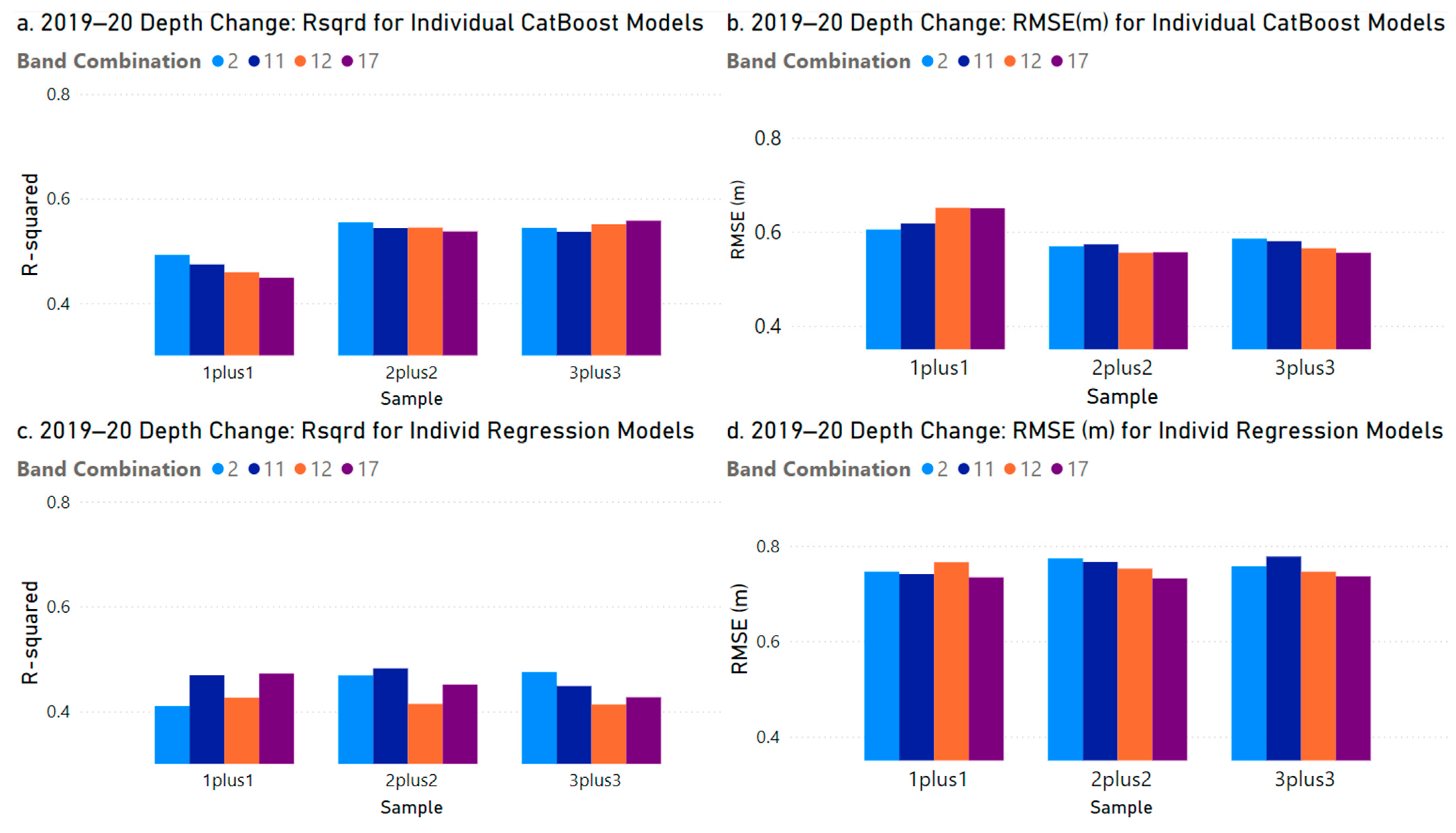
- Doubling the sample size from two tracks (“1plus1”) to four tracks (“2plus2”) produced better CatBoost model difference-based depth change estimates—i.e., R2 values increased (Figure 9a) and RMSE values decreased (Figure 9b). However, a further sample size increase to six tracks (“3plus3”) provided little additional improvement. For linear regression difference models (Figure 9c,d), increasing sample size from two tracks did not improve depth change estimates.
- For CatBoost- and linear regression difference-based models, increased model complexity—i.e., more input variables—improved depth change estimates only slightly (if at all). For example, R2 increased (Figure 9a), and RMSE decreased (Figure 9b) only a small amount from band combination 2 (three variables) to band combination 17 (7 variables).
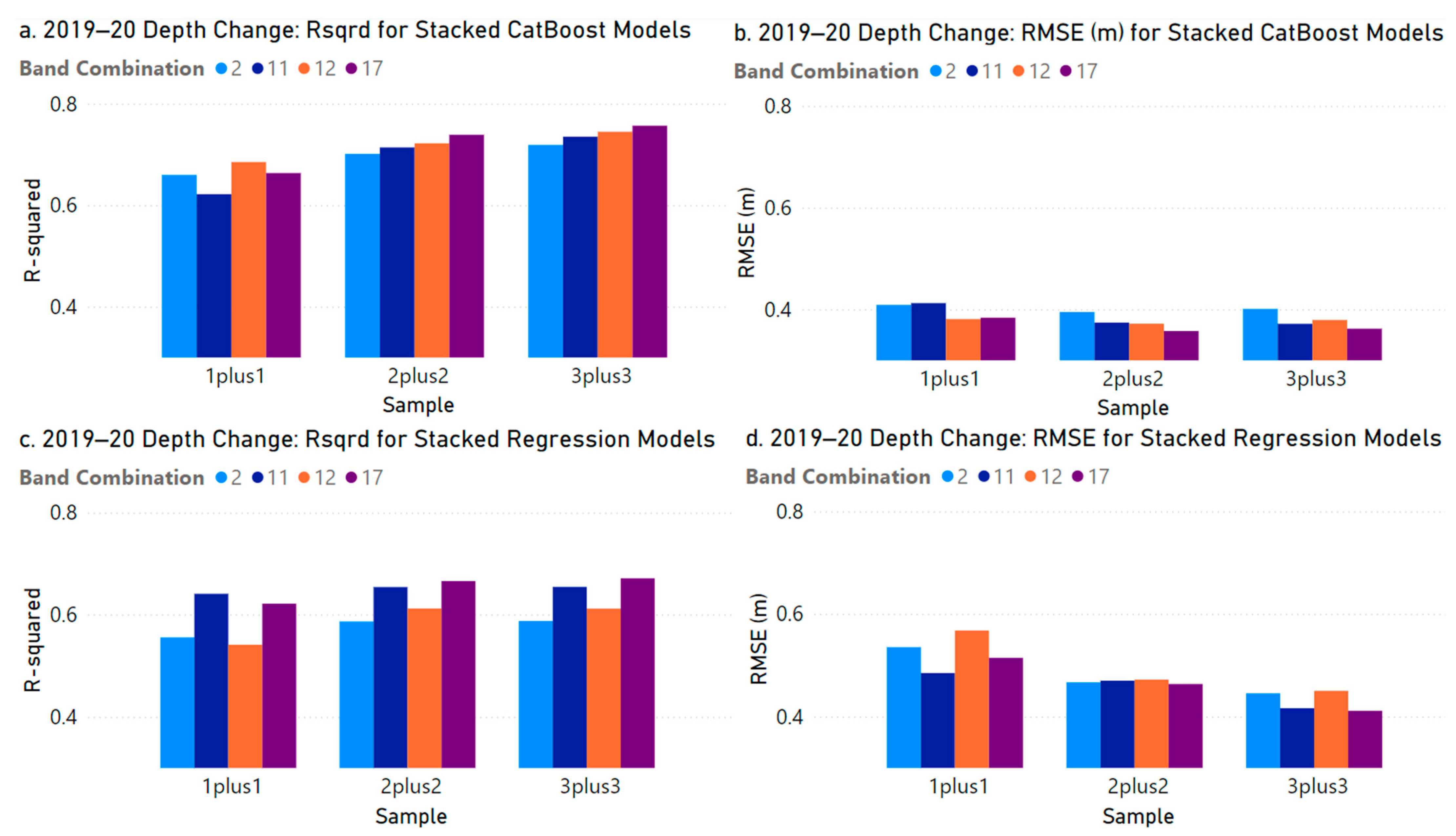
Figure 10a,c shows the correlation (R2) between “true”/LiDAR depth change and depth change estimated by fitting a single depth change model to a multi-temporal “stacked” image area, and Figure 10b,d the accuracy (RMSE in m) of the estimated depth change. The general observations about model performance and depth change accuracy are generally consistent with those noted for the individual model approach (Figure 9):

Figure 10.
Model performance metrics ((a,c): correlation/R2; (b,d): RMSE in m) for estimating depth change using a single depth change model fitted using a multi-temporal “stacked” image. (Band combinations are 2: Visible (2 (blue), 3 (green), 4 (red)); 11: (Visible + 6 (very near-infrared (VNIR)) + 8 (VNIR)), 12: (Visible + PsBtG + PsBtR (Equations (1) and (2))); 17 (Visible + VNIR + PsBtG + PsBtR)).
- Better models result from a sample larger than two tracks, model complexity improves performance, and CatBoost models outperform linear regression models.
Of greatest interest, however, is the focus of this article: the comparative performance of the two modelling approaches to estimating depth change (i.e., the comparison of results in Figure 9 and Figure 10). It is clear that the multi-temporal “stacked” image approach to directly modelling depth change (Figure 10) outperforms the conventional approach of fitting separate t1 and t2 models and differencing their outputs (Figure 9). Across all samples and band combinations, the R2 values for the CatBoost modelling (which performs better than the linear regression modelling) for the multi-temporal “stacked” image approach are about 0.20 higher than for the individual model approach (see Figure 9a vs. Figure 10a). This provides an improvement in accuracy (i.e., a reduction in RMSE) of about 0.15 m (from 0.5m (Figure 9b) to 0.35 (Figure 10b)) or about 30% in an area with an average depth of about 4 m.
Such general statements, of course, are not spatially explicit. However, the spatial distribution of the uncertainty could be assessed by examining information such as was presented in the Figure 8 example; such graphics were produced (but not presented here for article brevity) for all samples, band combinations, and modelling types. In Figure 8, there is an area (red area in the northeast of Figure 8b) of depth change overestimation resulting from the use of CatBoost in the individual model differencing approach while the multi-temporal “stacked” image approach to depth change estimation (Figure 8c) shows no such anomaly. If it were of interest, comparable results for each sample type, band combination, and modelling type could also be examined.
3.3. Variable Importance
Across all models and both model types, the visible bands—blue (B2), green (B3), and red (B4)—had the most predictive power (Figure 11). Moreover, the band ratios comprising the visible bands (PsBTG and PsBtr; see Equations (1) and (2)) also had relatively strong predictive importances. And although the VNIR bands—B6 and B8—had the least importance, analysis indicated that their inclusion clearly increased the R2 correlation values and decreased the RMSE. This was particularly true for the larger and more representative “2plus2” (4 tracks; 12 sub-tracks) and “3plus3” (6 tracks; 18 sub-tracks) samples; this is not apparent in Figure 10 because of averaging across all sample types. Given that infrared light has very limited water penetration ability, it is reasonable to believe that the notable importance of the VNIR bands is related more to their interaction with other bands and seabed morphology than direct effects. That is, VNIR light penetration may be sufficient in shallow areas to interact with the pseudo-bathymetry red ratio (PsBtR), which is known to perform better in shallow areas [35,36].
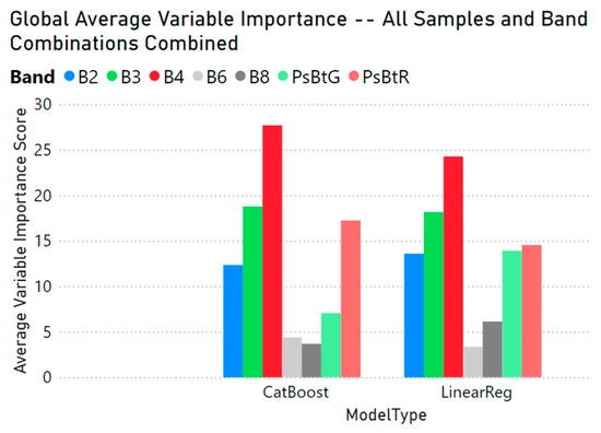
Figure 11.
Average band importance over all samples and band combinations (Bands are B2: Blue; B3: Green; B4: Red; B6: very-near infrared (VNIR); B8: VNIR; PsBtG: pseudo-bathymetry green ratio; ×: PsBtR: pseudo-bathymetry red ratio.).
4. Discussion
A potentially significant limitation to the multi-temporal “stacked” image approach is the need for spatially coincident multi-temporal “true”/reference depth data. A two-model approach (separate models for t1 and t2) does not require this and therefore is more flexible. One potential source of the necessary geographically coincident data was the initial motivation of this work—the ICESat-2 satellite [37]. The orbit of the ICESat-2 satellite is designed to provide repeat LiDAR coverage over identical linear/“widthless” tracks every 91 days. In practice, tracks are not identical, and capture lines are sometimes altered by redirecting the satellite to individual “targets of opportunity”. Nonetheless, the ICESat-2 beam pattern provides coverage of six “sub-tracks”—three sub-tracks 3.2 km apart with each sub-track comprising two “sub-sub_tracks” 90 m apart—that provide broader geographic coverage than a single beam would. Moreover, the use of satellite images with 10 m pixels (e.g., Sentinel-2) relaxes the need for exact geographic coincidence. Another potential source of geographically coincident multi-temporal data is crowd-sourced bathymetric data. However, such data are generally collected from boats and thus may be an unrepresentative sample biased toward areas of navigable depths. Subsequent maps of depth change would be most accurate in deeper areas and least accurate in shallow areas.
There was considerable variation in band importance across models. Figure 11 provides a useful indication of the variables that were generally the most predictive for depth change. However, because Figure 11 presents averages, more specific tendencies that may exist—e.g., interactions between bands and sample sizes—are hidden. Hence, it may be desirable in practice to visually examine graphs and related quantitative information for model fitting and evaluation for train and test data such as is presented in Figure 6. This would potentially avoid the problem of employing an overfitted model that is likely to perform well for the training data set but poorly over an entire area.
The impact of an overfitted model is a decrease in depth change accuracy when a model is applied over an entire area. An example of this is apparent in Figure 7. The model presented is not overfitted—i.e., visually and statistically, its performance for the train (Figure 7a) and test (Figure 7b) data sets does not suggest overfitting. However, its application over the entire study area is much worse (Figure 7c). This outcome can be expected to be even worse if a model is overfitted.
Finally, preliminary work in this study indicated that paramount to predicting depth change accurately is knowledge that depth change occurred in an area. The study area chosen was known to have experienced localized depth change that was sufficiently large to be detected and modelled. (This was assumed to have been episodic/hurricane-related, but it may have been seasonal or long-term erosion.) However, many other candidate areas did not. This was determined to relate to factors such as geomorphology, beach profile, hurricane direction, and local water conditions. Such areas had to be eliminated from analysis to achieve the results presented. Moreover, if a larger area is examined within which areas of depth change are rare/sparse and the magnitude of depth change is relatively small, the depth change signal in the data set will ultimately become too weak to support accurate modelling. In such cases, depth change models will have low goodness-of-fit statistics and estimate that zero (0) depth change—i.e., the mean depth across the area—occurred for all pixels.
5. Conclusions
Using a single multi-temporal “stacked” image and associated depth change “true”/reference data to fit a satellite-derived bathymetry (SDB) depth change model provides superior depth change estimates compared to the more conventional approach of fitting separate SDB models for time t1 and t2 and differencing the result. The former reduced the RMSE from about 50 cm (Figure 9b) to 35 cm (Figure 10b) or 30% in an area with an average depth of about 4 m. Tree-based machine learning (categorical boosting) models outperformed linear regression models. A critical point is that depth change—episodic, seasonal, or long-term—may be so spatially concentrated, which it is difficult to detect and therefore estimate. This suggests that, regardless of the modelling approach employed, there is a need for pre-screening areas to identify those where depth change is likely to have occurred. It also suggests that modelling seasonal depth change that occurs over larger areas may be more amenable to SDB depth change modelling than episodic depth change. This would be a useful avenue for future research.
Author Contributions
Conceptualization K.L.; methodology K.L.; validation K.L.; formal analysis K.L.; investigation K.L.; data curation J.H. and K.L.; writing—original draft preparation K.L.; writing—review and editing K.L. and J.H. All authors have read and agreed to the published version of the manuscript.
Funding
This work was supported by the National Oceanic and Atmospheric Administration (NOAA), grant NA15NOS400020.
Institutional Review Board Statement
Not applicable.
Informed Consent Statement
Not applicable.
Data Availability Statement
All Sentinel-2 data are publicly available free of charge via the European Space Agency’s Copernicus Browser (https://dataspace.copernicus.eu/ (accessed on 10 June 2024)). Users must register on the site before downloading. The relevant image data files have the following prefixes: 2019 data: S2B_MSIL1C_20190321T161949 (not atmospherically corrected) or S2B_MSIL2A_20190321T161949 (atmospherically corrected). 2021 image: S2B_MSIL1C_20210419T161829 (not atmospherically corrected) or S2B_MSIL2A_20210419T161829 (atmospherically corrected). The airborne LiDAR data are available free of charge via NOAA’s data access viewer (https://www.coast.noaa.gov/dataviewer/#/ (accessed on 10 June 2024)) and are named as follows: 2019 LiDAR data: 2019–2020 NOAA NGS Topobathy Lidar DEM: Hurricane Michael (NW Florida). 2020 LiDAR data: 2020 USACE NCMP Post Sally Topobathy Lidar DEM: Gulf Coast (AL, FL, MS).
Acknowledgments
The authors very gratefully acknowledge the contributions of Chris Parrish to this work.
Conflicts of Interest
The authors declare no conflicts of interest.
References
- Kim, M.; Danielson, J.; Storlazzi, C.; Park, S. Physics-based satellite-derived bathymetry (SDB) using Landsat OLI images. Remote Sens. 2024, 16, 843. [Google Scholar] [CrossRef]
- Abbot, R.; Lane, D.; Sinclair, M.; Spruing, T. Lasers chart the waters of Australia’s Great Barrier Reef. Proc. Soc. Photogr. Instrum. Eng. 1996, 2964, 72–90. [Google Scholar]
- Gao, J. Bathymetric mapping by means of remote sensing: Methods, accuracy and limitations. Prog. Phys. Geogr. 2009, 33, 103–116. [Google Scholar] [CrossRef]
- Arsen, A.; Crétaux, J.-F.; Berge-Nguyen, M.; Abarca del Rio, R. Remote sensing-derived bathymetry of Lake Poopó. Remote Sens. 2014, 6, 407–420. [Google Scholar] [CrossRef]
- Forfinski-Sarkozi, N.; Parrish, C. Active-passive spaceborne data fusion for mapping nearshore bathymetry. Photogramm. Eng. Remote Sens. 2019, 85, 281–295. [Google Scholar] [CrossRef]
- Albright, A.; Glennie, C. Nearshore bathymetry from fusion of Sentinel-2 and ICESat-2 observations. IEEE Geosci. Remote Sens. Lett. 2020, 18, 900–904. [Google Scholar] [CrossRef]
- Thomas, N.; Pertiwi, A.; Traganos, D.; Lagomasino, D.; Poursanidis, D.; Moreno, S.; Fatoyinbo, L. Space-borne cloud-native satellite-derived bathymetry (SDB) models using ICESat-2 and Sentienl-2. Geophys. Res. Lett. 2021, 48, e2020GL092170. [Google Scholar] [CrossRef]
- Kutser, T.; Miller, I.; Jupp, D. Mapping coral reef benthic substrates using hyperspectral space-borne images and spectral libraries. Estuar. Coast. Shelf Sci. 2006, 70, 449–460. [Google Scholar] [CrossRef]
- Ma, S.; Tao, Z.; Yang, X.; Yu, Y.; Zhou, X.; Li, Z. Bathymetry retrieval from hyperspectral remote sensing data in optical-shallow water. IEEE Trans. Geosci. Remote Sens. 2014, 52, 1205–1212. [Google Scholar] [CrossRef]
- Le, Y.; Hu, M.; Chen, Y.; Yan, Q.; Zhang, D.; Li, S.; Zhang, X.; Wang, L. Investigating the shallow-water bathymetric capability of Zhuhai-1 spaceborne hyperspectral images based on ICESat-2 data and empirical approaches: A case study in the South China Sea. Remote Sens. 2022, 14, 3406. [Google Scholar] [CrossRef]
- Le Quilleuc, A.; Collin, A.; Jasinski, M.; Devillers, R. Very high-resolution satellite-derived bathymetry and habitat mapping using Pleiades-1 and ICESat-2. Remote Sens. 2022, 14, 133. [Google Scholar] [CrossRef]
- Lee, Z.; Carder, K.; Mobley, C.; Steward, R.; Patch, J. Hyperspectral remote sensing for shallow waters. I. a semi-analytical model. Appl. Opt. 1998, 37, 6329–6338. [Google Scholar] [CrossRef]
- Brando, V.; Anstee, J.M.; Wettle, M.; Dekker, A.; Phinn, S.; Roelfsema, C. A physics-based retrieval and quality assessment of bathymetry from suboptimal hyperspectral data. Remote Sens. Environ. 2009, 113, 755–770. [Google Scholar] [CrossRef]
- O’Neill, N.; Miller, R. On calibration of passive optical bathymetry through depth soundings analysis and treatment of errors resulting from the spatial variation of environmental parameters. Int. J. Remote Sens. 1989, 10, 1481–1501. [Google Scholar] [CrossRef]
- Stumpf, R.; Holderied, K.; Sinclair, M. Determination of water depth with high-resolution satellite imagery over variable bottom types. Limnol. Oceanogr. 2003, 48 Pt 2: Light in Shallow Waters, 547–556. [Google Scholar] [CrossRef]
- Poursanidis, D.; Traganos, D.; Reinartz, P.; Chrysoulakis, N. On the use of Sentinel-2 for coastal habitat mapping and satellite-derived bathymetry estimation using downscaled coastal aerosol band. Int. J. Appl. Earth Obs. Geoinf. 2019, 80, 58–70. [Google Scholar] [CrossRef]
- Sagawa, T.; Yamashita, Y.; Okumura, T.; Yamanokuchi, T. Satellite derived bathymetry using machine learning and multi-temporal satellite images. Remote Sens. 2019, 11, 1155. [Google Scholar] [CrossRef]
- Kibele, J.; Shears, N. Non-parametric empirical depth regression for bathymetric mapping in coastal waters. IEEE J. Sel. Top. Appl. Earth Obs. Remote Sens. 2016, 9, 5130–5138. [Google Scholar] [CrossRef]
- Danilo, C.; Melgani, F. High-coverage satellite-based coastal bathymetry through a fusion of physical and learning methods. Remote Sens. 2019, 11, 376. [Google Scholar] [CrossRef]
- NASA. No Date-b. ICESat-2 Overview. Available online: https://icesat-2.gsfc.nasa.gov/ (accessed on 10 June 2024).
- Magruder, L.; Neumann, T.; Kurtz, N. ICESat-2 early mission synopsis and observatory performance. Earth Space Sci. Res. Lett. 2021, 8, e2020EA001555. [Google Scholar] [CrossRef]
- NASA. No Date-a. ICESat-2 Data Products. Available online: https://icesat-2.gsfc.nasa.gov/science/data-products (accessed on 10 June 2024).
- Kratzmann, M.; Hapke, C. Quantifying anthropogenically driven morphologic changes on a barrier island: Fire Island National Seashore, New York. J. Coast. Res. 2012, 28, 76–88. [Google Scholar] [CrossRef]
- Hartman, M.; Kennedy, A. Depth of closure over large regions using airborne bathymetric lidar. Mar. Geol. 2016, 379, 52–63. [Google Scholar] [CrossRef]
- Pye, K.; Bolt, S. Assessment of beach and dune erosion and accretion using lidar: Impact of the stormy 2013–14 winter and longer-term trends on the Sefton Coast, UK. Geomorphology 2016, 266, 146–167. [Google Scholar] [CrossRef]
- Misra, A.; Ramakrishnan, B. Assessment of coastal geomorphological changes using multi-temporal satellite-derived bathymetry. Cont. Shelf Res. 2020, 207, 104213. [Google Scholar] [CrossRef]
- Caballero, I.; Stumpf, R. On the use of Sentinel-2 satellites and lidar surveys for change detection of shallow bathymetry: The case study of North Carolona inlets. Coast. Eng. 2021, 169, 103936. [Google Scholar] [CrossRef]
- Hermann, J.; Magruder, L.; Markel, J.; Parrish, C. Assessing the ability to quantify bathymetric change over time using solely satellite-based measurements. Remote Sens. 2022, 14, 1232. [Google Scholar] [CrossRef]
- Madore, B. Investigating Nearshore Bathymetric Change over Time Using Satellite Derived Bathymetry and NOAA’s SatBathy Tool. Unpublished. Master’s Thesis, Oregon State University, Corvallis, OR, USA, May 2024; 72p. [Google Scholar]
- ESA (European Space Agency). Sentinel-2 MSI User Guide. Available online: https://sentinels.copernicus.eu/web/sentinel/user-guides/sentinel-2-msi (accessed on 10 June 2024).
- RBINS (Royal Belgian Institute of Natural Sciences). Available online: https://odnature.naturalsciences.be/remsem/software-and-data/acolite (accessed on 10 June 2024).
- NOAA. No Date. Digital Coastal Data Access Viewer. Available online: https://coast.noaa.gov/digitalcoast/data/jalbtcx.html (accessed on 10 June 2024).
- NCMP (National Coastal Mapping Program). Key Word Search/Find: Hurricane Sally. Available online: https://coast.noaa.gov/digitalcoast/data/home.html (accessed on 10 June 2024).
- Prokhorenkova, L.; Gusev, G.; Vorobev, A.; Dorogush, A.; Gulin, A. CatBoost: Unbiased boosting with categorical features. In Proceedings of the 32nd Conference on Neural Information Processing Systems (NeurIPS 2018), Montreal, QC, Canada, 2–8 December 2018; 11p. Available online: https://proceedings.neurips.cc/paper_files/paper/2018/file/14491b756b3a51daac41c24863285549-Paper.pdf (accessed on 12 August 2024).
- Caballero, I.; Stumpf, R. Atmospheric correction for satellite-derived bathymetry in the Caribbean waters: From a single image to multi-temporal approaches using Sentinel-2A/B. Opt. Express 2020, 28, 11742–11766. [Google Scholar] [CrossRef]
- Caballero, I.; Stumpf, R. Towards routine mapping of shallow bathymetry in environments with variable turbidity: Contribution of Sentinel-2A/B satellites mission. Remote Sens. 2020, 12, 451. [Google Scholar] [CrossRef]
- ICESat-2, No Date. “Orbital Path”. Available online: https://icesat-2.gsfc.nasa.gov/fast-facts (accessed on 10 June 2024).


Disclaimer/Publisher’s Note: The statements, opinions and data contained in all publications are solely those of the individual author(s) and contributor(s) and not of MDPI and/or the editor(s). MDPI and/or the editor(s) disclaim responsibility for any injury to people or property resulting from any ideas, methods, instructions or products referred to in the content. |
© 2024 by the authors. Licensee MDPI, Basel, Switzerland. This article is an open access article distributed under the terms and conditions of the Creative Commons Attribution (CC BY) license (https://creativecommons.org/licenses/by/4.0/).