Abstract
Information about estuarine mixing and its control of sediment transport is crucial to elucidating the dynamics and evolution of estuaries. Here, the microtidal and funnel-shaped Zhenhai Estuary, located in the southwestern Pearl River Delta of China, is used to investigate the characteristics and mechanisms of water mixing and sediment transport based on observations from three spring tides. The results reveal that the studied estuary remains well mixed during spring tides from 2013–2022 despite its microtidal regime. Tidal stirring, which is enhanced by tidal energy convergence and benefits from the funnel-shaped geometry and shallow bathymetry, favors vertical mixing, contributing to the formation of strong mixing in the estuary. Due to the well-mixed regime, sediment transport in the estuary is dominated by the advective term, followed by a moderate tidal pumping term and minor estuarine circulation term. Accordingly, sediments within the estuary tend to be transported landward owing to the regulation of the funnel-shaped geometry, and a gradual but slow infilling trend is predictable. This paper deepens our understanding of hydrodynamics and sediment transport in microtidal estuaries.
1. Introduction
The estuary hosts a variety of economic development activities, including port construction, industrial development, tourism, and aquaculture. Estuaries are also important ecosystems globally, containing six billion people by 2025 [1,2]. With the combined actions of tides, waves, and river discharges, the hydrodynamics in estuaries can be extremely complex. Understanding estuarine hydrodynamics and sediment transport is, therefore, essential to the utilization and protection of estuaries.
The stratification and mixing characteristics of an estuary play a crucial role in driving estuarine evolution and represent a major subject of estuarine hydrodynamics research. As shown by Dyer, relative to well-mixed estuaries, density gradients that develop in stratified estuaries resist turbulence-induced momentum exchange, and thus additional velocity shear is required to generate mixing [3]. Numerous studies have been conducted on estuarine stratification and mixing [4,5,6,7,8,9,10,11,12], and these studies have indicated that the relative strength of river discharge and the tidal prism regulates the mixing regime. For example, macrotidal estuaries, with tidal ranges larger than 4 m, are generally well mixed, as observed in Qiantangjiang Estuary; microtidal estuaries, with tidal ranges < 2 m, are typically partially mixed or stratified, such as Lingdingyang Estuary and Huangmaohai Estuary [5]. Estuaries with large water discharge are generally strongly stratified in the wet season, such as Changjiang and Modaomen estuaries. An estuary can exhibit spring–neap shifts in its mixing regime (well mixed or partially mixed during the spring tide and stratified during the neap tide), especially in tide-dominated estuaries with low river flow [13]. However, little information is available related to stratification and mixing in estuaries with both small water discharge and microtidal conditions; whether such estuaries can produce strong mixing remains an open question.
The type of mixing has a significant impact on sediment transport in estuaries [4,6,14]. This impact is particularly significant during spring tides [15,16,17,18]. Strong mixing during spring tides generally destroys the stratification of the water column, reduces two-layered exchange flow, and facilitates seaward sediment transport. The enhanced stratification that arises during ebb tides suppresses bottom turbulence and confines sediment near the bottom, while the enhanced mixing of flood tides reinforces bottom turbulence and enables the entrainment of bottom sediment into the upper water column [19,20,21]. Typically, stronger flood currents during spring tides result in more sediment transport and significant morphological change due to increased energy and water volume; therefore, the hydrodynamics during spring tides are worthy of attention. Despite numerous studies on estuarine hydrodynamic processes, comprehensive discussion of the characteristics and mechanisms of mixing and related sediment transport during spring tides in microtidal estuaries has been rare.
Zhenhai Estuary (ZHE) is a typical microtidal estuary with little riverine water discharge. There is great demand for deepening of the waterway in the estuary due to the rapid economic development of the surrounding estuarine area. Information about the hydrodynamics and sediment transport of this estuary is required for waterway development and resource management. This study aims to analyze (i) the temporal and spatial variations of mixing during the spring tide, (ii) identify the major factors that affect mixing in ZHE, and (iii) investigate suspended sediment transport characteristics under various conditions. This study can particularly deepen our understanding of the hydrodynamics and sediment transport during spring tide in the microtidal estuary.
2. Study Area
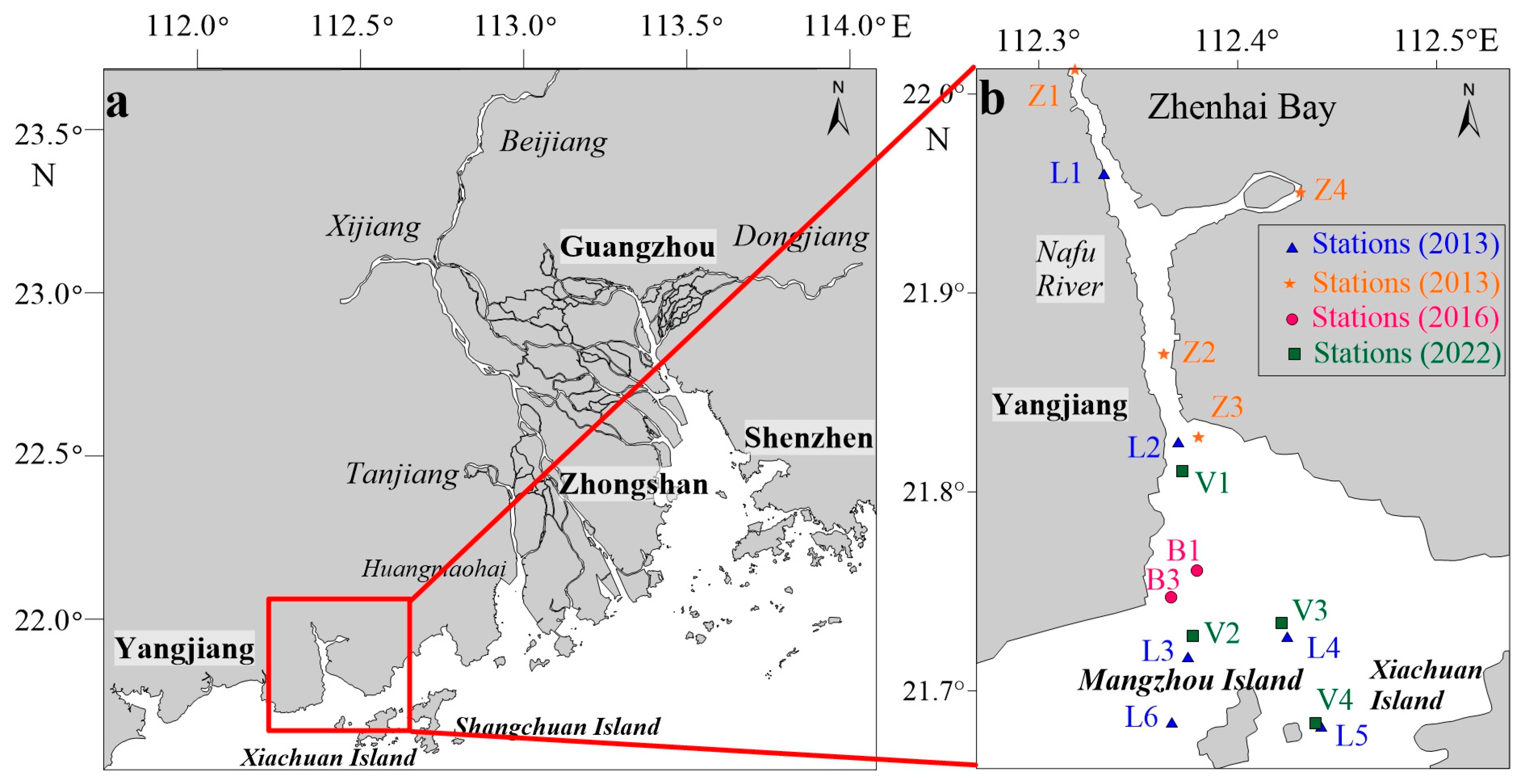
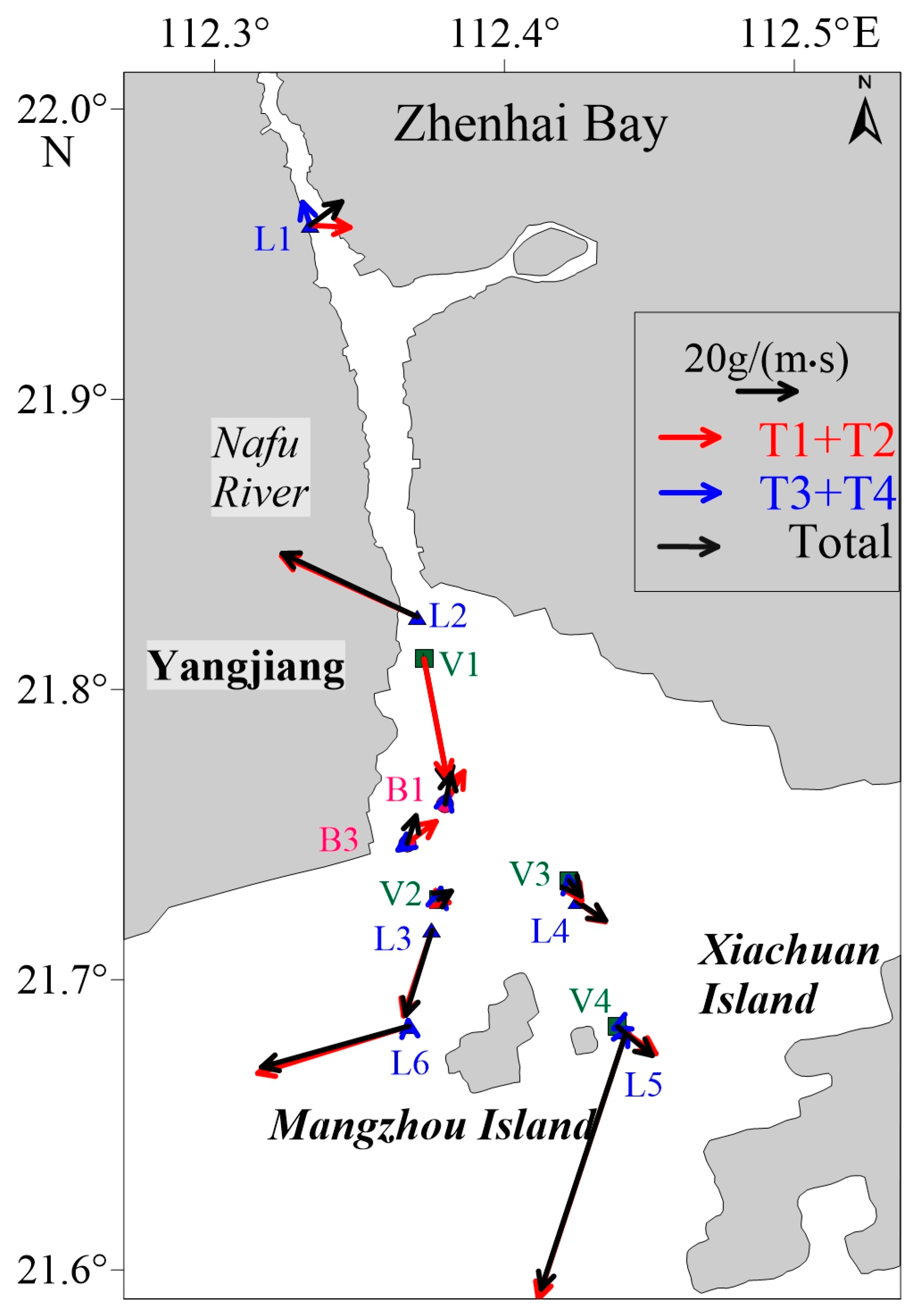
ZHE is located southwest of the Pearl River Estuary and has a drowned valley morphology with a distinct funnel shape (Figure 1). ZHE has a width of around 2500 m at the outlet from east to west. This estuary receives small amounts of water inflow from the upstream Nafu River. Notably, to the south of the outlet lies a deep channel that stretches for approximately 9 km. This deep channel plays a pivotal role as the main channel for tidal currents and has water depths of 4–8 m. Shallow shoals are present on the east and west sides of the estuary, with water depths ranging from −0.5 to 1 m (Figure 1). The estuary is predominantly composed of fine sandy clay. The outlet of the estuary is protected by the Mangzhou, Shangchuan, and Xiachuan Islands, which act as natural barriers. Therefore, the influence of waves on the estuary is relatively small. The upstream Nafu River has a relatively low average annual discharge, with a mean discharge of <100 m3/s. Consequently, ZHE is primarily influenced by tidal action, driven by an irregular semidiurnal tide with a tidal range of 1–2 m. ZHE is located in the subtropical marine climate zone and is influenced by the East Asian monsoon. During summer, the prevailing winds are predominantly southerly, while during the winter months, northerly winds are dominant.
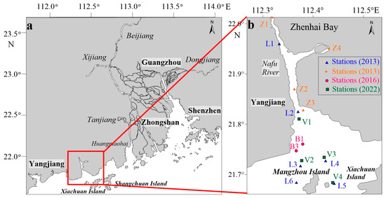
Figure 1.
Location of the Zhenhai Estuary in relation to the Pearl River Delta (a) and measurement stations on 12–13 March 2013, 7–10 May 2016, and 12–13 August 2022 (b).
3. Materials and Methods
3.1. Field Measurement
There have been several short-term field measurements conducted in the estuary in recent years. To cover the wide hydrological conditions as much as possible, all the available data were collected for analysis in this study. The data sets during the spring tides include 12–13 March 2013, 7–10 May 2016, and 12–13 August 2022. Meanwhile, the data sets also include 1–31 March 2013. The instrumentation and observation period are summarized in Table 1. The locations of the measurement stations are shown in Figure 1.

Table 1.
Instruments for measurement.
The field work in March 2013 was conducted by the Research Institute of estuary and coast of Sun Yat-sen University, and funded by the Guangdong provincial waterway bureau in order to develop the navigation channel in the ZHE. The field work consisted of 6 fixed stations (L1–L6) along the deep channel and possible route of the navigation waterway, aiming to measure the current, salinity, and suspended sediment concentration profiles for a 25 h duration (12–13 March 2013) at hourly intervals (Figure 1b). The field work consisted of 4 fixed stations (Z1–Z4), aiming to measure the tidal level for a month duration at hourly intervals (1–31 March 2013). The tidal level were measured by pressure-type sensor level meter MPM4700.The currents were measured by Acoustic Doppler current profiler (ADP). Water temperature and salinity was measured by Optical backscatter (OBS). The suspended sediment concentrations were obtained by collecting water samples and filtering, drying, and weighing in the laboratory. Salinity were obtained by collecting water samples and being titrated with Silver nitrate in the laboratory. For each cast with total water depth (H) > 5 m, six levels (surface,0.2 H, 0.4 H, 0.6 H, 0.8 H, and bottom) were partitioned in the vertical, while three levels (surface, middle, and bottom) were used for stations shallower than 5 m. Hourly wind speed and direction were measured at stations L2 and L6 using an anemometer. The wind speed was averaged over a 1 min period.
The field work on 7–10 May 2016 was conducted by the Research Institute of Estuary and Coast at Sun Yat-sen University and funded by the local government in order to build the port on the west coast of the ZHE. The field work consisted of two stations located on the western shoal near the possible location of the port (Figure 1b). Each station was occupied for 73 h, and the current, salinity, and sediment concentration profiles were measured at hourly intervals using ADP and OBS. The vertical profiles comprised only three levels (surface, middle, and bottom). Wind data were observed at stations B3 using an anemometer in 10 min intervals.
The field work on 12–13 August 2022 was conducted by Guangdong Yunan Inspection Technology Co. and funded by the Department of Natural Resource of Guangdong Province for the environmental evaluation of the ZHE. The field work consisted of four stations (V1–V4) along the deep channel for 25 h (Figure 1b). The currents were measured by acrylic current meters, and the salinity was measured by a HWYDA-1 laboratory salinometer. The vertical profiles comprised only three levels (surface, middle, and bottom). In the meantime, water samples were collected and then analyzed for the suspended sediment concentration in the laboratory. Wind data were measured using a FYF-1 lightweight anemometer.
3.2. Data Analysis
3.2.1. Analysis of Mixing Type and Dominant Flow
The mixing condition of an estuary can be analyzed using the stratification coefficient N, which is calculated with the following equation:
where ∆s represents the salinity difference between the surface and bottom layers, and s0 refers to the average salinity of the profile. A value of N < 0.15 corresponds to a fully mixed estuary, 0.15 ≤ N ≤ 0.32 corresponds to a partially mixed estuary, and N > 0.32 corresponds to a highly stratified estuary [22].
The equation for calculating the dominant flow is
where E is the area of the ebb tide velocity duration curve and time axis, and F is the area of the flood tide velocity duration curve and time axis. If p > 50%, ebb tidal flow is dominant, while flood tidal flow is dominant at p < 50%. p = 50% indicates an equal volume of ebb and flood tidal flows.
3.2.2. One-Dimensional Potential Energy Anomaly Equation
The potential energy anomaly (ϕ) is very useful in scaling the development and breakdown of mixing and stratification [23]. Based on the classical one-dimensional potential energy anomaly equation proposed by Simpson, the formation and decay of water column stratification in an estuary can be quantitatively analyzed [23,24,25]. This equation decomposes the time derivative of the potential energy anomaly (ϕ) into four components (tidal straining, estuarine circulation, tidal stirring, and wind stirring) and calculates each component separately. Tidal straining can increase stratification during the ebb tide but enhance vertical mixing during the flood tide. Estuarine circulation refers to the longitudinal density gradient driven shear flow, which permanently contributes to stratification, while tidal stirring and wind stirring perpetually enhance vertical mixing.
where ρ is the density profile through the water column of depth h and is the depth-averaged value. The potential energy anomaly (ϕ) is the work that required bringing about complete mixing. ϕ < 20 J/m3 indicates a vertically mixed region [26].
where h is the water depth, = 0.0038 and = 0.039 are the mixing efficiencies, and and are the effective drag coefficients for the bottom and surface stresses, respectively, with = 0.0025 and = 0.000064 [23]. is the density of the bottom-layer water, is the depth-averaged flow velocity in the main direction, and is the depth-uniform horizontal density gradient; its integral is taken over the water column depth h. u and refer to the vertical velocity profile and the vertical average velocity at each moment, respectively, and g is the acceleration due to gravity, is the eddy viscosity, is the total Richardson number, = 1.2 kg/m3 is the density of air, and W represents the wind speed.
3.2.3. Sediment Transport Decomposition Method
Based on the single-width longitudinal sediment transport model [27,28,29], the method can be decomposed as follows:
where u = u(z, t) and c = c(z, t) are the current velocity and SSC (suspended sediment concentration) at the depth, respectively. Moreover, ‘< >’ denotes a tidal-averaged value; ‘-’ denotes a depth-averaged value, ‘t’ denotes a deviation in a tidal cycle, and ‘0’ denotes an average in a tidal cycle. At any depth, and , where and are the deviations of the observed values from the depth-averaged values. The tidal fluctuations are written as and , where and are the deviations from the depth-averaged values in a tidal cycle. Meanwhile, the tidal height is , where is the deviation of the tidal height from the mean depth. In this equation, T1 represents the Eulerian residual transport term, T2 represents the Stokes drift transport term, and T1 + T2 corresponds to the advective transport term. T3 represents the tidal variation associated with SSC, T4 represents the tidal flow variation associated with SSC, and T3 + T4 accounts for the tidal pumping effect. T5 represents terms related to the variations of vertical velocity and SSC. T6 and T7 are terms resulting from the non-uniform vertical distribution of SSC and the non-uniform vertical distribution of flow velocity, respectively. T8 represents vertical shear-induced tidal oscillations. T6 + T7 + T8 collectively constitute the shear dispersion term.
4. Results
4.1. Intratidal Variations of Current, Salinity, and SSC
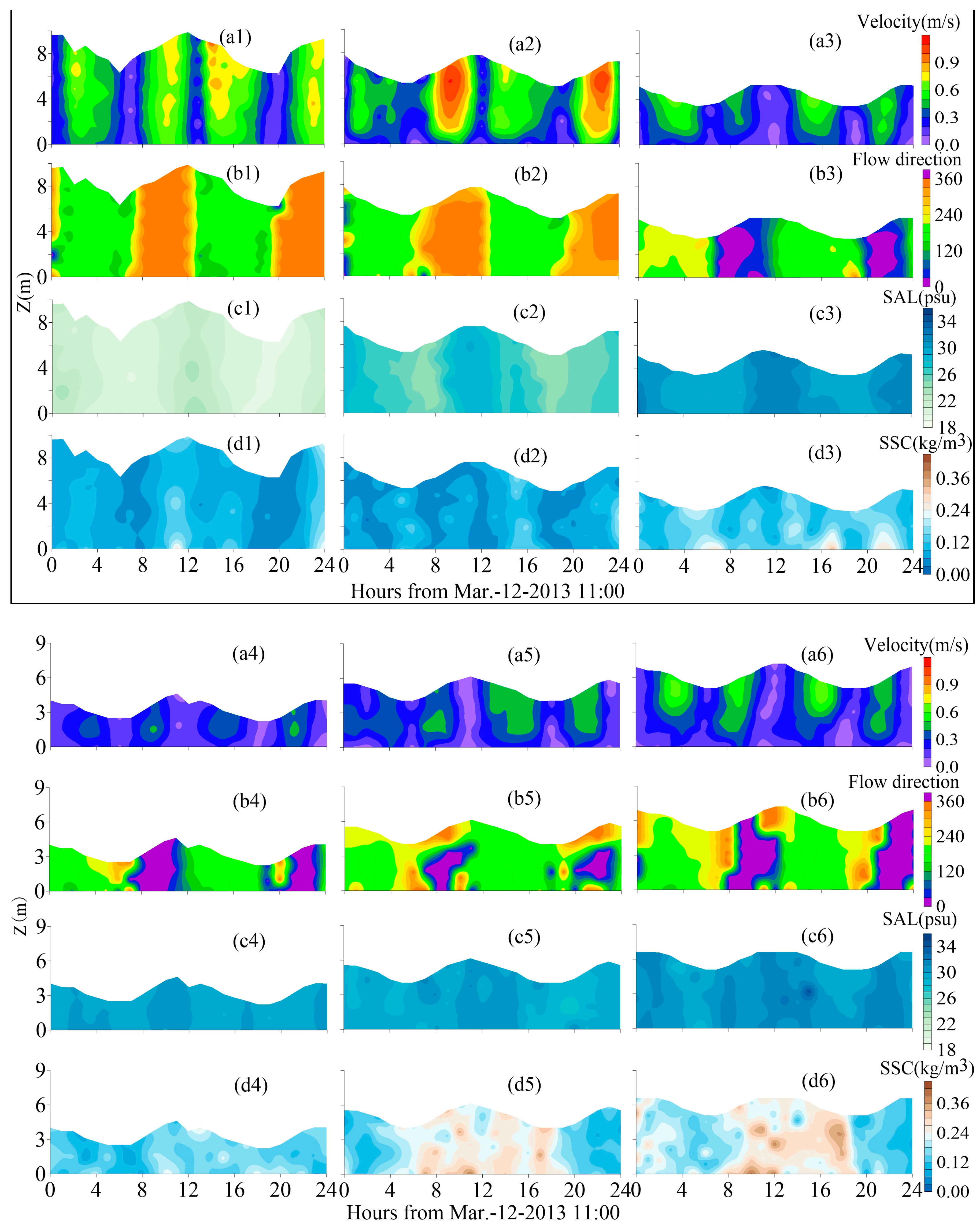
The time series of flow velocity, flow direction, salinity, and SSC at observation stations during 12–13 March 2013, 7–10 May 2016, and 12–13 August 2022 are depicted in Figure 2, Figure 3 and Figure 4. Table 2 provides information about flood and ebb flow velocities, duration, average water depth, SSC, and dominant flow in ZHE.
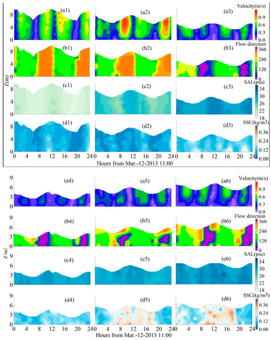
Figure 2.
Time series of flow velocity, flow direction, salinity, and sediment concentrations at L1 (a1,b1,c1,d1), L2 (a2,b2,c2,d2), L3 (a3,b3,c3,d3), L4 (a4,b4,c4,d4), L5 (a5,b5,c5,d5), and L6 (a6,b6,c6,d6).
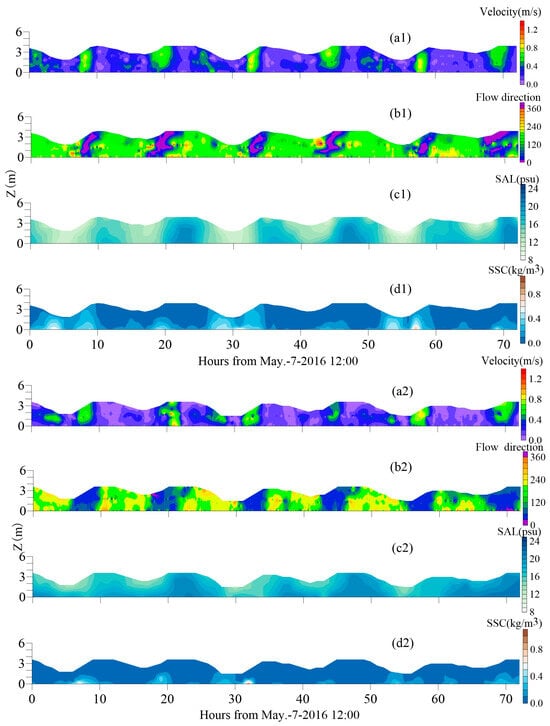
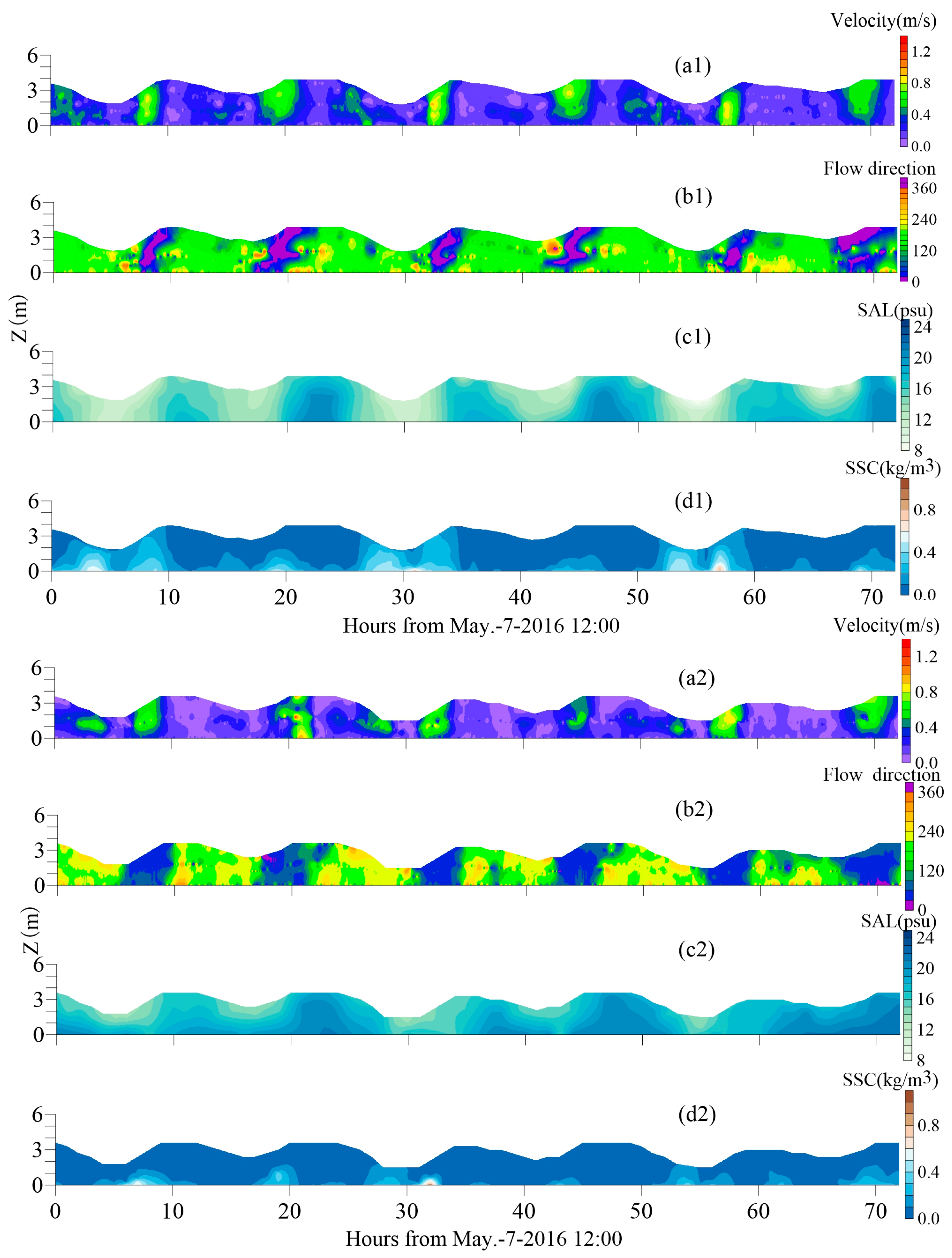
Figure 3.
Time series of flow velocity, flow direction, salinity, and sediment concentrations at B1 (a1,b1,c1,d1) and B3 (a2,b2,c2,d2).
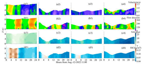
Figure 4.
Time series of flow velocity, flow direction, salinity, and sediment concentrations at V1 (a1,b1,c1,d1), V2 (a2,b2,c2,d2), V3 (a3,b3,c3,d3), and V4 (a4,b4,c4,d4).
Table 2.
Flood and ebb flow velocities, duration, average water depth, SSC, and dominant flow in ZHE.
Longitudinally, the average flow velocity during flood tide gradually increases from the sea toward the outlet due to the convergence effect caused by the trumpet-shaped topography, peaking at the outlet and gradually decreasing landward. Laterally, both the flood and ebb tide average flow velocities are greater at stations on the western side of the estuary than at stations on the eastern side in similar latitudes. During 12–13 March 2013, the maximum measured flood flow velocity of 1 m/s occurred at the surface layer of station L2, while the maximum measured ebb flow velocity was observed in the surface layer of station L1 (1.04 m/s). Station L2 exhibits flood dominance with a dominant flow value of 0.36, while the other five stations exhibit ebb dominance. During 12–13 August 2022, the maximum measured flow velocity during the flood tide occurred in the middle layer of station V1 (1.05 m/s), while the maximum during ebb flow occurred in the surface layer of station V1 (1.09 m/s). Station V2 exhibits flood dominance with a dominant flow value of 0.48, while the other stations show ebb dominance. The patterns of lateral and longitudinal flow velocities align with the observations from March 2013. Stations B1 and B3, situated on the western shoals of ZHE, provide valuable insights into the hydrodynamics and suspended sediment characteristics of shoal areas. During 7–10 May 2016, both stations have dominant flood tides with dominant flow values below 0.5. The maximum flow velocity during flood tide is observed in the middle layer of station B3 (1.30 m/s), while the maximum flow velocity during ebb tide occurs in the middle layer of station B1 (0.79 m/s).
Longitudinally, the average salinity gradually increases from land to sea throughout the tidal cycle. For instance, it rises from 20.68 PSU (L1) to 29.75 PSU (L6). The relatively high salinity observed at station L1, which is located in the river channel, indicates that upstream runoff is relatively small and L1 is strongly affected by tides. Laterally, stations on the western side exhibited greater salinity than those on the eastern side, which have similar latitudes, aligning with the conclusions drawn from the analysis of flow velocity. The average salinities throughout the tidal cycle at stations B1 and B3 are 15.44 and 17.42 PSU. The average salinities throughout the tidal cycle at stations V1–V4 are 11.07, 18.28, 17.59, and 22.00 PSU, respectively. The stratification coefficients of each station are <0.15 among the three observations, indicating a well-mixed estuary.
Laterally, the vertical averages of SSC at stations that have similar latitudes are nearly equal. Longitudinally, the average SSC gradually decreases from the sea to the outlet, reaching its minimum at the outlet and slightly increasing landward during 12–13 March 2013. Meanwhile, the average SSC gradually increases from the sea to the outlet, reaching its maximum at the outlet on 12–13 August 2022. At stations L1–L4, high SSCs occur around the periods of peak flood and ebb flows, indicating a correlation between SSC and tidal variations. The vertical distributions of SSC at stations L1, L2, and L4 are relatively uniform, with maximum values of 0.27, 0.19, and 0.23 kg/m3, respectively. At station L3, SSC is higher near the bottom and diffuses toward the upper layers, with a maximum value of 0.33 kg/m3. At stations L5 and L6, the highest SSC values are generally observed in the middle and near-bottom layers, with a maximum of 0.40 kg/m3. Measured SSCs at stations V1–V4 are relatively small. The maximum SSC is 0.15 kg/m3 at station V1. The vertical variation of SSC is not significant, with slightly higher values in the bottom layer compared to the surface layer. The average SSC is higher at station B1 than at station B3. At station B1, SSC increases only near the bottom and appears during the periods of peak flood and ebb flows, with a high SSC value of 0.81 kg/m3. At station B3, the vertical distribution of SSC is relatively uniform, with bottom-layer SSC reaching 0.96 kg/m3 during the peak flood stage. SSC varies significantly among layers, with higher values in the bottom layer compared to the surface layer.
Wind speeds are relatively low at stations L2 and L6 during 12–13 March 2013, ranging from 0.5 to 4.0 m/s and 2.5 to 7.0 m/s, respectively. The wind speed at stations B1 and B3 ranges from 0.4 to 9.1 m/s, and the wind is predominantly from the south during 7–10 May 2016. Wind speeds at stations V1 and V3 range from 1.7 to 3.3 m/s and 1.8 to 3.5 m/s during 12–13 August 2022, respectively, with an average value of 2.4 m/s. The prevailing wind direction is from the east.
4.2. Attribution of Mixing
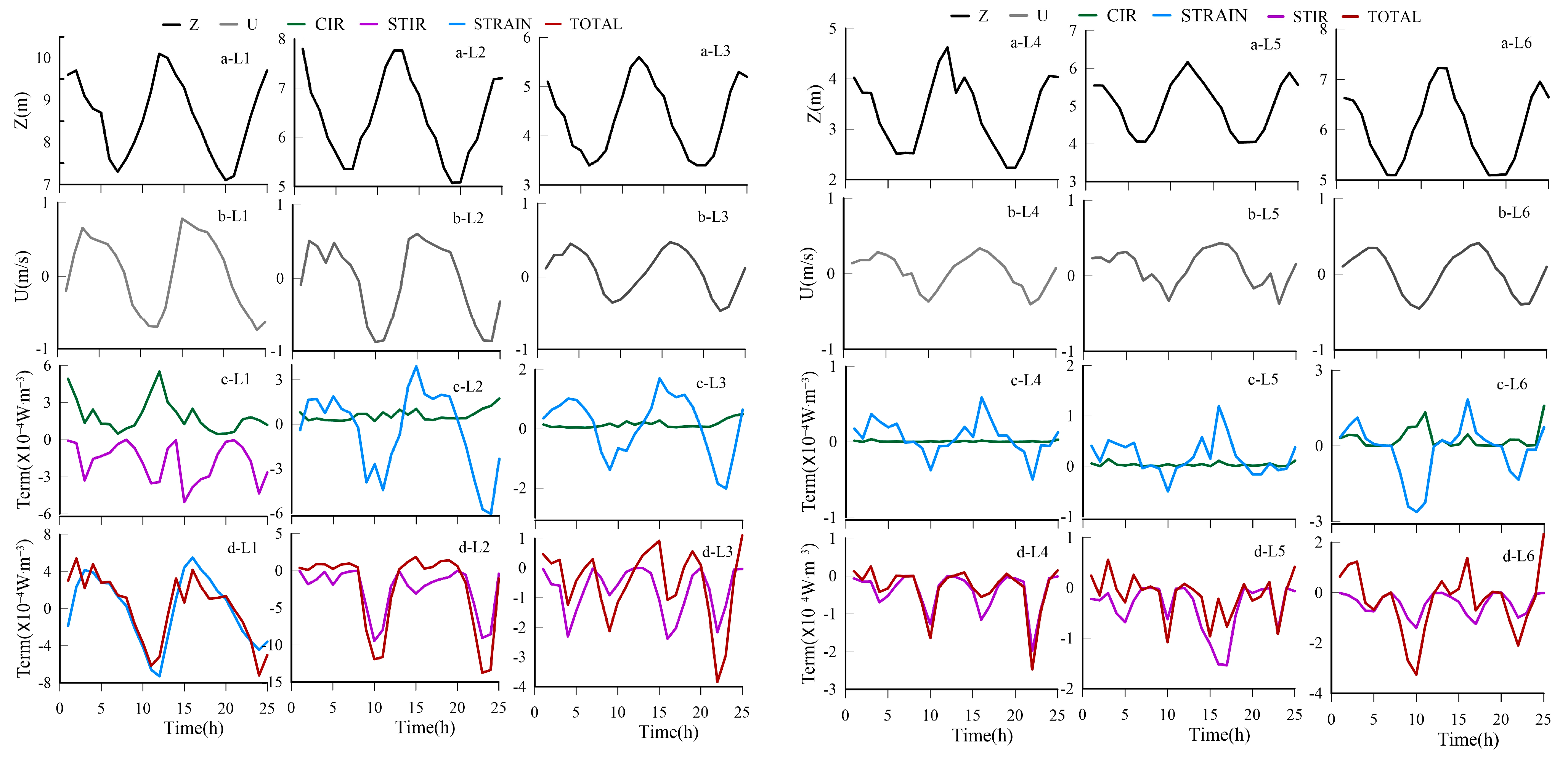
To analyze the dominant mechanisms of different mixing processes, the time series of the water depth, depth-averaged velocity, time derivative of the potential energy anomaly (ϕ) due to tidal straining (∂φ/∂t)strain, estuarine circulation (∂φ/∂t)cir, tidal stirring (∂φ/∂t)stir, and wind stirring (∂φ/∂t)wind at observation stations L1–L6, B1, B3, and V1–V4 during the periods 12–13 March 2013, 7–8 May 2016, and 12–13 August 2022 are depicted in Figure 5, Figure 6 and Figure 7. The tidal means of (∂φ/∂t)strain, (∂φ/∂t)cir, (∂φ/∂t)stir, and (∂φ/∂t)wind at stations L1–L6, B1, B3, and V1–V4 are shown in Table 3.
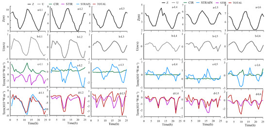
Figure 5.
The water depth, depth-averaged velocity, (∂φ/∂t)strain, (∂φ/∂t)cir, (∂φ/∂t)stir, and (∂φ/∂t)total at L1–L6.
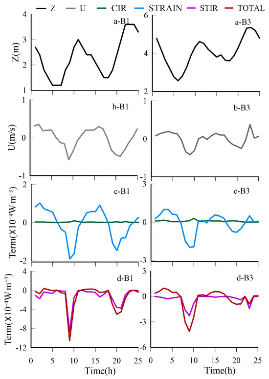
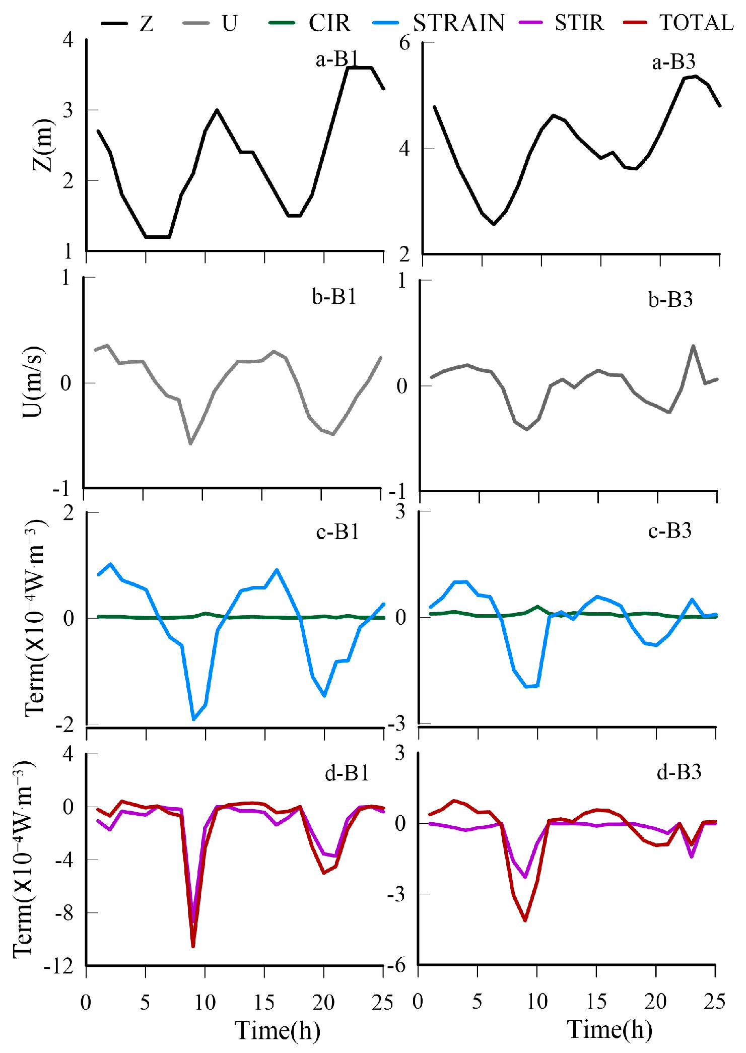
Figure 6.
The water depth, depth-averaged velocity, (∂φ/∂t)strain, (∂φ/∂t)cir, (∂φ/∂t)stir, and (∂φ/∂t)total at B1 and B3.
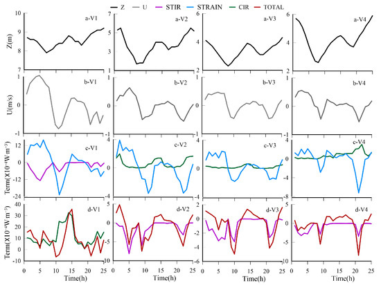
Figure 7.
The water depth, depth-averaged velocity, (∂φ/∂t)strain, (∂φ/∂t)cir, (∂φ/∂t)stir, and (∂φ/∂t)total at V1–V4.
Table 3.
The mean value of (∂φ/∂t)strain, (∂φ/∂t)cir, (∂φ/∂t)stir, and (∂φ/∂t)wind at stations L1–L6, B1, B3, and V1–V4. (unit: ×10−4 W·m−3).
The tidal mean values of ϕ at all observation stations < 20 J/m3, indicating that the mixing condition of each station is vertically mixed, aligning with the conclusions of the stratification coefficient [26]. During 12–13 March 2013, ϕ ranged from 0 to 11.9 J/m3 at stations L1–L6, with tidal mean values below 3.6 J/m3. ϕ ranged from 0 to 28.0 J/m3 and 5.5 to 31.5 J/m3 at stations B1 and B3 during 7–8 May 2016, while tidal mean values were 7.0 and 15.0 J/m3. From stations V1 to V4 during 12–13 August 2022, ϕ ranged from 0.3 to 25.4 J/m3, 1.1 to 16.0 J/m3, 0 to 13.1 J/m3, and 0.5 to 10.0 J/m3. The tidal mean values of ϕ are 10.1, 7.0, 2.9, and 4.2 J/m3.
4.2.1. Tidal Straining
The tidal means of (∂φ/∂t)strain are positive at stations L3, L4, L5, V1, and V3, indicating the dominance of stratification. Conversely, stations L1, L2, L6, B1, B3, and V4 exhibit negative tidal means of (∂φ/∂t)strain, indicating that the mixing processes dominated. The variation of (∂φ/∂t)strain shows a good correlation with flow velocity. Extremes are observed during the peak flood and ebb flows, with negative values enhancing mixing during the flood period and positive values promoting stratification during the ebb period. The tidal means of (∂φ/∂t)strain are similar to the observations, ranging from −0.5 to 0.3 × 10⁻⁴ W·m−3. This term exerts a significant influence on stratification and mixing dynamics within a tidal cycle, while its impact on the tidal average value is comparatively minor.
4.2.2. Estuarine Circulation
The variation of (∂φ/∂t)cir at each station aligns with the order of tidal averages of (∂φ/∂t)cir. The magnitude of (∂φ/∂t)cir is closely linked to the water depth. During 12–13 March 2013, the maximum tidal average of (∂φ/∂t)cir is 1.92 × 10⁻⁴ W·m−3 at station L1, and the minimum tidal average of (∂φ/∂t)cir is 0.01 × 10⁻⁴ W·m−3 at station L4. The average tidal water depths of stations L1 and L4 are 8.2 m and 3.3 m. The order of tidal averages of (∂φ/∂t)cir and the average tidal water depths remain consistent across all stations except station L5. Station L5 is situated closer to the open sea than other stations, resulting in a smaller horizontal density gradient and larger (∂φ/∂t)cir. At stations B1 and B3, tidal average values of (∂φ/∂t)cir are 0.10 × 10⁻⁴ W·m−3 and 0.08 × 10⁻⁴ W·m−3, respectively. The variation of (∂φ/∂t)cir within the tidal cycle at stations V1–V4, during 12–13 August 2022, corresponds with the ranking of water depth. Notably, station V1 exhibits the highest tidal average value of (∂φ/∂t)cir, reaching 7.55 × 10⁻⁴ W·m−3, which is significantly greater than values observed for the other three stations. This discrepancy can be attributed to the greater water depth at station V1, with an average value of 8.6 m. The minimum tidal average of (∂φ/∂t)cir is 0.22 × 10⁻⁴ W·m−3 at station V3, with the lowest average water depth of 3.4 m.
The value of (∂φ/∂t)cir at each station is ≥0, facilitating the stratification of the water column. (∂φ/∂t)cir displays significant fluctuations, with extrema typically observed between peak flood and flood slack stages; this is the primary mechanism driving stratification during flood periods. Except at stations L1 (12–13 March 2013) and V1 (12–13 August 2022), the average values of (∂φ/∂t)cir differed insignificantly among three observation periods, in the range of 0–0.8 × 10⁻⁴ W·m−3. Notably, (∂φ/∂t)cir is the major factor affecting water mixing and stratification at stations L1 and V1 due to the large water depths and small horizontal density gradients in the water column at these stations. Furthermore, stations B1 and B3, located on the western shoal, exhibit smaller values of (∂φ/∂t)cir.
4.2.3. Tidal Stirring
Tidal stirring tends to be greater closer to the outlet and gradually decreases from the outlet toward the river channel. Additionally, the western side of the estuary exhibits higher tidal stirring values than eastern side. The energy associated with tidal stirring primarily depends on tidal dynamics. The trumpet-shaped morphology of ZHE induces a convergence effect, leading to the amplification of tidal dynamics toward the upstream region and a maximum at the outlet. Longitudinally, the spatial variation of (∂φ/∂t)stir within a tidal cycle decreases from the outlet to the open sea. Laterally, the spatial variation of (∂φ/∂t)stir within a tidal cycle decreases from west to east. During 12–13 March 2013, the maximum absolute tidal mean of (∂φ/∂t)stir is −2.54 × 10⁻⁴ W·m−3 at station L2, and the minimum absolute tidal mean of (∂φ/∂t)stir is −0.38 × 10⁻⁴ W·m−3 at station L5. The minimum values at stations L1, L3, and L5 occur near the peak ebb flow, while the minimum values at stations L2, L4, and L6 occur near the peak flood stage. During 12–13 August 2022, the maximum absolute tidal average value is −3.04 × 10⁻⁴ W·m−3 at station V1, and the minimum absolute tidal average value is −0.83 × 10⁻⁴ W·m−3 at station V4. At stations V1–V4, the minimum values of (∂φ/∂t)stir in a tidal cycle are −12.76, −8.16, −3.23, and −3.42 × 10⁻⁴ W·m−3, respectively. The minimum values at stations V1 and V2 occur near the peak ebb stage, while they occur near the peak flood stage at stations V3 and V4. At stations B1 and B3, tidal averages of (∂φ/∂t) stir are relatively small, with values of −0.80 × 10⁻⁴ W·m−3 and −0.32 × 10⁻⁴ W·m−3. The (∂φ/∂t)stir values at stations B1 and B3 peak at −6.0 × 10⁻⁴ W·m−3 and −2.3 × 10⁻⁴ W·m−3 within a tidal cycle, with these peaks occurring near the peak ebb flow.
Tidal stirring induces a negative rate of change in the potential energy anomaly, facilitating a continuous exchange and mixing of water masses. The maximum values of (∂φ/∂t)stir occur during the ebb and flood slack stages, and the minimum values are observed during the peak flood and ebb stages. As the flow velocity increases and bed friction intensifies, turbulence becomes more vigorous, leading to enhanced mixing. Except at stations L1 (12–13 March 2013) and V1 (12–13 August 2022), the absolute values of (∂φ/∂t)stir play a crucial role in determining the time derivative of ϕ. Furthermore, for all three observation periods, (∂φ/∂t)stir is the most significant factor affecting water mixing, with tidal mean values ranging from −3.0 to −0.4 × 10⁻⁴ W·m−3. The magnitude of (∂φ/∂t)stir is closely associated with tidal dynamics, and its spatial distribution within the estuary exhibits the following pattern: greater tidal stirring is seen closer to the outlet and the western side exhibits higher values than the eastern side.
4.2.4. Total Time Derivative of the Potential Energy Anomaly
As wind speed data are completed and collected only at stations L2, L6, V1, and V3, (∂φ/∂t)wind is in the range of 0–5.0 × 10⁻⁶ W·m−3 and is two orders of magnitude smaller than (∂φ/∂t)strain, (∂φ/∂t)cir, and (∂φ/∂t)stir. Consequently, this term is not included in the analysis. The complete periods of flood and ebb tides, specifically the peak flood and ebb phases, were selected for comparison. The proportions of each term are presented in Table 4.
Table 4.
The proportions of tidal straining, estuarine circulation, and tidal stirring term at peak floods and ebbs of three observations (unit: %).
Tidal mean values of the total time derivative of the potential energy anomaly (∂φ/∂t)total at stations L2–L6, V2–V4, B1, and B3 are negative, indicating water mixing. However, at stations L1 and V1, the tidal mean values of (∂φ/∂t)total are positive, indicating water stratification. (∂φ/∂t)cir at stations L1 and V1 is the factor most strongly influencing (∂φ/∂t)total, while the tidal stirring term plays a critical role at stations L2–L6, V2–V4, B1, and B3.
During peak flood at stations L1–L6, the (∂φ/∂t)total are all negative, with absolute values being −6.2, −11.9, −2.1, −1.6, −1.1, and −3.3 × 10⁻⁴ W·m−3, respectively. The tidal straining term makes the greatest contribution to mixing at L1, L3, and L6, while the tidal stirring term plays a more significant role at L2, L4, and L5. The maximum absolute value of the tidal straining term is at station L1, while the maximum absolute value of the tidal stirring term is at station L2. Both terms are closely related to tidal energy. The discrepancy in these rankings is due to the consideration of longitudinal density gradients in the tidal straining term, where a larger density gradient corresponds to a higher value. Additionally, the tidal stirring term primarily depends on tidal energy and is less strongly influenced by changes in water density. Station L1, located upstream of the other stations with lower salinity, exhibits the largest density gradient, resulting in a higher (∂φ/∂t)strain value compared to station L2. During peak flood, ∂φ/∂t is negative at stations V1–V4, indicating a dominant mixing effect. The absolute values of (∂φ/∂t)total from V1–V4 are −4.4, −7.5, −5.0, and −5.5 × 10⁻⁴ W·m−3, respectively. The tidal stirring term makes the greatest contribution to mixing at stations V2 and V3, while the tidal straining term is most important at station V1, and both terms contribute equally at station V4. The maximum absolute value of the tidal straining term and the tidal stirring term is at station V1. Station V1 is located near the outlet, where tidal energy is greatest. During the peak flood stage, (∂φ/∂t)total are negative at both stations B1 and B3, with values of −8.6 and −4.1 × 10⁻⁴ W·m−3, respectively, indicating dominance of the mixing process. The tidal stirring term contributes more to mixing than the tidal straining term at these stations.
The (∂φ/∂t)total during peak ebb at stations L1–L6 are 0.65, 1.88, −1.07, −0.55, −0.96, and −0.70× 10⁻⁴ W·m−3, respectively. At stations L1–L2, the (∂φ/∂t)total are positive, indicating water stratification. Conversely, the values at stations L3–L6 are negative, indicating mixing. The terms (∂φ/∂t)strain and (∂φ/∂t)cir are positive at both stations, while (∂φ/∂t)stir values are negative. At stations L1–L2, (∂φ/∂t)cir is greater than (∂φ/∂t)strain, which is the primary factor causing stratification. At stations L3–L6, the mixing effect of (∂φ/∂t)stir exceeds the stratification effects of (∂φ/∂t)strain and (∂φ/∂t)cir. Longitudinally, (∂φ/∂t)strain and the absolute value of (∂φ/∂t)stir decrease from the river channel through the outlet to the open sea. During peak ebb stage at stations V1–V4, ∂φ/∂t are positive, with values of 11.97, 0.61, 0.62, and 1.87 × 10⁻⁴ W·m−3, respectively. At stations V2–V4, tidal straining terms make the greatest contribution to stratification, with values of 104%, 92%, and 97%, while at station V1, the estuarine circulation term is dominant, with a value of 72%. The maximum absolute value of the tidal straining term is at station V1, while the maximum absolute value of the tidal stirring term is at station V4.
During peak ebb flow, the (∂φ/∂t)total at stations B1 and B3 are positive, with values of 0.67 and 0.57 × 10⁻⁴ W·m−3, respectively. In this case, the tidal straining term makes a significantly larger contribution to stratification than the estuarine circulation term. Stations B1 and B3 have relatively shallow depths (averaging 3.3 and 4.1 m, respectively), resulting in small values of estuarine circulation term during peak flood and ebb stages that have little influence on water stratification. The tidal straining, estuarine circulation, and tidal stirring terms at station B1 are consistently larger than the corresponding terms at station B3, indicating that tidal dynamics are stronger at station B1 than station B3.
4.3. Variations in Residual Sediment Transport
Based on the decomposition of sediment transport flux, sediment transport can be divided into an advection term (T1 + T2), tidal pumping effect term (T3 + T4), vertical circulation term (T5), and shear diffusion term (T6 + T7 + T8). The vertical circulation term of sediment transport is closely associated with the mixing intensity of the water column, with stronger mixing indicating a smaller contribution of vertical circulation to total sediment transport. Suspended sediment transports at the observation stations (L1–L6, B1, B3, V1–V4) during 12–13 March 2013, 7–8 May 2016, and 12–13 August 2022 are illustrated in Figure 8. The contributions of suspended sediment transport and major sediment transport factors to the total transport amount are in Table 5.
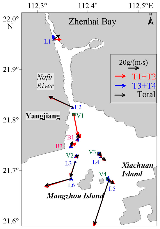
Figure 8.
Suspended sediment transport vector diagram at L1–L6, V1–V3, B1, and B3.
Table 5.
Suspended sediment transport rate and contribution of main transport terms. The ratio indicates the proportion of each flux to the sum of all flux magnitudes (Total) in the direction of Total, while the ‘−’ only represents the opposite direction of all sediment transport (Total). Unit of Flux, Direction (Dir), and ratio are g/(m.s), (°), and (%).
In spatial terms, stations L1 and L2, located in the river channel and near the outlet, experience landward transport sediment, whereas stations L3–L6 exhibit seaward transport sediment. Sediments are transported seaward at stations V1, V3, and V4, while sediment is transported landward at station V2. Sediment transports at stations B1 and B3, situated on the western shoal, are directed landward.
The magnitudes of single-width sediment transport are similar at stations L1–L6. Station L5, which is located near the open sea, exhibits the largest sediment transport value of 93.30 g/(m·s). The station with the smallest sediment transport value is station L4, situated to the northeast of Mangzhou Island, with a value of 11.85 g/(m·s). The advection term (T1 + T2) accounts for the largest proportion of the net suspended sediment transport at stations L1–L6. The tidal pumping effect term (T3 + T4) and vertical circulation term (T5) also influence suspended sediment transport, whereas the contribution of the shear diffusion term is minimal, with negligible impact on total suspended sediment transport within the study area. The direction of T1 + T2 is more consistent with the direction of total sediment transport. Except for station L1, the contributions of T1 + T2 to total sediment transport are greater than 99% for all stations. The proportion of T3 + T4 at station L1 is relatively large, indicating that the tidal cycle of tidal currents and suspended sediment varies greatly, and the asymmetry of tidal currents and suspended sediment is strong.
The magnitudes of the advection term (T1 + T2) are similar at all stations during 12–13 March 2013, and sediment transports are seaward at all stations except L2. Among sediment transport factors, T1 accounts for the largest proportion of the T1 + T2 term and is also the dominant factor driving the sediment-transport process. The direction of T1 is in accordance with Eulerian residual flow and is influenced by tidal deformation, runoff, and wind. Due to relatively low upstream runoff discharge and wind speed, the value of the T1 term primarily results from tidal asymmetry in the study area. Except at station L2, all stations are ebb-dominant, with T1 indicating sediment transport in the ebb direction toward the sea. The sediment transport direction indicated by T1 + T2 is seaward. Station L2, located near the outlet, experiences flood-dominant flow, resulting in T1 and T1 + T2 both indicating landward sediment transport. Spatially, sediment transport associated with Eulerian residual flow gradually weakens from the outlet toward the central estuarine bay. The magnitude of T2 reflects the correlation between tides and tidal currents. With the exception of station L5, proportions of total sediment transport in T2 term exceed 20% at all stations, signifying a notable correlation between flow velocity changes and water level variations. Except at station L3, the T3 + T4 term at each station is directed landward. Station L1, situated in the river channel, exhibits the highest T3 + T4 value of 8.31 g/(m·s). The next highest values are observed at stations L5 and L6, which are closer to the open sea, while the smallest values are observed at stations L2, L3, and L4. Except at station L5, the T4 term makes the greatest contribution to sediment transport in the T3 + T4 term, indicating that changes in SSC are primarily driven by variations in tidal current velocity. T5 term is directed landward at all stations and is closely linked to the mixing intensity. At station L1, located in the river channel with poor mixing, T5 accounts for the largest proportion of total sediment transport compared to other stations. The other stations exhibit strong vertical mixing, resulting in a diminished contribution of T5. The magnitudes of the T6 + T7 + T8 term are relatively small at all stations, representing the smallest proportion of total sediment transport.
In terms of spatial distribution, station V1, located near the outlet, exhibits the largest single-width sediment transport value of 41.73 g/(m·s) during 12–13 August 2022. The next largest value is observed at station V4, situated closer to the open sea, with a value of 15.47 g/(m·s). Stations V2 and V3 have the lowest single-width sediment transport values of 5.21 and 6.81 g/(m·s), respectively. Except at station V2, all stations are predominantly characterized by ebb-dominant flow. The factors driving sediment transport at stations at stations V1, V3, and V4 are in the order T1 + T2 > T3 + T4 > T5, while the order is T3 + T4 > T1 + T2 > T5 at station V2. T1 term is directed seaward at stations V1–V4; as it makes up the largest proportion of T1 + T2, T1 + T2 terms at these stations are all directed seaward. The direction of the T2 term is landward at stations V1, V2, and V4 and seaward at station V3. The T3 + T4 term is directed landward at stations V1, V2, and V3, while at station V4, it is directed seaward. The T3 + T4 term plays a smaller role than the T1 + T2 term. Except for station V2, the direction of T1 + T2 is consistent with the direction of the total sediment transport. Station V2 has a large proportion of T3 + T4 and a strong asymmetry between the tidal current and suspended sediment. Of the factors within T3 + T4, T4 makes the largest contribution, indicating that changes in SSC are primarily influenced by variations in the tidal current velocity. The values of T5 and T6 + T7 + T8 terms are relatively small at all stations, and these terms contribute little to sediment transport.
The factors driving sediment transport at stations B1 and B3 follow the following order: T1 + T2 > T3 + T4 > T5. The values of the advection term (T1 + T2) at stations B1 and B3 are similar, with station B1 having a slightly higher value than station B3. T1 accounts for the largest proportion of sediment transport impact factors, followed by T2. Both stations B1 and B3, located on the western shoal, experience flood-dominant flow, and the sediment transport direction of T1 is landward. The T5 term is directed landward at stations B1 and B3, and their contributions to sediment transport are similar, indicating comparable mixing conditions at these two stations. T3 + T4 transport sediment landward at station B1 and seaward at station B3. T4 accounts for the largest proportion of T3 + T4, indicating that changes in SSC are primarily influenced by variations in tidal current velocity. The T1 + T2 term is more important than the T3 + T4 term, and the transport direction is consistent with total sediment transport. The direction of T3 + T4 at station B1 is consistent with the total sediment transport direction, while opposite at station B3. Values of T6 + T7 + T8 are similar at stations B1 and B3 but are directed seaward at B1 and landward at B3. These terms make significant contributions to total sediment transport, both exceeding 16%. T8 makes the largest contribution to T6 + T7 + T8, indicating a significant effect of vertical tidal oscillation shear.
5. Discussion
5.1. Formation of Strong Mixing in Microtidal Estuaries
A microtide is typically defined by tidal amplitudes less than 2 m [30]. Based on the average amplitudes of stations Z1–Z4 for a month being 1.81 m, 1.56 m, 1.52 m, and 1.68 m, ZHE is a microtidal estuary. Mixing conditions of ZHE were assessed using the stratification coefficient N, tidal mean values of the potential energy anomaly (ϕ), and time derivative of ϕ. This study focused on the occurrence of strong mixing during spring tides in a microtidal estuary. When strong mixing does not occur during spring tides, it is highly unlikely to occur during other periods. Except at stations L1 and V1, all stations had negative mean values of (∂φ/∂t)total, indicating predominant mixing. However, stations L1 and V1, characterized by deeper water depths (with average values of 8.6 m and 8.6 m) and being located farther upstream, exhibited the largest vertical density gradient and significant estuarine circulation, resulting in positive mean values of (∂φ/∂t)total. Tidal average stratification coefficients N were < 0.15 at all stations, indicating that the mixing condition of each station is well mixed according to Prandle’s criteria [22], which is in agreement with tidal mean values of ϕ [26]. The mechanism of tidal stirring is revealed as a major reason for the occurrence of strong mixing in a microtidal estuary. Strong tidal stirring is attributed to low upstream runoff, a trumpet-shaped estuary, and a shallow water depth.
The influence of upstream runoff is relatively small, with annual mean discharge from Nafu River being < 100 m3/s. Therefore, the impact of runoff on the estuary is weak, and the tidal effect is strong. Tidal dynamics are the fundamental driver of mixing within the estuary, as supported by analysis of measured data, which indicated that tidal stirring dominates at all stations.
The convergence effect of the trumpet-shaped estuary has a significant influence on mixing conditions. Tidal energy gradually increases from the outer estuary to the inner estuary, leading to enhanced mixing. ZHE exhibited an exponentially narrowing boundary, characterized as , where y represents the width of the estuary, x represents distance along the estuary in the upstream direction, and the contraction index β is 0.1839. Based on the average tidal range calculated from the water level on 12–13 March 2013, the average tidal range is 1.9, 2.0, 2.4, and 3.4 m at stations L6, L3, L2, and L1 (from south to north), respectively, indicating that tidal energy increases upstream within the estuary. As tidal action intensifies, the interaction between water flow and the bed increases, resulting in strong stirring. The absolute value of the tidal stirring term at each station was generally consistent with the variation in the tidal range.
The shallow water depth within the estuary enhances vertical mixing. The impact of the water depth on various mixing factors can be analyzed through a comparison among stations. The stations selected for this analysis, located from the river channel through the outlet to the open sea, were stations L1, L2, L3, and L6. The order of average water depths is L1 (8.6 m) > L2 (6.2 m) > L6 (5.5 m) > L3 (4.4 m). The average values of (∂φ/∂t)cir are consistent with the ranking of water depth, at 1.92, 0.60, 0.29, and 0.15 × 10⁻⁴ W·m−3, respectively. Stations with deeper water depths exhibit larger (∂φ/∂t)cir values, which promote stratification. In contrast, shallower areas are more favorable to mixing. The tidal straining and tidal stirring terms are more closely related to tidal energy than to water depth.
Microtidal estuaries, such as the Lingdingyang Estuary, Huangmaohai Estuary, Passaic Estuary, York Estuary, and Sydney Harbour Estuary, are generally partially mixed or stratified [14,31,32,33]. For example, the Huangmaohai Estuary is a funnel-shaped microtidal estuary located along the southwestern side of the Pearl River Delta complex that is partially mixed to highly stratified during the wet season and well mixed to partially mixed during the dry season [14]. During the dry season in Huangmaohai Estuary, the mean sediment transport is landward in the channel and seaward on the shoals. Enhanced mixing can result in a predominantly seaward transport. Conversely, weak mixing can result in an emphatic landward transport. The York River is a partially mixed, microtidal estuary. Fluctuations in salinity stratification in the York River at tidal and seasonal timescales are associated with tidal straining and variations in freshwater discharge, respectively [31]. During spring tide, there was significant up-estuary sediment pumping in the channel with down-estuary pumping over the shoals [34]. Meanwhile, ZHE, another microtidal estuary, is well mixed during all three observation periods during both the wet and dry seasons. The key factor driving this difference is the moderating effect of geomorphology on hydrodynamics.
5.2. Effects of Mixing on Sediment Transport
Relatively high SSCs appear both in the surface and bottom layers of the water column during most periods of the three observations, which is attributed to the direct effect of strong mixing. Suspended sediment concentrations between the surface and bottom layers of the water column show minimal differences, which can be attributed to strong vertical mixing, facilitating frequent sediment exchange between the layers. The shallow water of ZHE also contributes to the resuspension of bottom sediment, raising it to the surface layer of the water column. High SSCs occur around the periods of peak flows, corresponding with tidal stirring.
Strong mixing leads to the control of residual sediment mainly by advective transport (T1 + T2). The proportion of advective transport varies through differences in tidal energy and tidal disturbance intensity in different spatial locations. Vertical sediment transport shows a close relationship with mixing, which is induced by vertical density circulation. Enhanced vertical mixing diminishes the contribution of the vertical net circulation to the total sediment transport.
In three observations, the greater magnitudes of advective transport occur at stations L2 and V1, near the outlet, aligning with the conclusion that tidal energy reaches its peak at the outlet. Laterally, a higher proportion occurs on the western side of the estuary compared to the eastern side. Similarly, the values of stratification coefficients indicate stronger mixing on the western side than on the eastern side. In three observations, stations B1 and B3 exhibit the smaller magnitudes of the advective transport term and the higher proportions of the T5 term, which represents vertical sediment transport in the absolute value of suspended sediment transport. The ratios of bottom sediment concentration to surface sediment concentration are higher at stations B1 and B3 (1.73, 1.98), implying weaker vertical mixing of sediment. Stratification coefficients (N = 0.08, 0.15) and potential energy anomaly (ϕ = 7, 15) are the highest in the three observations, which indicates mixing at stations B1 and B3 are the poorest among the three observations.
The sediment transport direction at stations near the river channel area is landward, whereas stations on the western shoal transport sediment towards the land, and the remaining stations transport sediment seaward. The trumpet-shaped estuary facilitates sediment deposition toward the land in the river channel area. Sediment transport around the western shoal to the outlet area exhibits a counterclockwise rotation, resulting in the accumulation of sediment on the western shoal.
5.3. Implication for the Estuarine Management
The strong mixing favors sediment resuspension in ZHE, leading to the fast back-siltation of the sediment, so the excavation of the navigation channel in ZHE may cause serious sediment siltation, and the maintenance of the navigation channel may have a high cost. Thus, it is not suggested that the deep navigation channel passes the ZHE if the economic return from the navigation can not support the maintenance of the channel. Strong mixing favors the existence of the shoals and forms a large area of wetland in ZHE, which is important for ecological protection.
5.4. Limitations and Future Work
This study reports data for flow velocity, flow direction, salinity, and SSC during three spring tides, while data from neap and moderate tides were not collected. Thus, the investigation of mixing and sediment transport in ZHE during neap and moderate tides is worthy of further study. Research into neap–spring shifts using models is another promising future direction. In addition, the effect of waves on mixing was not considered in this study and should be studied in future work.
6. Conclusions
Longitudinally, the average ebb flow velocity gradually decreases in the down-estuary direction, while the average flood flow velocity gradually increases up-estuary, reaching its maximum at the outlet. The vertical average of SSC gradually decreases up-estuary, reaching its minimum at the outlet, and increases slightly in the upstream direction. The vertical mixing of salinity is relatively strong at all observation stations.
Laterally, with Mangzhou Island as the boundary, velocities are higher on the west side than on the east side. The vertical average SSC values are similar between eastern and western stations at similar latitudes. Salinity values are higher on the west side than on the east side. On the western side of the shallow shoal, the flood tide velocity is greater than the ebb tide velocity, and the average SSC is therefore higher during flood tide than during the ebb tide. High SSC occurs around the periods of peak flood and ebb flows, indicating a correlation between SSC and tidal variations.
ZHE is a funnel-shaped estuary influenced by a convergence effect driven by topography. Tidal energy gradually increases as the tide propagates into the estuary, leading to an increase in the tidal-stirring effect. According to stratification coefficient N and tidal mean values of ϕ, ZHE was well mixed during three observation periods. Tidal stirring plays an important role in mixing as the most significant factor and is primarily driven by tidal dynamics. Estuarine circulation is closely related to the water depth and the horizontal density gradient, serving as the primary dynamic mechanism promoting stratification. Tidal straining significantly alters the water column’s stratification or mixing state within a single tidal cycle, while its influence on the tidal mean is comparatively minimal. The range of tidal straining and tidal stirring is larger on the western side than the eastern side, while the range of tidal straining is larger in areas closer to the open sea.
Sediment transport is landward at stations located in the river channel, near the outlet, and the western shoal, while it is seaward at stations within the estuarine bay. Driven by mixing, the advective transport term (T1 + T2) is the primary factor influencing sediment transport in ZHE, except station V2. The directions of the T1 + T2 term are more consistent with the main directions of total sediment transport for all stations. And the tidal pumping term (T3 + T4) is the secondary factor, except for station L3.
Author Contributions
Conceptualization, Y.L. and L.J.; methodology, Y.L.; software, Y.L., D.L. and M.L.; validation, Y.L., D.L., M.L. and L.J.; formal analysis, Y.L.; investigation, Y.L., D.L., M.L., T.Z., E.H. and Z.Z.; resources, Y.L. and L.J.; data curation, Y.L.; writing—original draft preparation, Y.L.; writing—review and editing, Y.L. and L.J.; visualization, Y.L.; supervision, L.J.; project administration, L.J.; funding acquisition, L.J. All authors have read and agreed to the published version of the manuscript.
Funding
This study is funded by Southern Marine Science and Engineering Guangdong Laboratory (Zhuhai) (SML2020SP006; SML2023SP220) and grants by Guangdong Provincial Special key project of six Marine Industries in 2022 ‘Research on Three-dimensional Efficient Utilization of Marine Spatial Resources in Guangdong-Hong Kong-Macao Greater Bay Area’ ([2022]49).
Institutional Review Board Statement
Not applicable.
Informed Consent Statement
Not applicable.
Data Availability Statement
The data that support the findings of this study are available from the corresponding author upon reasonable request.
Acknowledgments
The authors are very grateful to providers of the datasets used. The authors express gratitude to the Editor and anonymous reviewers for their constructive comments and suggestions, which undoubtedly contributed to the improvement of the manuscript.
Conflicts of Interest
The authors declare no conflicts of interest.
References
- Kennish, M. Environmental threats and environmental future of estuaries. Environ. Conserv. 2002, 29, 78–107. [Google Scholar] [CrossRef]
- Wetz, M.S.; Yoskowitz, D.W. An ‘extreme’ future for estuaries? Effects of extreme climatic events on estuarine water quality and ecology. Mar. Pollut. Bull. 2013, 69, 7–18. [Google Scholar] [CrossRef] [PubMed]
- Dyer, K.R. Estuaries: A Physical Introduction; John Wiley & Sons: Chichester, UK, 1997; Volume 78, pp. 693–695. [Google Scholar]
- Defontaine, S.; Sous, D.; Morichon, D.; Verney, R.; Monperrus, M. Hydrodynamics and SPM transport in an engineered tidal estuary: The Adour river (France). Estuar. Coast. Shelf Sci. 2019, 231, 106445. [Google Scholar] [CrossRef]
- Gong, W.; Shen, J. The response of salt intrusion to changes in river discharge and tidal mixing during the dry season in the Modaomen Estuary, China. Cont. Shelf Res. 2011, 31, 769–788. [Google Scholar] [CrossRef]
- Perales-Valdivia, H.; Sanay-González, R.; Valle-Levinson, A. Effects of tides, wind and river discharge on the salt intrusion in a microtidal tropical estuary. Reg. Stud. Mar. Sci. 2018, 24, 400–410. [Google Scholar] [CrossRef]
- Prandle, D. Saline intrusion in partially mixed estuaries. Estuar. Coast. Shelf Sci. 2004, 59, 385–397. [Google Scholar] [CrossRef]
- Valle-Levinson, A.; Schettini, C.A.F. Fortnightly switching of residual flow drivers in a tropical semiarid estuary. Estuar. Coast. Shelf Sci. 2016, 169, 46–55. [Google Scholar] [CrossRef]
- Veerapaga, N.; Azhikodan, G.; Shintani, T.; Iwamoto, N.; Yokoyama, K. A three-dimensional environmental hydrodynamic model, Fantom-Refined: Validation and application for saltwater intrusion in a meso-macrotidal estuary. Ocean Model. 2019, 141, 101425. [Google Scholar] [CrossRef]
- Lupiola, J.; Bárcena, J.F.; García-Alba, J.; García, A. A numerical study of the mixing and stratification alterations in estuaries due to climate change using the potential energy anomaly. Front. Mar. Sci. 2023, 10, 1206006. [Google Scholar] [CrossRef]
- Otero, L.J.; Hernandez, H.I.; Higgins, A.E.; Restrepo, J.C.; Álvarez, O.A. Interannual and seasonal variability of stratification and mixing in a high discharge micro-tidal delta: Magdalena River. J. Mar. Syst. 2021, 224, 103621. [Google Scholar] [CrossRef]
- Shen, X.; Detenbeck, N.; You, M. Spatial and temporal variations of estuarine stratification and flushing time across the continental US. Estuar. Coast. Shelf Sci. 2022, 279, 108147. [Google Scholar] [CrossRef]
- Azhikodan, G.; Hlaing, N.O.; Yokoyama, K.; Kodama, M. Spatio-temporal variability of the salinity intrusion, mixing, and estuarine turbidity maximum in a tide-dominated tropical monsoon estuary. Cont. Shelf Res. 2021, 225, 104477. [Google Scholar] [CrossRef]
- Gong, W.; Jia, L.; Shen, J.; Liu, J.T. Sediment transport in response to changes in river discharge and tidal mixing in a funnel-shaped micro-tidal estuary. Cont. Shelf Res. 2014, 76, 89–107. [Google Scholar] [CrossRef]
- Allen, G.P.; Salomon, J.C.; Bassoullet, P.; Du Penhoat, Y.; de Grandpré, C. Effects of tides on mixing and suspended sediment transport in macrotidal estuaries. Sediment. Geol. 1980, 26, 69–90. [Google Scholar] [CrossRef]
- Azhikodan, G.; Yokoyama, K. Temporal and Spatial Variation of Mixing and Movement of Suspended Sediment in the Macrotidal Chikugo River Estuary. J. Coast. Res. 2015, 313, 680–689. [Google Scholar] [CrossRef]
- Mitchell, S.B. Turbidity maxima in four macrotidal estuaries. Ocean Coast. Manag. 2013, 79, 62–69. [Google Scholar] [CrossRef]
- Uncles, R.J. Estuarine Physical Processes Research: Some Recent Studies and Progress. Estuar. Coast. Shelf Sci. 2002, 55, 829–856. [Google Scholar] [CrossRef]
- Geyer, W.R. The importance of suppression of turbulence by stratification on the estuarine turbidity maximum. Estuaries 1993, 16, 113–125. [Google Scholar] [CrossRef]
- Jay, D.A.; Musiak, J.D. Particle Trapping in Estuarine Tidal Flows. J. Geophys. Res. 1994, 99, 20445–20461. [Google Scholar] [CrossRef]
- Scully, M.E.; Friedrichs, C.T. The influence of asymmetries in overlying stratification on near-bed turbulence and sediment suspension in a partially mixed estuary. Ocean Dyn. 2003, 53, 208–219. [Google Scholar] [CrossRef]
- Prandle, D.; Ryder, D.K. Comparison of observed (HF radar) and modelled nearshore velocities. Cont. Shelf Res. 1989, 9, 941–963. [Google Scholar] [CrossRef]
- Pu, X.; Shi, J.Z.; Hu, G.D.; Xiong, L.B. Circulation and mixing along the North Passage in the Changjiang River estuary, China. J. Mar. Syst. 2015, 148, 213–235. [Google Scholar] [CrossRef]
- Simpson, J.H.; Brown, J.; Matthews, J.; Allen, G. Tidal strain, density currents, and stirring in the control of estuarine stratification. Estuaries 1990, 13, 125–132. [Google Scholar] [CrossRef]
- Simpson, J.H.; Williams, E.; Brasseur, L.H.; Brubaker, J.M. The impact of tidal strain on the cycle of turbulence in a partially stratified estuary. Cont. Shelf Res. 2005, 25, 51–64. [Google Scholar] [CrossRef]
- Scottish Marine Assessment 2020. Available online: https://marine.gov.scot/sma/assessment/stratification-potential-energy-anomaly (accessed on 22 May 2024).
- Ingram, R.G. Characteristics of the Great Whale River plume. J. Geophys. Res. Ocean. 1981, 86, 2017–2023. [Google Scholar] [CrossRef]
- Uncles, R.J.; Elliott, R.C.A.; Weston, S.A. Observed fluxes of water, salt and suspended sediment in a partly mixed estuary. Estuar. Coast. Shelf Sci. 1985, 20, 147–167. [Google Scholar] [CrossRef]
- Moskalski, S.; Floc’h, F.; Verney, R. Suspended sediment fluxes in a shallow macrotidal estuary. Mar. Geol. 2020, 419, 106050. [Google Scholar] [CrossRef]
- Whitfield, A.; Elliott, M. Ecosystem and biotic classifications of estuaries and coasts. Treatise Estuar. Coast. Sci. 2011, 99–124. [Google Scholar] [CrossRef]
- Friedrichs, C. York River Physical Oceanography and Sediment Transport. J. Coast. Res. 2009, 57, 17–22. [Google Scholar] [CrossRef]
- Mathew, R.; Winterwerp, J.C. Sediment dynamics and transport regimes in a narrow microtidal estuary. Ocean Dyn. 2020, 70, 435–462. [Google Scholar] [CrossRef]
- Xiao, Z.Y.; Wang, X.H.; Song, D.; Jalón-Rojas, I.; Harrison, D. Numerical modelling of suspended-sediment transport in a geographically complex microtidal estuary: Sydney Harbour Estuary, NSW. Estuar. Coast. Shelf Sci. 2020, 236, 106605. [Google Scholar] [CrossRef]
- Scully, M.E.; Friedrichs, C.T. Sediment pumping by tidal asymmetry in a partially mixed estuary. J. Geophys. Res. 2007, 112, C07028. [Google Scholar] [CrossRef]


Disclaimer/Publisher’s Note: The statements, opinions and data contained in all publications are solely those of the individual author(s) and contributor(s) and not of MDPI and/or the editor(s). MDPI and/or the editor(s) disclaim responsibility for any injury to people or property resulting from any ideas, methods, instructions or products referred to in the content. |
© 2024 by the authors. Licensee MDPI, Basel, Switzerland. This article is an open access article distributed under the terms and conditions of the Creative Commons Attribution (CC BY) license (https://creativecommons.org/licenses/by/4.0/).