Abstract
Fast and accurate detection of ship objects in remote sensing images must overcome two critical problems: the complex content of remote sensing images and the large number of small objects reduce ship detection efficiency. In addition, most existing deep learning-based object detection models require vast amounts of computation for training and prediction, making them difficult to deploy on mobile devices. This paper focuses on an efficient and lightweight ship detection model. A new efficient ship detection model based on device–cloud collaboration is proposed, which achieves joint optimization by fusing the semantic segmentation module and the object detection module. We migrate model training, image storage, and semantic segmentation, which require a lot of computational power, to the cloud. For the front end, we design a mask-based detection module that ignores the computation of nonwater regions and reduces the generation and postprocessing time of candidate bounding boxes. In addition, the coordinate attention module and confluence algorithm are introduced to better adapt to the environment with dense small objects and substantial occlusion. Experimental results show that our device–cloud collaborative approach reduces the computational effort while improving the detection speed by 42.6% and also outperforms other methods in terms of detection accuracy and number of parameters.
1. Introduction
Ship detection plays a key role in maritime surveillance and protection of offshore installations [1,2,3,4]. The main purpose of ship detection is to identify the ship object, ship location, and ship type. Ship detection not only plays an important role in the automatic navigation, collision avoidance, and efficient communication of intelligent ships but also plays a key role in traffic management, safety supervision, environment protection, and emergency response in traffic supervision. The application of intelligent ship detection has greatly improved the efficiency and safety of maritime management and promoted the development of smart ships. With the development of deep learning methods and aerospace measurements, deep learning-based object detection models can quickly and accurately detect targets in remote sensing images and have been widely used in the military, navigation, rescue, and other fields [5,6]. Despite significant progress in deep learning-based object detection algorithms, they still face the challenge of high computation and memory resource consumption. First, we analyze the classification of existing deep learning-based object detection algorithms and their limitations. Existing deep learning-based object detection algorithms can be categorized into anchor-free, anchor-based, and Transformer-based methods [7,8,9]. The anchor-based method can directly classify the target and regress the bounding box, improving small object detection ability. However, it generates many redundant anchor boxes, increasing the computation and memory consumption. Although the anchor-free method predicts the target directly based on the feature map instead of a preset anchor box, it is more susceptible to noise interference, especially for remote sensing images. Remote sensing images have a complex structure and contain a large number of small objects. Fast and accurate ship detection in remote sensing images must overcome these factors’ interference. The detection model based on the Transformer architecture relies on the global attention mechanism, which needs to compute the relationship between all the positions [10]. This computation becomes particularly complex and time-consuming with large-size inputs (e.g., remote sensing images). The model contains a large number of parameters, so it suffers from the problems of slow convergence speed and insufficient detection performance of small targets. Therefore, designing an efficient and accurate remote sensing image ship detection model is an important research direction [11].
In addition, semantic segmentation of remote sensing images is an important research area closely related to object detection. Semantic segmentation aims to extract regions of interest in an image and determine the class attribution of each image pixel. Deep learning-based semantic segmentation algorithms are widely used for land classification of remote sensing images. Since ships involved in maritime safety do not appear in areas outside the water, ship detection calculations in remote sensing images do not need to consider areas outside the water. This provides a vital idea for improving the efficiency of ship detection computation in remote sensing images. The semantic segmentation and object detection models based on deep learning have a large number of parameters and require significant computing power support for the model training. This puts high requirements on ordinary mobile devices.
In this paper, we propose a novel and efficient ship detection framework based on device–cloud collaboration, which integrates joint optimization of semantic segmentation and object detection and migrates some tasks that consume a lot of computing and memory resources to the cloud. This distributed device–cloud collaborative computing approach enables our system to efficiently manage computing resources and computational loads while maintaining high-precision detection. By excluding the nonwater regions, the computation and postprocessing time for these areas can be saved, thereby improving detection accuracy and efficiency. The main contributions of this paper are as follows:
- A novel ship detection framework based on device–cloud collaboration is proposed, which integrates semantic segmentation and object detection functions. By migrating the segmentation module to the cloud, the semantic segmentation results are stored in the cloud for the device-end object detection exploitation to optimize the allocation and utilization of computational resources.
- A Mask module and Anchor Head module are designed to reduce the computation and postprocessing time of the network.
- The performance of semantic segmentation and ship detection is improved by joint training of semantic segmentation and object detection.
- The postprocessing step and loss function of the original YOLO model are improved. Additionally, a Coordinate Attention module is introduced to better adapt to environments with dense small objects and heavy occlusion.
- In order to verify the effectiveness of the proposed method, we have conducted extensive ablation and comparison experiments. The experimental results show that our device–cloud collaborative method significantly improves detection efficiency while ensuring detection accuracy.
The following sections are divided as follows: Section 2 describes previous work closely related to this research, including semantic segmentation, detection method, and device–cloud collaboration architecture. Section 3 describes our definition of ship detection for remote sensing images. Section 4 describes the method proposed in this paper, including the device–cloud collaboration framework, the Backbone structure of SD-Net, the Neck and Head structure, and some computation details. Section 5 introduces the experiments and analysis. Finally, Section 6 is the conclusion of this paper.
2. Related Work
In our framework, we use the semantic segmentation model to find the attention area and then the object detection model to obtain the final results. We also propose a new efficient computation framework based on device–cloud collaboration to integrate semantic segmentation and object detection. Therefore, this section mainly reviews the work on semantic segmentation, object detection, and device–cloud collaboration.
2.1. Semantic Segmentation in Remote Sensing Images
Currently, semantic segmentation methods based on deep learning can be divided into two main categories: one is based on the convolutional neural network, and the other is based on the Transformer network structure. Among these methods, convolutional neural networks are widely used to analyze land classification and land cover information in remote sensing images. FCN [12] is the first effective knot method to solve the semantic segmentation problem in an end-to-end way. However, it suffers from issues such as the loss of semantic information and the lack of correlation between pixels. To address these problems, researchers mainly explore three strategies: combination with traditional algorithms, multiscale methods, and data fusion. For the method combination, Shen and Gao [13] designed a semantic segmentation network based on DeeplabV3+ to enhance the accuracy of pixel classification of natural landform edges in remote sensing images by fusing the edge detection module. For the multiscale strategy, Li et al. [14] proposed a multi-field-of-view deep adaptive fusion network (MFVNet) to obtain different scales of views from multiple FOVs by pyramid sampling and select a scale-specific model to make the best prediction. Cai et al. [15] found that different classes of objects at different scales have their preferred resizing scales for more accurate semantic segmentation, leading to the proposal of a stack-based semantic segmentation (SBSS) framework that improves segmentation results. For the data fusion, Saralioglu and Gungor [16] used a 3D-2D convolutional neural network model that combines spectral and spatial information to improve the classification accuracy of high-resolution satellite images.
Recently, many works have applied the Transformer network architecture to semantic segmentation tasks, originally used to process and analyze sequence data. Wu et al. [17] proposed a semantic segmentation network fusing the convolutional neural network with a multiscale Transformer and constructed a Transformer decoder to perform semantic segmentation by processing the output features of the CNN encoder. Xiao et al. [18] proposed a novel hybrid architecture for HRRS image segmentation, combining the advantages of convolutional network and Transformer to enhance multiscale representation learning. He et al. [19] proposed a novel framework for semantic segmentation of remote sensing images by embedding Swin Transformer into the classical CNN-based UNet.
2.2. Ship Detection in Remote Sensing Images
Detecting ships in remote sensing images is a challenging task. Deep learning-based methods have made significant progress. We only list the work that is more relevant to our research. For the simplification of detection, researchers have proposed ideas similar to our method. They use different strategies to reduce the computational effort of detection, including step-by-step filtering and information fusion. Li et al. [20] first distinguished suspicious regions from images based on the Hue, Saturation, and Value (HSV) differences between the ship and the background and extracted regions of interest from the input image. Then, they designed an improved YOLO algorithm based on a high-resolution image network algorithm to match candidate ships more efficiently. To expel false candidate targets in nontarget regions, You et al. [21] improved the detection accuracy and reduced false alarms by combining a near-shore scene mask with the detection framework. In addition, Tian et al. [22] proposed a small two-stage detection method. Candidate region extraction is first performed to localize potential ship locations, and then detection calculation is conducted. Liu et al. [23] proposed an unsupervised deep learning ship depth estimation method for sensing images. Thus, ship detection can fuse the depth information. However, these methods lack careful consideration for the deployment of lightweight front ends.
For lightweight ship detection models, researchers have also conducted extensive work based on the YOLO model for lightweight ship detection. The authors in Xu et al. [24] proposed a lightweight shipboard SAR ship detector based on the YOLOv5 algorithm, reducing the computation and improving detection performance through network pruning and multimodule integration. The WGC-PANet proposed in [25] reduces the model parameter and computational complexity to ensure the light weight of the network. Peng et al. [26] offered a lightweight YOLO (AMFLW-YOLO), which reduces the model parameter by employing depth-separable convolution and introducing Coordinate Attention (CA) modules and bidirectional feature pyramids to enhance feature extraction. Liu et al. [27] proposed a lightweight ship detection model based on joint optimization of defogging and detection, which has improved the YOLOv5s model.
2.3. Cloud Computing and Device–Cloud Collaboration
With the widespread application of deep learning models, the computational power of the front end makes it difficult to meet the growing computation demand of deep learning, leading to a decrease in model training accuracy and prediction efficiency. However, cloud computing technology has been widely used and has demonstrated flexible and powerful computing capabilities. To improve the front end’s computational efficiency and storage capacity, researchers have begun to utilize cloud computing to design device–cloud collaboration frameworks to solve problems with extensive computation and storage demands.
Regarding computing power optimization, current research focuses on computing power architecture design, computing offloading, and model decomposition. To alleviate the problem of limited computational capacity of edge servers, Liu et al. [28] constructed a hybrid computing task offloading architecture for cloud–edge–terminal collaboration and proposed a multiobjective offloading algorithm SPMOO based on the improved Strength Pareto Evolutionary Algorithm SPEA2, which aims to optimize the average latency and energy consumption of complex dependent tasks. Liu et al. [29] investigated joint task offloading and resource allocation for cloud–edge–terminal collaboration by formulating a new optimization problem to minimize the task processing delay. Zhuang et al. [30] proposed a novel module-level model decomposition design that decomposes the cloud model into multiple composable submodules, enabling it to generate compact, task-specific submodels for different edge devices. In terms of application, researchers have also conducted many valuable explorations. Based on the concept of cloud–edge–terminal collaboration, Wang et al. [31] proposed a four-layer networked architecture that breaks through traditional battery management systems’ computational power and storage space limitations. Zhang et al. [32] proposed a device–cloud collaboration-based fault detection model with a stacked auto-encoder deep neural network (SAES-DNN). The model is trained in the cloud and deployed on the front end through a transfer learning strategy. Tan et al. [33] designed user experience metrics to measure object detection and energy consumption comprehensively, then proposed an adaptive scheduling algorithm to schedule object detection and tracking tasks through network bandwidth and transmission delay prediction.
3. Definition of the Problem
In port and waterway areas where ship management is required, front-end equipment obtains real-time images to detect ships. However, ship targets only exist in water areas, so nonwater information in images is redundant. This redundant information increases the amount of calculation required for ship detection, which in turn increases the computing power consumption of front-end equipment. Therefore, this paper mainly focuses on the high complexity and high consumption of front-end detection calculations, especially for ship monitoring of UAV applications. Existing ship detection models are large, consume a lot of power, and run on high-performance computers. However, when front-end equipment such as UAV performs ship detection, it faces limitations in terms of chip computing efficiency, power consumption, storage capacity, and network capacity. Specifically, the limitations can be described as follows:
- Chip computing efficiency affects the speed of ship detection.
- Power consumption affects the working time of front-end equipment. For example, the maximum flight time of the DJI Mavic 3E is 45 min.
- Storage capacity affects the detection capacity and range of front-end equipment. For example, the storage capacity of DJI Mavic 3E is usually 512 GB.
- Network capacity affects the speed at which information can be transmitted.
To deal with these limitations, we redefine the remote sensing image detection problem under the device–cloud collaborative framework, refine the calculation process, improve the accuracy of each subprocess, reduce the front-end calculation amount, and achieve fast and accurate ship detection.
Definition 1.
Detection model .
Since ships involved in maritime safety do not appear in regions other than water, focusing our attention on the water region can effectively reduce unnecessary computations and thus improve the efficiency and accuracy of the overall detection process. Therefore, ship detection does not need to consider regions other than water, and ship detection can be categorized into semantic segmentation , object detection in water region , and object detection in the nonwater region .
Definition 2.
Semantic segmentation .
Semantic segmentation determines the category to which each pixel of the image belongs. We first categorize the pixels of remote sensing images by semantic segmentation to distinguish between water and nonwater areas.
Definition 3.
Object detection in water .
In the water region of the image, we perform ship detection.
Definition 4.
Object detection in nonwater .
In the nonwater region of the image, ship detection is not performed by utilizing semantic features and mask images, thus reducing the amount of computation.
4. Methodology
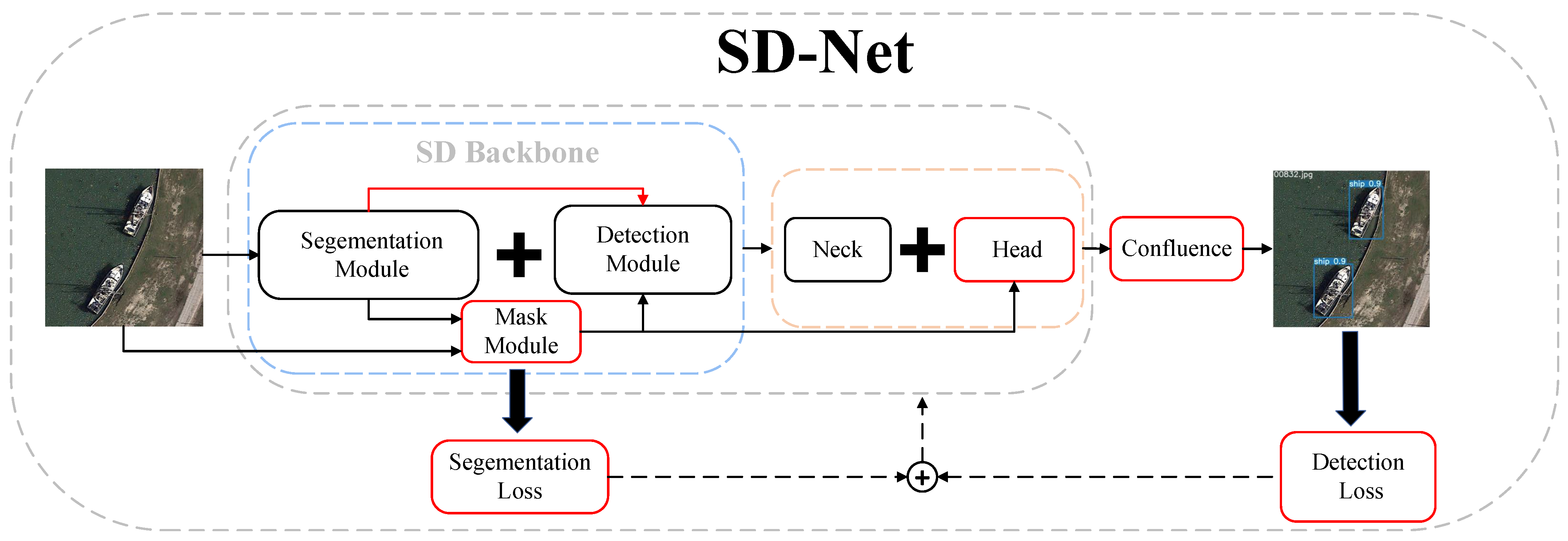
To efficiently process remote sensing images and improve the accuracy of ship detection, we design a novel joint optimization network for semantic segmentation and object detection (SD-Net, shown in Figure 1). The network is capable of joint training and can be deployed separately to achieve low coupling between modules. We introduce residual connectivity between the segmentation and detection modules and use the -IoU loss as the regression loss for the bounding box to ensure that the network converges stably. Considering the dense targets and severe occlusion in remote sensing images, we use the Confluence algorithm as a postprocessing step for ship detection. In the head layer of the detection network, we integrate the CA (Coordinate Attention) module to improve the model’s sensitivity to the target location and the detection accuracy. In addition, we design the Mask module and Anchor Head module to reduce the computation of network convolution operation and the number of candidate bounding boxes based on the mask feature, thus reducing the overall computation and postprocessing time.
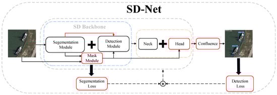
Figure 1.
Schematic diagram of SD-Net network structure. Solid arrows indicate forward processes and dashed arrows indicate backward processes. The red boxes are the main modules designed in this paper. The red arrow denotes the residual connection we designed.
In this paper, the device–cloud collaboration computation framework is used to place each subprocess of the detection model either in the cloud or in the front end, depending on its computation characteristics. We first describe the device–cloud collaboration framework and then explain the structure of our proposed SD-Net network and the improvements to the YOLO model.
4.1. Device–Cloud Collaboration Framework
With the rapid development of cloud computing, massive computing programs can be split into smaller subtasks. This advancement provides new opportunities for our ship detection research, which is very important for the front end in the 5G era. First, most front ends have relatively low computational power and small storage capacity. However, model training and model prediction of the deep learning-based semantic segmentation and object detection tasks require high computing power and large storage capacity. In order to reduce the computing consumption of the front end, some tasks that consume a lot of computing and memory resources should be migrated to the cloud. Second, the computing property of each task is different. Semantic segmentation can be defined as a “one-time calculation”. That is, after the input image has undergone a semantic segmentation operation, the optimized results can be retained for subsequent operations. The ship detection calculation can use the obtained results to identify ship objects in the water area. However, object detection in this paper is defined as “repetitive calculation” because this calculation will be repeated for each input image.
Based on the above analysis, we designed a device–cloud collaboration framework for ship detection, which migrates operations that require lots of computing and memory resources to the cloud. Specifically, we assign the “one-time calculation” and the corresponding output to the cloud side and assign the “repetitive calculation” that can be run directly on the front end and the corresponding output to the front end.
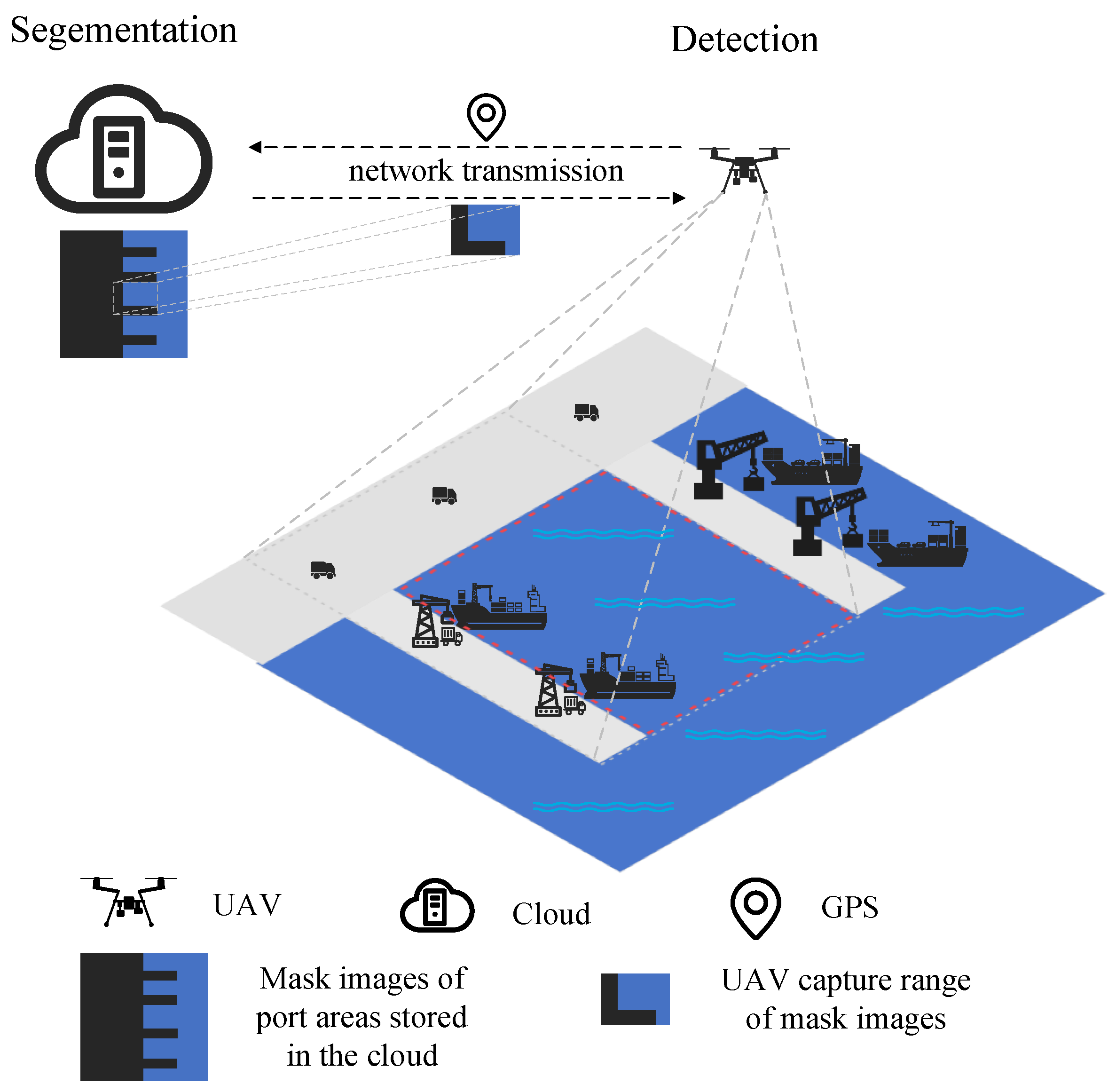
In the cloud, we train SD-Net by cloud computing, and then we divide SD-Net into two modules: one module is used for semantic segmentation, and the other is used for ship detection. Since the range of the detection area is usually administratively fixed, the cloud-first performs semantic segmentation on the remote sensing images of the detection area to distinguish between water parts and nonwater parts and stores the obtained mask images in the cloud. Figure 2 shows our device–cloud collaboration scenario. Under good weather conditions, normal 5G network, and normal operation of the device–cloud devices, when the front-end device (UAV) reaches a certain location in the surveillance area, it uploads the current location information to the cloud. After receiving the location information, the cloud sends mask images of the corresponding area to the front end. By applying these mask images to the real-time images, the front-end device is able to reduce the convolution operations in nonwater areas and reduce the number of candidate bounding boxes generated in the nonwater part of the network, thus reducing the overall computation and shortening the postprocessing time. Based on this distributed computing approach, our framework can effectively manage the computational load while maintaining high detection accuracy.

Figure 2.
Schematic diagram of the device–cloud collaboration scenario. The area surrounded by the gray dashed line is the detection area of the UAV, and the area surrounded by the red dashed line is the water area.
4.2. Backbone Structure
4.2.1. Basic Module
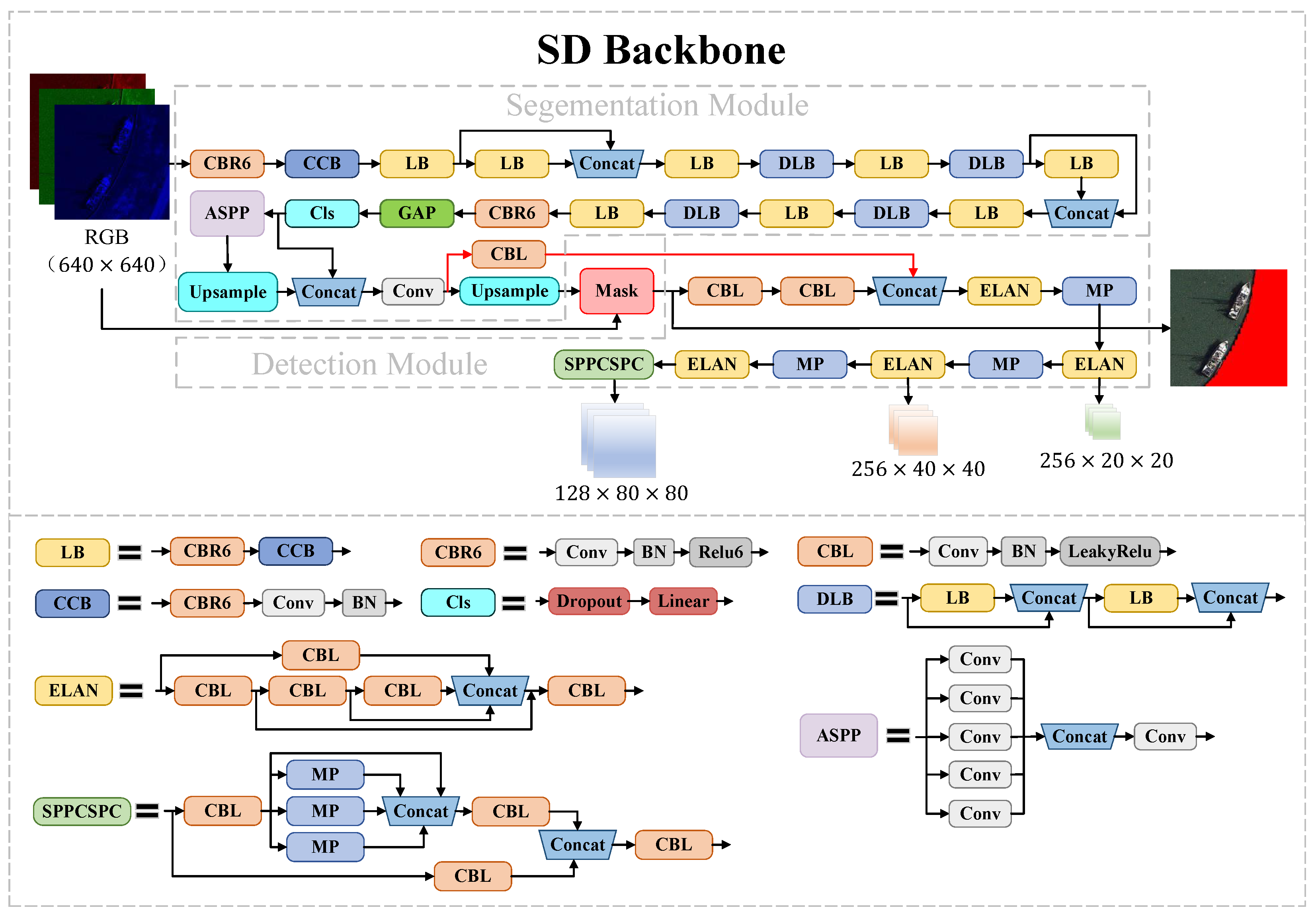
In this paper, we design our SD Backbone with reference to the ideas of DeepLab [34] and YOLO [35] models. As shown in Figure 3, the Backbone structure fuses multiscale information to improve the accuracy of segmentation based on an Atrous Spatial Pyramid Pooling Integrated (ASPP) module [36]. By applying multiple parallel null convolutions with different sampling rates, the ASPP module can increase the receptive field while maintaining information integrity, which is especially important for distinguishing targets of various sizes. The features extracted at each sampling rate are further processed in separate branches to obtain multiscale object information. The Efficient Layer Aggregation Networks (ELAN) module is a critical component of our network, which enhances the network’s learning capability and robustness by controlling the shortest and longest gradient paths. In addition, we also use the Spatial Pyramid Pooling and Fully Connected Spatial Pyramid Convolution (SPPCSPC) module, which reduces the computation and improves the processing speed and accuracy.

Figure 3.
Diagram of the SD Backbone Network. The land area where the mask is added in the remote sensing image is marked in red.
To avoid the vanishing and exploding gradient problem, we design residual connections between the segmentation module and the detection module (the red solid lines shown in Figure 3), which help to optimize the stability of the network training.
4.2.2. Mask Module
We design a Mask module to filter the input image based on the semantic segmentation results and fuse the semantic feature. By analyzing the elements on the feature map and their corresponding positions on the original map, we decide whether to perform subsequent convolution operations or not. For regions that are not within the watershed, we do not process the convolution operation, significantly reducing the computational effort of the network by this method. It can optimize not only the detection calculation but also the segmentation results. The Mask module can be represented by Equation (2).
where I denotes the input image, denotes the pixel value of the image at , M is the mask image, is the pixel value of the mask image at , is the output image after adding mask, and denotes the pixel value of the image at . The use of the Mask module is described in Section 4.3.2.
4.3. Neck and Head Structure
4.3.1. Basic Module
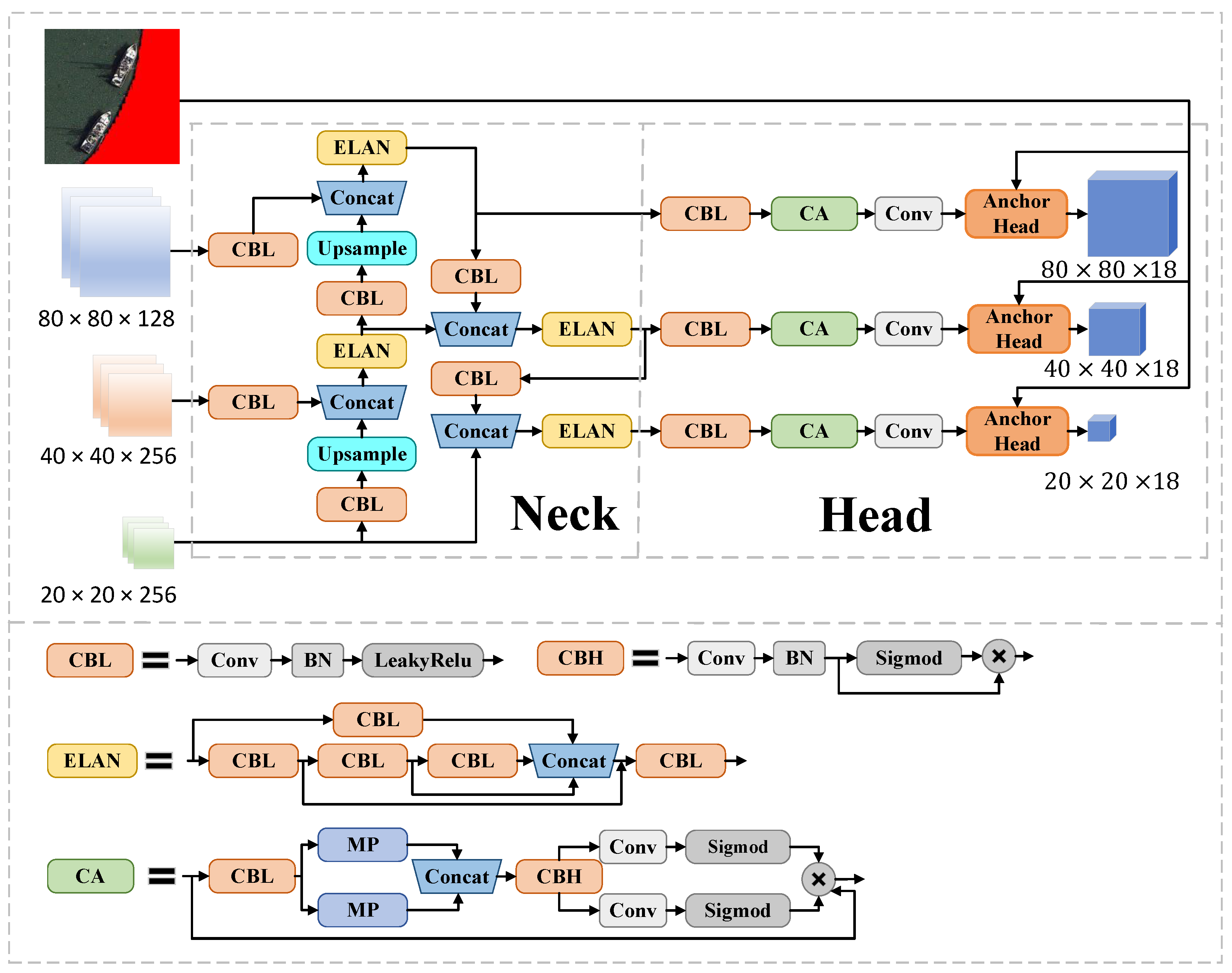
To fully utilize the feature information extracted from the SD Backbone and the masked images, we design a network structure to integrate the aspects of information, as shown in Figure 4. It can integrate three-scale feature information output from Backbone to achieve more effective object detection. Specifically, our strategy is to perform object detection on three different scale feature maps, feature map for small object detection, feature map for medium-sized object detection, and feature map for large object detection. This multiscale detection approach allows the model to recognize and distinguish between targets of different sizes more accurately. Last, we use feature fusion and multiscale processing methods to improve the detection efficiency for the complex content of remote sensing images.
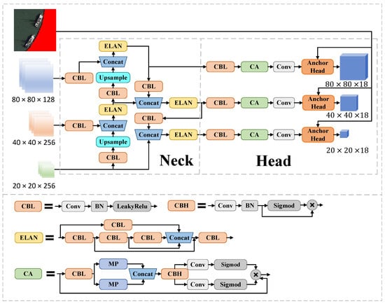
Figure 4.
Diagram of Neck and Head network structure. The land area where the mask is added in the remote sensing image is marked in red.
4.3.2. Anchor Head Module
The postprocessing step usually requires a lot of computing resources. Optimization of this step is crucial in the object detection process. To address this challenge, we design a novel Anchor Head module in the detection head section for fusing semantic features and generating candidate bounding boxes only in the water portion, thus reducing the computational effort. This process can be described by Equations (3) and (4).
where is the coordinate position of the centroid of the kth grid, L denotes the pixel of the water portion, is an indicator function of whether the centroid of the kth grid is in the water or not, and T is a threshold for determining whether or not to generate a candidate bounding box, we set in this paper. We not only consider whether or not the current grid’s centroid is in the water but also consider the states of the neighboring locations. This provides a more nuanced and dynamic way of determining whether to generate a candidate bounding box in the current region. The Anchor Head module determines whether to generate a candidate bounding box and thus decides whether to conduct a prediction.
4.4. Coordinate Attention Module
The attention mechanism focuses on localization information, which can suppress useless information and amplify useful information. Therefore, incorporating the attention mechanism can effectively enhance the extraction of localization features from the region of interest. Because the ship targets in remote sensing images are often small and dense, we add an efficient CA module [37] in the Head layer, which embeds the position information into the channel attention so that the model can more accurately locate and recognize the ship in the water area with little computation load. The processing of the CA module is as follows:
The input x is first subjected to a global pooling operation in the horizontal and vertical directions to produce the outputs and , respectively. These two features are subsequently spliced along the spatial dimension and fed into a convolution layer. The output of the convolution layer is processed through a sigmoid activation function, and the generated features are then divided into two parts along the spatial dimension: and .
By feeding and into a convolution layer, the attention weights and will be obtained followed by a sigmoid function. Each element in the attentional feature maps and reflects whether the ship object of interest is present in the corresponding row and column. This encoding process allows our coordinate attention to more accurately localize the exact location of the ship, which in turn helps the overall model to identify the ship better. and will be multiplied with the original input x to generate coordination features.
The CA module decomposes channel attention into two 1D feature encoding processes that aggregate features along different directions. Long-range dependencies are captured along one direction, and precise location information is retained along the other spatial direction. The output feature maps are then encoded separately to form a pair of direction-aware and location-sensitive feature maps, which can be applied complementarily to the input feature map to enhance the representation of the interest target.
4.5. Postprocessing Design
The YOLO model uses the NMS algorithm to retain the bounding box. However, NMS [38] relies heavily on the classification confidence score to determine the optimal box, which is not always an effective description of localization accuracy. Ship targets in remote sensing images are usually small, densely distributed, and often occluded. The NMS algorithm leads to significant problems of missed and false detections. In order to deal with these small and dense targets more effectively, we adopt the Confluence algorithm [39] as the postprocessing step of the network.
The Confluence algorithm reduces unnecessary bounding boxes while preserving key detection results. The confidence-weighted Manhattan distance is first used to assess the similarity between different candidate bounding boxes. Then, dense clusters are obtained based on normalized proximity metrics. An optimal box is selected where the gradient converges to zero, and other bounding boxes fused with the optimal box are removed. Rather than simply suppressing a large number of detection results, the Confluence algorithm determines the optimal box by identifying the box that intersects the most with other bounding boxes. As a result, this algorithm reduces the likelihood of false detections and thus improves the overall accuracy. It is more robust when dealing with densely distributed and small targets.
The Manhattan distance is the sum of the vertical and horizontal distances between two points, and the Manhattan distance between point and point is calculated according to Equation (9).
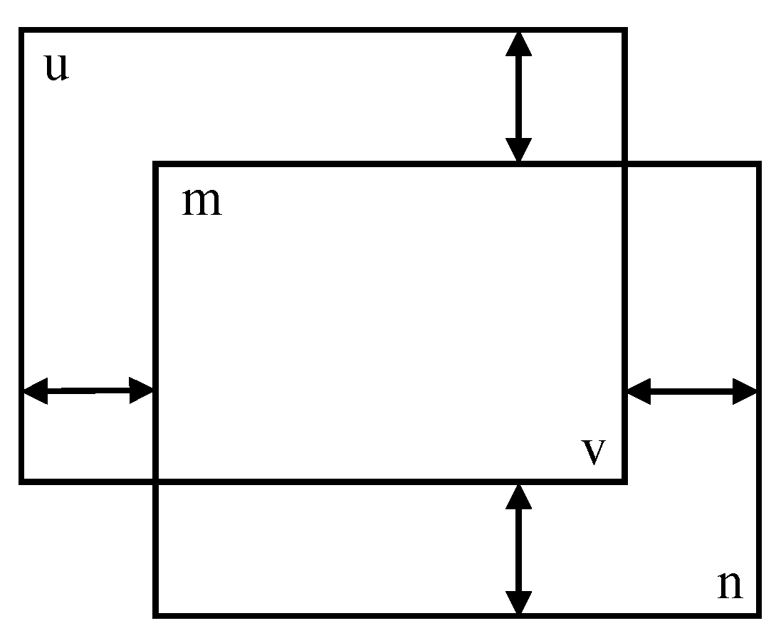
The proximity measure between two candidate bounding boxes can be expressed as the sum of the Manhattan distances of the upper-left and lower-right points (as shown in Figure 5). It is calculated according to Equation (10).
where is the proximity measure between the two candidate bounding boxes, is the Manhattan distance between the upper left corner points of the two boxes, and is the Manhattan distance between the lower right corner points of the two boxes. P denotes the degree of intersection of two frames. A larger P indicates that two frames are less likely to represent the same object. For frames within a cluster, we take the frame with the smallest intra-cluster P-value as the best frame. Considering that different frame sizes may result in particular sensitivity to the threshold parameter, the P-value between any two intersection frames will be less than two by normalizing all coordinates to a range from 0 to 1. Thus, if the P-value between two frames is less than 2, they can be considered to belong to the same cluster. Once the clusters are identified, the optimal intracluster boxes can be determined. Next, a threshold is set to eliminate false detections by removing all boxes that have a P-value less than this threshold with the optimal box. This process is repeated for all candidate boxes to optimize the overall detection.

Figure 5.
Schematic diagram of the Manhattan distance between two bounding boxes.
4.6. IoU Loss Design
Remote sensing images contain both small and large ship targets. In order to enable the model to adapt to different types of targets, we use -IoU loss [40] to enhance the sensitivity of the loss function to bounding boxes of different sizes and aspect ratios. This does not add additional training parameters and does not increase the computation burden. The Loss is defined according to Equation (11).
where is a positive parameter. Most of the existing loss functions can be derived by adjusting the value of . The -IoU loss in the two cases of and is calculated according to Equation (12).
For the case of , the -IoU loss under the condition of can be extended to a more general form by introducing a power regularization term (as shown in Equation (13)).
where , B and are the predicted box and the ground truth, respectively, and is a penalty term calculated according to B and .
When , the loss function will focus more on high IoU objects by increasing the weight of their relative loss. Thus, it helps the object detector to learn objects with a high degree of IoU faster. At the same time, the absolute amount of loss increased by is more conducive to optimizing objects at all levels.
4.7. Joint Optimization
Object detection and semantic segmentation are two separate remote sensing image processing tasks. However, these two tasks are closely related: accurate segmentation can help object detection to localize objects more accurately, while effective object detection can provide essential clues about object classes in the segmentation task. By integrating object detection and image segmentation in a unified framework, joint optimization of the two tasks can be achieved with the help of information flow between them.
We use a joint loss function to guide this joint optimization process. The joint loss function is shown in Equation (14).
where is the segmentation loss, is the detection loss, and is the weight parameter. At the beginning of training, we prioritize accurate segmentation since it is essential for subsequent ship detection. We set the initial value of to a high value of 0.9. As the training progresses, this weight is gradually reduced to 0.5. This strategy first ensures high-quality segmentation results and then gradually enhances ship detection, thereby achieving an effective balance between the two tasks.
The segmentation loss includes CE Loss and Dice Loss. The former calculates the loss of each pixel equally, and the latter can alleviate the negative impact of foreground and background imbalance in the dataset. The two losses are calculated according to Equation (15) and Equation (16), respectively.
where is the label, is the prediction result, and N is the number of pixels. The detection module uses the -IoU loss (as in Equation (11) to accurately assess the degree of overlap between the predicted bounding box and the ground truth and uses BCE Loss to assess the probability of the presence of the detected target. The BCE Loss is calculated according to Equation (17).
where is the label, is the prediction result, and M is the number of targets. Based on this joint optimization, the information flow between these two tasks forms a positive feedback loop, making the two tasks more accurate and effective.
5. Experiments and Analysis
5.1. Implementation Details
5.1.1. Dataset
The first challenge of this research is that few datasets are dedicated to both ship detection and semantic segmentation. To address this issue, we construct a new dataset based on publicly available datasets, including DIOR [41], DOTA [42], and LEVIR [43]. We select remote sensing images labeled with “ship” and exclude all nonship remote sensing images. Then, we label these remote sensing images with water and nonwater areas. The newly constructed dataset contains 2891 images. We divide these data into training and validation sets in the ratio of .
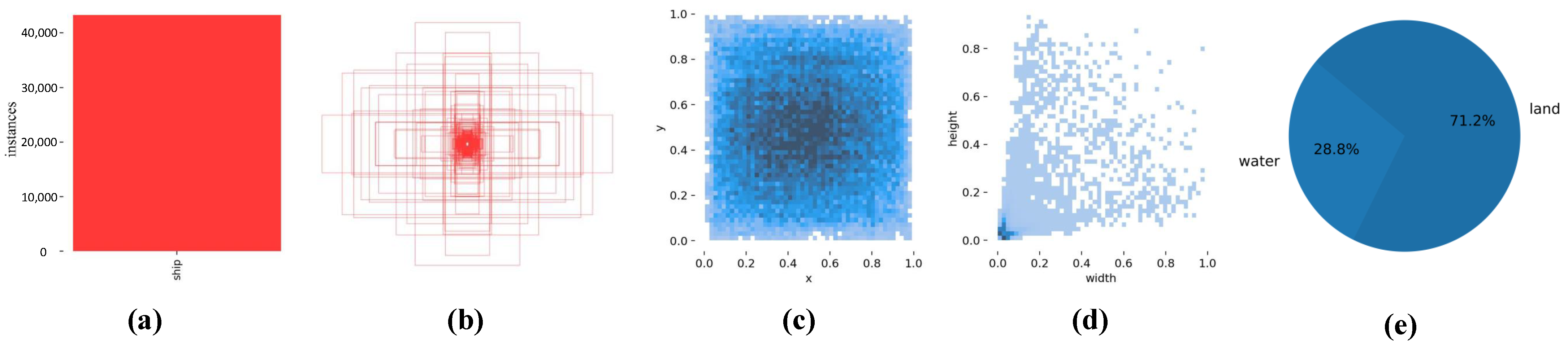
Figure 6 shows the visual analysis of our dataset. Figure 6a shows that there are more than 40,000 ship instances in our dataset. Figure 6b shows the sizes and numbers of all our ground truths. Figure 6c is the distribution of the centroids of ground truths with respect to the position of the whole image, and it can be seen that most of the instances are concentrated in the central region of the image. Figure 6d shows the distribution of the number of different instances, and it can be seen that the majority of instances of the dataset are small ships. Figure 6e shows the distribution of water and nonwater pixels in the dataset. The water portion can account for about one-third of the dataset.

Figure 6.
Dataset visualization: (a) Number of ship instances, (b) the distribution of ground truths, (c) the distribution of instance center points, (d) the distribution of instance sizes, and (e) the proportion of water and land areas. The darker the color of the point, the more the number of instances in (c,d).
5.1.2. Model Training
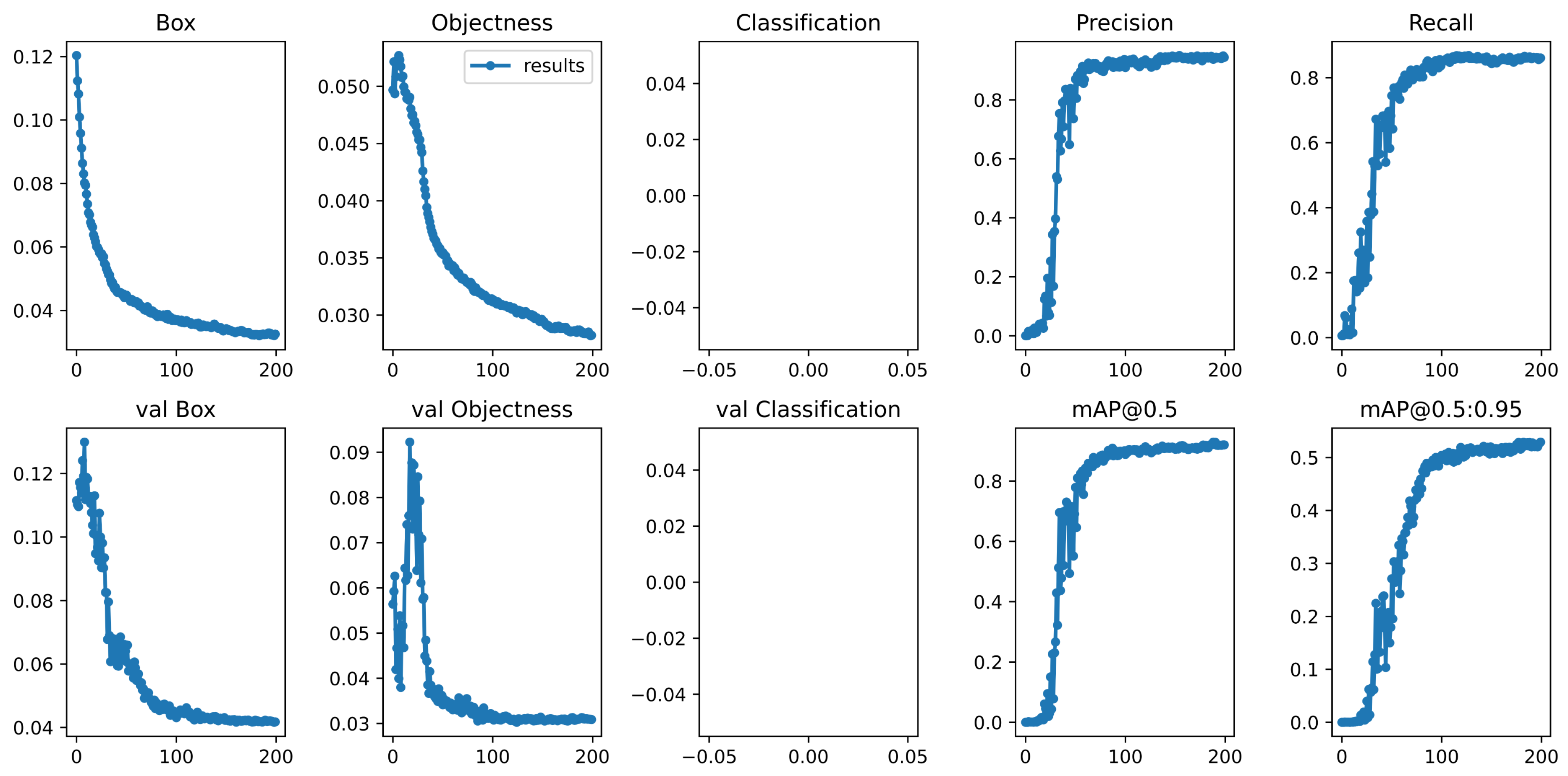
During the training process, we first resize the images to a uniform size of . We employ various data enhancement methods, including image flipping, affine transformation, and Gaussian blurring, to further enhance the model’s generalization ability and robustness. We use Stochastic Gradient Descent (SGD) as the optimizer and train the model for 200 epochs with a starting learning rate of 0.01, weight decay of 0.0005, batch size of 32, and cosine annealing used to adjust the learning rate dynamically. All experiments are conducted based on the Pytorch framework and run on NVIDIA 4090 GPU. We use the constructed dataset to train our model and the validation set to validate the results of each epoch during model training. Figure 7 shows the graphs of Box loss (Box), Objectness loss (Objectness), Classification loss (Classification), Precision, Recall, mAP@0.5, and mAP@0.5:0.95 during the training of our model. Since we are testing for only one category, ships, the category loss is not recorded. As shown in Figure 7, the val box loss and val Objectness loss drop rapidly in the first hundred epochs and then stabilize. From Figure 7, mAP@0.5 and mAP@0.5:0.95, we can see that our model can obtain good detection results, and there is no overfitting problem.
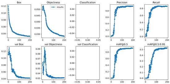
Figure 7.
Performance indicators of model training, including bounding box regression loss (Box), objectness loss (Objectness), classification loss (Classification), Precision, Recall, and mean average precision (mAP@0.5: IoU = 0.5, mAP@0.5:0.95: IoU ). val denotes the corresponding result on the validation set.
5.2. Evaluation Indicators
In this paper, we choose the inference time of the model at as a metric for detection speed, use mAP to evaluate the detection performance of the model, and adopt Mean Intersection over Union (MIoU), Mean Pixel Accuracy (MPA), and Accuracy to evaluate the segmentation performance. The metrics are defined as follows:
where C represents the number of target categories ( in this paper), denotes the number of IoU thresholds, k denotes the IoU threshold, denotes the precision under threshold, denotes the recall rate under threshold; denotes the number of pixels correctly predicted as water; refers to the number of pixels incorrectly predicted as nonwater; denotes the number of pixels incorrectly predicted as water; denotes the number of pixels correctly predicted as nonwater; and denotes the number of categories of pixels ( in this paper).
5.3. Parameter Analysis
In the cloud, we optimize semantic segmentation and object detection by joint training with the loss function defined in Equation (14). is a parameter that controls the weight of the segmentation loss. To explore the effect of this parameter on segmentation and detection, we perform a parameter sensitivity analysis on . The specific results of the experiment are shown in Table 1. The effect of on the evaluation metrics of segmentation and detection is not significant. In this paper, we choose to set the initial value of the segmentation loss weight to a high value of 0.9 at the beginning of the training, and gradually reduce this weight to 0.5 as the training progresses. Such a strategy ensures high-quality segmentation results while ensuring that the detection achieves a high mAP.

Table 1.
Sensitivity analysis of the parameter in the loss function.
5.4. Analysis of the Calculation Amount
In this paper, we perform object detection based on the corresponding mask constructed in the cloud. Before the detection task, the mask image is transmitted from the cloud to the front end, and the masked part enters the object detection convolutional network without generating any anchor frames or performing the corresponding subsequent computations.
Assuming that the detection network has a fixed amount of computation for each region of the image, it is assumed that the reduced amount of computation is related to the proportion of mask in the original image. It can be expressed by Equation (22).
where is the calculation amount required for network postprocessing after adding the Mask module and Anchor Head module, k is the percentage of the mask in the original image, and is the calculation amount required for all grids in the network. Let be the calculation amount required for network postprocessing of the original image.
The above scenario is ideal without considering the network latency between the front end and the cloud. In practical applications, network latency is an unavoidable problem. The network latency will affect the effect of the calculation reduction of our framework. Therefore, we update the Equation (22) to Equation (23).
where is the average network latency time in milliseconds, and is the average MFLOPS (Million Floating-point Operations per Second) of the CPU/GPU. is usually a very small value. These variables need to be obtained through statistics of practical applications.
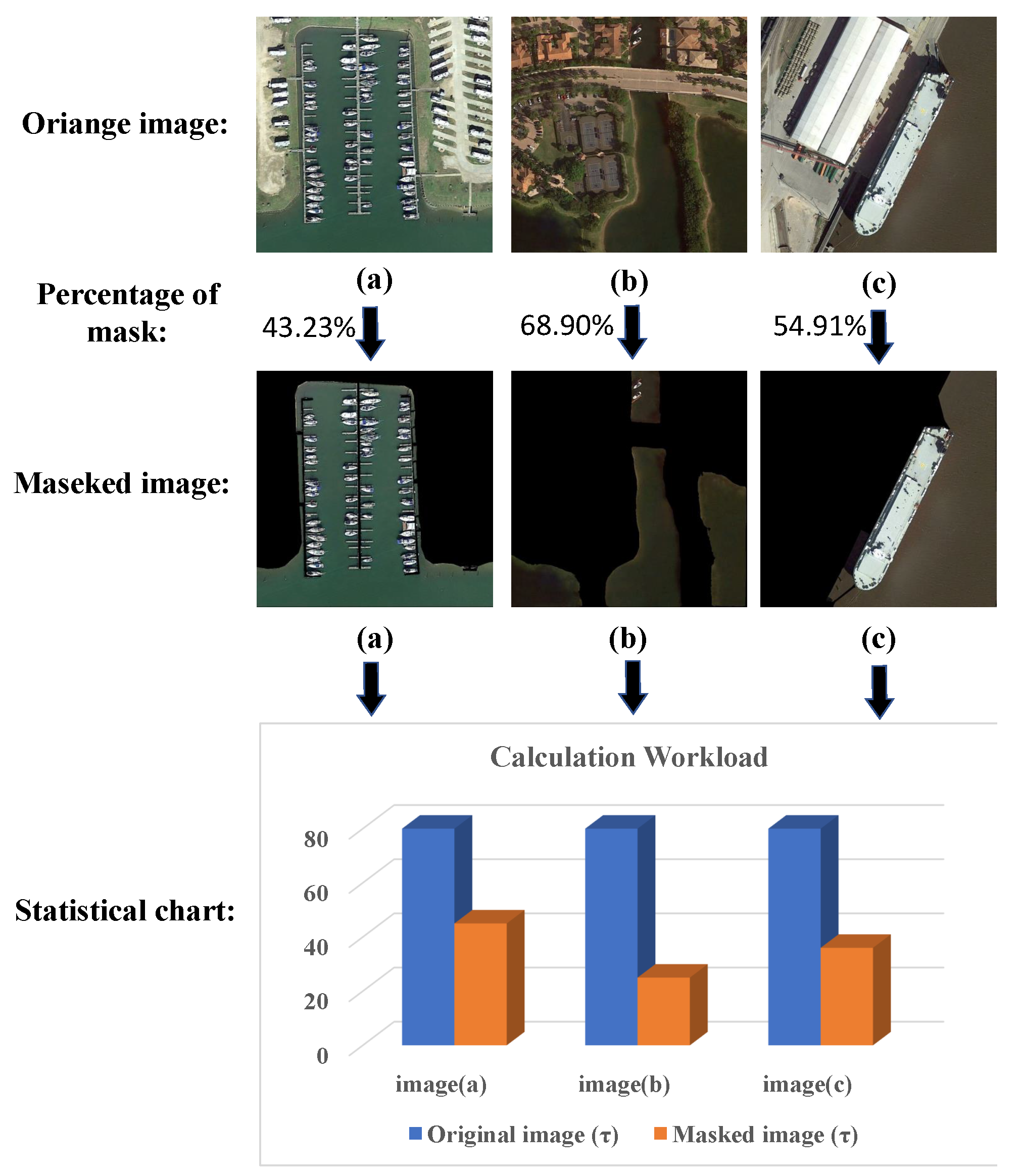
As shown in Figure 8, we take three remote sensing images in the dataset as an example. After these images go through the detection network, each image is divided into an grid. After adding the mask, the area where our network has to perform computation is significantly reduced, and no anchor frame is generated within the mask. Compared with the detection without masked features, our solution reduces the computational effort for the generation of anchor frames and the subsequent computation of the masked portion.
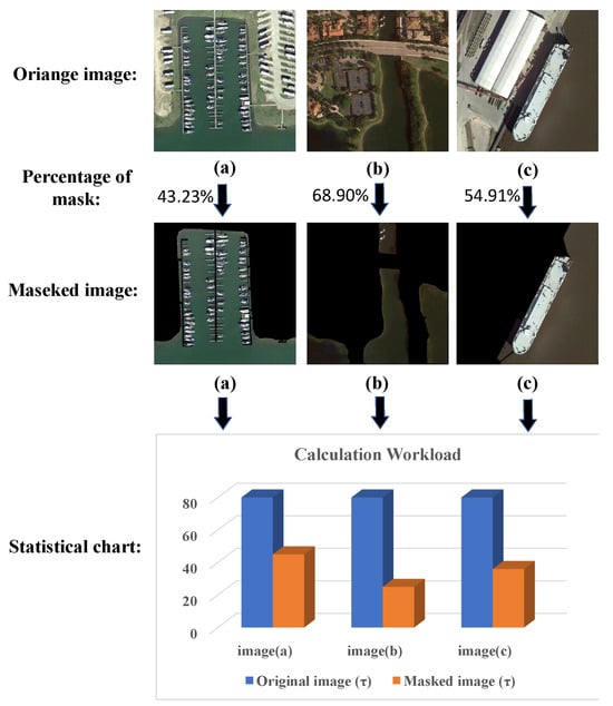
Figure 8.
Schematic diagram of mask operation and calculation reduction statistics. (a–c) are three remote sensing images in the dataset. The computation is reduced by adding a mask to the original image and not computing on the nonwater part.
5.5. Comparison with Other Detection Models
To analyze the ship detection performance of our proposed model, we compare the proposed object detection model with YOLOv3-tiny [44], YOLOv4s-tiny [45], YOLOv5s, YOLOv6s [46], YOLOv7-tiny [35], YOLOV8s, RT-DETR-R18 [47], and YOLOv5-ODConv-NeXt [48]. We use mAP, Parameters, Weight file size, and Giga Floating-point Operations Per Second (GFLOPs) as evaluation metrics. The comparison results are shown in Table 2. By jointly optimizing semantic segmentation and object detection, our detection model improves ship detection accuracy and performs well in terms of the number of parameters, weight file size, GFLOPs, and Speed. Our detection model achieves 92.4% accuracy. Compared with YOLOv3-tiny, YOLOv4-tiny, YOLOv5s, YOLOv6s, YOLOv7-tiny, YOLOv8s, RT-DETR-R18, and YOLOv5-ODConvNeXt, our model’s accuracy is 21.7%, 26.2%, 3.7%, and 13.3% higher, respectively, 2.9%, 2.3%, 14.7% and 0.4%. In terms of the number of parameters, our detection model has fewer parameters than other models: 30.2% fewer than YOLOv3-tiny, 1.6% fewer than YOLOv4-tiny, 14.3% fewer than YOLOv5s, 67.6% fewer than YOLOv6s, 45.9% fewer than YOLOv8s, 70% fewer than RT-DETR-R18, and 14.3% fewer than YOLOv5-ODConvNeXt. In terms of weight file size, the weight file size of our detection model is 30.9%, 1.1%, and 15.5% smaller than YOLOv3-tiny, YOLOv4-tiny, YOLOv5s, YOLOv6s, YOLOv7tiny, YOLOv8s, RT-DETR-R18, and YOLOv5-ODConvNeXt, respectively, 70.3%, 1.3%, 64.2%, 70.3%, and 15.2%. In terms of GFLOPs, our detection model has 24.8%, 41.2%, 38.6%, 78.8%, 25.4%, 65.8%, 83.8%, and 34.5% lower GFLOPs compared to YOLOv3-tiny, YOLOv4-tiny, YOLOv5s, YOLOv6s, YOLOv7-tiny, YOLOv8s, RT-DETR-R18, and YOLOv5-ODConvNeXt, respectively. The experiments show that our object detection model achieves lightweight while maintaining high accuracy.
Table 2.
Performance metrics of our object detection model. Our proposed method is compared with YOLOv3-tiny, YOLOv4-tiny, YOLOv5s, YOLOv6s, YOLOv7-tiny, YOLOv8s, RT-DETR-R18, YOLOv5-ODConvNeXt. The bold indicates the best result in each column, and the underline indicates the second-best result in each column.
5.6. Ablation Experiment
In this section, we perform the ablation experiments, which include postprocessing, semantic segmentation, and detection module.
5.6.1. Postprocessing
We compare different postprocessing methods, including NMS, Soft NMS [49], DIoU NMS [50], and the Confluence algorithm. Confluence algorithm determines the optimal box by identifying the box that intersects the most with other bounding boxes. It is more robust when dealing with densely distributed and small targets. Due to this feature, it shows better performance than other postprocessing methods. The comparison of detection results is shown in Table 3.
Table 3.
The ablation experiment results for different postprocessing methods. Bold indicates the best result in each column, and underline indicates the second-best result in each column.
5.6.2. Segmentation Module
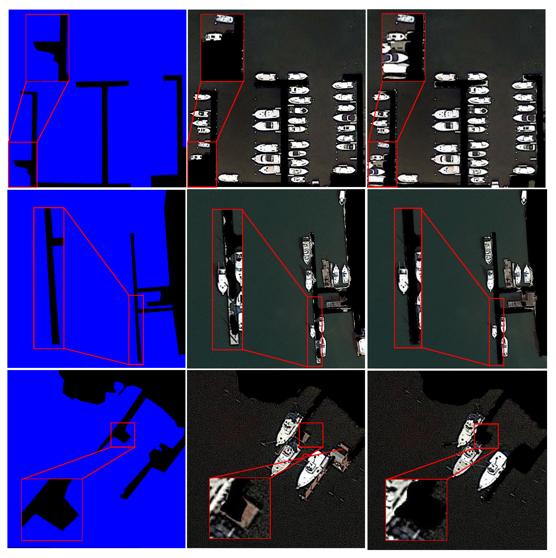
We conduct ablation experiments to explore the effect of joint optimization on the performance of semantic segmentation. According to Table 4, it can be seen that joint optimization will improve the performance of semantic segmentation. MIoU, MPA, and Accuracy of our model are 1%, 0.7%, and 0.5% higher than that of the segmentation-only model, respectively. Some segmentation results on the validation dataset are shown in Figure 9 to visualize the improvement. Our model can achieve more accurate segmentation results, especially preserving the ship target information.
Table 4.
The ablation experiment results for joint optimization of segmentation module. Bold indicates the best result in each column.
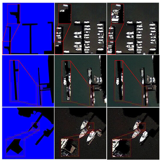
Figure 9.
Segmentation results of different models. The first column shows the segmentation results of the segmentation-only model, the second column shows the results of the joint optimization model, and the third column shows the ground truths. The red rectangle shows a partially enlarged detail of the image.
5.6.3. Detection Module
To quickly and accurately detect ship objects in remote sensing images, we design a segmentation and detection joint optimization network and use the Confluence algorithm, CA module, -IoU loss function, Mask module, and Anchor Head module to improve the YOLO model. A series of ablation experiments are conducted on the validation dataset to analyze which improvement plays a more critical role in improving detection performance. The results are shown in Table 5. When the joint optimization of semantic segmentation and object detection is used, mAP@0.5 and mAP@0.95 of the detection model increase by 0.9% and 1.6%, respectively, compared with the object-detection-only model. After introducing the Confluence algorithm, -IoU loss, CA module, Mask module, and Anchor Head module, mAP@0.5 and mAP@0.95 of the detection model reach up to 92.4% and 52.9%, which increase by 2.7% and 6.9%, respectively, compared with the object-detection-only model.
Table 5.
The ablation experiment results for the detection module. Bold indicates the best result in each column, and underline indicates the second-best result in each column.
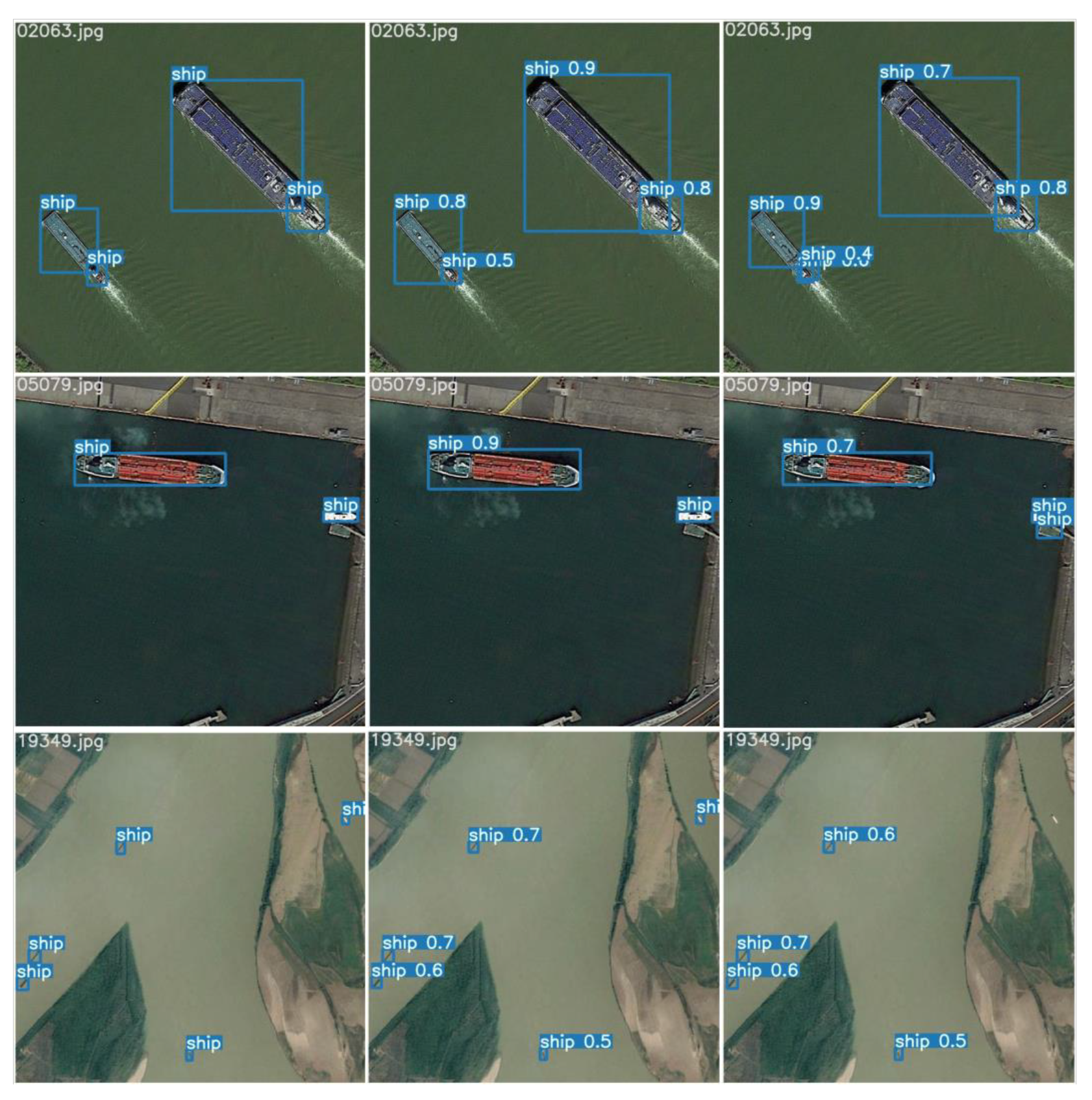
In this paper, we use the -IoU loss function defined in Equation (11). is a hyperparameter. To further illustrate the detection effect of different values of , we visualize some detection cases in Figure 10. When , both large and small ships can be accurately detected. When , there will be bounding box overlap (first and second rows in Figure 10) and missed detection (third row in Figure 10) problems for small ships. The increase in causes the detection model to be overly sensitive to small targets, resulting in bounding box overlaps for small ships.
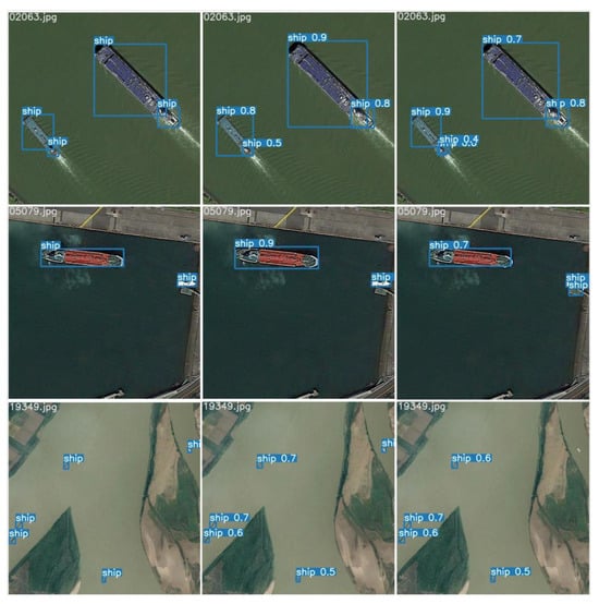
Figure 10.
Sensitivity analysis of in the loss function. The first column shows the detection results when , the second column shows the detection results when , and the third column shows the ground truths.
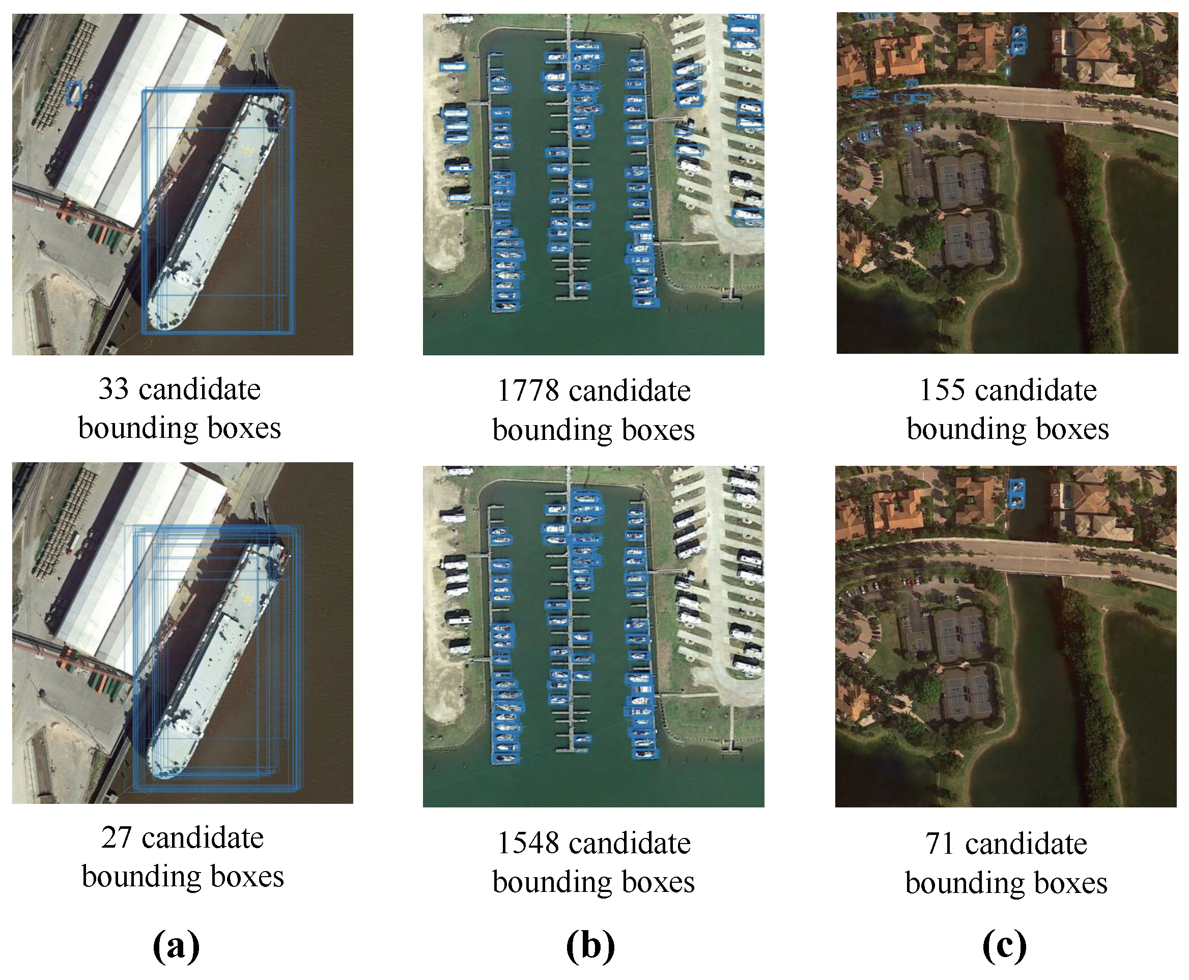
In the device–cloud collaboration architecture, the role of the cloud is mainly to store the semantic mask images and transmit the corresponding mask images to the front end based on the geolocation information sent by the front end. In this process, the computational burden of the cloud is almost negligible. Although the complete image data still need to be input into the network at the front end, we design the Mask module and Anchor Head module to use the mask images received from the cloud to exclude the nonwater portion and reduce the number of candidate bounding boxes, thus reducing the computational burden on the front end. To validate the effectiveness of our approach, we show three visualization examples of candidate bounding boxes output by the model before postprocessing in Figure 11. For these cases, the number of candidate bounding boxes is reduced by 18.2%, 12.9%, and 54.2%, respectively. We further analyze the memory and time consumption of the postprocessing procedure. As shown in Table 6, by applying mask images to the network, our network reduces the processing time by 0.1ms without increasing the peak memory and total memory footprint, which is essential when real-time ship detection is implemented on a front-end device with limited computation resources.
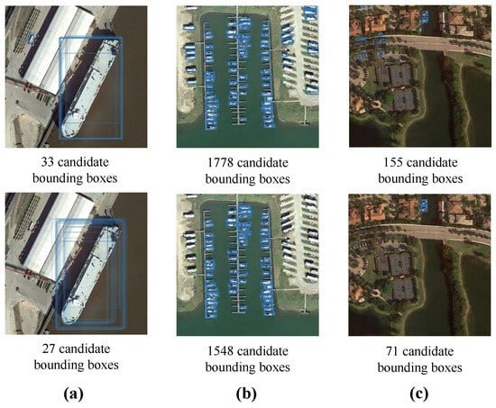
Figure 11.
Candidate bounding box visualization generated by YOLO model before NMS (first row) and candidate bounding box visualization generated by our model before NMS (second row). (a–c) are three remote sensing images in the dataset.
Table 6.
Comparison results of postprocessing time consumption, peak memory, and average memory usage.
5.7. Efficiency Analysis
As shown in Table 7, we analyze the efficiency of semantic segmentation, network transmission, and detection network in the device–cloud collaborative framework, where Cloud denotes the time required for semantic segmentation in the cloud, Transmission denotes the time required to transmit the mask image from the cloud to the front end, and End denotes the time required for ship detection in the front end. First, we verify the effect of the improvement on the detection speed by ablation experiments and then compare the performance of other models in terms of ship detection speed.
Table 7.
Device–Cloud Collaboration Efficiency Analysis Experiment (ablation of the model and comparison with other models). Bold indicates the best result in each column, and underline indicates the second-best result in each column.
The time required for semantic segmentation in the cloud is about 2.1 ms. It can be assumed that the size of the segmented mask image is 10 KB and the 5G bandwidth is 500 Mbit/s. The transmission time of a mask image is about 0.16 ms without considering the network latency and other interferences. As shown in Table 7, the addition of the MASK module reduces the calculation of nonwater areas and reduces the average ship detection speed from 5.4 ms to 3.1 ms, which is a 42.6% improvement in detection speed. Compared with other models, the inference speed of YOLOv3-tiny is the fastest, but there is a large sacrifice in accuracy, which makes it difficult to meet the requirements of ship detection tasks. Compared with YOLOv4-tiny, YOLOV5s, YOLOv6s, YOLOv7-tiny, YOLOv8s, RT-DETR-R18, and YOLOv5-ODConvNeXt, our method has faster inference speed.
For our device–cloud collaborative approach, the ship detection process does not directly perform the inference of the semantic segmentation network. The cloud is responsible for receiving the position information sent by the front-end device and returning the corresponding mask image stored in the cloud to the front end. Therefore, the cloud’s processing time can be negligible. Through this device–cloud collaborative approach, not only the speed of ship detection is improved but also the accuracy of ship detection is ensured.
5.8. Attention Visualization Analysis
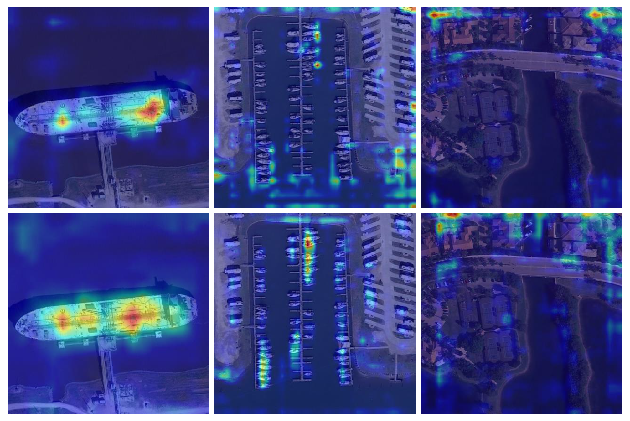
In order to visualize the specific effect of the CA attention mechanism on the detection process, we select three images in the dataset and perform a heatmap visualization of the first detection layer, as shown in Figure 12. Specifically, the attention area of the original model is not enough, and the correlation between the thermal distribution and the ship’s geometric distribution is weak. After adding the CA module, our model significantly improves this shortcoming with a more concentrated heat distribution and a stronger correlation between the thermal distribution and the ship’s geometric distribution. This indicates that the CA attention mechanism can effectively enhance the model’s attention to the ship region and improve detection accuracy.

Figure 12.
Visualization of attention. The first row shows the heatmap visualization results without adding the CA attention mechanism, and the second row shows the heatmap visualization results after adding the CA attention mechanism. The blue area represents the part where the model pays less attention, while the yellow and red areas represent the parts where the model pays more attention. Specifically, the red area shows higher attention relative to the yellow area. This color difference reflects the attention level and priority of the model when processing the visual input.
5.9. Visualization of Results
5.9.1. Semantic Segmentation
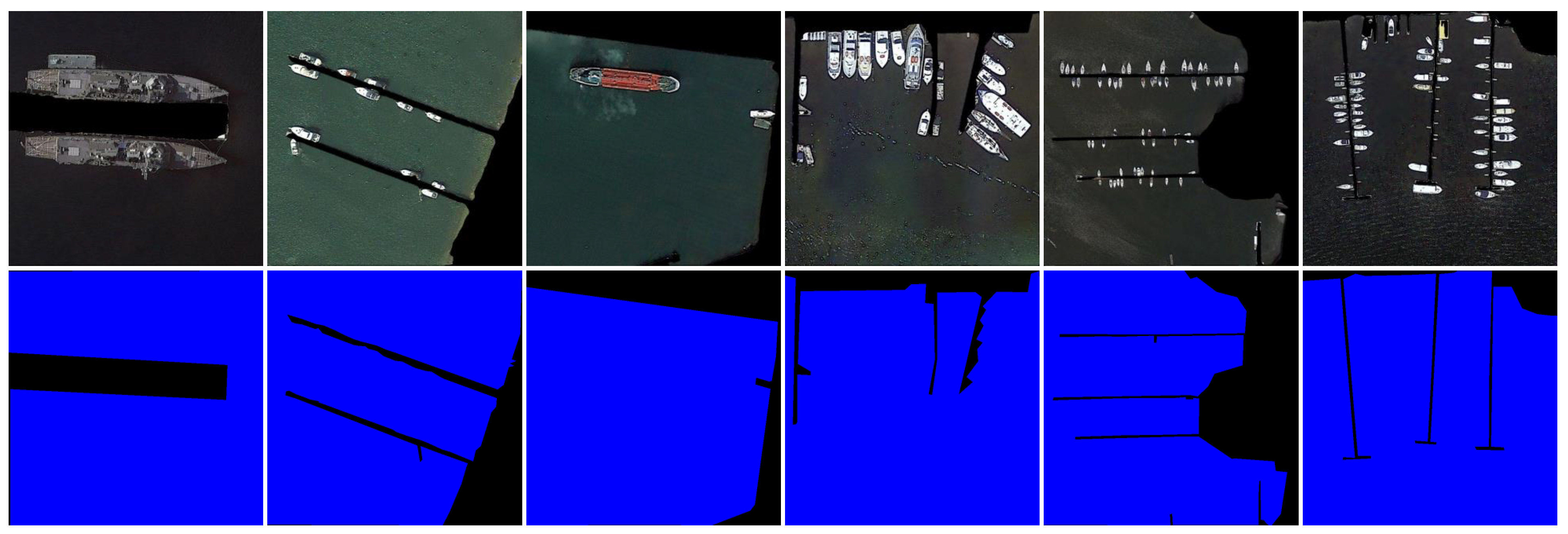
We deploy the segmentation module in the cloud and utilize the weight file obtained through joint optimization to perform the segmentation task. After completing this task, we store the semantic segmentation results in the cloud for subsequent calculations. Some segmentation results and their corresponding ground truths are shown in Figure 13. It can be seen that our segmentation model can effectively segment water and nonwater areas.
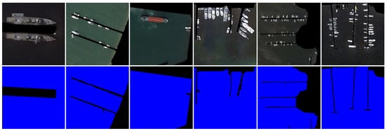
Figure 13.
Segmentation results (first row) and ground truths (second row) visualization.
5.9.2. Object Detection
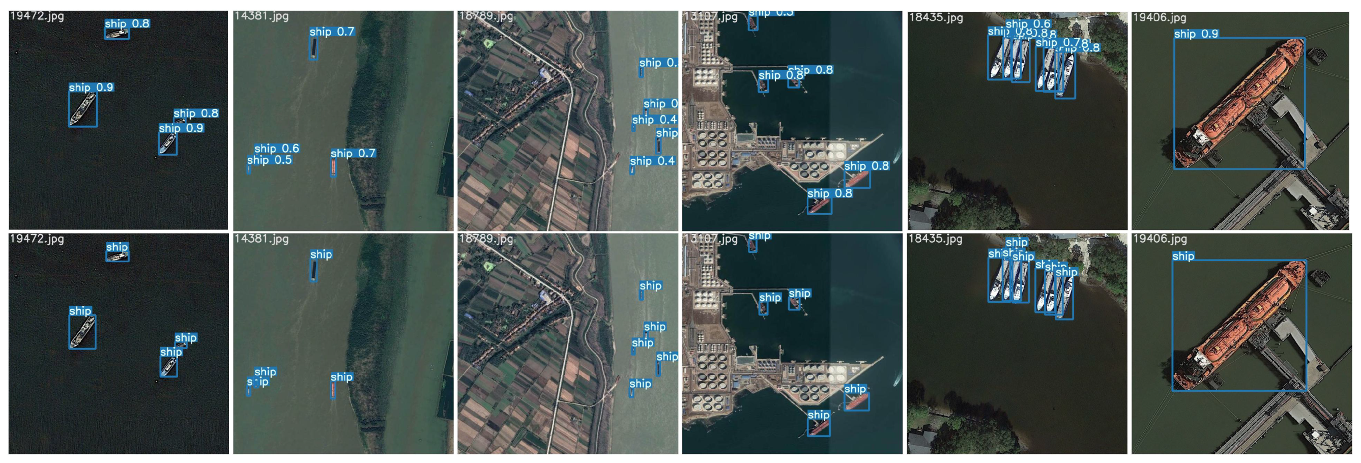
We deploy the object detection module in the front end and utilize the weight file obtained through joint optimization to perform the ship detection task. The corresponding semantic segmentation results in the cloud will be used for detection. Some ship detection results and their corresponding ground truths are shown in Figure 14. It can be seen that our model can accurately detect ships in remote sensing images.
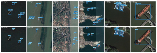
Figure 14.
Ship detection results (first row) and ground truths (second row) visualization.
6. Conclusions
In order to achieve fast and accurate detection of ship targets in remote sensing images under the environment of limited front-end computing power, this paper proposes an efficient ship detection model based on device–cloud collaboration. The model improves the overall performance of the system by jointly optimizing semantic segmentation and object detection. The ship targets in remote sensing images are small, and the image background is complex. We introduce the coordinate attention mechanism, -IoU loss, and Confluence algorithm to enhance the detection accuracy of small targets. The constructed SD-Net outperforms the current detection methods in terms of mAP, Params, and GFLOPs. By utilizing the mask image sent by the cloud, the calculation required for detection in nonwater areas is reduced, reducing the detection time from 5.4 ms to 3.1 ms (improving the detection speed by 42.6%). This is particularly suitable for front-end devices (UAV) with limited computing and power resources. It not only maintains high detection accuracy but also reduces the consumption of computing resources, thereby increasing the endurance of UAVs.
The device–cloud collaboration method is limited by network bandwidth to a certain extent. To reduce the impact of network bandwidth, we will consider using spike neural networks to further reduce the amount of calculations and combine knowledge distillation techniques to further improve the reasoning speed. With the development of information transmission technology, we will also explore the use of edge computing to optimize the model computing architecture. For the changeable climate environment at sea, we will also explore the ship detection methods under different weather conditions in the future.
Author Contributions
Conceptualization, T.L. and Y.Y.; methodology, T.L., Y.Y. and Z.L.; software, T.L. and Y.Y.; validation, T.L., Y.Y. and Z.L.; formal analysis, Y.H. and X.Z.; investigation, T.L. and Y.Y.; resources, Z.L.; data curation, Y.Y.; writing—original draft preparation, T.L. and Y.Y.; writing—review and editing, F.W., M.S. and H.W.; visualization, T.L. and Y.Y.; supervision, M.S. and H.W.; project administration, T.L. and Z.L.; funding acquisition, T.L. and Z.L. All authors have read and agreed to the published version of the manuscript.
Funding
This work was supported in part by the National Natural Science Foundation of China under Grant 52071201, Grant 52301420, and Grant 52331012, in part by the Science and Technology Commission of Shanghai Municipality (STCSM) Capacity Building Project of Local Universities under Grant 23010502200, in part by the Special Funding for the Development of Science and Technology of Shanghai Ocean University under Grant A2-2006-21-200207, in part by the Open Fund of Key Laboratory of High-Performance Ship Technology (Wuhan University of Technology), Ministry of Education under Grant GXNC23052801, in part by the Open Project Program of the State Key Laboratory of CAD&CG (Zhejiang University) under Grant A2326, and in part by Fund from State Key Laboratory of Maritime Technology and Safety. (Corresponding author: Zhengling Lei).
Institutional Review Board Statement
Not applicable.
Informed Consent Statement
Not applicable.
Data Availability Statement
The data that support the findings of this study are available from the corresponding author, [Z.L. Lei], upon reasonable request.
Conflicts of Interest
The authors declare no conflicts of interest.
References
- Zhenbo, B.; Shiyou, Z.; Hua, Y.; Yuanhong, W. Survey of Ship Detection in Video Surveillance Based on Shallow Machine Learning. J. Syst. Simul. 2021, 33, 16. [Google Scholar]
- Dudczyk, J.; Rybak, Ł. Application of data particle geometrical divide algorithms in the process of radar signal recognition. Sensors 2023, 23, 8183. [Google Scholar] [CrossRef]
- Dudczyk, J.; Kawalec, A. Specific emitter identification based on graphical representation of the distribution of radar signal parameters. Bull. Pol. Acad. Sci. Tech. Sci. 2015, 63, 391–396. [Google Scholar] [CrossRef]
- Dudczyk, J. Radar emission sources identification based on hierarchical agglomerative clustering for large data sets. J. Sens. 2016, 2016, 1879327. [Google Scholar] [CrossRef]
- Chen, X.; Wu, H.; Han, B.; Liu, W.; Montewka, J.; Liu, R.W. Orientation-aware ship detection via a rotation feature decoupling supported deep learning approach. Eng. Appl. Artif. Intell. 2023, 125, 106686. [Google Scholar] [CrossRef]
- Chen, X.; Wei, C.; Yang, Y.; Luo, L.; Biancardo, S.A.; Mei, X. Personnel trajectory extraction from port-like videos under varied rainy interferences. IEEE Trans. Intell. Transp. Syst. 2024, 25, 6567–6579. [Google Scholar] [CrossRef]
- Carion, N.; Massa, F.; Synnaeve, G.; Usunier, N.; Kirillov, A.; Zagoruyko, S. End-to-end object detection with transformers. In Proceedings of the European Conference on Computer Vision; Springer: Berlin/Heidelberg, Germany, 2020; pp. 213–229. [Google Scholar]
- Dai, X.; Chen, Y.; Yang, J.; Zhang, P.; Yuan, L.; Zhang, L. Dynamic detr: End-to-end object detection with dynamic attention. In Proceedings of the IEEE/CVF International Conference on Computer Vision, Montreal, BC, Canada, 11–17 October 2021; pp. 2988–2997. [Google Scholar]
- Li, J.; Tian, P.; Song, R.; Xu, H.; Li, Y.; Du, Q. PCViT: A Pyramid Convolutional Vision Transformer Detector for Object Detection in Remote Sensing Imagery. IEEE Trans. Geosci. Remote Sens. 2024, 62, 5608115. [Google Scholar] [CrossRef]
- Yan, R.; Yan, L.; Geng, G.; Cao, Y.; Zhou, P.; Meng, Y. ASNet: Adaptive Semantic Network Based on Transformer-CNN for Salient Object Detection in Optical Remote Sensing Images. IEEE Trans. Geosci. Remote Sens. 2024, 62, 5608716. [Google Scholar] [CrossRef]
- Zhao, T.; Wang, Y.; Li, Z.; Gao, Y.; Chen, C.; Feng, H.; Zhao, Z. Ship Detection with Deep Learning in Optical Remote-Sensing Images: A Survey of Challenges and Advances. Remote Sens. 2024, 16, 1145. [Google Scholar] [CrossRef]
- Long, J.; Shelhamer, E.; Darrell, T. Fully convolutional networks for semantic segmentation. In Proceedings of the IEEE Conference on Computer Vision and Pattern Recognition, Boston, MA, USA, 7–12 June 2015; pp. 3431–3440. [Google Scholar]
- Shen, Q.; Gao, C. Research on Semantic Segmentation of Natural Landform Based on Edge Detection Module. J. Syst. Simul. 2022, 34, 293–302. [Google Scholar]
- Li, Y.; Chen, W.; Huang, X.; Gao, Z.; Li, S.; He, T.; Zhang, Y. MFVNet: A deep adaptive fusion network with multiple field-of-views for remote sensing image semantic segmentation. Sci. China Inf. Sci. 2023, 66, 140305. [Google Scholar] [CrossRef]
- Cai, Y.; Fan, L.; Fang, Y. SBSS: Stacking-Based Semantic Segmentation Framework for Very High-Resolution Remote Sensing Image. IEEE Trans. Geosci. Remote Sens. 2023, 61, 1–14. [Google Scholar] [CrossRef]
- Saralioglu, E.; Gungor, O. Semantic segmentation of land cover from high resolution multispectral satellite images by spectral-spatial convolutional neural network. Geocarto Int. 2022, 37, 657–677. [Google Scholar] [CrossRef]
- Wu, H.; Huang, P.; Zhang, M.; Tang, W.; Yu, X. CMTFNet: CNN and Multiscale Transformer Fusion Network for Remote Sensing Image Semantic Segmentation. IEEE Trans. Geosci. Remote Sens. 2023, 61, 2004612. [Google Scholar] [CrossRef]
- Xiao, T.; Liu, Y.; Huang, Y.; Li, M.; Yang, G. Enhancing Multiscale Representations with Transformer for Remote Sensing Image Semantic Segmentation. IEEE Trans. Geosci. Remote Sens. 2023, 61, 1–16. [Google Scholar] [CrossRef]
- He, X.; Zhou, Y.; Zhao, J.; Zhang, D.; Yao, R.; Xue, Y. Swin transformer embedding UNet for remote sensing image semantic segmentation. IEEE Trans. Geosci. Remote Sens. 2022, 60, 1–15. [Google Scholar] [CrossRef]
- Li, L.; Jiang, L.; Zhang, J.; Wang, S.; Chen, F. A complete YOLO-based ship detection method for thermal infrared remote sensing images under complex backgrounds. Remote Sens. 2022, 14, 1534. [Google Scholar] [CrossRef]
- You, Y.; Cao, J.; Zhang, Y.; Liu, F.; Zhou, W. Nearshore ship detection on high-resolution remote sensing image via scene-mask R-CNN. IEEE Access 2019, 7, 128431–128444. [Google Scholar] [CrossRef]
- Tian, Y.; Liu, J.; Zhu, S.; Xu, F.; Bai, G.; Liu, C. Ship Detection in Visible Remote Sensing Image Based on Saliency Extraction and Modified Channel Features. Remote Sens. 2022, 14, 3347. [Google Scholar] [CrossRef]
- Liu, T.; Jia, Z.; Lei, Z.; Zhang, X.; Huo, Y. Unsupervised depth estimation for ship target based on single view UAV image. Int. J. Remote Sens. 2022, 43, 3216–3235. [Google Scholar] [CrossRef]
- Xu, X.; Zhang, X.; Zhang, T. Lite-yolov5: A lightweight deep learning detector for on-board ship detection in large-scene sentinel-1 sar images. Remote Sens. 2022, 14, 1018. [Google Scholar] [CrossRef]
- Tian, Y.; Wang, X.; Zhu, S.; Xu, F.; Liu, J. LMSD-Net: A Lightweight and High-Performance Ship Detection Network for Optical Remote Sensing Images. Remote Sens. 2023, 15, 4358. [Google Scholar] [CrossRef]
- Peng, G.; Yang, Z.; Wang, S.; Zhou, Y. AMFLW-YOLO: A Lightweight Network for Remote Sensing Image Detection Based on Attention Mechanism and Multi-scale Feature Fusion. IEEE Trans. Geosci. Remote Sens. 2023, 61, 4600916. [Google Scholar] [CrossRef]
- Liu, T.; Zhang, Z.; Lei, Z.; Huo, Y.; Wang, S.; Zhao, J.; Zhang, J.; Jin, X.; Zhang, X. An approach to ship target detection based on combined optimization model of dehazing and detection. Eng. Appl. Artif. Intell. 2024, 127, 107332. [Google Scholar] [CrossRef]
- Liu, L.; Chen, H.; Xu, Z. SPMOO: A Multi-Objective Offloading Algorithm for Dependent Tasks in IoT Cloud-Edge-End Collaboration. Information 2022, 13, 75. [Google Scholar] [CrossRef]
- Liu, F.; Huang, J.; Wang, X. Joint Task Offloading and Resource Allocation for Device-Edge-Cloud Collaboration with Subtask Dependencies. IEEE Trans. Cloud Comput. 2023, 11, 3027–3039. [Google Scholar] [CrossRef]
- Zhuang, Y.; Zheng, Z.; Shao, Y.; Li, B.; Wu, F.; Chen, G. ECLM: Efficient Edge-Cloud Collaborative Learning with Continuous Environment Adaptation. arXiv 2023, arXiv:2311.11083. [Google Scholar]
- Wang, Y.; Xu, R.; Zhou, C.; Kang, X.; Chen, Z. Digital twin and cloud-side-end collaboration for intelligent battery management system. J. Manuf. Syst. 2022, 62, 124–134. [Google Scholar] [CrossRef]
- Zhang, K.; Huang, W.; Hou, X.; Xu, J.; Su, R.; Xu, H. A fault diagnosis and visualization method for high-speed train based on edge and cloud collaboration. Appl. Sci. 2021, 11, 1251. [Google Scholar] [CrossRef]
- Tan, G.; Li, C.; Zhan, Z. Adaptive Scheduling Algorithm for Object Detection and Tracking Based on Device-Cloud Collaboration. J. South China Univ. Technol. Nat. Sci. Ed. 2021, 49. [Google Scholar]
- Chen, L.C.; Zhu, Y.; Papandreou, G.; Schroff, F.; Adam, H. Encoder-decoder with atrous separable convolution for semantic image segmentation. In Proceedings of the European Conference on Computer Vision (ECCV), Munich, Germany, 8–14 September 2018; pp. 801–818. [Google Scholar]
- Wang, C.Y.; Bochkovskiy, A.; Liao, H.Y.M. YOLOv7: Trainable bag-of-freebies sets new state-of-the-art for real-time object detectors. In Proceedings of the IEEE/CVF Conference on Computer Vision and Pattern Recognition, Vancouver, BC, Canada, 17–24 June 2023; pp. 7464–7475. [Google Scholar]
- Chen, L.C.; Papandreou, G.; Schroff, F.; Adam, H. Rethinking atrous convolution for semantic image segmentation. arXiv 2017, arXiv:1706.05587. [Google Scholar]
- Hou, Q.; Zhou, D.; Feng, J. Coordinate attention for efficient mobile network design. In Proceedings of the IEEE/CVF Conference on Computer Vision and Pattern Recognition, Nashville, TN, USA, 19–25 June 2021; pp. 13713–13722. [Google Scholar]
- Neubeck, A.; Van Gool, L. Efficient non-maximum suppression. In Proceedings of the 18th International Conference on Pattern Recognition (ICPR’06), Hong Kong, China, 20–24 August 2006; Volume 3, pp. 850–855. [Google Scholar]
- Shepley, A.J.; Falzon, G.; Kwan, P.; Brankovic, L. Confluence: A robust non-IoU alternative to non-maxima suppression in object detection. IEEE Trans. Pattern Anal. Mach. Intell. 2023, 45, 11561–11574. [Google Scholar] [CrossRef]
- He, J.; Erfani, S.; Ma, X.; Bailey, J.; Chi, Y.; Hua, X.S. α-IoU: A family of power intersection over union losses for bounding box regression. Adv. Neural Inf. Process. Syst. 2021, 34, 20230–20242. [Google Scholar]
- Li, K.; Wan, G.; Cheng, G.; Meng, L.; Han, J. Object detection in optical remote sensing images: A survey and a new benchmark. ISPRS J. Photogramm. Remote Sens. 2020, 159, 296–307. [Google Scholar] [CrossRef]
- Xia, G.S.; Bai, X.; Ding, J.; Zhu, Z.; Belongie, S.; Luo, J.; Datcu, M.; Pelillo, M.; Zhang, L. DOTA: A large-scale dataset for object detection in aerial images. In Proceedings of the IEEE Conference on Computer Vision and Pattern Recognition, Salt Lake City, UT, USA, 18–23 June 2018; pp. 3974–3983. [Google Scholar]
- Zou, Z.; Shi, Z. Random access memories: A new paradigm for target detection in high resolution aerial remote sensing images. IEEE Trans. Image Process. 2017, 27, 1100–1111. [Google Scholar] [CrossRef]
- Redmon, J.; Farhadi, A. Yolov3: An incremental improvement. arXiv 2018, arXiv:1804.02767. [Google Scholar]
- Bochkovskiy, A.; Wang, C.Y.; Liao, H.Y.M. Yolov4: Optimal speed and accuracy of object detection. arXiv 2020, arXiv:2004.10934. [Google Scholar]
- Li, C.; Li, L.; Jiang, H.; Weng, K.; Geng, Y.; Li, L.; Ke, Z.; Li, Q.; Cheng, M.; Nie, W.; et al. YOLOv6: A single-stage object detection framework for industrial applications. arXiv 2022, arXiv:2209.02976. [Google Scholar]
- Lv, W.; Xu, S.; Zhao, Y.; Wang, G.; Wei, J.; Cui, C.; Du, Y.; Dang, Q.; Liu, Y. Detrs beat yolos on real-time object detection. arXiv 2023, arXiv:2304.08069. [Google Scholar]
- Cheng, S.; Zhu, Y.; Wu, S. Deep learning based efficient ship detection from drone-captured images for maritime surveillance. Ocean Eng. 2023, 285, 115440. [Google Scholar] [CrossRef]
- Bodla, N.; Singh, B.; Chellappa, R.; Davis, L.S. Soft-NMS–improving object detection with one line of code. In Proceedings of the IEEE International Conference on Computer Vision, Venice, Italy, 22–29 October 2017; pp. 5561–5569. [Google Scholar]
- Zheng, Z.; Wang, P.; Liu, W.; Li, J.; Ye, R.; Ren, D. Distance-IoU loss: Faster and better learning for bounding box regression. In Proceedings of the AAAI Conference on Artificial Intelligence, New York, NY, USA, 7–12 February 2020; Volume 34, pp. 12993–13000. [Google Scholar]
Disclaimer/Publisher’s Note: The statements, opinions and data contained in all publications are solely those of the individual author(s) and contributor(s) and not of MDPI and/or the editor(s). MDPI and/or the editor(s) disclaim responsibility for any injury to people or property resulting from any ideas, methods, instructions or products referred to in the content. |
© 2024 by the authors. Licensee MDPI, Basel, Switzerland. This article is an open access article distributed under the terms and conditions of the Creative Commons Attribution (CC BY) license (https://creativecommons.org/licenses/by/4.0/).