Article

Trajectory Tracking Control for an Underactuated AUV via Nonsingular Fast Terminal Sliding Mode Approach

School of Computer and Control Engineering, Yantai University, Yantai 264005, China
*
Author to whom correspondence should be addressed.
J. Mar. Sci. Eng. 2024, 12(8), 1442; https://doi.org/10.3390/jmse12081442
Submission received: 16 July 2024 / Revised: 7 August 2024 / Accepted: 10 August 2024 / Published: 21 August 2024
(This article belongs to the Section Ocean Engineering)

Abstract

:
This paper studies the trajectory tracking issue for an underactuated autonomous underwater vehicle (AUV) in the horizontal plane. The desired velocity–tracking error relationship (DVTER) is constructed according to the kinematics and kinetic equation, which means that the expected velocities are built so that the position tracking errors converge to 0. Moreover, the limitation of obtaining the expected velocity by directly differentiating the desired position values is avoided. Then, the nonsingular fast terminal sliding mode (TSM) controller is developed to ensure that the velocities converge to the designed expected values in finite time, and tracking speed is improved by comparing with the traditional nonsingular terminal sliding mode method. It turns out that the expected trajectory can be tracked by an underactuated AUV. Finally, the efficiency of the constructed control mechanism is confirmed by simulation results.

1. Introduction

AUVs are widely used in ocean exploration and ocean mapping [1,2,3,4,5,6,7]. Their precise and efficient trajectory tracking ability is important for accomplishing operational tasks. Only a set of functional rudders and a stern thruster are included in the equipment of a conventional AUV, which is a kind of underactuated system [8]. Owing to nonholonomic constraints of the underactuated AUV and the Brockett necessary condition, there is no smooth time-invariant state feedback control rule. Moreover, the underactuated AUV’s mathematical model has high nonlinear coupling, which makes trajectory tracking control a unique difficulty.
To tackle the above problem, many control techniques have been created in recent years, including backstepping methods [9,10], neural network (NN) control methods [11,12], and sliding mode control methods [13,14]. In [9], a tracking controller is designed for a torpedo-like underactuted AUV based on backstepping and time delay estimation. A backstepping controller is created using a virtual velocity error variable that is defined, successfully avoiding the singular value issue that arises with backstepping control laws [10]. Generally, the large computational burden problem cannot be addressed easily in the backstepping control design process. For NN control methods, a global adaptive NN control method is designed for the underactuated AUV [11]. An L2 gain robust controller is constructed on the basis of a fuzzy NN [12]. Moreover, a trajectory tracking control technique is developed for underactuated AUVs using contraction theory [15]. However, the convergence speed is not considered. Regarding with the sliding mode control methods, the speed jump issue in backstepping is resolved by an adaptive chattering free sliding mode controller [13]. To attain asymptotic convergence of trajectory tracking error, Taha Elmokadem et al. construct an integral sliding mode control technique [14].
Recently, terminal sliding mode (TSM) has received extensive research [16,17,18,19,20]. For example, reference [16] proposes a nonsingular terminal sliding mode controller (NTSMC) for rigid robotic arms. A guidance law is developed based on nonsingular TSM for target interception [17]. Feng Yong et al. delve deeper into the singularity problem of TSM and propose NTSMC for second-order, third-order, and higher-order systems [18]. Taha Elmokadem et al. employ TSM, fast TSM, and nonsingular TSM methods to design controllers for underactuated AUVs to achieve the goal of trajectory tracking [21]. However, when far from the equilibrium point, the terminal sliding mode controller (TSMC) and NTSMC converge quite slowly. When these methods are adopted, the trajectory tracking speed of the underactuated AUV will be affected. Moreover, the singularity problem of TSMC still needs to be further investigated. There is still some research space to achieve fast trajectory tracking using the theoretical framework of TSMC. Regarding the singularity problem, the nonsingular fast TSM approach is studied in [22]. However, velocity tracking error convergence cannot ensure position tracking error convergence. Also, the variables on the horizontal and vertical axes are combined into one variable. These may affect the precise trajectory tracking control.
Inspired by the above discussion, this paper aims to construct a novel kind of TSMC for an underactuated AUV. The major contributions are as follows:
(1) DVTER is built according to the kinematics equation and kinetic equation of an underactuated AUV, which reveals the relationship between expected velocities and position errors. Also, DVTER lays the foundation for subsequent controller design. Compared with [22], on the basis of the constructed DVTER, the velocity tracking error convergence can ensure the convergence of the position tracking error.
(2) A nonsingular fast TSM controller is built for an underactuated AUV, which gets around the fast TSM control technique’s singularity issue. Compared with the non-singular TSM [21], the limitation of slow convergence rate is overcome. Moreover, different from the method in [22], two sliding mode surfaces are constructed according to forward and backward velocity tracking error and lateral velocity tracking error, respectively. When constructing the controller based on the designed sliding surfaces, more adjustable parameters are introduced in the controller, which is more general and flexible.

2. Problem Formulation

When describing the motion of the AUV in space, it is necessary to establish an inertial coordinate {I} and a three-dimensional coordinate {B}, as shown in Figure 1.
The kinematic model is defined as follows for an underactuated AUV in the horizontal plane [23]:
x ˙ = u cos ψ v sin ψ
y ˙ = u sin ψ + v cos ψ
ψ ˙ = r                                                            
where u, v, and r are forward and backward, lateral, and yaw angular velocity described in {B}. ψ represents yaw angle described in {I}. x, y are coordinates of the AUV centroid, representing displacement of the AUV in the directions of the O I X and O I Y axes of {I}.
The dynamic equation is described as [23]:
u ˙ = M 1 ( X u u + a 23 v r + τ u )
v ˙ = M 2 ( Y v v + a 13 u r )
r ˙ = M 3 ( N r r + a 12 u v + τ r )
where M 1 = 1 / ( m X u ˙ ) , M 2 = 1 / ( m Y v ˙ ) , a 23 = m Y v ˙ , M 3 = 1 / ( I z N r ˙ ) , a 12 = Y v ˙ X u ˙ , a 13 = X u ˙ m . τ u , τ r are longitudinal thrust and yaw moment, respectively. m represents the mass of the underactuated AUV. I z represents the rotational inertia around the z-axis. X u , Y v , and N r represent the damping coefficient. The semi-empirical approach or hydrodynamic computation programs can be used to calculate the damping coefficients [24]. The damping coefficient in the x direction is caused by the viscous force acting on the frontal area of the vehicle body, including the propeller housings, and the skin frictional force acting on the wetted surface of the vehicle. Viscosity on the side projecting sections of the hull and the propeller housings is responsible for the damping coefficients in the y and z axes [25]. Also, the system’s damping is speed-sensitive [26]. X u ˙ , Y v ˙ , and N r ˙ are hydrodynamic additional mass. Since the trajectory tracking control of the AUV in the horizontal plane is the main topic of this work, it does not involve the ascent and descent actions. Thus, for the convenience of clear description, the underactuated AUV is assumed to be suspended, and its center of buoyancy coincides with its center of gravity.
To make the following analysis easier, the following lemma and theorem are given.
Lemma 1 ([27]).
The sliding surface has the following design:
σ = x + k 1 s i g n a 1 x + k 2 s i g n a 2 x ˙
The system states x and x ˙ are globally finite time stable and converge to equilibrium point ( x , x ˙ ) = ( 0 , 0 ) in time T n f on sliding mode surface σ = 0 , where
T n f = 0 x ( 0 ) k 2 1 / a 2 ( x + k 1 x a 1 ) 1 / a 2 d x = a 2 x ( 0 ) 1 1 / a 2 k 1 ( a 2 1 ) · F ( 1 a 2 , a 2 1 a 2 ( a 1 1 ) ; 1 + a 2 1 a 2 ( a 1 1 ) ; k 1 x ( 0 ) a 1 1 )
F ( · ) is a Gaussian hypergeometric function.
Theorem 1 ([28]).
Let x ˙ = f ( x , u ) be given with f ( x 0 , 0 ) = 0 and f ( · , · ) continuously differentiable in a neighborhood of ( x 0 , 0 ) . A necessary condition for the existence of a continuously differentiable control law which makes ( x 0 , 0 ) asymptotically stable is that:
(1) The linearized system should have no uncontrollable modes associated with eigenvalues whose real part is positive.
(2) There exists a neighborhood N of ( x 0 , 0 ) such that, for each ξ N , there exists a control u ξ ( t ) defined for all t > 0 that drives the solution of x ˙ = f ( x , u ξ ) from x = ξ at t = 0 to x = x 0 at t = 0 .
(3) The mapping γ: N × R m R n defined by γ: ( x , u ) ß f ( x , u ) should be onto an open set containing 0.
The goal is to develop a control strategy to realize the trajectory tracking objective. To accomplish this goal, DVTER is built to help design the desired forward and backward speeds and lateral velocities to make tracking error converge to 0. Then, a nonsingular fast TSM control strategy is developed to guarantee that velocities converge to the designed expected value.

3. Main Results

3.1. Trajectory Tracking Error Equation

The trajectory tracking errors are:
x e = x x d
y e = y y d
where x d and y d are expected positions, respectively. In the trajectory tracking control of AUV, the desired position is usually manually given. In real-world applications, the desired position can be found through its latitude and longitude information.
Taking the derivative of (7) and (8) yields
x ˙ e = u cos ψ v sin ψ x ˙ d
y ˙ e = u sin ψ + v cos ψ y ˙ d
The definition of speed tracking errors is as follows:
u e = u u d
v e = v v d
where u d and v d are the expected forward and backward velocity and lateral velocity, respectively.
Taking the derivative of Equations (11) and (12) yields
u ˙ e = M 1 ( X u u + a 23 v r + τ u ) u ˙ d
v ˙ e = M 2 ( Y v v + a 13 u r ) v ˙ d

3.2. Design of Controller
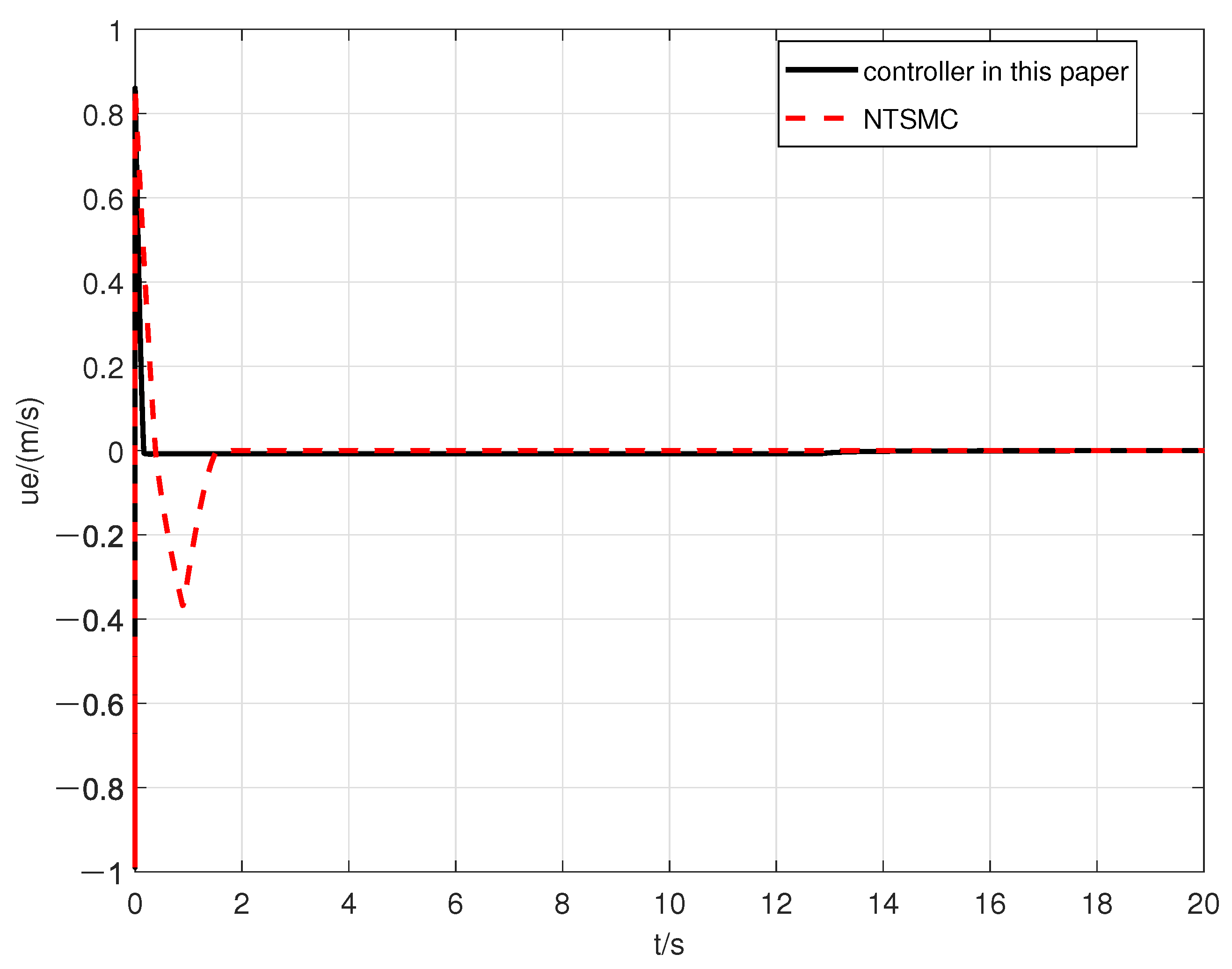
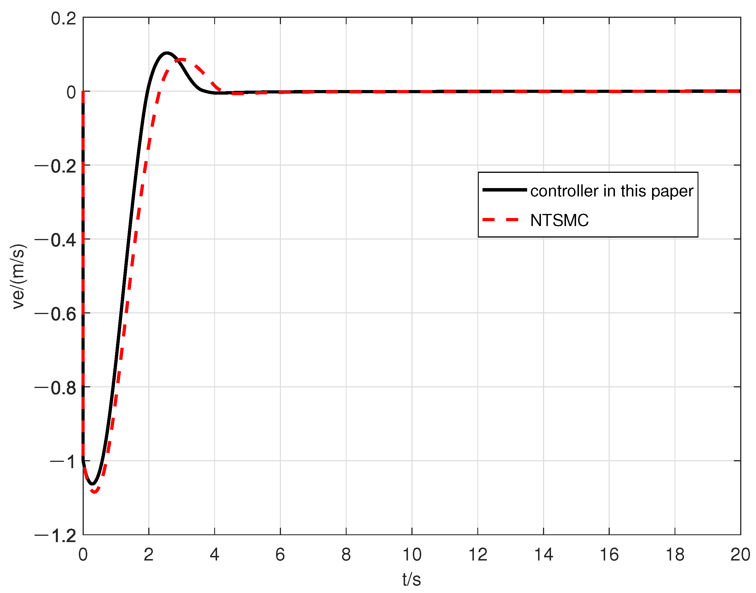
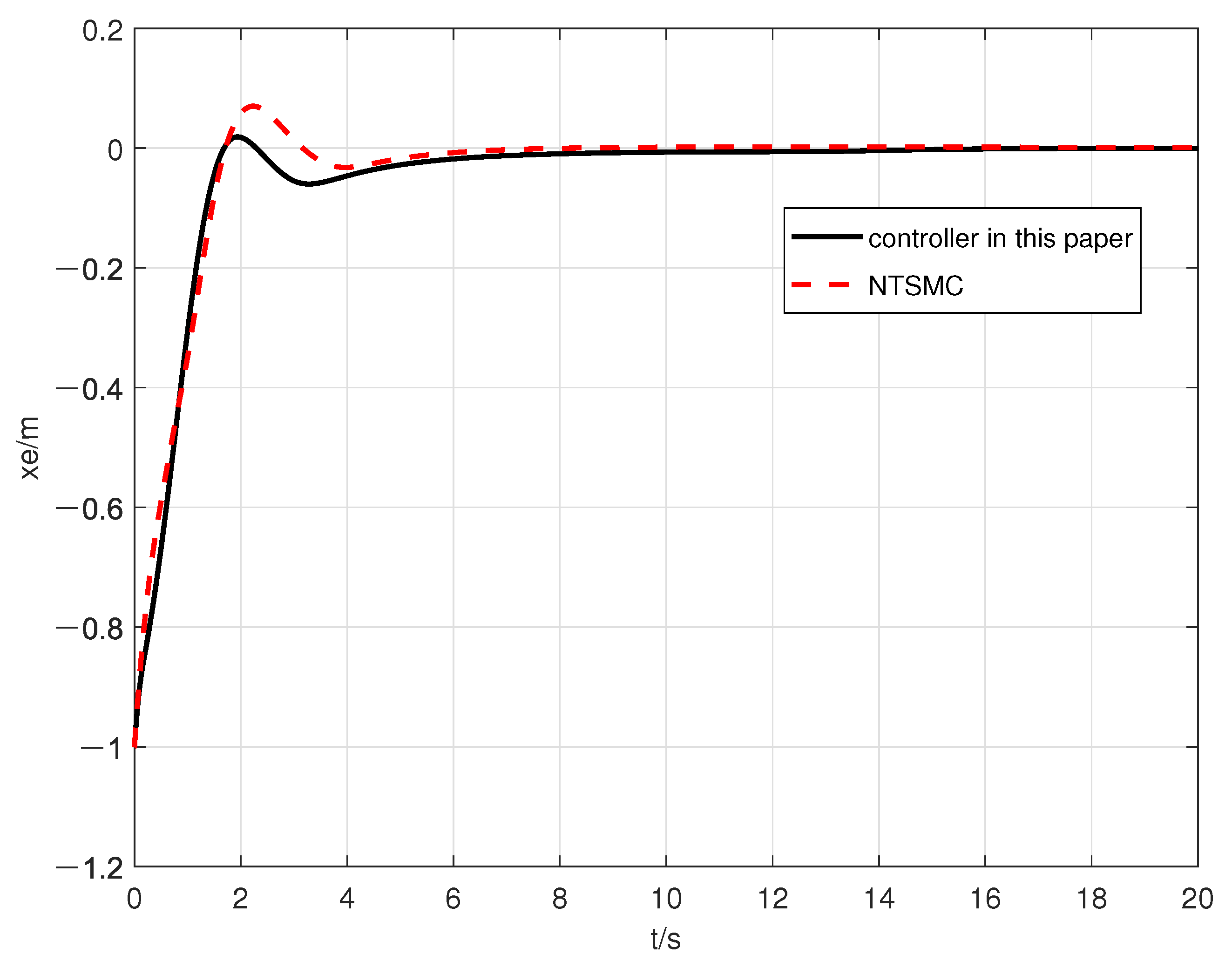
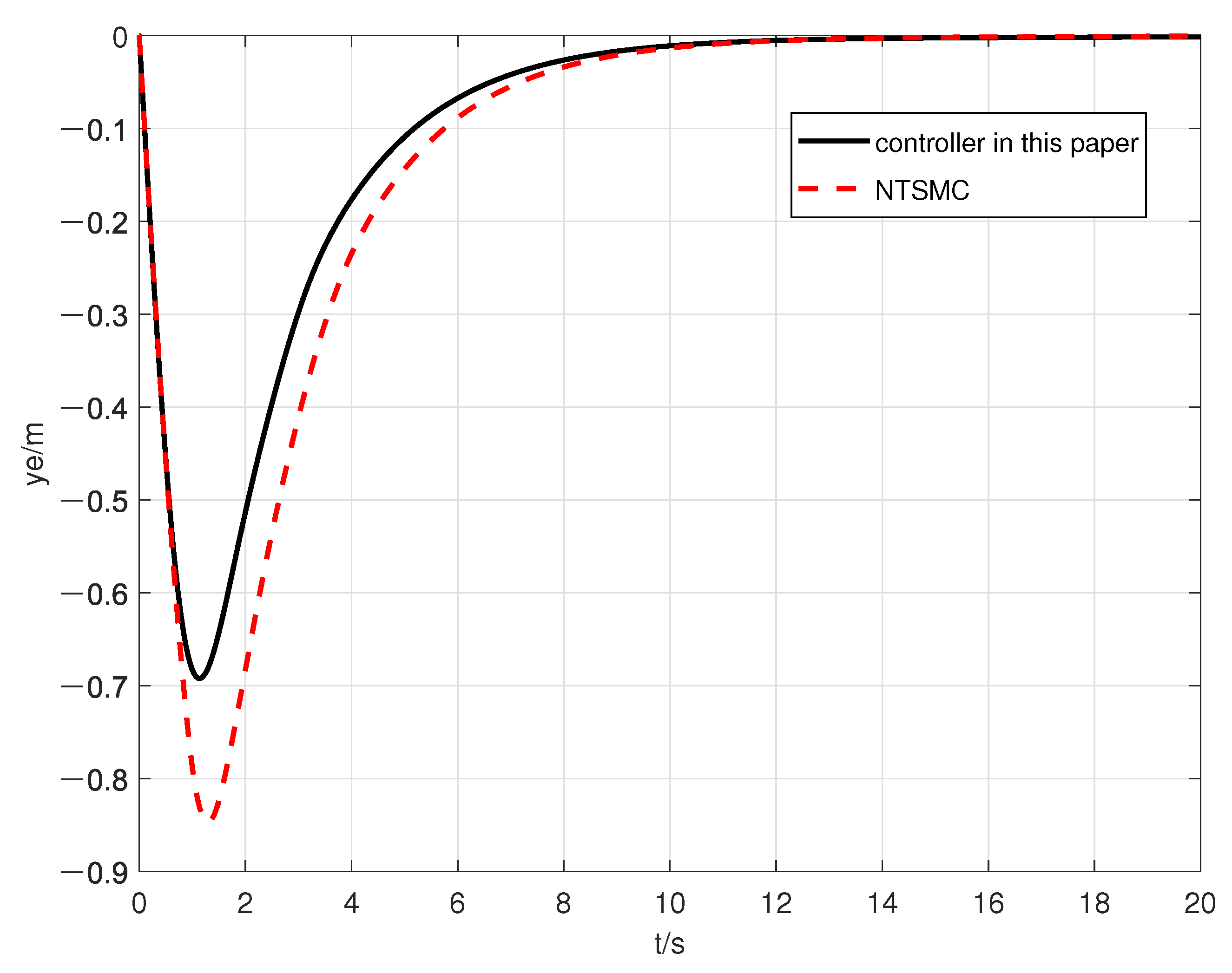
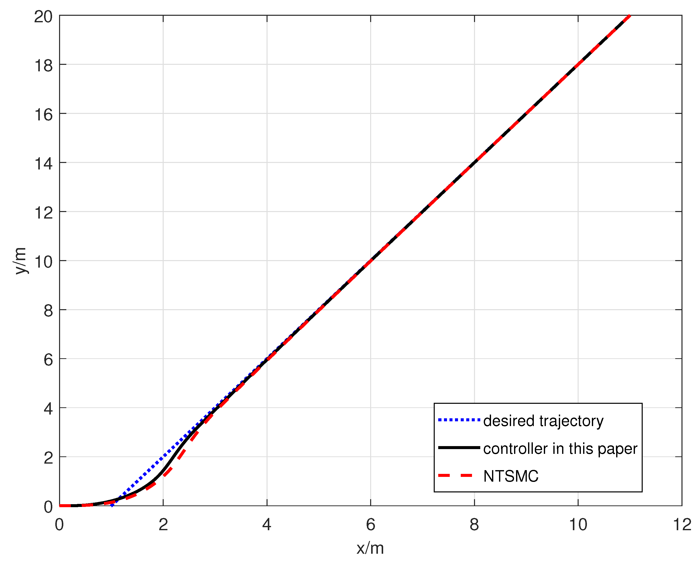
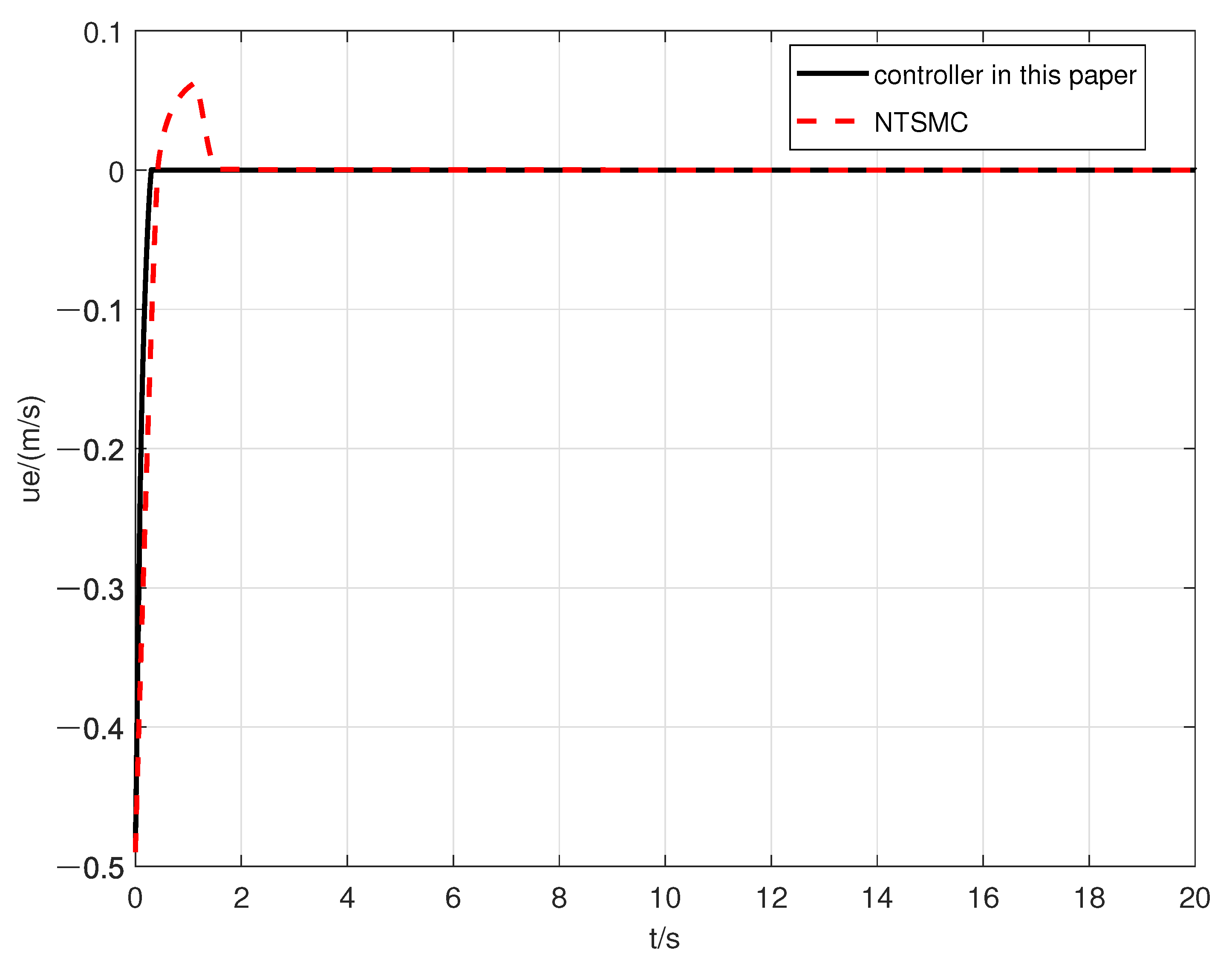
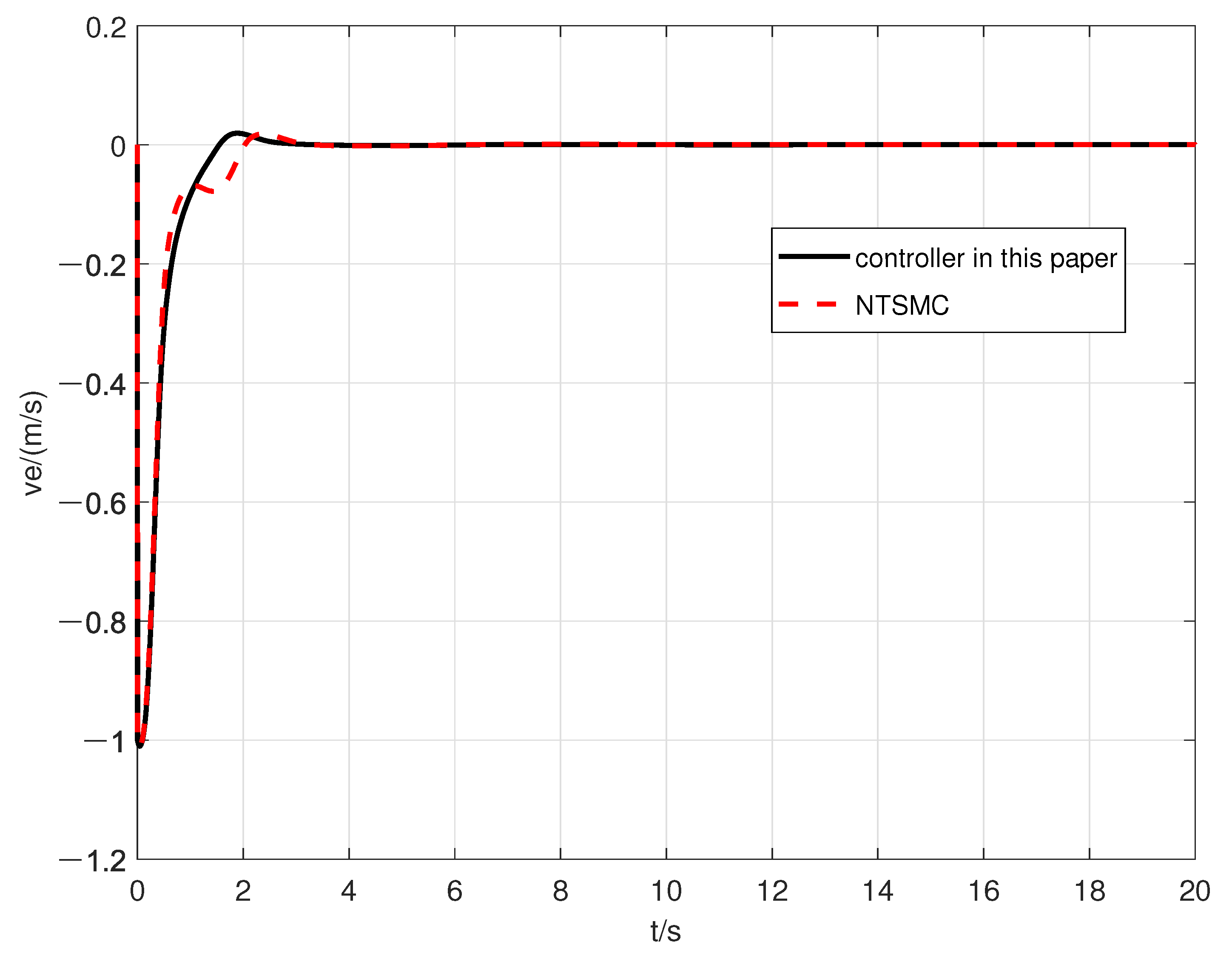
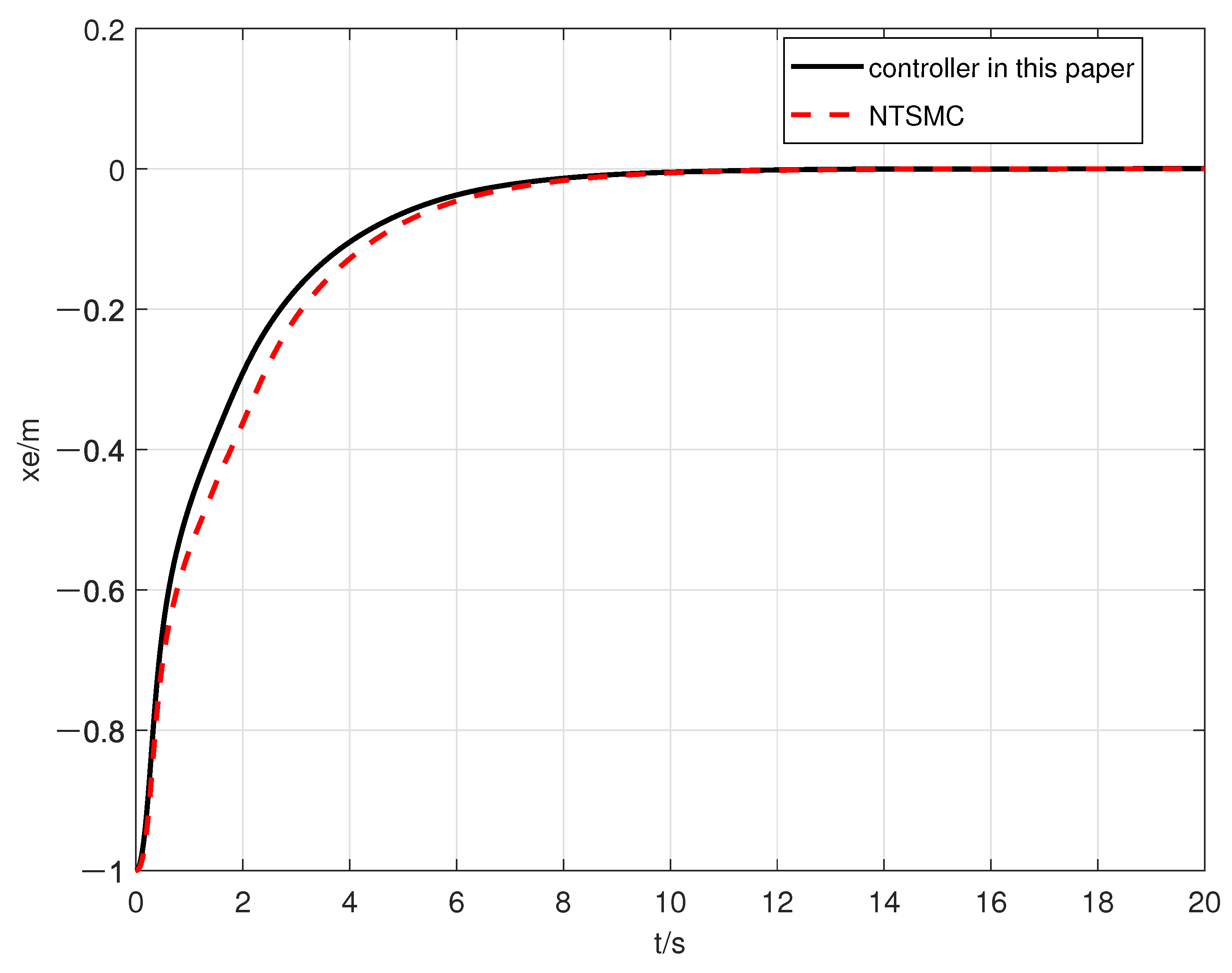
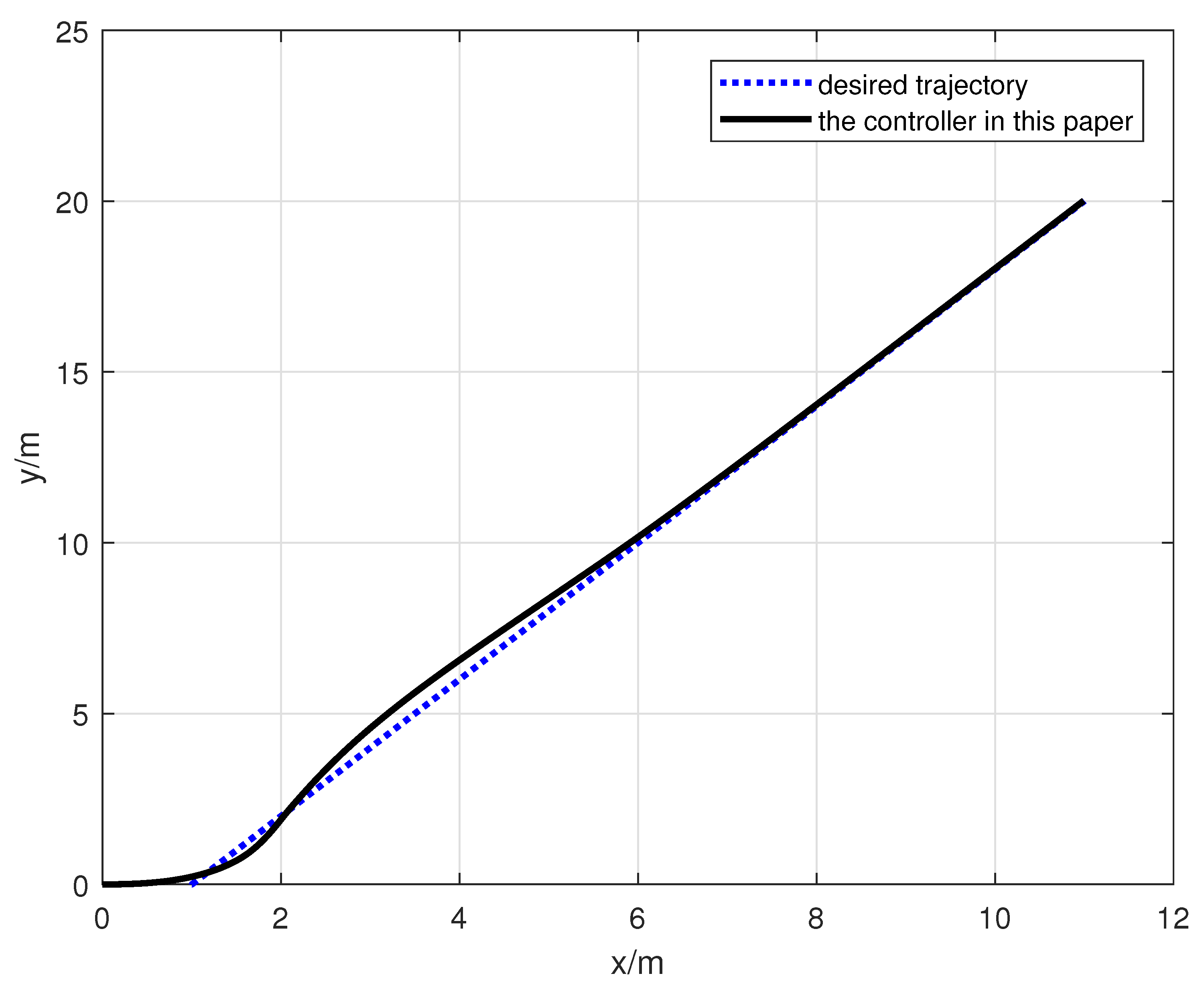
The aim is to create control inputs τ u , τ r that enable the underactuated AUV to track the expected trajectory, i.e., ( x ( t ) , y ( t ) ) ( x d ( t ) , y d ( t ) ) . Based on the analysis of the trajectory error equation, two phases make up the controller design process. Firstly, the expected forward and backward velocity u d and lateral velocity v d are designed to make trajectory tracking error converge to 0. Then, based on nonsingular fast TSM, the nonsingular fast TSM surfaces S 1 and S 2 are constructed. Furthermore, the appropriate control inputs τ u , τ r are developed to ensure that the speeds of the underactuated AUV can converge to the designed expected value.
Based on the desired forward and backward velocity and lateral velocity, the following theorem ensures that the trajectory tracking error will converge.
Theorem 2.
The expected forward and backward velocity and lateral velocity are built as follows:
u d v d = cos ψ sin ψ sin ψ cos ψ x ˙ d + g x tanh ( h x x e / g x ) y ˙ d + g y tanh ( h y y e / g y )
If speed tracking error converges to 0, trajectory tracking error can asymptotically converge to 0, where g x > 0 , h x > 0 , g y > 0 , h y > 0 .
Proof. 
From (1) and (2), we have
u = x ˙ cos ψ + y ˙ sin ψ
v = x ˙ sin ψ + y ˙ cos ψ
Substituting (16) and (17) into (11) and (12), respectively, yields
u e v e = cos ψ sin ψ sin ψ cos ψ x ˙ y ˙ u d v d
Substituting (15) into (18) yields
u e v e = R x ˙ e g x tanh ( h x x e / g x ) y ˙ e g y tanh ( h y y e / g y )
where R = cos ψ sin ψ sin ψ cos ψ .
According to (19), since R = 1 , R is nonsingular, when x ˙ e g x tanh ( h x x e / g x ) and y ˙ e g y tanh ( h y y e / g y ) converge to 0, u e and v e converge to 0.
When the speed tracking error converges to 0, we obtain
x ˙ e = g x tanh ( h x x e / g x )
y ˙ e = g y tanh ( h y y e / g y )
To guarantee that x e and y e converge to 0, the Lyapunov function is selected as
V 1 = 1 2 x e 2 + 1 2 y e 2
Taking the derivative of (22) yields
V ˙ 1 = x e x ˙ e + y e y ˙ e = g x x e tanh ( h x x e / g x ) g y y e tanh ( h y y e / g y )
From (23), V ˙ 1 < 0 is obtained when ( x e , y e ) ( 0 , 0 ) since h x > 0 , g x > 0 , g y > 0 , h y > 0 . Thus, x e and y e asymptotically converge to 0. Thus, when the forward and backward velocity and lateral velocity converge to the expected velocity values shown in (18), x e and y e asymptotically converge to 0. □
Remark 1.
The DVTER is built according to the kinematics and kinetic equation of the underactuated AUV, which avoids the limitation of deriving the expected speed value from the expected position value in [29]. Moreover, by designing the the expected speed values, position tracking errors can converge to 0.
Based on the above analysis, the main theorem is shown as follows.
Theorem 3.
For speed error tracking system (13) and (14), the following controllers are designed:
τ u = ( 1 / M 1 β 1 γ 2 ) s i g n 2 γ 2 ( u e ) { [ 1 + α 1 γ 1 s i g n γ 1 1 ( u ˜ e ) ] u e k 1 s i g n ( S 1 ) l 1 S 1 } X u u a 23 v r + u ˙ d
τ r = [ 1 / M 3 ( u d + M 2 a 13 u ) ] { ( 1 / β 2 γ 2 ) s i g n 2 γ 2 ( v ˙ e ) [ v ˙ e α 2 γ 1 v ˙ e s i g n γ 1 1 ( v e ) ] M 2 ( Y v v ˙ + a 13 u ˙ r ) + T } N r r a 12 u v
If the parameters are selected satisfying α 1 > 0 , α 2 > 0 , 1 < γ 2 < 2 , γ 1 > γ 2 , β 1 > 0 , β 2 > 0 , the speed tracking error system is stable in finite time, that is, the speed tracking errors u e , v e converge to 0 in finite time.
Proof. 
Taking the derivative of (18) yields
u ˙ d v ˙ d = v d r u d r + cos ψ sin ψ sin ψ cos ψ   x ¨ d h x x ˙ e sech 2 ( h x x e / g x ) y ¨ d h y y ˙ e sech 2 ( h y y e / g y )
Taking the derivative of v ˙ d yields
v ¨ d = T u d r ˙
where T = A sin ψ + B cos ψ x ¨ d r cos ψ y ¨ d r sin ψ u ˙ d r + χ 1 r cos ψ + χ 2 r sin ψ + χ ˙ 1 sin ψ χ ˙ 2 cos ψ , A = d x ¨ d / d t , B = d y ¨ d / d t , χ 1 = h x x ˙ e sech 2 ( h x x e / g x ) , χ 2 = h y y ˙ e sech 2 ( h y y e / g y ) .
The nonsingular fast TSM surfaces are developed as follows:
S 1 = u ˜ e + α 1 s i g n γ 1 ( u ˜ e ) + β 1 s i g n γ 2 ( u e )
S 2 = v e + α 2 s i g n γ 1 ( v e ) + β 2 s i g n γ 2 ( v ˙ e )
where u ˜ e = 0 t u e ( τ ) d τ . Both γ 1 and γ 2 have the form p / q , and p, q are both odd positive numbers.
By taking the derivative of (28) and (29) separately, we obtain
S ˙ 1 = u e + α 1 γ 1 u e s i g n γ 1 1 ( u ˜ e ) + β 1 γ 2 u ˙ e s i g n γ 2 1 ( u e ) = [ 1 + α 1 γ 1 s i g n γ 1 1 ( u ˜ e ) ] u e + β 1 γ 2 s i g n γ 2 1 ( u e ) [ M 1 ( X u u + a 23 v r + τ u ) u ˙ d ]
S ˙ 2 = v ˙ e + α 2 γ 1 v ˙ e s i g n γ 1 1 ( v e ) + β 2 γ 2 v ¨ e s i g n γ 2 ( v ˙ e ) = [ 1 + α 2 γ 1 s i g n γ 1 1 ( v e ) ] v ˙ e + β 2 γ 2 s i g n γ 2 ( v ˙ e ) [ M 2 ( Y v v ˙ + a 13 u ˙ r ) T + M 3 ( u d + M 2 a 13 u ) ( N r r + a 12 u v + τ r ) ]
Select the Lyapunov function as
V 2 = 1 2 S 1 2 + 1 2 S 2 2
Taking the derivative of (32) and substituting (30) and (31) into it, one has
V ˙ 2 = S 1 S ˙ 1 + S 2 S ˙ 2 = S 1 { [ 1 + α 1 γ 1 s i g n γ 1 1 ( u ˜ e ) ] u e + β 1 γ 2 s i g n γ 2 1 ( u e ) [ M 1 ( X u u + a 23 v r + τ u ) u ˙ d ] } + S 2 { [ 1 + α 2 γ 1 s i g n γ 1 1 ( v e ) ] v ˙ e + β 2 γ 2 s i g n γ 2 ( v ˙ e ) [ M 2 ( Y v v ˙ + a 13 u ˙ r ) T + M 3 ( u d + M 2 a 13 u ) ( N r r + a 12 u v + τ r ) ] }
Substituting (24) and (25) into (33) yields
V ˙ 2 = S 1 S ˙ 1 + S 2 S ˙ 2 = k 1 S 1 2 l 1 S 1 k 2 S 2 2 l 2 S 2
According to (34), since l 1 > 0 , l 2 > 0 , k 1 0 , k 2 0 , it can be obtained that V ˙ 2 < 0 for ( S 1 , S 2 ) 0 . Therefore, S 1 , S 2 converge to 0 in finite time.
When S 1 = S 2 = 0 , we obtain
u ˜ e + α 1 s i g n γ 1 ( u ˜ e ) + β 1 s i g n γ 2 ( u e ) = 0
v e + α 2 s i g n γ 1 ( v e ) + β 2 s i g n γ 2 ( v ˙ e ) = 0
According to Lemma 1, the states u e , v e , and v ˙ e will converge to 0 in finite time. In summary, the forward and backward velocity and lateral velocity converge to the expected values shown in (15) in a finite time. According to Theorem 1, x e and y e asymptotically converge to 0.
When v ˙ e convergs to 0, it can be obtained from (14) that
v ˙ d = M 2 ( Y v v d + a 13 u d r )
According to (26), we obtain
v ˙ d = u d r sin ψ [ x ¨ d h x x ˙ e sech 2 ( h x x e / g x ) ] + cos ψ [ y ¨ d h y y ˙ e sech 2 ( h y y e / g y ) ]
Substituting (38) into (37) yields
sin ψ [ x ¨ d h x x ˙ e sech 2 ( h x x e / g x ) ] + cos ψ [ y ¨ d h y y ˙ e sech 2 ( h y y e / g y ) ] = ( M 2 a 13 + 1 ) u d r + M 2 Y v v d
Since u d > 0 , it is concluded from (15), (20), and (21) that u d , v d , x ˙ e , and y ˙ e are both bounded. Thus, the yaw rate r is bounded.
Select the following Lyapunov function:
V 3 = 1 2 r 2
Taking the derivative of (41) and substituting (6) into it, one has
V ˙ 3 = r r ˙ = M 3 r ( N r r + a 12 u v + τ r )
Because of N r < 0 , M 3 > 0 , in order to make V ˙ 3 < 0 , it needs to satisfy
N r r > a 12 u v + τ r
Since V ˙ 3 < 0 , V 3 is decreasing, r is decreasing. In summary, the designed controller can ensure that the yaw rate r is bounded. When the condition (42) is satisfied, the yaw rate r can asymptotically converge to 0. □
Remark 2.
Since 1 < γ 2 < 2 , γ 1 > γ 2 , it can be noted that the controllers (26) and (27) do not contain any singularity. Regarding the nonsingular fast TSM surface, such as S 1 , when the system state remains away from equilibrium, α 1 s i g n γ 1 ( u ˜ e ) dominates the convergence rate and ensures a fast convergence rate. When the system state approaches equilibrium, the dominant term β 1 s i g n γ 2 ( u e ) determines finite-time convergence. Moreover, it is proved that compared to NTSM, NFTSM’s convergence time is shorter in [27].
Remark 3.
To further weaken chattering, a saturation function can be employed instead of a symbol function in the constructed controller, where
s a t ( S ) = 1 , S < φ S / φ , φ < S < φ 1 , S > φ
and by adjusting the thickness of boundary layer φ, the system state can converge to a sliding mode surface.
Remark 4.
Compared with the fast TSM controller (FTSMC) [30], the designed controller (26) and (27) can retain the advantages of FTSMC while ensuring nonsingularity. Different from NTSMC [21], the designed controller (26) and (27) has better performance, especially when the initial state is far away from the equilibrium. Thus, the designed control strategy enables the underactuated AUV to have faster tracking speed.
Remark 5.
In [22], the nonsingular fast terminal sliding mode approach is also studied for the trajectory tracking control of the AUV. However, this paper has a few differences from [22]. (1) In [22], the convergence of position tracking error cannot be guaranteed by the convergence of velocity tracking error. In this paper, the DVTER is built according to the kinematics equation and kinetic equation of the underactuated AUV. And the convergence of the position tracking errors x e , y e can be guaranteed by stabilizing velocity tracking errors u e and v e . (2) In [22], a sliding mode surface is designed based on the position trajectory tracking error. However, in order to achieve more precise control, the variables on the horizontal and vertical axes are not combined into one variable in this paper. Two sliding mode surfaces are designed based on forward and backward velocity tracking error u e , and lateral velocity tracking error v e , respectively. Thus, when constructing the controller based on the designed sliding surfaces, more adjustable parameters can be introduced in the controller, which is more general and flexible.
Remark 6.
In [15], the trajectory tracking controller is designed for an underactuated AUV based on contraction theory. In [31], a trajectory tracking control scheme is designed for underactuated underwater vehicles on the basis of velocity transformation. In [32], based on extended state observer and backstepping, a trajectory tracking control method is developed for an AUV under quantized state feedback and ocean disturbances. However, the convergence speed is not considered in these methods. Moreover, the convergence of position tracking error also cannot be guaranteed by the convergence of velocity tracking error. Different from [15,31,32], the convergence speed is improved in this paper, and the convergence of position tracking error can be guaranteed by the convergence of velocity tracking error under the developed controller.

4. Simulation

The model parameters of the considered underactuated AUV are [14]: X u = 8.8065 kg / s ,   Y v = 65.5457 kg / s ,   N r ˙ = 35.5 kg · m 2 ,   m = 30.48 kg ,   N r = 6.7352 kg / s ,   X u ˙ = 0.93 kg ,   I z = 3.45 kg · m 2 ,   Y v ˙ = 35.5 kg . Next, the two situations below are provided to illustrate the validity of the designed control technique.
In theory, selecting a larger value for γ 1 can lead to faster convergence when the system state stays far from equilibrium. The parameters γ 1 , γ 2 are often selected as 1 < γ 2 < 2 , γ 1 > γ 2 . Both γ 1 and γ 2 have the form p / q , and both p and q are positive odd numbers. When choosing the parameters, the values of l 1 , l 2 , g x , h x , g y , and h y > 0 are first set within a suitable range. Next, adjust γ 1 and γ 2 , and then tune α 1 , α 2 , β 1 , and β 2 . Trial and error can be employed to achieve satisfactory control performance.
Case 1: The desired linear trajectory is
x d = 0.5 t + 1 y d = 0.25 t + 0.5
The parameters are selected as g x = g y = 2 ,   h x = h y = 0.5 ,   u ˜ e ( 0 ) = 0.05 ,   v ˜ e ( 0 ) = 0 , φ = 0.01 ,   α 1 = α 2 = 1 ,   β 1 = β 2 = 1.3 ,   γ 1 = 7 / 3 ,   γ 2 = 5 / 3 . For the sake of comparison, the NTSMC [21] is considered. The simulation results are shown in Figure 2, Figure 3, Figure 4, Figure 5 and Figure 6.
Figure 2 shows the curves of forward and backward speed error u e with the designed controller and NTSMC, respectively. With both controllers, u e can converge to 0 within a finite time. Under the action of the designed controller, the expected forward and backward speed is tracked at 0.25 s. Under the action of NTSMC, u e converges to 0 within 1.6s.
The curves of lateral velocity tracking error v e are shown in Figure 3. The designed controller enables v e to converge to 0 within 3.6s. NTSMC makes v e converge to 0 within 4.5 s. Under the action of these two controllers, v e can converge to 0 in a finite time, but the designed controller makes the convergence speed of v e faster.
To present the comparison results more intuitively, the convergence time of u e and v e is shown in Table 1 by comparing with the method in [21]. The convergence time of u e and v e is reduced by 83.3% and 20% compared with [21], respectively.
The curves of x e , y e are displayed as Figure 4 and Figure 5, respectively. From Figure 4 and Figure 5, x e , y e can converge to 0 in a finite time, and the designed controller can make position tracking error have a faster convergence speed.
Figure 6 gives the actual motion trajectory of the underactuated AUV. It can be seen that the underactuated AUV can track expected straight-line trajectory with two controllers, and the tracking effect is better under the action of the designed controller in this paper. Compared with NTSMC, the designed controller enables the underactuated AUVs to have faster tracking speed.
Case 2: To verify the tracking effect of the designed controller on different trajectories, curve trajectories were further selected to verify the effectiveness of the controller. The desired trajectory is:
x d = cos t y d = sin t
The parameters are chosen as g x = g y = 2 , h x = h y = 0.5 , u ˜ e ( 0 ) = 0.05 , v ˜ e ( 0 ) = 0 , φ = 0.01 , α 1 = 1 , α 2 = 1.5 , β 1 = 1.5 , β 2 = 2 , γ 1 = 7 / 3 , γ 2 = 5 / 3 . Similarly, the simulation results are compared with the NTSMC, as shown in Figure 7, Figure 8, Figure 9, Figure 10 and Figure 11.
Figure 7 shows the curves of forward and backward velocity error u e . From Figure 7, u e can converge to 0 with the two controllers in a finite time. Under the action of the designed controller, the desired forward and backward speed is tracked at 0.4 s. Under the action of NTSMC, u e converges to 0 within 1.58 s. Thus, the tracking effect with the designed controller is better.
The curves of lateral velocity tracking error v e are shown in Figure 8. The designed controller enables v e to converge to 0 within 2.5 s. NTSMC makes the v e converge to 0 within 3.3 s. Under the action of these two controllers, v e can converge to 0 in a finite time, and the designed controller makes the convergence speed of lateral velocity error faster.
To present the comparison results more intuitively, the convergence time of velocity tracking errors u e and v e is shown in Table 2 by comparing with the method in [21]. The convergence time of u e and v e is reduced by 74.7% and 24.2% compared with [21], respectively.
The curves of x e , y e are given in Figure 9 and Figure 10. With both controllers, the position tracking errors converge to 0 in a finite time, and the designed controller makes the convergence speed of position tracking error faster.
Figure 11 shows the actual motion trajectory of the underactuated AUV with two controllers. It is shown that both controllers can achieve trajectory tracking, and the tracking performance with the designed controller is better. By comparison, the tracking performance with the designed controller is better than NTSMC, making the underactuated AUV have faster tracking speed.
As a result, it is obtained obviously from the simulation results that the constructed technique can achieve better tracking performance than the control method in [21].
To show the robustness of the constructed technique, the kinematic and dynamic equations including disturbances [21] are studied.
x ˙ = u cos ψ v sin ψ y ˙ = u sin ψ + v cos ψ ψ ˙ = r u ˙ = M 1 ( X u u + a 23 v r + τ u ) + d 1 ( t ) v ˙ = M 2 ( Y v v + a 13 u r ) r ˙ = M 3 ( N r r + a 12 u v + τ r ) + d 2 ( t )
where d 1 ( t ) = 0.7 , d 2 ( t ) = 0.45 . For the following desired trajectory,
x d = 0.5 t + 1 y d = 0.25 t + 0.5 ,
the simulation results are displayed in Figure 12, Figure 13, Figure 14, Figure 15 and Figure 16.
It is obtained from Figure 11, Figure 12, Figure 13, Figure 14, Figure 15 and Figure 16 that trajectory tracking is achieved with the designed controller despite disturbances acting on the AUV. Thus, it can be concluded that the developed control method is robust under disturbances.

5. Conclusions

Aiming at the trajectory tracking control issue of an underactuated AUV in the horizontal plane, a trajectory tracking controller is constructed on the basis of nonsingular fast TSM. The DVTER is constructed according to the kinematics and kinetic equation. By designing the expected speed value, the limitation of deriving the expected speed value from the expected position value is avoided. The designed controller retains the advantages of FTSMC while ensuring nonsingularity. Compared with NTSMC, the designed controller enables the underactuated AUV to have faster tracking speed. Finally, simulation results show the effectiveness of the developed technique.

Author Contributions

Methodology, writing—original draft preparation, Y.W.; writing—review and editing, Z.D. All authors have read and agreed to the published version of the manuscript.

Funding

This work is supported by the Natural Science Foundation of Shandong Province (ZR2021MF133, ZR2023QF026) and Young Doctor Research Foundation of Yantai University (JS22B175).

Institutional Review Board Statement

Not applicable.

Informed Consent Statement

Not applicable.

Data Availability Statement

The original contributions presented in the study are included in the article, further inquiries can be directed to the corresponding author.

Conflicts of Interest

The authors have no conflicts of interest to declare.

References

  1. Yao, J.; Yang, J.; Zhang, C.; Zhang, J.; Zhang, T. Autonomous Underwater Vehicle Trajectory Prediction with the Nonlinear Kepler Optimization Algorithm–Bidirectional Long Short-Term Memory–Time-Variable Attention Model. J. Mar. Sci. Eng. 2024, 12, 1115. [Google Scholar] [CrossRef]
  2. Shao, G.; Wan, L.; Xu, H. Formation Control of Autonomous Underwater Vehicles Using an Improved Nonlinear Backstepping Method. J. Mar. Sci. Eng. 2024, 12, 878. [Google Scholar] [CrossRef]
  3. Gutnik, Y.; Groper, M. Terminal Phase Navigation for AUV Docking: An Innovative Electromagnetic Approach. J. Mar. Sci. Eng. 2024, 12, 192. [Google Scholar] [CrossRef]
  4. Hedayati Khodayari, M.; Pariz, N.; Balochian, S. Admissibility analysis for autonomous underwater vehicle based on descriptor model with time-varying delay. J. Vib. Control 2022, 28, 3302–3314. [Google Scholar] [CrossRef]
  5. Huang, H.; Wen, X.; Niu, M.; Miah, M.S.; Wang, H.; Gao, T. Multi-Objective Path Planning of Autonomous Underwater Vehicles Driven by Manta Ray Foraging. J. Mar. Sci. Eng. 2024, 12, 88. [Google Scholar] [CrossRef]
  6. Zhang, B.; Ji, D.; Liu, S.; Zhu, X.; Xu, W. Autonomous Underwater Vehicle navigation: A review. Ocean Eng. 2023, 273, 113861. [Google Scholar] [CrossRef]
  7. Sahoo, A.; Dwivedy, S.K.; Robi, P.S. Advancements in the field of autonomous underwater vehicle. Ocean Eng. 2019, 181, 145–160. [Google Scholar] [CrossRef]
  8. Jiang, X.S.; Feng, X.S.; Wang, D.T. Unmanned Underwater Vehicles; Liaoning Science and Technology Press: Shenyang, China, 2000. [Google Scholar]
  9. Cho, G.R.; Li, J.H.; Park, D.; Jung, J.H. Robust trajectory tracking of autonomous underwater vehicles using back-stepping control and time delay estimation. Ocean Eng. 2020, 201, 107131. [Google Scholar] [CrossRef]
  10. Xu, J.; Wang, M.; Qiao, L. Backstepping-based controller for three-dimensional trajectory tracking of underactuated unmanned underwater vehicles. Control Theory Appl. 2014, 31, 1589–1596. [Google Scholar]
  11. Yan, Z.; Wang, M.; Xu, J. Global adaptive neural network control of underactuated autonomous underwater vehicles with parametric modeling uncertainty. Asian J. Control 2019, 21, 1342–1354. [Google Scholar] [CrossRef]
  12. Xia, G.Q.; Yang, Y. FNN-based L2 following control of underactuated autonomous underwater vehicles. Control Decis. 2013, 28, 351–356. [Google Scholar]
  13. Ma, L.M. Global chattering-free sliding mode trajectory tracking control of underactuated autonomous underwater vehicles. CAAI Trans. Intell. Syst. 2016, 11, 200–207. [Google Scholar]
  14. Elmokadem, T.; Zribi, M.; Youcef-Toumi, K. Trajectory tracking sliding mode control of underactuated AUVs. Nonlinear Dyn. 2016, 84, 1079–1091. [Google Scholar] [CrossRef]
  15. Ma, C.; Jia, J.; Zhang, T.; Wu, S.; Jiang, D. Horizontal trajectory tracking control for underactuated autonomous underwater vehicles based on contraction theory. J. Mar. Sci. Eng. 2023, 11, 805. [Google Scholar] [CrossRef]
  16. Feng, Y.; Yu, X.; Man, Z. Non-singular terminal sliding mode control of rigid manipulators. Automatica 2002, 38, 2159–2167. [Google Scholar] [CrossRef]
  17. Wang, Z.; Li, S.; Fei, S. Nonsingular terminal sliding mode guidance law. J. Southeast Univ. 2009, 39, 87–90. [Google Scholar]
  18. Feng, Y.; Yu, X.; Han, F. On nonsingular terminal sliding-mode control of nonlinear systems. Automatica 2013, 49, 1715–1722. [Google Scholar] [CrossRef]
  19. Fei, J.; Chen, Y.; Liu, L.; Fang, Y. Fuzzy multiple hidden layer recurrent neural control of nonlinear system using terminal sliding-mode controller. IEEE Trans. Cybern. 2021, 52, 9519–9534. [Google Scholar] [CrossRef] [PubMed]
  20. Nekoukar, V.; Dehkordi, N.M. Robust path tracking of a quadrotor using adaptive fuzzy terminal sliding mode control. Control Eng. Pract. 2021, 110, 104763. [Google Scholar] [CrossRef]
  21. Elmokadem, T.; Zribi, M.; Youcef-Toumi, K. Terminal sliding mode control for the trajectory tracking of underactuated Autonomous Underwater Vehicles. Ocean Eng. 2017, 129, 613–625. [Google Scholar] [CrossRef]
  22. Yang, X.; Yan, J.; Hua, C.; Guan, X. Trajectory tracking control of autonomous underwater vehicle with unknown parameters and external disturbances. IEEE Trans. Syst. Man Cybern. Syst. 2021, 51, 1054–1063. [Google Scholar] [CrossRef]
  23. Fossen, T.I. Marine Control Systems: Guidance, Navigation, and Control of Ships, Rigs and Underwater Vehicles; Marine Cybernetics: Trondheim, Norway, 2002. [Google Scholar]
  24. Park, B.S. Adaptive formation control of underactuated autonomous underwater vehicles. Ocean Eng. 2015, 96, 1–7. [Google Scholar] [CrossRef]
  25. Tang, S.C. Modeling and Simulation of the Autonomous Underwater Vehicle, Autolycus. Ph.D. Dissertation, Massachusetts Institute of Technology, Cambridge, MA, USA, 1999. [Google Scholar]
  26. Alberti, J. Modeling and Model Identification of Autonomous Underwater Vehicles. Ph.D. Dissertation, Naval Postgraduate School, Monterey, CA, USA, 2015. [Google Scholar]
  27. Yang, L.; Yang, J. Nonsingular fast terminal sliding-mode control for nonlinear dynamical systems. Int. J. Robust Nonlinear Control 2011, 21, 1865–1879. [Google Scholar] [CrossRef]
  28. Brockett, R.W. Asymptotic stability and feedback stabilization. Differ. Geom. Control. Theory 1983, 27, 181–191. [Google Scholar]
  29. Ashrafiuon, H.; Muske, K.R.; McNinch, L.C.; Soltan, R.A. Sliding-mode tracking control of surface vessels. IEEE Trans. Ind. Electron. 2008, 55, 4004–4012. [Google Scholar] [CrossRef]
  30. Zhong, Y.; Yang, Y.; He, K.; Chen, C. Fast terminal sliding-mode control based on unknown input observer for the tracking control of underwater vehicles. Ocean Eng. 2022, 264, 112480. [Google Scholar] [CrossRef]
  31. Herman, P. Trajectory Tracking Nonlinear Controller for Underactuated Underwater Vehicles Based on Velocity Transformation. J. Mar. Sci. Eng. 2023, 11, 509. [Google Scholar] [CrossRef]
  32. Zhou, B.; Su, Y.; Huang, B.; Wang, W.; Zhang, E. Trajectory tracking control for autonomous underwater vehicles under quantized state feedback and ocean disturbances. Ocean Eng. 2022, 256, 111500. [Google Scholar] [CrossRef]
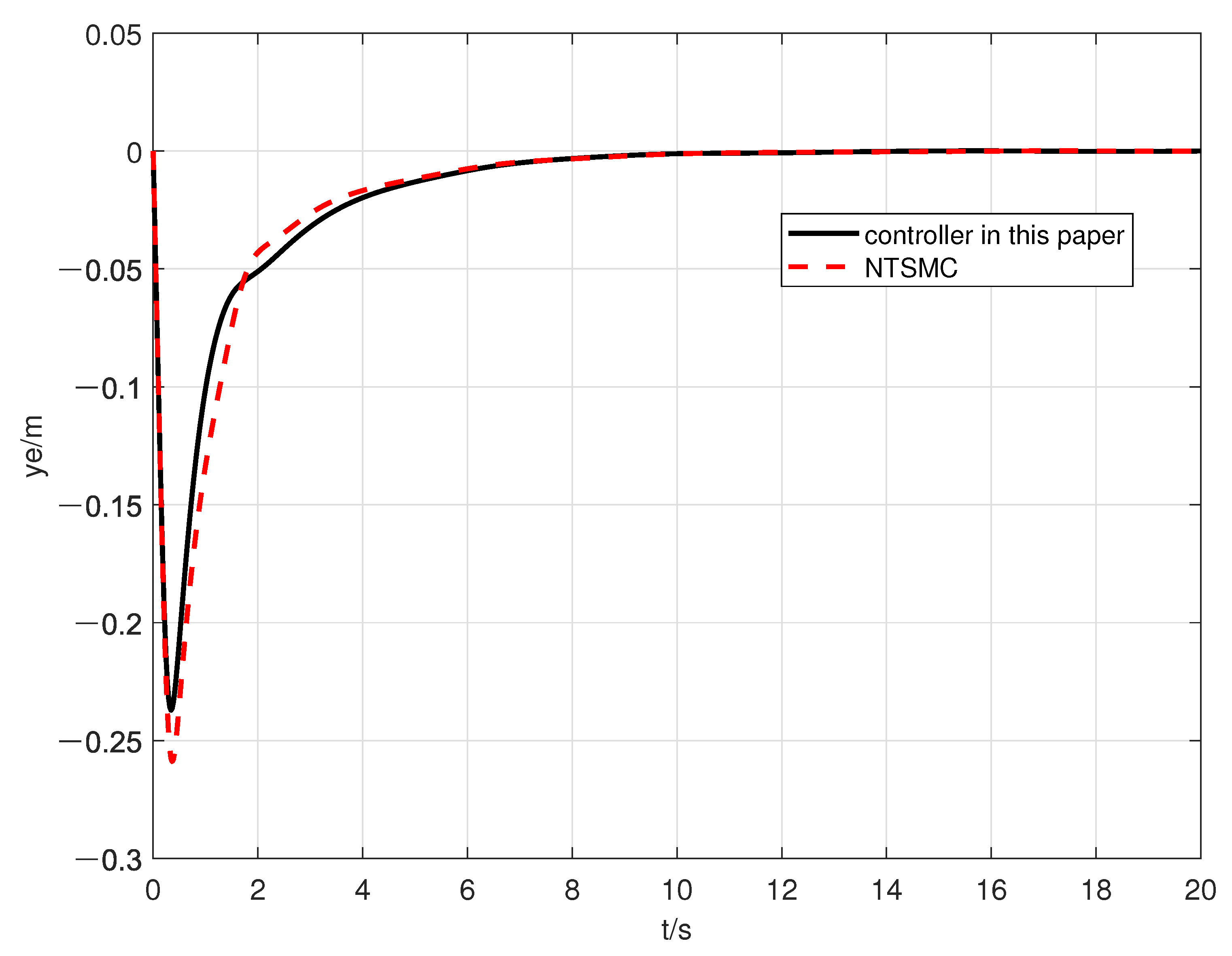
Figure 1. Inertial coordinate and body coordinate.
Jmse 12 01442 g001
Figure 2. The forward and backward velocity error u e .
Jmse 12 01442 g002
Figure 3. The lateral velocity error v e .
Jmse 12 01442 g003
Figure 4. The position tracking error x e .
Jmse 12 01442 g004
Figure 5. The position tracking error y e .
Jmse 12 01442 g005
Figure 6. The actual trajectory in Case 1.
Jmse 12 01442 g006
Figure 7. The forward and backward velocity error u e .
Jmse 12 01442 g007
Figure 8. The lateral velocity error v e .
Jmse 12 01442 g008
Figure 9. The position tracking error x e .
Jmse 12 01442 g009
Figure 10. The position tracking error y e .
Jmse 12 01442 g010
Figure 11. The actual trajectory in Case 2.
Jmse 12 01442 g011
Figure 12. The forward and backward velocity error u e .
Jmse 12 01442 g012
Figure 13. The lateral velocity error v e .
Jmse 12 01442 g013
Figure 14. The position tracking error x e .
Jmse 12 01442 g014
Figure 15. The position tracking error y e .
Jmse 12 01442 g015
Figure 16. The actual trajectory of underactuated AUV with the disturbances.
Jmse 12 01442 g016
Table 1. The convergence time of velocity tracking errors.
ErrorThe Designed Controller in This PaperThe Controller in [21]
u e 0.25 s1.5 s
v e 3.6 s4.5 s
Table 2. The convergence time of velocity tracking errors.
ErrorThe Designed Controller in This PaperThe Controller in [21]
u e 0.4 s1.58 s
v e 2.5 s3.3 s
Disclaimer/Publisher’s Note: The statements, opinions and data contained in all publications are solely those of the individual author(s) and contributor(s) and not of MDPI and/or the editor(s). MDPI and/or the editor(s) disclaim responsibility for any injury to people or property resulting from any ideas, methods, instructions or products referred to in the content.

