Abstract
Apart from the mechanisms of ice structure interactions under various scenarios of sea ice conditions and structural configurations, the selection of probabilistic models is crucial in order to cope with the loading uncertainty. Sea ice is the primary contributor to design loads in cold regions. In many cases, ice loads present the highest magnitude. In recent years, the probabilistic study of ice thickness, ice strength coefficient, flexural strength, ice drift speed, etc., has significantly increased, corresponding to the increasing activity of offshore operations in cold regions as well as the development of instrument technology for sea ice observation. This paper reviews existing probabilistic modes of sea ice, which are used to estimate the uncertainty of ice loading with various types of offshore structures, including vertical structures, sloping structures, and stations with floating vessels. The ISO 19906 standard is employed for the probabilistic assessment of vertical and sloping structures. The interactions between ice and structures on sloping structures are considered in both the upward and downward directions. The ice resistance method is applied for station-keeping floating vessels in ice. The key parameters of sea ice properties to estimate the design loads are studied. The effect of correlation between the key parameters of ice loads is investigated. This review shows that most existing probabilistic models are proposed for the estimation of ice loading on the various types of offshore structures.
1. Introduction
The development of offshore structures capable of enduring ice loading in the Arctic and Subarctic necessitates access to both physical and mechanical data regarding sea ice, which can be independently gathered. Concerning the physical attributes of sea ice, the predominant factor affecting ice loading for structures, whether vertical or sloping, is ice thickness. Various techniques, including satellites, submarines, upward-looking sonars (ULS), and helicopter-borne electromagnetic instruments (HEMs), among others, can measure this dimension of ice thickness. Each method offers differing levels of accuracy based on its unique attributes. For example, satellite measurements cover broad areas but lack precision, whereas HEMs provide ice thickness details solely along the helicopter’s flight path, with accuracy dependent on instrument noise and flying altitude [1]. Furthermore, the combination of average daily air temperatures from local measurement stations with ice growth models enables the estimation of nearby level ice thickness [2]. Conversely, the mechanical properties of sea ice, such as flexural strength, uniaxial strength, and ice strength coefficient, can only be obtained through experiments or field and laboratory measurements.
Zvyagin [3] implemented an analytical framework for vertical structures with the aim of probabilistically modeling ice pressure in accordance with the ISO standard formulation [4]. This methodology treats sea ice thickness and strength coefficient as random variables, employing a lognormal distribution to address the inherent uncertainty in the calculated ice pressure. Similarly, for sloping structures, a corresponding analysis may be conducted, focusing on the identification of influential parameters governing the computational outcomes. Ranta et al. [5] conducted an exhaustive examination of the failure mechanisms of level ice against inclined structures through discrete finite element analyses. Their study, encompassing both deterministic and probabilistic methodologies, elucidated the pronounced influence of ice thickness on resultant ice loading. Within deterministic analyses, the initial condition of incoming ice velocity in simulation models emerged as a significant determinant of ice load estimation. Conversely, in probabilistic analyses, it was observed that the sample size of simulated ice data significantly impacted estimated ice loads. This underscores the pivotal role of sample size in determining key statistical parameters such as mean ice load, standard deviation, and maximum load, as derived from time domain simulations [6].
Ida et al. [7] conducted a study investigating the connections between loads on various segments and the correlation between global and local loads. They discovered that the highest local line loads were caused by narrow local peak load events, with both the intensity and occurrence of these events increasing as ice strength grew. Notably, these narrow events produced local line loads that were up to four times greater than the global line load, defined as the total load on the structure divided by its width.
The management of ship and floating offshore structure positioning in cold regions presents formidable challenges. Predicting the stresses imposed on mooring systems by sea ice is particularly difficult due to the complex interplay of sea ice properties and failure mechanisms. These intricate factors introduce significant uncertainty into calculating global ice loads. A comprehensive understanding of ice dynamics, ice–structure interactions, and ship responses to ice loads is crucial for enhancing the planning and execution of ship operations. Such advancements can significantly improve the safety, structural integrity, cost-effectiveness, and operational regularity of maritime activities in icy environments. Precise vessel positioning is critical for a wide range of offshore tasks, including lifting, installation, crew transfers, emergency evacuations, drilling, tanker loading, and subsea equipment maintenance [8,9].
The drift of sea ice carries the potential to engender ice loads surpassing the operational threshold of station-keeping systems, thereby precipitating potential failures across critical components including the mooring system, dynamic positioning (DP) apparatus, ship structures, and operational equipment. To counteract these hazards, ice management strategies, such as the strategic deployment of icebreakers upstream to facilitate the creation of a continuous corridor of fragmented ice floes, are deployed. This tactical intervention seeks to curtail ice loads exerted on stationary vessels to levels deemed tolerable [9]. Nevertheless, it is imperative to acknowledge the paucity of comprehensive data stemming from diverse full-scale testing scenarios pertaining to ice management systems, with limited accessibility to such information within the public domain [10,11].
Regarding the design of the mooring system, it is imperative to consider both the potential overloading stemming from extreme environmental circumstances and the gradual accrual of fatigue-induced damage [10]. For transient operational phases, analysis focuses solely on extreme response scenarios. Conventionally, mooring system design adopts a limit state methodology, wherein the probability of overloading can be gauged by extrapolating extreme values corresponding to a designated return period, indicative of the anticipated operational duration [12]. Moreover, adherence to ISO 19906 standards (Petroleum and natural gas industries—Arctic offshore structures) permits a design approach grounded in comprehensive field experiments to accurately quantify the impact of ice actions [4]. Pertinently, in the context of enduring operations, the quantification of fatigue accumulation in mooring lines becomes requisite, particularly if the system remains static in a singular location for a duration exceeding five years [10]. The fatigue capacity of the mooring system is intricately linked to the resilience of its constituent elements such as chains, wire ropes, fiber ropes, and connecting links, often delineated through TN curves (Tension–Number curves) or SN curves (Stress–Number curves) for comprehensive assessment [10,12].
The most effective approach for creating a uniform reduction in floe sizes within drifting ice using the ice management system involves operating the icebreaker in various systematic patterns, such as circular, orbital, elliptical, linear, racetrack, etc. The icebreaker moves in the updrift direction to safeguard the stationary vessel. The primary factors influencing the choice of pattern include the speed of ice drift, thickness of the ice, rate of turning of incoming ice, and the maneuverability of the icebreaker. Employing two or more icebreakers with the same pattern can enhance the efficiency of reducing floe sizes [9].
This work reviews the uncertainty and probabilistic models involved in the interaction between ice and structures across various configurations and scenarios involving stationary vessels in ice. For fixed offshore structures, the key parameters for estimating ice loads are examined, employing random variables to describe sea ice properties. For stationary vessels in ice, the formulations used to describe ice loads during stationary periods are analyzed. Various ice management scenarios are implemented, and the different models for extreme loading on mooring lines are explored.
This work provides a comprehensive study and review of the uncertainty and probabilistic models associated with the interaction between ice and structures, focusing on a range of configurations and scenarios involving stationary vessels in ice. The study delves into the key parameters critical for estimating ice loads on fixed offshore structures, employing random variables to characterize sea ice properties such as thickness, strength coefficient, flexural strength, etc. It investigates various probabilistic models to capture the uncertainty associated with these parameters on ice load predictions. Additionally, this study explores methodologies for estimating extreme ice loads on stationary vessels, analyzing formulations used during periods when vessels are immobilized in ice. The discussion encompasses various ice management strategies implemented to mitigate ice-induced risks, including proactive measures to manage ice accumulation and control ice interactions. This study investigates different models for assessing extreme loading conditions on mooring lines, considering factors such as level ice, ice ridges, ice drift speed, and others. By comparing and contrasting these models, the study highlights advancements in predictive capabilities and identifies areas for future research and improvement in understanding stationary vessels in ice.
2. Ice Loading on Fixed and Floating Offshore Structures
In cold regions, the phenomenon of ice loading poses a critical challenge to the structural integrity of both vertical and sloping structures. Sea ice growth results in thickness accumulation. It significantly increases the ice load on the structures. Understanding the mechanisms of ice formation, the factors influencing ice accumulation, and the effects of ice loading is essential for engineers and designers tasked with ensuring the safety and resilience of infrastructure in cold climates. This paper examines the impact of ice loading on vertical and sloping structures, considering various factors such as climate conditions, surface characteristics, and structural design principles. By exploring the challenges posed by ice loading and the strategies for mitigating its effects, this study aims to provide insights into the effective management of structural risks in icy environments.
2.1. Vertical Structures
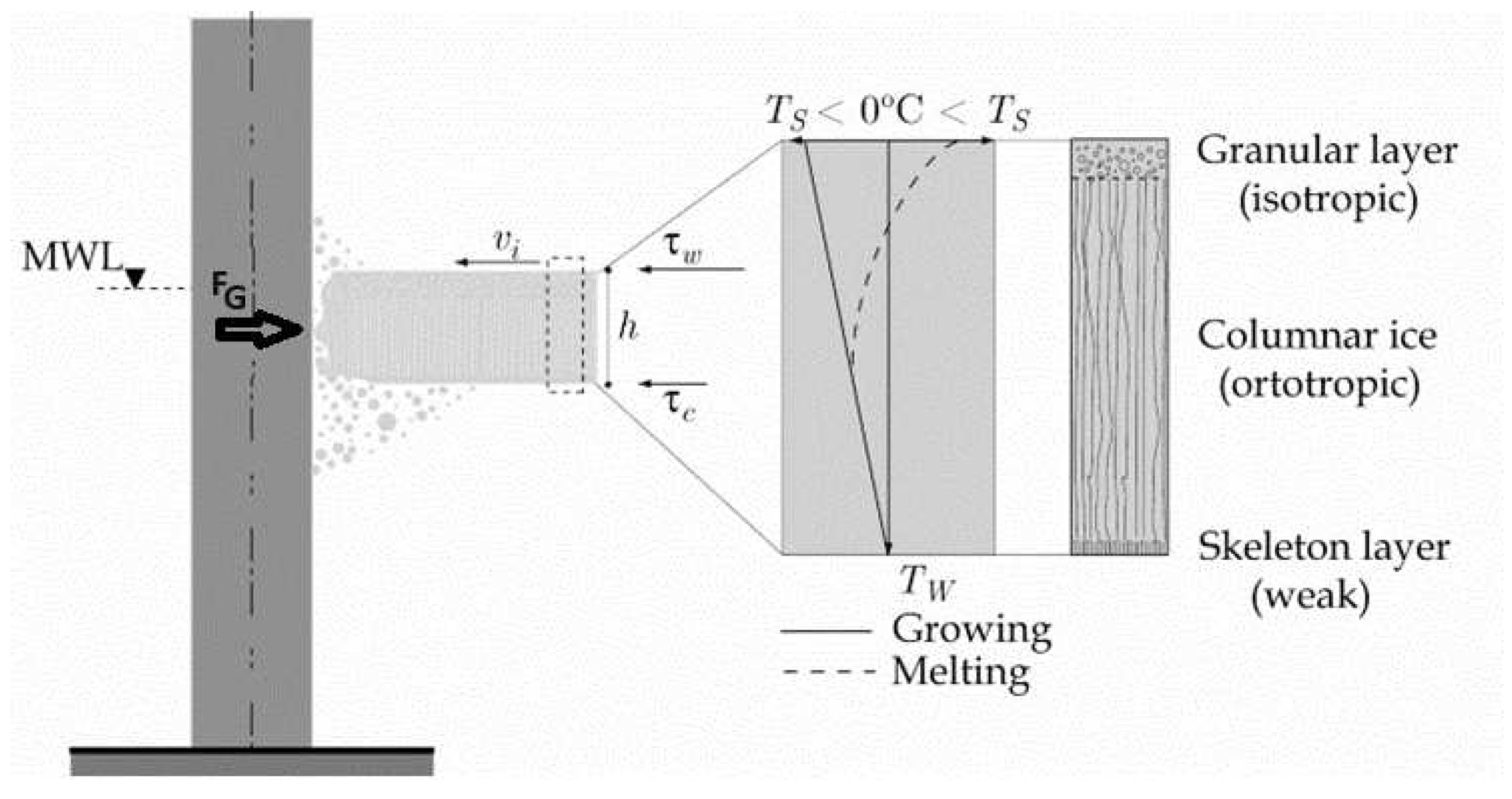
The ice-crushing failure mechanism typically occurs when ice interacts with a vertical structure. The ISO 19906 standard specifies the ice pressure (PG) and the global ice load (FG) in Equations (1) and (2). Crushing against a vertical structure, which is perpendicular to the contact surface, is referred to as the limit mechanism, as illustrated in Figure 1.
where h is the ice thickness and h1 is a reference thickness. It is typically assigned as 1 m. CR is the ice strength coefficient, w is the width of the structure, n is an empirical coefficient equal to (−0.5 + h/5) for h < 1.0 m and equal to −0.30 for h ≥ 1.0 m, and m is an empirical coefficient equal to −0.16 [4]. The analysis includes different structural widths, namely 1 m, 4 m, and 10 m. This investigation is part of a probabilistic assessment using Monte Carlo simulation.

Figure 1.
A vertical-sided structure under sea ice action (side view). MWL: Mean Water Level, Ts: Surface temperature, Tw: Water temperature, vi: ice drift velocity, τw: Air stress [The force per unit area exerted by the wind on the surface], τc: Water stress [The force per unit area exerted by the water on the bottom surface].
2.2. Sloping Structures
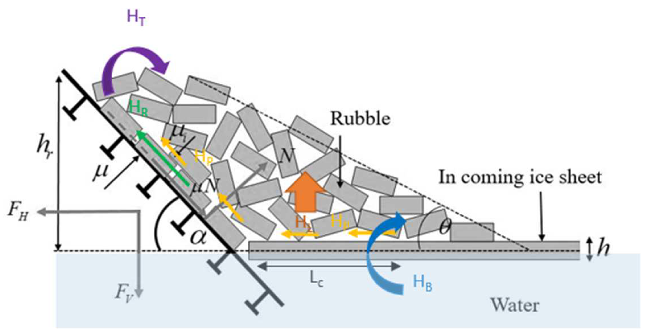
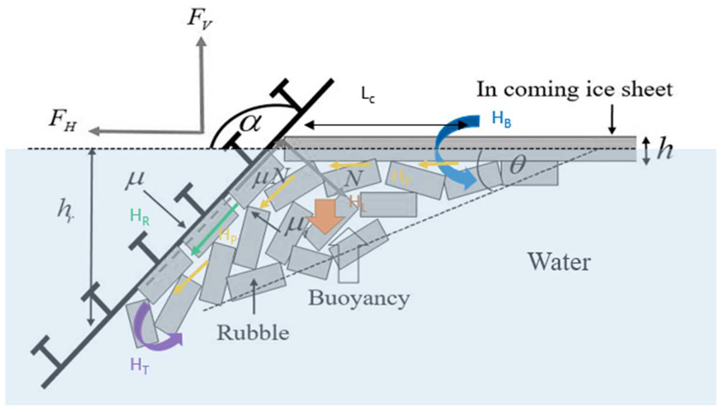
The primary emphasis of this study is on evaluating ice loading through the application of the formula prescribed by the ISO 19906 standard, which is grounded in the theoretical framework of elastic beam bending on an elastic foundation [4,12]. Inclined slope configurations can be categorized into two primary groups, depicting upward and downward slopes as depicted in Figure 2 and Figure 3, respectively.

Figure 2.
Ice–structure interaction with upward slope.
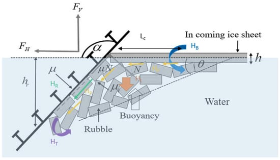
Figure 3.
Ice–structure interaction in the case of a downward slope.
For downward-sloping structures, the weight of ice fragments or rubble resulting from ice sheet fractures is treated as submerged weight, accounting for buoyancy effects.
The principal constituents of the global ice loads can be segregated into horizontal and vertical components. These components are upon the normal force (N) exerted by the ice on the structure, the angle of inclination (α), and the friction coefficient (μst) characterizing the roughness interface between sea ice and the structure. Equations (3) and (4) delineate the mathematical expressions for the horizontal ice force (FH) and vertical ice force (FV), respectively.
The loading ratio (ξ) derived from the horizontal and vertical ice load components is formulated in Equation (5).
In the ISO 19906 standard, the horizontal global ice load is categorized into five components based on the interaction mechanism.
These include:
- Breaking load (HB).
- The load component required to push the sheet ice through the ice rubble (HP).
- The load required in order to push the ice blocks up the slope through the ice rubble (HR).
- The load required to lift the ice rubble on top of the advancing ice sheet prior to breaking it (HL).
- The load needed to turn the ice block at the top of the slope (HT).
This formulation is expressed by means of Equation (6).
where lc represents the total length of the circumferential crack. The breaking load component (HB) is the primary load factor, involving the bending of the ice sheet and influencing its flexural strength, σf This relationship is expressed as follows:
Here, ρw represents the density of seawater, g denotes gravitational acceleration, and w signifies the width of the structure. In ice–structure interactions, the length of the ice sheet from the interaction zone to the fracture location is termed the critical length (Lc). The theoretical expression for the critical length is derived from elastic plate bending, represented by Equation (8):
Here, E represents the elastic modulus and ε denotes the Poisson ratio.
To facilitate the movement of the advancing ice sheet through the ice rubble, the load component Hp emerges, formulated as follows:
Here, hr stands for the rubble height, μ denotes the friction coefficient between ice-to-ice rubble, ρi represents the density of sea ice, and θ signifies the angle that the rubble forms with the horizontal plane.
The extra force needed to push the ice blocks uphill through the ice rubble is represented by the load component HR, defined in Equation (10):
The parameter P is formulated by Equation (11).
Equation (12) provides the formulation for the load component HL.
Here, c represents the cohesion of the ice rubble, and ϕ denotes the corresponding friction angle. The load component HT arises from the rotation of the ice block at the slope’s summit, as described by Equation (13).
During the interaction between ice and the sloping structure, the accumulation of ice fragments substantially enlarges the extent of the rubble pile’s ride-up. Empirical formulas derived from data collected at the Kemi-I Lighthouse and the Confederation Bridge are employed to calculate the height of the rubble pile [13]. The elevation of ice ride-up or rubble pile-up correlates with the water level or the level of the ice surface. At the Kemi-I Lighthouse, the height of rubble pile-up exhibits a linear increase, detailed in Equation (14). Meanwhile, at the Confederation Bridge, the rubble pile-up height adheres to a power law function, as specified in Equation (15).
2.3. Ice Load on Vessel Station-Keeping
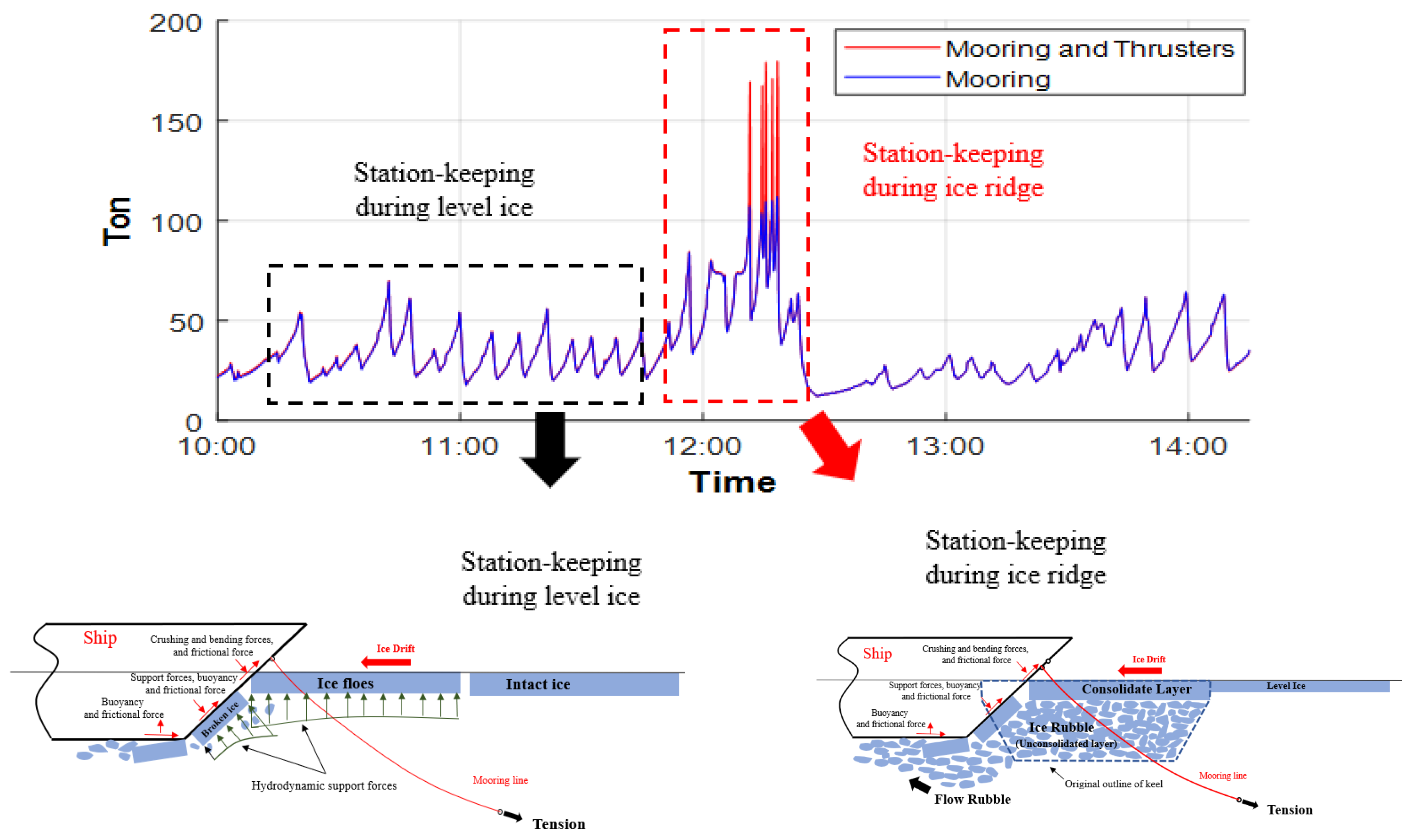
The temporal fluctuations in mooring line tension are intricately tied to the dynamics of ship–ice interactions. Estimating the cumulative ice-induced loads on the vessel during station-keeping involves employing the resistance method. This method, often referenced in the ice mechanics literature [14], serves to characterize the comprehensive ice loads arising from the interaction between the vessel and ice and to compute the propulsive force necessary for ships navigating through sea ice [15]. For stationary vessels, the method substitutes ice drift speed [16] for relative ship speed to gauge total mooring loads. The resistance method encompasses the summation of forces originating from two primary mechanisms [17]: level ice resistance and ridge resistance, depicted in Figure 4.
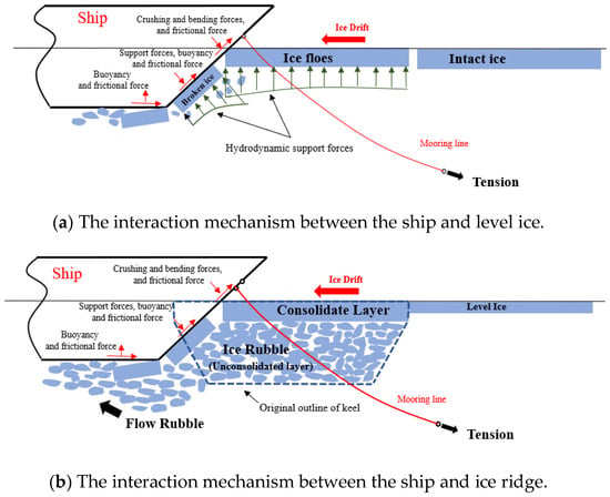
Figure 4.
Illustrates the processes of ice and ship interaction mechanisms.
The total ice load, Fice(t), on the vessel comprises the level ice component at the bow, Fi(t), the ridge component at the bow, Fb(t), and the ice load on the midship area due to the ridge rubble, Fm(t), and is defined by Equation (16). Currently, hydrodynamic loading is neglected, as it is considered minor compared to ice loading during the station-keeping experiment [17].
Fi(t) represents the resistance component due to the breaking of level ice, which can be computed using the ice resistance method developed by Riska [14]. Riska derived a simplified expression based on foundational formulations by Kämäräinen [18], Ionov [19], and Lindquist [20]. The expression by Riska [14] was calibrated using data from full-scale experiments conducted on ten Finnish merchant vessels with Baltic ice classes operating in the same region. Level ice resistance is assumed to be linearly dependent on ship speed, as depicted in Equation (17).
The coefficient C1(t), which varies with speed, and the coefficient, C2(t), which is independent of speed, are defined by Equations (18) and (19), respectively.
The variables hi, B, L, Lb, Lm, and ϕ represent the level ice thickness, ship breadth at waterline, ship length at waterline, ship length at bow entrance, ship length at midship parallel, and stem angle, respectively. The parameters f1, f2, and f3 are 230, 4580, and 1470 N/m3, and g1, g2, and g3 are 1890 N/(m2.5/s), 670 N/(m3/s), and 1550 N/(m3.5/s) [14].
The ridge resistance component is calculated using the method of Mellor [21], which applies Rankine’s plasticity model to characterize the ridge rubble as a cohesive-less continuum material. The material’s plastic behavior is characterized by the internal friction angle ϕ. Equation (20) expresses the resistance component [20,22] due to displacing the ridge keel at the bow section.
where hr represents the local ridge thickness, ψ is the normal angle to horizontal at the bow, and Cp is a constant determined by the internal friction angle of the ridge rubble, as defined in Equation (21).
where the parameter ρΔ signifies the density disparity between seawater and ice. p denotes the porosity of the ridge, typically ranging from 0.25 to 0.4, while the internal friction angle ϕr varies between 47 and 58 degrees. Sea ice density ranges between 890 and 930 kg/m3, with a seawater density of approximately 1025 kg/m3 [21].
The midship resistance component Fm of Equation (16) is expressed by Equation (22) [19].
The integration is conducted over the parallel midship area, extending from the bow shoulder to the stern shoulder (i.e., Lm), and the term (hr(x)/T – 0.5)·B is included only when hr(x) > 0.5T·Cm, where Cm is a constant contingent upon Poisson’s ratio, v, for the ridge rubble, as defined by
The parameter μi represents the friction coefficient between the ship and the ice. The variable g denotes the acceleration due to gravity. Poisson’s ratio, v, ranges between 0.21 and 0.3. The limit depth of ridge keels for the Baltic Sea can be estimated using the method proposed by Hopkins, Hibler III, and Flato [23], as described in Equation (24).
2.4. Detection of Load Peaks in Measured Data
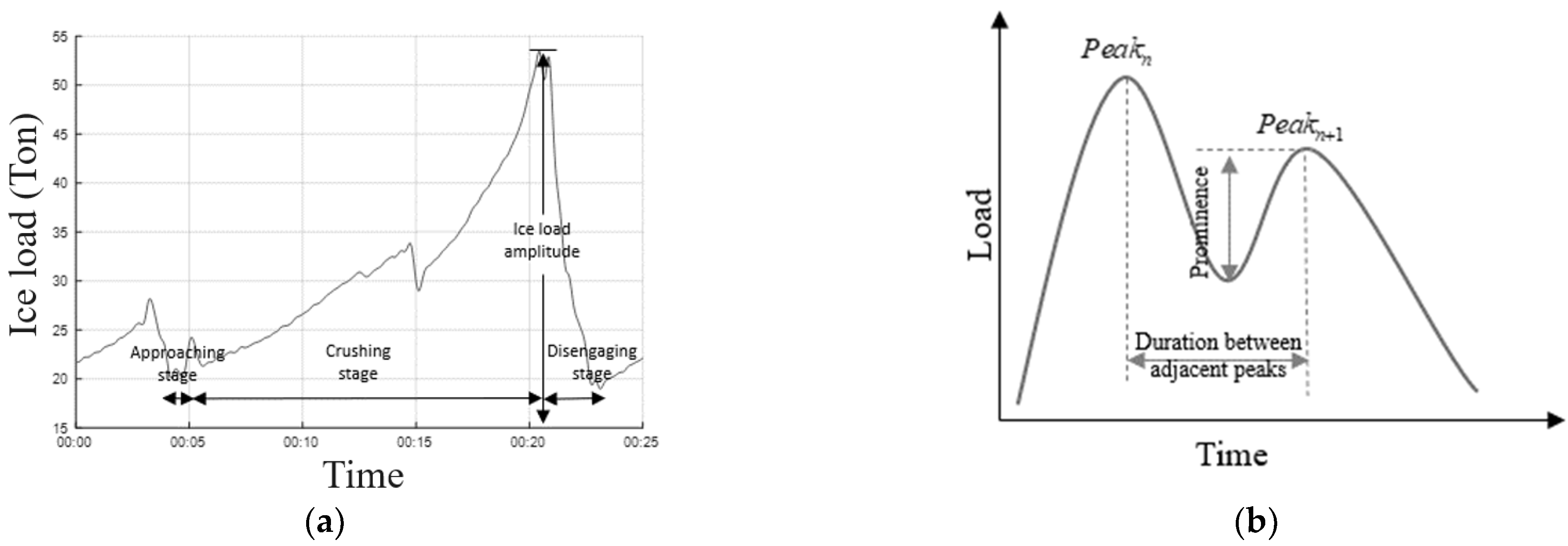
The time series data of measured ice-induced mooring loads typically exhibit a sequence of sharp peak impulses. The process of ice-induced loading is characterized by three distinct stages: approach, crushing, and disengagement. During the full-scale experiments, the ice concentration was exceptionally high, reaching approximately 9.5 out of 10. In cases of peak ice concentration, the approach stage of the ice-induced mooring load is very brief, as depicted in Figure 5a. This three-stage pattern of mooring load persists continuously as the ship hull encounters successive ice edges.

Figure 5.
(a) Illustration of the three stages involved in the ice load generation process. (b) Visualization of the process for detecting peaks using prominence.
The peaks in mooring line tension are identified using the peaks prominence method implemented in a Matlab 2020 toolbox. This method is based on measuring the shortest vertical distance from each peak to the lowest neighboring valley. Its application helps exclude small peaks resulting from signal noise in the recorded time series. Figure 5b demonstrates a sequence of peak detections using this method.
3. Probabilistic Assessment
The probabilistic assessment methodology concerning ice–structure interactions initiates by scrutinizing foundational ice data specific to the site -, including parameters such as ice thickness, ice strength coefficient, and flexural strength. These essential ice datasets are then subjected to fitting with probabilistic models. In this study, a spectrum of correlation coefficients, ranging from minimum to maximum values, is applied in conjunction with the Nataf model. Monte Carlo simulation (MCS) techniques are subsequently employed to generate comprehensive samples of random variables for the key parameters.
3.1. Monte Carlo Simulation
Monte Carlo simulation (MCS) is employed to conduct a probabilistic assessment of the loads induced by ice–structure interactions. For vertical structures, the simulations involve varying ice thickness and ice strength coefficient values to examine uncertainties associated with horizontal ice pressure and overall ice loads. In contrast, for sloping structures, the simulations focus on the flexural strength values of sea ice instead of the ice strength coefficient. The values for level ice thickness, xi, flexural strength, xj, and the ice strength coefficient, xk, are generated using the inverse cumulative distribution function (CDF) of the Normal distribution and Weibull distribution, respectively. These sample values are derived from random numbers drawn from a uniform distribution, xu, denoted by U(0,1). The specific sample values are expressed by Equations (25)–(27) below, with the current sample size set at n = 10,000.
This study also explores the implications of introducing correlations between the principal parameters. In vertical structures, these parameters involve the ice thickness and ice strength coefficient, whereas in sloping structures, they encompass the ice thickness and flexural strength.
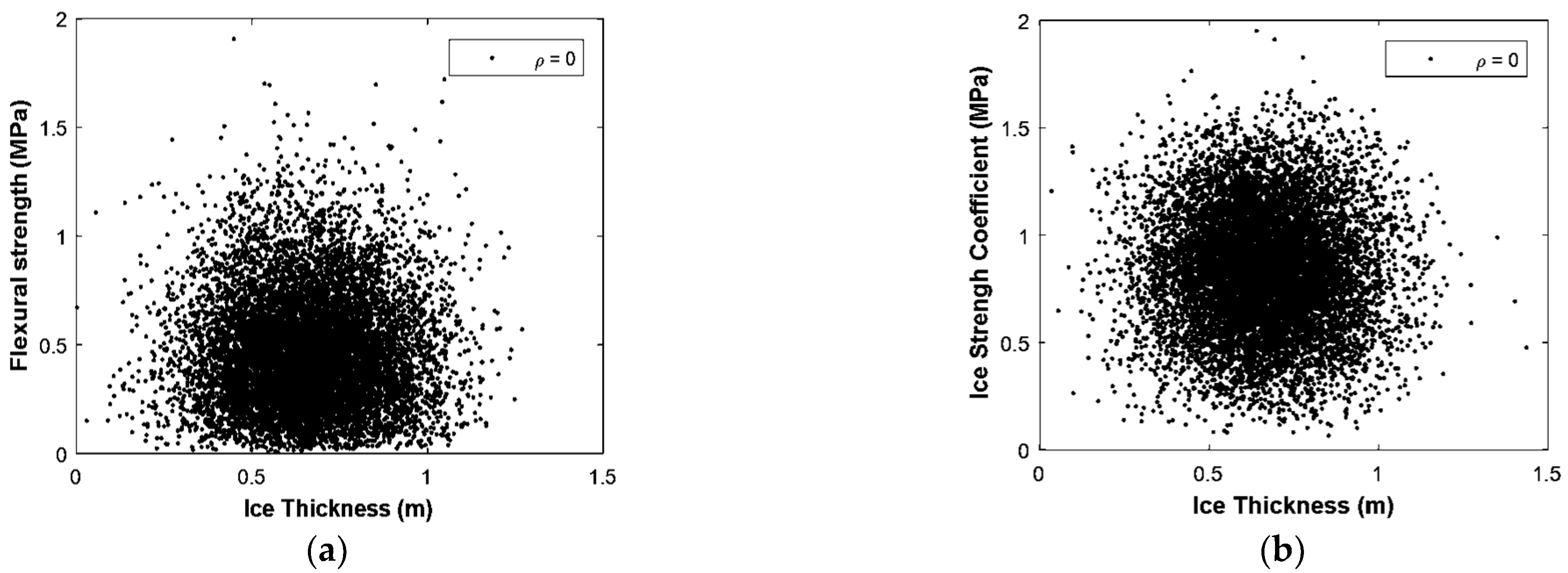
The condition of independence among the fundamental variables is characterized by setting the correlation coefficient ρ to zero, which serves as the initial input for the MCS. The scatter plot depicting the independent relationship between ice thickness and flexural strength for sloping structures is depicted in Figure 6a. Similarly, the scatter plot illustrating the independent relationship between ice thickness and the ice strength coefficient for vertical structures is shown in Figure 6b. Subsequently, the study explores the effects of introducing correlations between these variables using the NATAF transformation model.
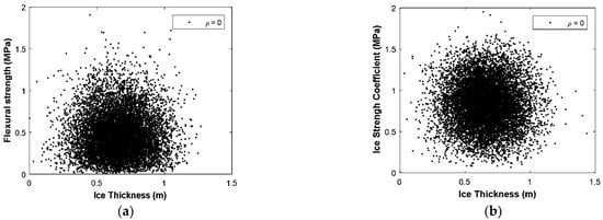
Figure 6.
Demonstration of independent samples using MCS: (a) ice thickness and flexural strength and (b) ice thickness and ice strength coefficient.
3.2. NATAF Transformation Model
Typically, there is a correlation between the parameters that characterize the physical properties of sea ice. This correlation can be estimated using experimental data. The NATAF transformation model is capable of representing this correlation structure to generate the associated joint probability density and distribution functions [24]. The fundamental assumption of the NATAF transformation model is that the basic random variables representing the physical properties of sea ice can be derived by transforming the corresponding Gaussian variables zi, zj, zk and vice versa, as described by Equations (28)–(30).
The correlation coefficient ρ0,ij between the two Gaussian variables zi and zj is related to the correlation coefficient ρij between the thickness xi and flexural strength of sea ice xj. The correlation between the random variables representing the physical parameters, i.e., xi and xj, is given by:
where E(xr) = μr, , r = i, j, or r = i, k; and φ2 is the bivariate standard normal probability density function as defined in Equation (32).
In the Gaussian plane, the uncorrelated variables zi and zj can be converted into correlated variables and , as specified in Equation (33).
For vertical structures, the parameter xk, representing the ice strength coefficients in Equations (28) and (29), is employed in lieu of the flexural strength of sea ice, xj. The NATAF transformation model remains valid across the entire spectrum of the correlation coefficient (i.e., from −1 to 1). This study investigates the influence of the correlation between key parameters of ice loading on vertical and sloping structures. Five distinct values for the correlation coefficient ρ are utilized: [−0.9, −0.5, 0.0, 0.5, 0.9], encompassing the full range from minimal to maximal values. The extreme correlation coefficient values are confined to −0.9 and 0.9 due to numerical constraints inherent in the transformation process (i.e., the transformation matrix in Equation (33) becomes singular as the absolute value of the correlation coefficient nears 1.0).
3.3. Implementation of Extreme Value Analysis
The extreme mooring loads for each ice management scheme are estimated based on full-scale measurements. The observed peak mooring loads at the Magne Viking (MV) are treated as random variables for analysis. The sample values of tension peak loads, denoted as t1,…,tN, are assumed to be independent realizations from the same underlying probability distribution, F(t), which is used to establish the extreme value distribution. The probability distribution for the maximum mooring load, η, corresponding to a sample size N, is given in Equation (34).
Assuming the sample values are independent and identically distributed, Equation (34) can be simplified as shown in Equation (35).
Here, N represents the count of ice load peak events during the specified period for each ice management scheme.
3.3.1. The Peaks-over-Threshold and Block Maxima Methods
In this investigation, two established methodologies are employed to forecast extreme loads: the peaks-over-threshold (POT) and block maxima (BM) methods. Initially proposed by [25], the POT method entails identifying peaks in mooring line loads that surpass a specified threshold, facilitating the fitting of an initial distribution, F(t). The non-exceedance probability is determined under the no-bias condition [26], indicating the occurrence of n peaks out of a total NTotal, as detailed in Equation (36).
For the BM method, the peak mooring load values within a fixed-duration time window are initially fitted with a suitable distribution model. This fitted distribution is then utilized in Equation (36) to derive the extreme value distribution. The extreme value corresponding to a specified exceedance probability, λ, is subsequently determined using Equation (37).
Here, the exceedance probability level λ aligns with a specific return period, as defined by Equation (37). Furthermore, NBox represents the division of the measurement record into blocks. Figure 7 depicts the respective peak values utilized in both POT and BM methodologies.

Figure 7.
Illustration of the POT and BM methods. (a) Peaks-over-threshold method (POT). (b) Block maxima method (BM).
To forecast the short-term extreme mooring load during the full-scale experiment, the exceedance probability λ, linked to a specific number of operational repetitions, can be derived from the return period relative to the total days under consideration, Tday (such as the number of days in a year). This relationship is expressed as follows:
Here, Ttest denotes the duration of a specific full-scale test. In this context, R represents a reduction factor indicating the proportion of time relative to Tday during which the operation is conducted. For estimating extreme values, the Gumbel distribution is commonly utilized as the initial model, primarily because it is assumed to be the appropriate asymptotic distribution for the given scenario, with little additional justification typically provided. The cumulative distribution function (CDF) and the probability density function (PDF) of the Gumbel distribution are expressed by Equations (39) and (40), respectively:
The parameters β and α represent the location and scale of the Gumbel distribution. These parameters can be determined, for instance, through methods such as least squares fitting on probability paper, method of moments, or maximum likelihood estimation. Additionally, the scale parameters of the BM method can be related to the scale parameters of the POT method, as shown in Equation (41).
3.3.2. The ACER Method
The ACER method provides a computational framework suitable for investigating extreme mooring loads across various ice management strategies. One of its key advantages is its capacity to function as a robust diagnostic tool, allowing for the verification of the inherent extreme value distribution within sampled datasets. This approach generates a nonparametric representation of the distribution, enabling an assessment of the applicability of asymptotic distributions commonly used in analyzing extreme value data extracted from time series. A fundamental aspect of the ACER method involves the sequence of ACER functions [26], which vary in order k and converge towards the extreme value distribution inherent in the data as k increases. It is adaptable for analyzing both stationary and non-stationary datasets of stochastic processes. For a more detailed exploration of the principles and advancements in extreme value estimation using the ACER method, comprehensive discussions can be found in Naess and Gaidai [27] and Naess, Gaidai, and Karpa [28]. Further guidance on employing the ACER method for data analysis is available in Naess, Gaidai, and Karpa [28], where Equation (42) defines the formulation of the target probability distribution for extreme value analysis using this method.
The symbol represents the empirical ACER function of order k, estimated from the dataset where N denotes the total number of data points in the sampled time series. Generally, increasing the order k of the ACER function enhances accuracy, although the optimal k value for precise estimation heavily relies on the dependence structure within the time series. In cases of independent data, k = 1 suffices. For dependent data, a reasonable engineering approximation is achieved with k = 2 aligning with the classical Poisson assumption of independent upcrossings at high response levels. For extrapolating data akin to that examined in this study, the ACER functions are approximated using the following set of parametric functions:
The coefficients ak, bk, ck and qk are constants that vary with the order k, and η0 represents a threshold beyond which Equation (43) is deemed applicable. The coefficients ak, bk, ck and qk are constrained to ak > 0, bk ≤ η0 and ck > 0. It is noteworthy that for this set of parametric functions, the underlying asymptotic extreme value distribution conforms to the Gumbel type, where ck = 0. However, when fitting these functions to actual data, which typically do not exhibit asymptotic behavior, the parameter ck seldom equals zero. Thus, assuming the asymptotic Gumbel distribution for extremes in such scenarios would be questionable. In this study, we employ the ACER method specifically to evaluate the validity of this assumption for our dataset.
4. Case Study
4.1. Probabilistic Assessment of a Fixed Offshore Structure under Ice Loading
In this section, the outcomes of analyzing ice loads on structures using the ISO standard are presented. The approach to analyzing ice load differs between vertical and sloping structures primarily because the failure mechanisms of sea ice vary between the two cases: crushing mode for vertical structures and flexural mode for sloping structures.
4.1.1. Vertical Structures
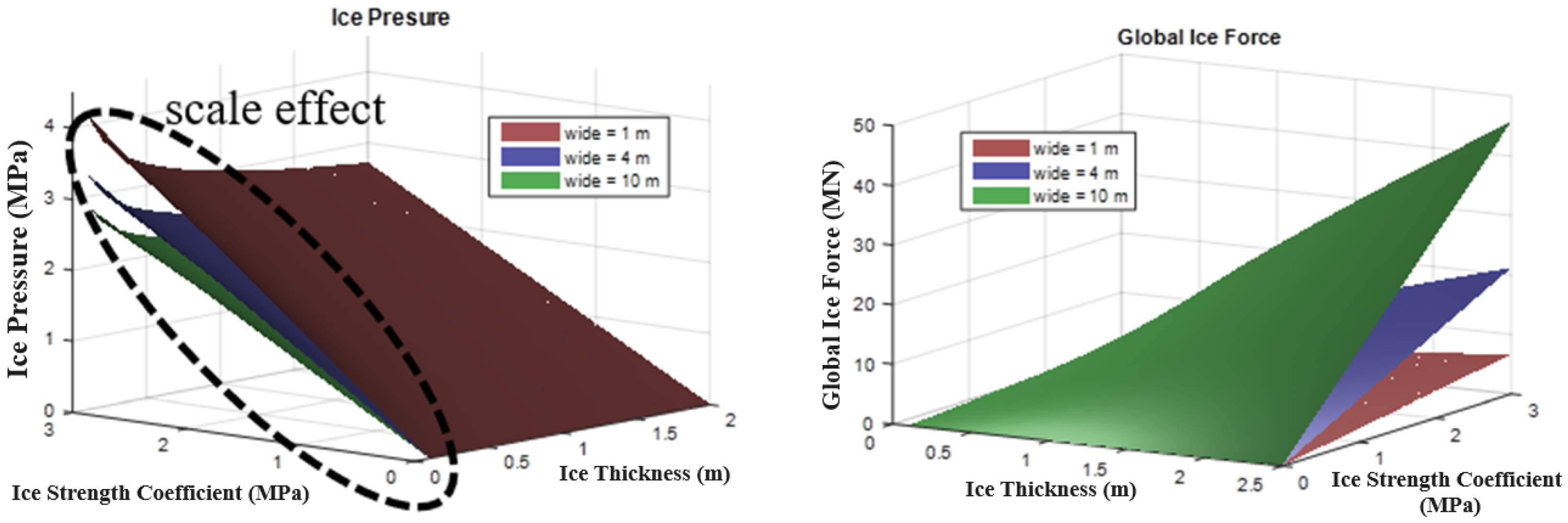
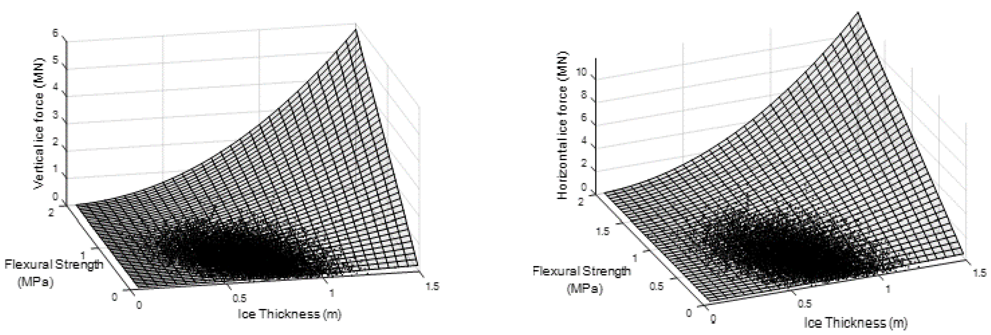
As part of the probabilistic assessment, the Normal distribution and the Weibull distribution are found to provide suitable fits for the level ice thickness and ice strength coefficient. The parameters μ (mean) and σ (standard deviation) for the Normal distribution are 0.662 m and 0.175 m, respectively. For the Weibull distribution, these parameters (shape and scale) are determined as 4.504 and 0.446, respectively [6]. The uncertainty in ice loading on vertical structures considers only the statistical variability of the level ice thickness and ice strength coefficient, excluding uncertainties due to the exponents n and m in Equation (1). The ice pressure and global ice force, as defined by ISO standards, are presented in Figure 8. The influence of correlation between ice thickness and ice strength coefficient on ice pressures and global ice forces is investigated using the NATAF transformation model. Numerical samples based on the NATAF transformation model for a correlation coefficient of −0.5 are depicted in Figure 9, showing data points where scale effects are significant. More negative correlation coefficients tend to result in more data points in regions where scale effects are notable, although these points do not correspond to high values of global ice force.

Figure 8.
Illustrates how average ice pressure and global ice loads change with varying structural widths, as functions of ice thickness and ice strength coefficient [6].
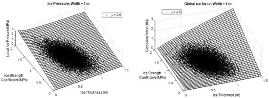
Figure 9.
Examples of average ice pressures and global ice forces utilizing the NATAF transformation model with ρ = −0.5 and w = 1 m.
Samples generated through MCS are utilized to fit distributions, enabling a detailed examination of the statistical properties of global ice loads. Figure 10 illustrates an example plot demonstrating the fitting of the Weibull distribution to characterize the average ice pressure and global ice forces exerted on vertical structures.

Figure 10.
Illustration of linear regression applied to fit average ice pressure and global ice forces for a vertical structure using the Weibull distribution approach (ρ = −0.5 and width = 1.00 m). (The independent variable, x, represents ice pressure (in MPa) or global ice force (in MN)).
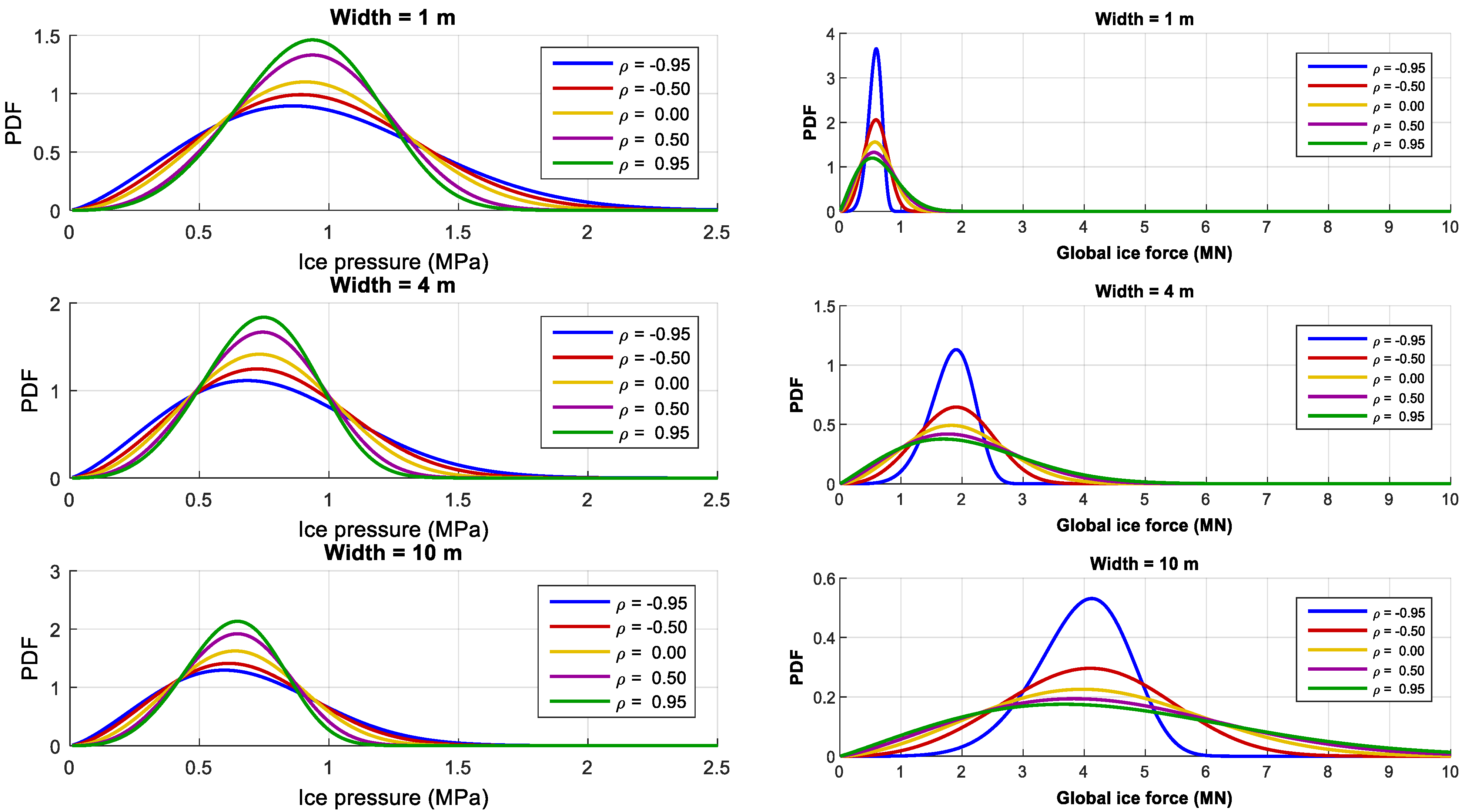
The correlation coefficient between ice thickness and the ice strength coefficient tends to flatten the shape of the average ice pressure probability density function, indicating increased uncertainty. Conversely, for global ice forces, a decrease in the correlation coefficient leads to narrower probability density functions. Figure 11 presents the Weibull probability density functions (PDFs) of ice pressure and global ice loading across various correlation levels and structural widths.
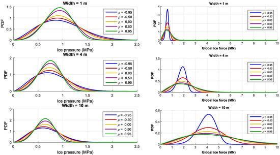
Figure 11.
Variations in the correlation levels and structural widths impact the correlations between average ice pressure and global ice loads for vertical structures, which depend on ice thickness and crushing strength.
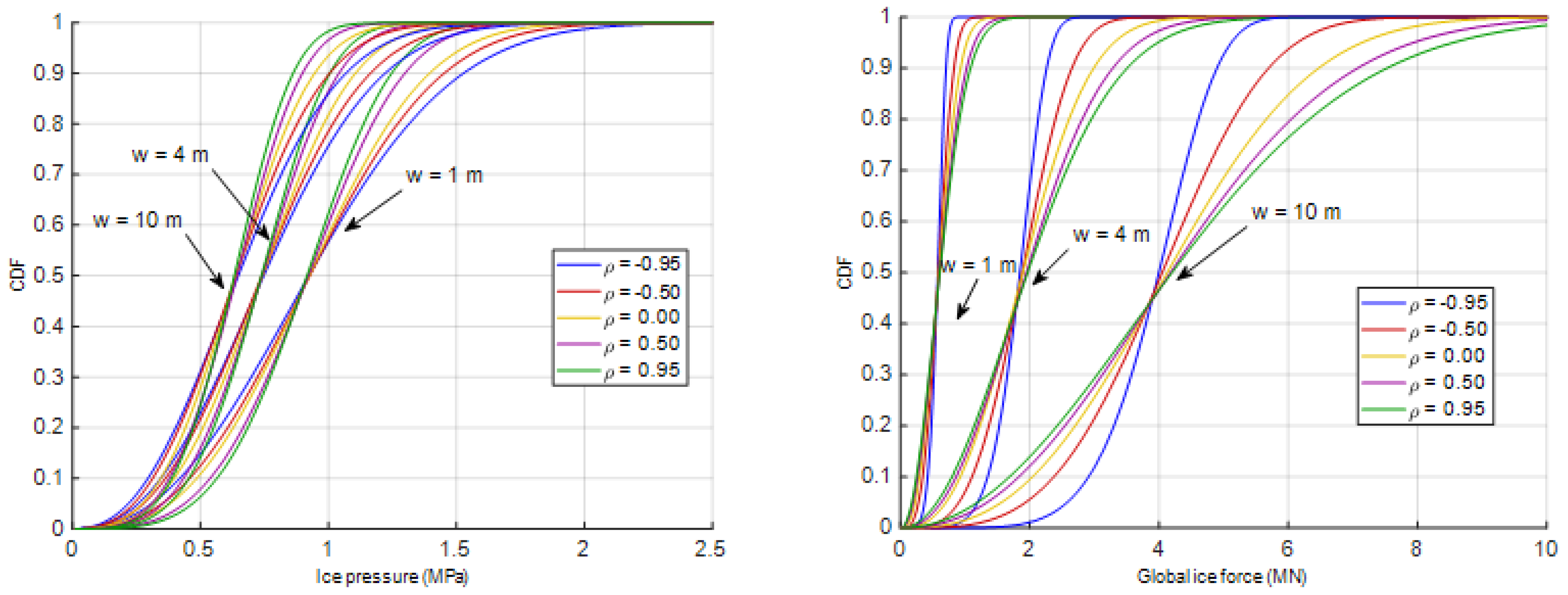
The impact of different correlation levels on the average ice pressure and global ice forces can also be examined by comparing their CDFs across various values of structural width and correlation coefficient. These trends mirror those observed in the PDFs, as depicted in Figure 12.
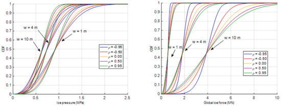
Figure 12.
The CDFs of Weibull distributions for ice pressures per square meter and global ice forces in the context of vertical structures.
4.1.2. Sloping Structures
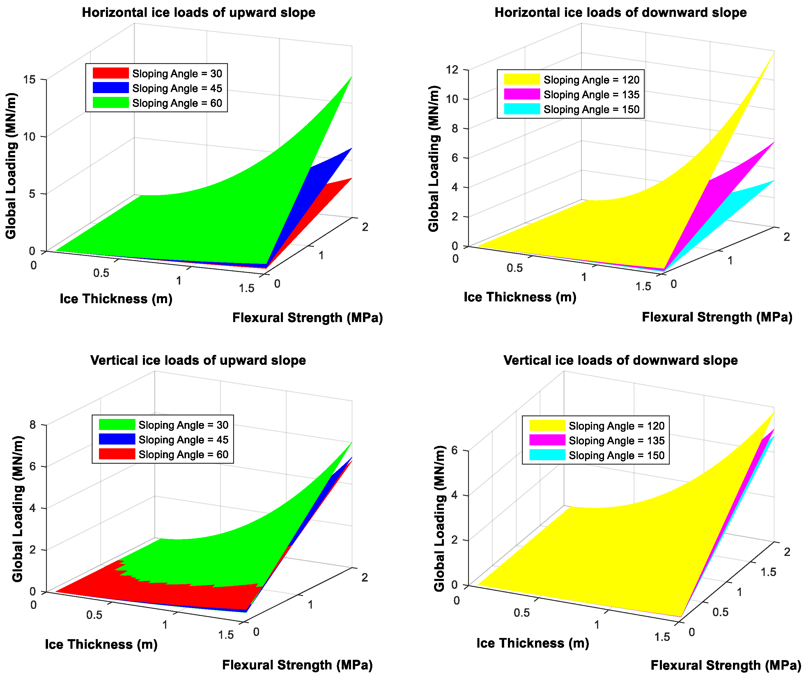
For inclined structures, according to the ISO 19906 standards (Petroleum and natural gas industries—Arctic offshore structures) [4], global ice loads show a notable increase with steeper slopes, whether upward or downward. Horizontal ice loads exhibit greater magnitudes than vertical ones, with horizontal values being more responsive to slope angles compared to vertical values, as evident in Figure 13.

Figure 13.
Ice loads in both horizontal and vertical directions on inclined structures (upward left and downward right) vary with ice thickness, flexural strength, and slope angle.
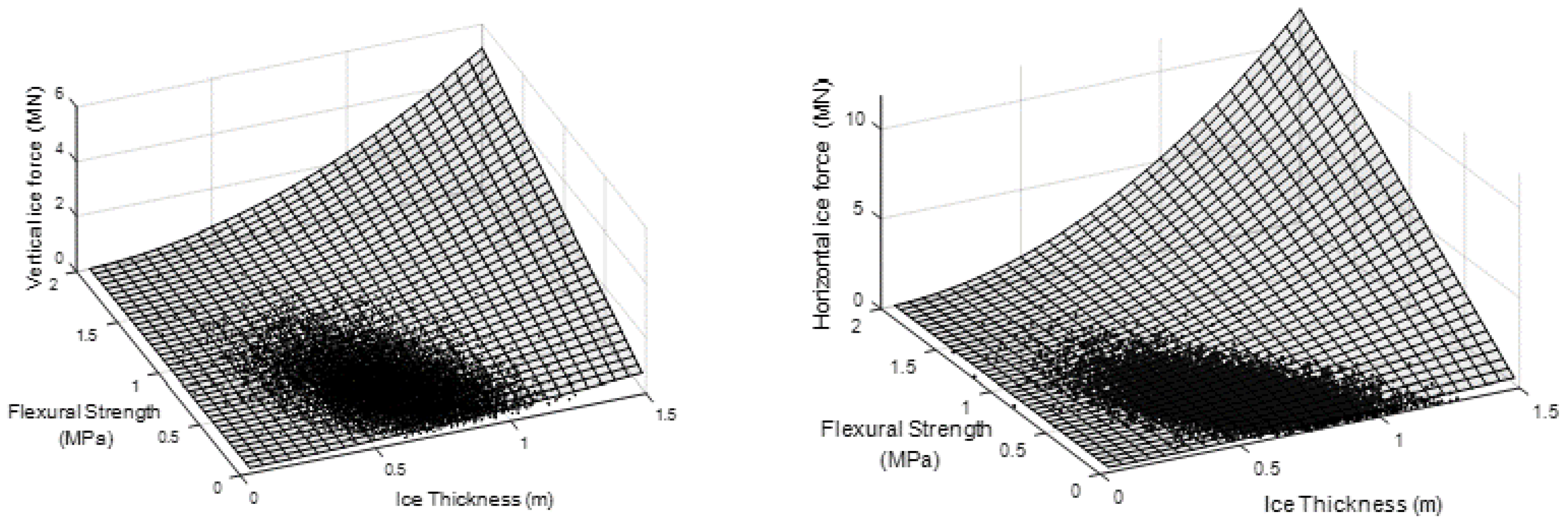
Vertical and horizontal ice load samples are created using MCS, where ice thickness and flexural strength serve as fundamental variables. These variables are then inputted into the formulas outlined in the ISO document. By employing the NATAF transformation model, the interdependence between these variables, as indicated by the correlation coefficient ρ, is taken into consideration. Scatter plots illustrating the relationships between horizontal and vertical loads for various correlation coefficients between ice thickness and flexural strength on upward and downward slopes are depicted in Figure 14 and Figure 15, respectively.

Figure 14.
Samples of the vertical and horizontal ice forces based on an application of the NATAF transformation model for ρ = −0.5 and sloping angle = 30 deg. (upwards direction).
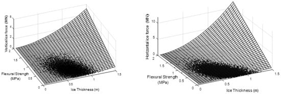
Figure 15.
Samples of the vertical and horizontal ice forces based on an application of the NATAF transformation model for ρ = −0.5 and sloping angle = 120 deg. (downwards direction).
Steeper slope geometries result in increased magnitudes and uncertainties in global horizontal ice loads. The primary contributing factor to these loads is the breaking load component HB, which involves the bending of the ice sheet and subsequent flexural failure of sea ice. Both global vertical and horizontal ice loads exhibit similar variations in trends. Generally, the mean values of ice loading show minimal change across different sloping angles. Additionally, a stronger correlation between ice thickness and flexural strength leads to greater dispersion in the PDFs, indicating higher statistical uncertainty.
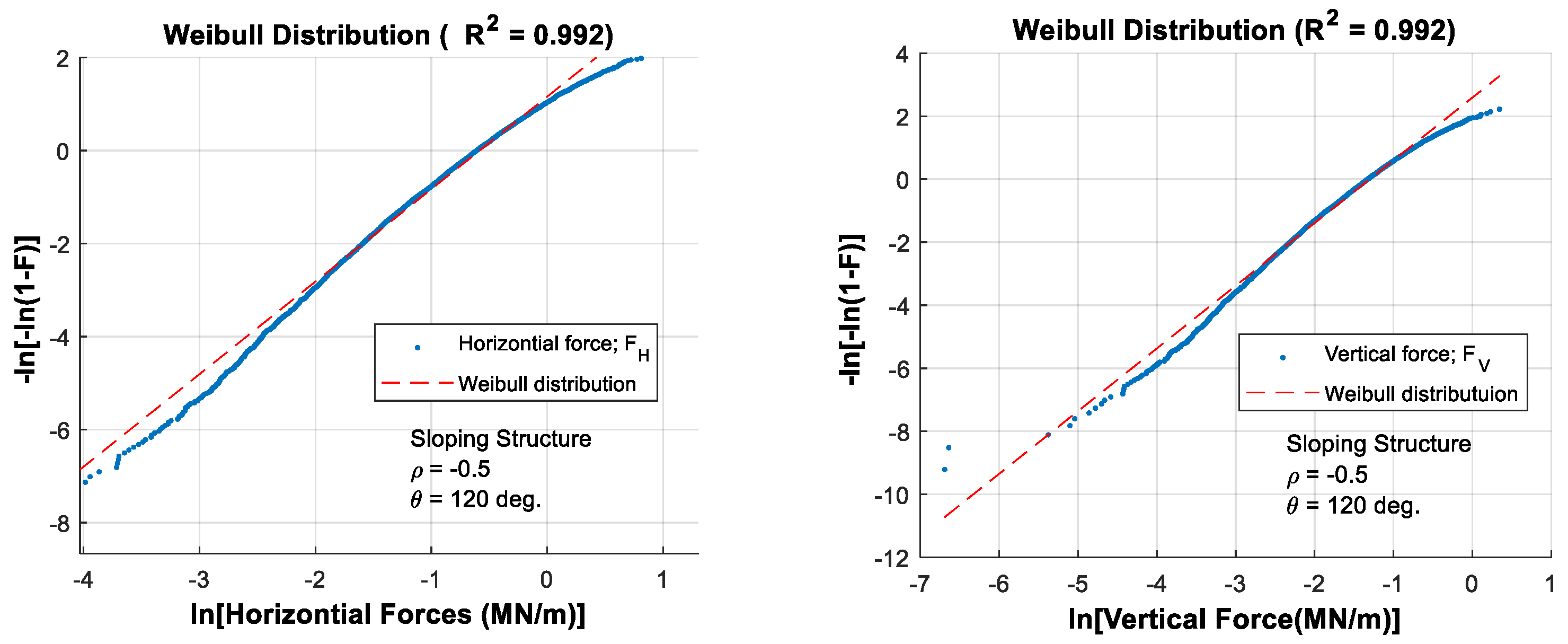
Different probabilistic models have been tested to determine the best fit for the cumulative distribution of horizontal and vertical ice forces. The analysis revealed that the Weibull distribution is the most suitable model for both components of the global ice force. Figure 16 presents examples of how the Weibull distribution fits the PDFs for horizontal and vertical ice forces.

Figure 16.
Examples of linear regression to fit the cumulative distributions of horizontal and vertical ice forces using Weibull probability paper (with a correlation coefficient of ρ = −0.5 and a sloping angle of 120 degrees).
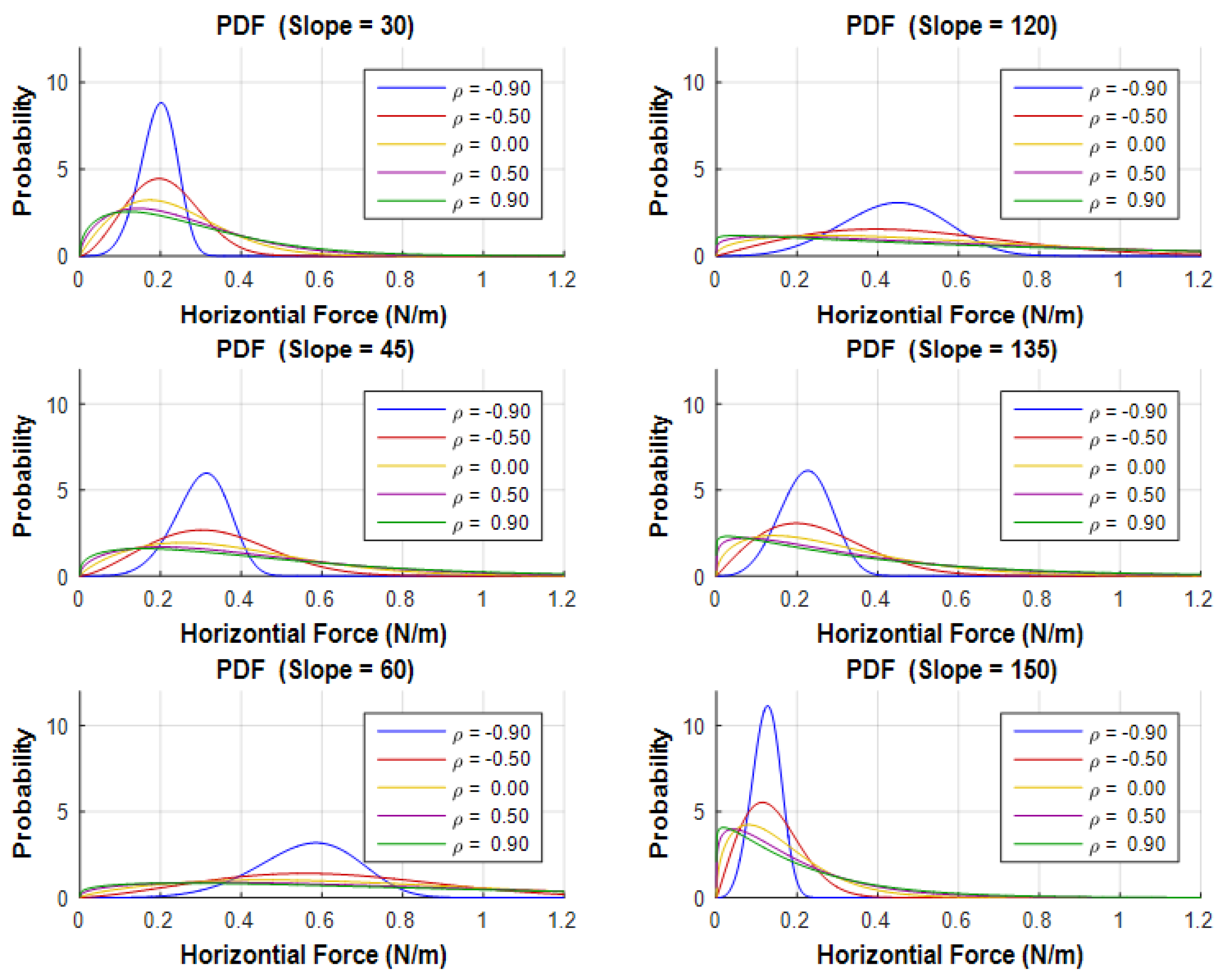
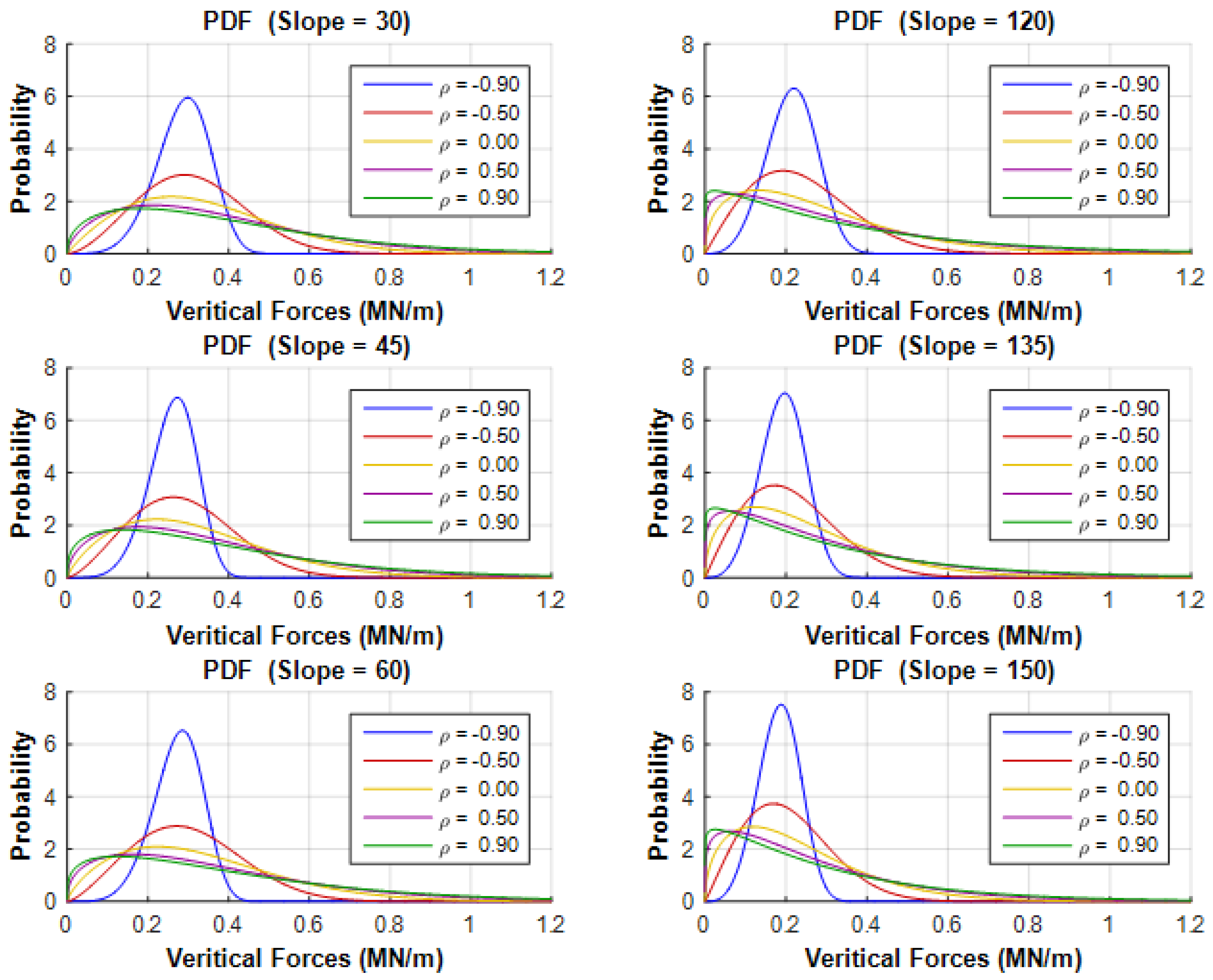
Gentler slopes lead to a notable decrease in the magnitude of horizontal loading due to a shift in sea ice failure from crushing to bending modes. The variability in global ice loads in both upward and downward directions can be discerned from the respective PDFs depicted in Figure 17 and Figure 18. These figures illustrate that the correlation coefficient between ice thickness and flexural strength significantly influences the PDF shapes, which flatten increasingly with higher correlation coefficients, observed in both upward and downward slopes.
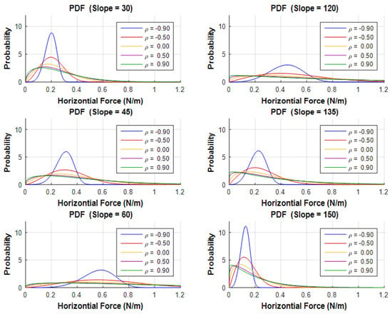
Figure 17.
PDFs based on the Weibull distribution for horizontal ice forces on inclined structures, varying with correlation coefficients and slope angles.
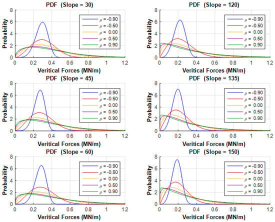
Figure 18.
Weibull probability density functions for vertical ice forces on inclined structures vary with different correlation coefficients and sloping angles.
The impact of slope angles on the uncertainty of horizontal ice loading is notable. Steeper slopes exhibit increased dispersion and uncertainty in global horizontal ice forces, as depicted in Figure 17. Conversely, slope angles have minimal influence on vertical ice forces, which is evident from the PDF shapes across various slope angles shown in Figure 18.
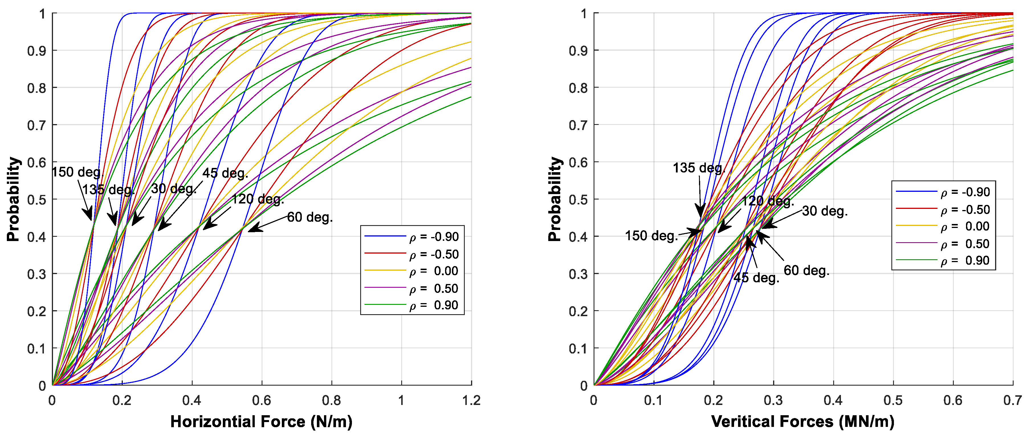
Moreover, the shapes of the CDFs in Figure 19 also depict the results of the uncertainty assessment regarding ice loading on sloping structures.

Figure 19.
Weibull cumulative distribution functions representing horizontal and vertical ice loads on sloping structures, varied across different correlation coefficients and sloping angles.
4.2. Extreme Value Analysis of Ice Loading on Fixed and Floating Offshore Structures
4.2.1. Ice Management Operations
Ice management systems are typically utilized during the operations of ships and floating structures in icy regions to mitigate ice loading [8,29]. In the current experiments, an icebreaker was deployed to break ice according to various ice management strategies. The selection of vessel types and equipment for the field experiments was based on previous experience with complex marine operations under similar conditions. Two vessels were involved in the experiments: an ice-breaking vessel and a stationary supply vessel. Both vessels have extensive operational history in Arctic conditions and are equipped with diesel mechanical shaft line systems. The vessels feature nozzle-mounted propellers, with shaft generators powering electrical tunnel thrusters and retractable azimuth thrusters in the bow [30]. Magne Viking (MV) is a standard offshore vessel with a bulbous blunt shape, as depicted in Figure 20. The bow shape of the Tor Viking (TV) vessel is optimized for icebreaking and ramming, as illustrated in Figure 21.

Figure 20.
Drawing Arrangement and photo of Magne Viking (MV).

Figure 21.
Drawing Arrangement and photo of Tor Viking (TV).
4.2.2. Ice Breaker Deployment Patterns for Ice Management
The primary objective of ice management (IM) operations is to minimize the ice load on vessels, ensuring they can maintain station and conduct offshore operations effectively. The most effective strategy for reducing ice loads involves creating a uniform channel to decrease the size of moving ice floes using an icebreaker following systematic patterns [8]. To optimize performance, these patterns can be adjusted based on factors such as the speed, thickness, and turning characteristics of incoming ice, as well as the maneuvering capabilities of the icebreaker.
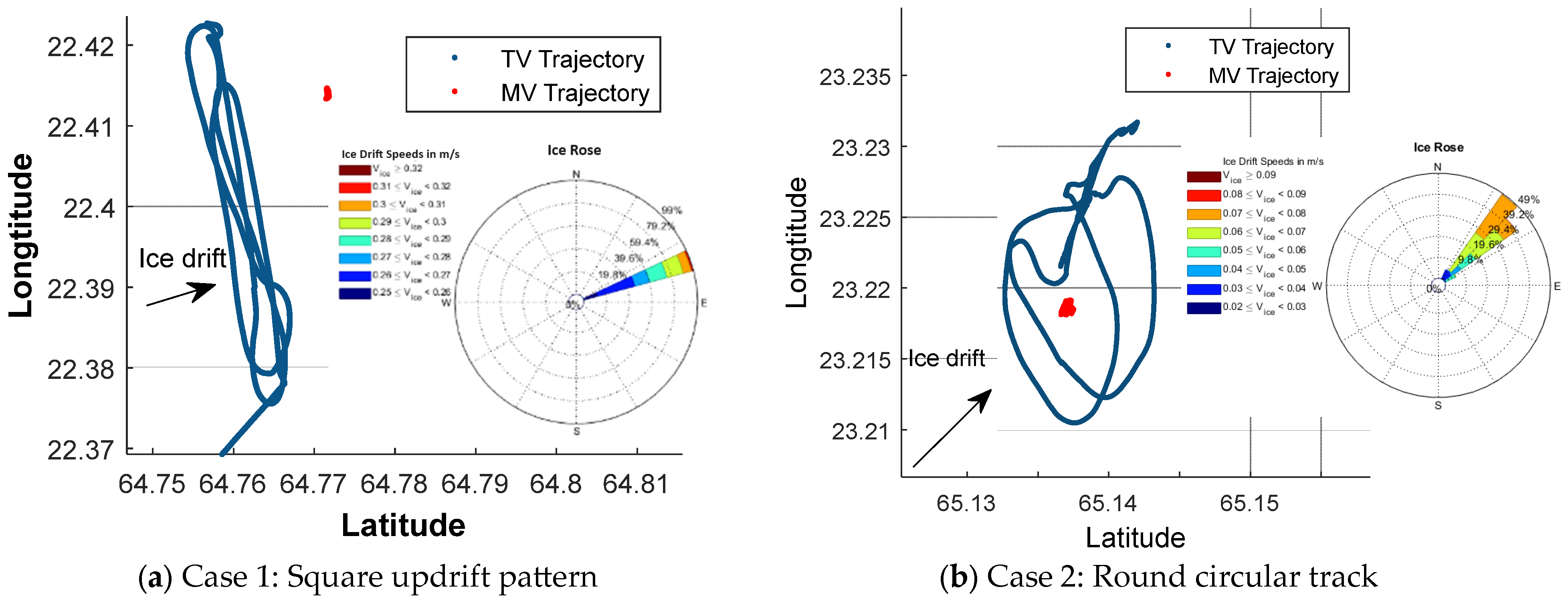
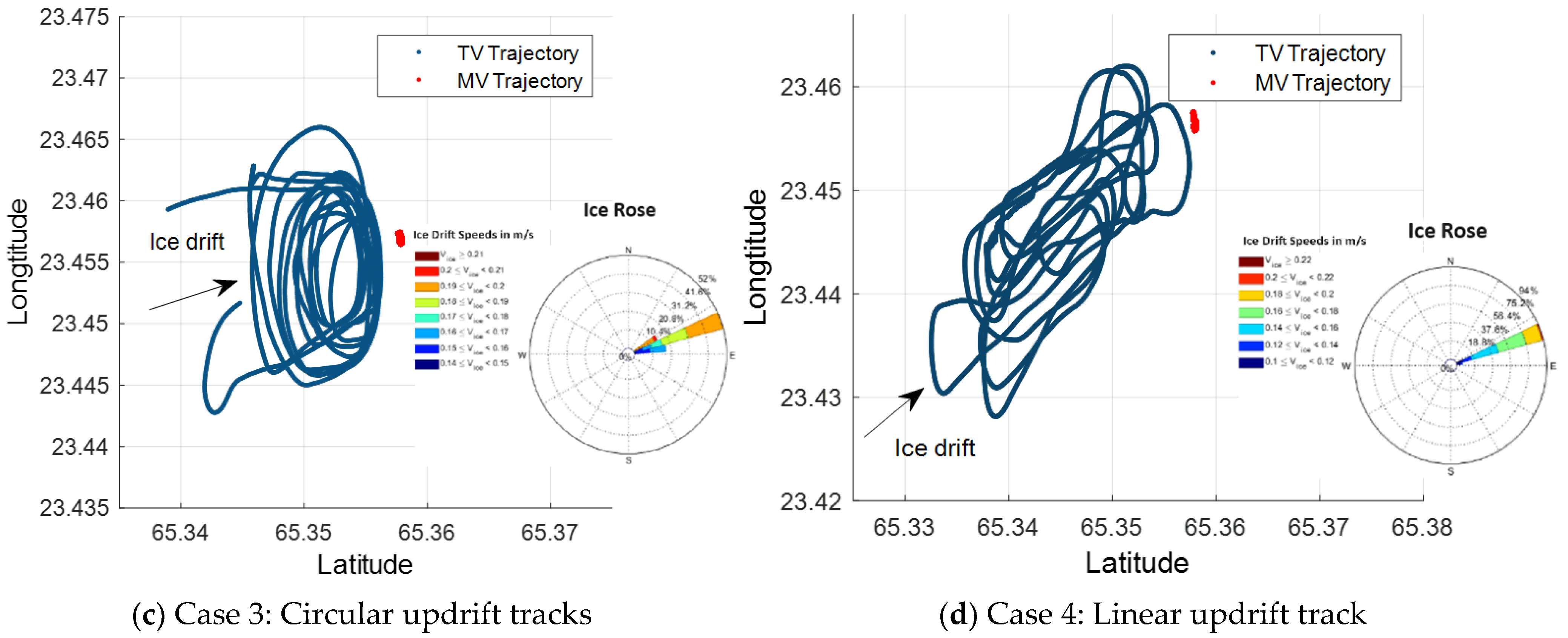
Four distinct strategies for ice management were implemented during the full-scale trials, as depicted in Figure 22. The corresponding measurement data are currently under analysis to determine the statistical characteristics of extreme mooring forces. These selected ice management patterns were planned using the ship’s Electronic Chart Display and Information System (ECDIS), which proves particularly advantageous in low-visibility conditions [31]. The most challenging aspect of ice management operations occurs during the initial pattern, primarily due to the unbroken ice at this stage. Consequently, the vessel operated at a relatively low speed during the first turn, resulting in a longer time required for the initial pass compared to subsequent maneuvers.

Figure 22.
Patterns corresponding to the different ice management schemes applied during full-scale tests.
The initial ice management scheme involves the square updrift pattern, depicted in Figure 22 (Case 1), where the icebreaker cuts through the sea ice in a straight line in the updrift direction. This pattern allows the icebreaker to gain speed along a straight path before executing sharp 90-degree turns at transition points. However, the combination of high speeds and sharp turns in the square pattern can lead to excessive vessel rolling. The second pattern is the round circular track, illustrated in Figure 22 (Case 2), where the icebreaker circles around the stationary supply vessel. This pattern is suitable for low drift speeds to minimize the size of outgoing floes and generate a large amount of brash ice. The third pattern involves circular updrift tracks, shown in Figure 22 (Case 3), which facilitate pushing ice into previously cut tracks, significantly reducing resistance during turns. The icebreaker typically achieves speeds of 10–12 knots after initiating ice management operations with this circular approach, which proves effective in most ice conditions encountered during the trials, except when ice drift speeds are high and conditions severe [31,32]. Figure 22 (Case 4) demonstrates the linear updrift track, a novel ice management scheme implemented for station-keeping trials.
The schedule of various tests is detailed in Table 1. There are slight variations compared to the originally planned mission schedule. The timings in Table 1 reflect the actual start and completion times recorded during the ice management operations.

Table 1.
The schedule for the different ice management (IM) operations.
4.2.3. Weather Conditions
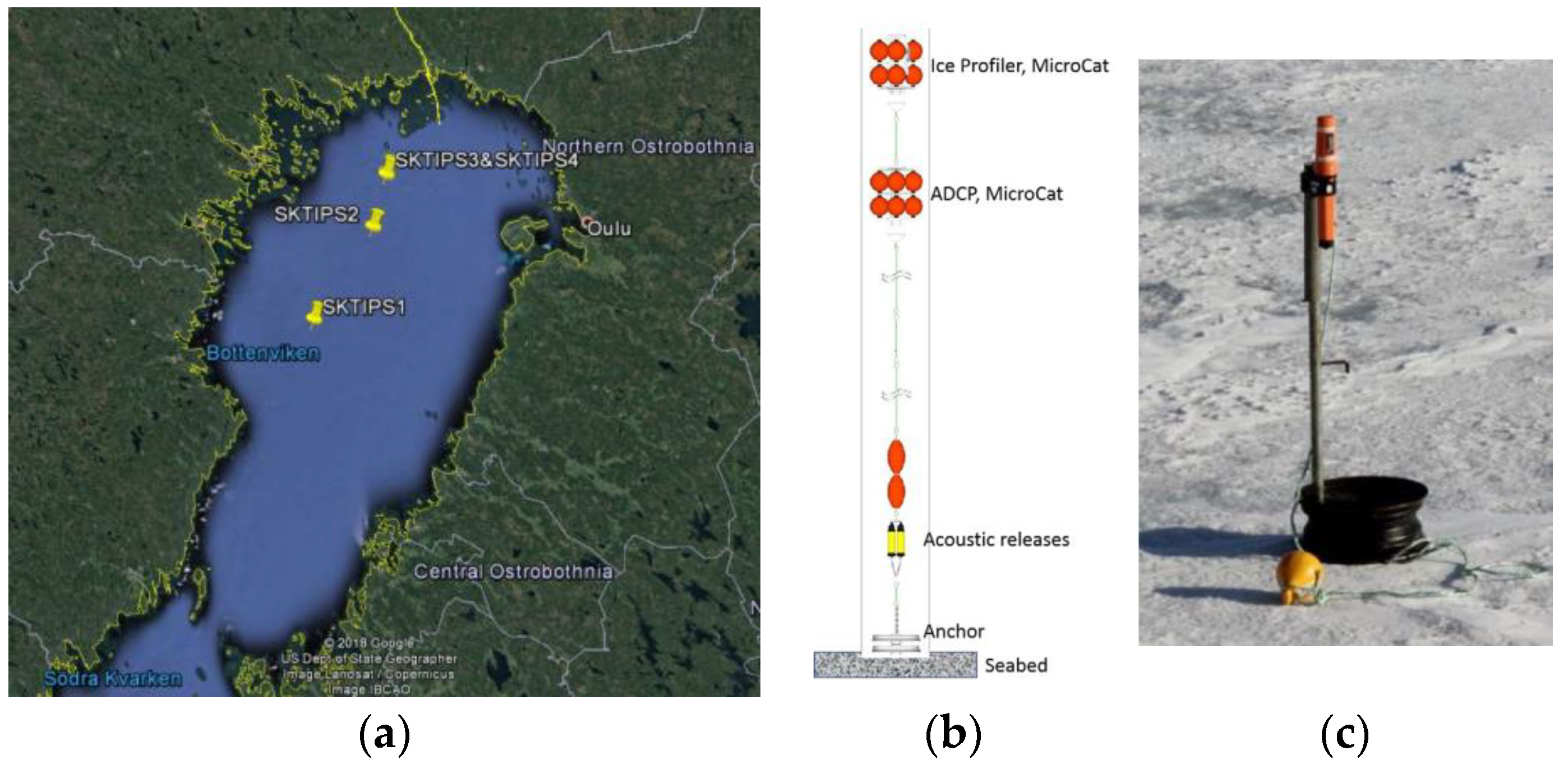
During the field experiment, various meteorological and oceanographic conditions such as air temperature, wind speed, wind direction, ice draft, ice drift speed, and ice concentration were recorded. Figure 23a illustrates the geographical positioning of the IPS stations in the Baltic Sea. Underwater ice profiler sensors (IPS) were strategically deployed and anchored to the seabed, as depicted in Figure 23b. For detailed information regarding the IPS stations, refer to Teigen, Lindvall, Samardzija, and Hansen [33]. These IPS stations were positioned approximately 35–35 m below the water surface to measure sea ice draft, as shown in Figure 23b. Acoustic Doppler Current Profilers (ADCPs) were utilized to measure ice drift speed and direction. Additionally, ice drift beacons were deployed on the surface of the ice to monitor ice drift velocity, as illustrated in Figure 23c.
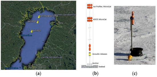
Figure 23.
(a) The spatial positions of the ice profilers within the Baltic Sea, (b) Stations for ice profiler sensors (IPS), and (c) Beacons for monitoring ice drift (DB) [34].
The station-keeping trials (SKTs) in the drifting ice project conducted a full-scale experiment using the icebreaker TV for ice management, aiming to break sea ice updrift from the stationary supply vessel to reduce ice loads. The experiment monitored ice drift locally using ADCP measurements and an ice drift beacon installed on the sea ice [33]. The ice rose diagram [34] illustrates the speed and direction of sea ice drift during these operations. Figure 24 shows the paths taken by the icebreaker and supply vessel for each operational pattern, delineated by latitude and longitude. Four different ice management schemes were implemented. The actual paths of the icebreaker differed slightly from planned routes due to variations in ice thickness, ice drift speed, and the vessel’s ice-breaking capabilities.
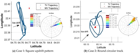
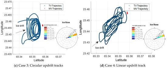
Figure 24.
Paths of the icebreaker TV and the supply vessel MV during station-keeping trials amidst drifting ice.
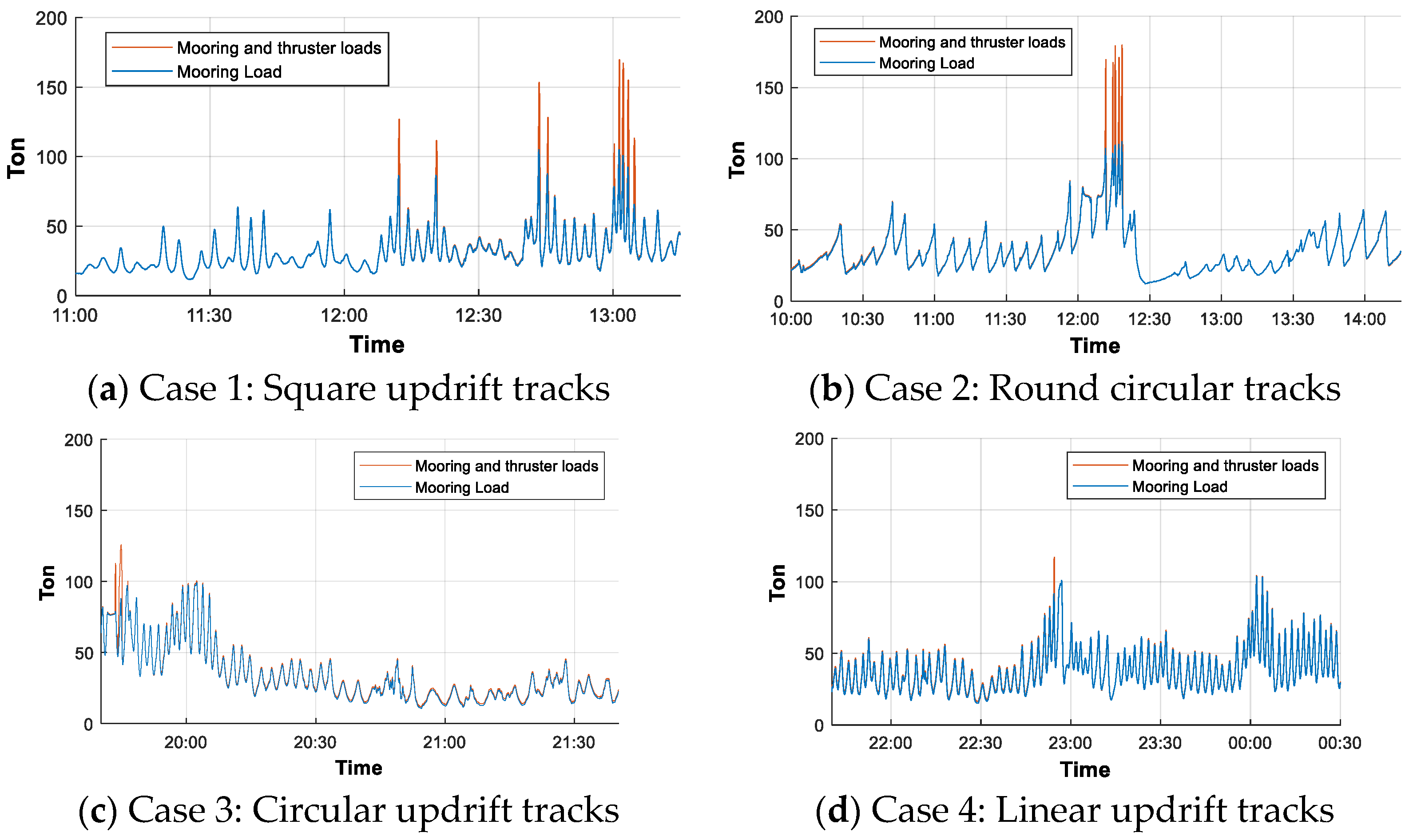
The mooring tension time series for each IM operation were captured using a load cell, recording data every second. Additionally, during instances where the mooring load exceeded 100 tons, the thrusters of the supply vessel MV were engaged for dynamic positioning-assisted mooring (DPAM), as depicted in Figure 25.
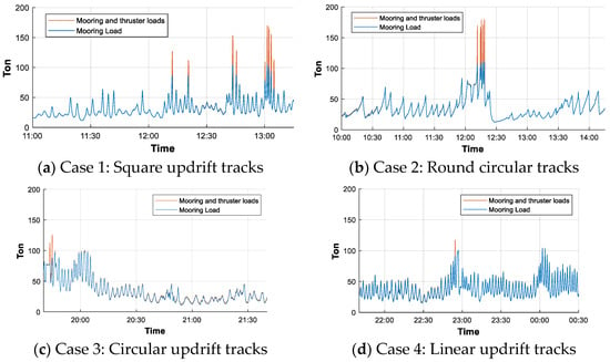
Figure 25.
The forces exerted by the mooring lines and active thrusters vary across different ice management strategies.
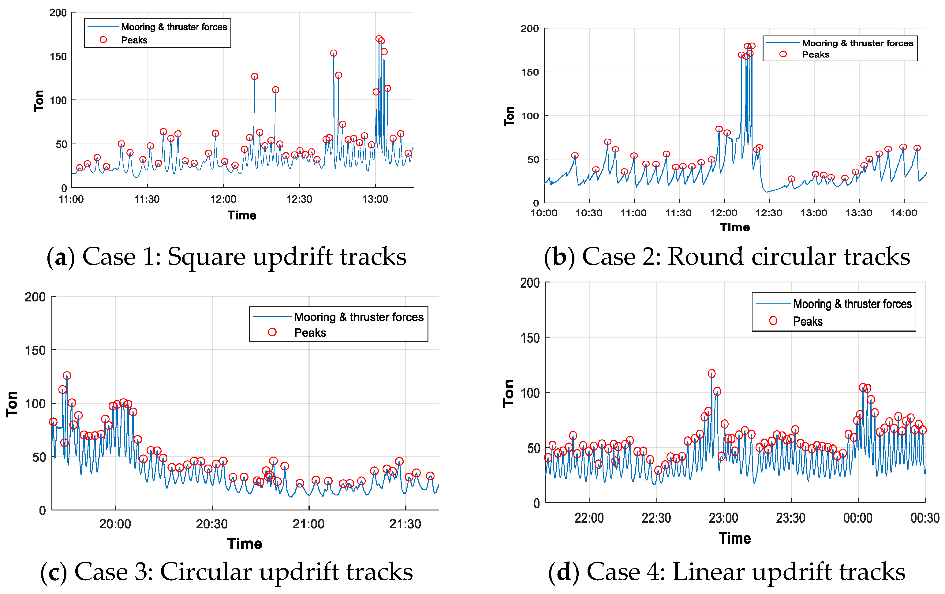
The peaks in the mooring line and thruster loads were calculated using the peaks prominence method to filter out local peaks caused by signal noise. A minimum prominence value of 2 tons was applied for peak detection in the analysis. The results of peak detection in the mooring load time series for various IM operation cases are shown in Figure 26.
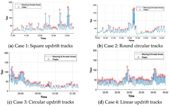
Figure 26.
Mooring and thruster forces for different ice management schemes.
The illustration in Figure 27 demonstrates the use of active thrusters to assist the mooring line when encountering an ice ridge. The load cell, which is the weakest component in the mooring line system, has a maximum capacity of approximately 150 tons. In this study, the analysis of short-term extreme mooring loads incorporates the total loads from both the mooring line and the thrusters.
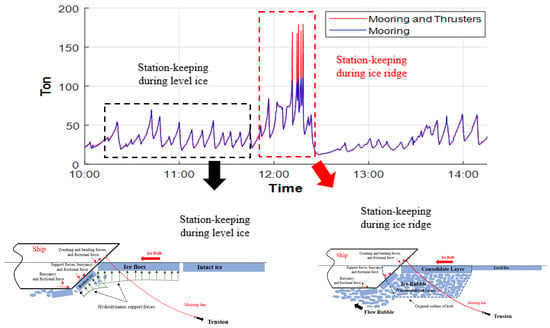
Figure 27.
The instance of active thrusters aiding the mooring line during Case 2: Circular round tracks.
4.2.4. Estimation of Global Ice Loading
The global ice loads on the vessel are computed using the ice resistance method, utilizing the time series data of ice thickness and ice drift speed. These loads are then compared with the recorded mooring loads observed during ice management operations. The ice resistance method, however, does not consider the impact of ice management, resulting in a systematic difference between the two datasets, as evident from the histograms in Figure 28. Additionally, findings from the SKT 2017 project by Fenz, Younan, Piercey, Barrett, Ralph, and Jordaan [35] indicate that well-organized ice management operations substantially reduce the local ice pressure on the ship’s bow during full-scale experiments. Table 2 compares the statistical parameters of the measured and calculated ice loads. It is important to note that the differences in the calculated loads across different cases are solely due to variations in ice thickness and drift speed, without accounting for differences in ice management schemes. The statistical variability of the calculated load is estimated based on the statistical properties of the input variables (i.e., ice thickness and drift speed).

Figure 28.
Histograms depicting the distribution of measured mooring loads compared to calculated (undisturbed) global ice loads for each ice management strategy.

Table 2.
The statistical parameters of the mooring loads for each IM scheme.
4.3. Extreme Value Estimation
In the context of ship and offshore structure design, extreme loading conditions play a critical role, especially in cold regions where sea ice loads dominate. Uncertainty in ice loading arises primarily from variations in sea ice properties during its formation [6]. The application of extreme value theory allows for the prediction of maximum ice loads on mooring lines by analyzing key parameters such as ice thickness and drift speed. Conversely, the extreme mooring loads can be directly estimated from measured peak loads in recorded time series data. This research focuses on deriving extreme mooring loads based on such peak measurements. For detailed data on ice conditions and metocean parameters during the SKT project, refer to Teigen, Lindvall, Samardzija, and Hansen [33].
4.3.1. The POT and PM Methods
The investigation focuses on assessing extreme mooring loads using peak values derived from the mooring load time series. This study contrasts the results obtained from employing two distinct methodologies: the POT approach and the BM method. In the context of the BM method, data points corresponding to peak values are subjected to fitting procedures involving various probabilistic models to identify an optimal parent distribution for subsequent extreme value analysis. Notably, the Gumbel distribution emerges as the most suitable model for characterizing extreme mooring load peaks under both the POT and BM methodologies. Illustrative instances of fitting mooring load peaks with the Gumbel distribution, particularly for scenarios involving the Square updrift pattern, are visually presented in Figure 29.

Figure 29.
Illustrates: (a) an instance of data fitting using the POT method, and (b) an instance of data fitting using the BM method for case 1: Square updrift pattern.
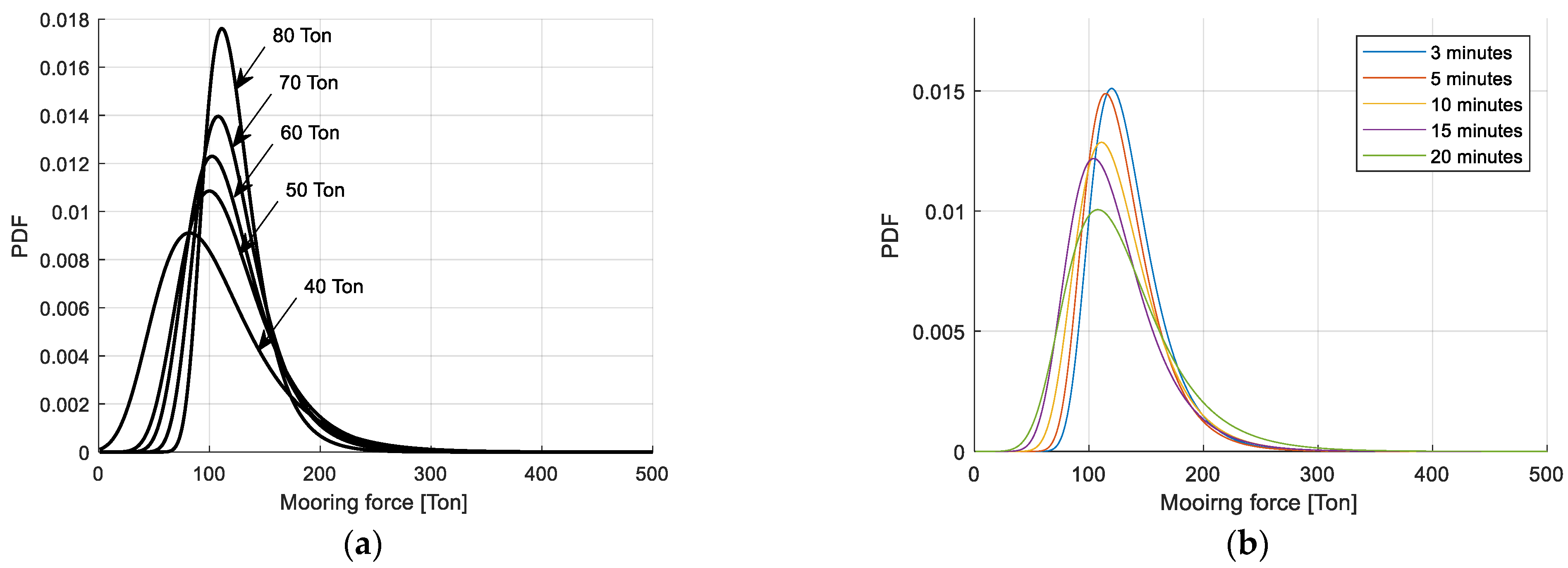
The analysis of extreme mooring load distributions derived from the POT and BM methods reveals their sensitivity to the chosen threshold value and the duration of the time window employed. Figure 30a depicts examples of PDFs representing extreme mooring loads for case 3, with variations in the threshold value. Careful deliberation is necessary when selecting the threshold value for the POT method, as higher thresholds diminish the dataset size available for statistical fitting purposes.
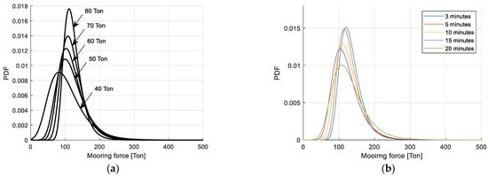
Figure 30.
(a) Examples of extreme mooring load PDFs for the circular updrift pattern with varying threshold values for the POT method, (b) examples of extreme mooring load PDFs with varying time window lengths for the BM method.
The temporal scope employed in the analysis of extreme mooring loads extends beyond that typically applied to assess the direct impacts of extreme ice loads on the ship hull, a timeframe usually ranging from 1 to 5 min [36,37]. This discrepancy arises because mooring load peaks result from the cumulative influence of all local ice loads acting on the ship hull. During station-keeping operations, when the ship initially encounters ice with minimal speed, the intervals between mooring load peaks are inherently longer compared to those between the peaks of local ice loads. In the present full-scale experimental setup, the duration of the time window used in the BM method ranges approximately from 3 to 20 min. Sensitivity analyses concerning the duration of this time window for the BM method, specifically for case 3 (the circular updrift pattern), are illustrated in Figure 30b.
The PDFs derived from the POT method generally yield higher values compared to the BM method for extreme peak loads, with the exception of case 3 (Suyuthi, Leira, and Riska [36]). Figure 31 illustrates a comparison of PDFs for extreme mooring loads obtained by the POT and BM methods across various ice management operation patterns.

Figure 31.
Comparison of extreme mooring load PDFs obtained by the POT and BM methods for each pattern of IM operation.
During the full-scale measurements, the mean values and standard deviations of the thickness of level ice, ice draft, and ice drift speed are documented as depicted in Figure 32a, Figure 32b, and Figure 32c, respectively. Statistical parameters for the level ice thickness and ice draft/ridges were computed based on the recorded IPS time series. However, the IPS records for ice draft do not differentiate between level ice thickness, consolidated layers, or ice rubble. Therefore, the maximum values of the past decade from drilling data concerning level ice thickness [38] in the Baltic Sea were utilized to distinguish between data pertaining to level ice thickness and ice draft/ridges in the time series.

Figure 32.
(a) The thickness of level ice during ice management activities. (b) The depth of the keel in the ice draft/ridge during ice management activities. (c) The speed of ice drift during ice management activities.
The highest-level ice thickness and ice draft occurred during IM operations for cases 3 and 4, respectively. Case 1, characterized by the square updrift pattern, experienced the highest ice drift speed, while the mean values of ice thickness and ice draft were lowest in this scenario.
The outcomes from the POT and BM methods regarding short-term extreme mooring loads reveal comparable patterns, demonstrating consistency in the results derived from these approaches. Both methods suggest an increased magnitude for the projected long-term extreme mooring loads across various return periods. This increase is adjusted using a reduction factor, R, specific to each ice management operation, as illustrated in Figure 33. The comparative analysis highlights that while the POT and BM methods generally align in their assessment of short-term extremes, there is a notable divergence in their long-term projections. The greatest disparity between the long-term extreme mooring loads estimated by the two methods is approximately 25 percent.

Figure 33.
Comparison of the extreme mooring forces estimated by various methods across different return periods, taking into account the impact of the reduction factor, R.
4.3.2. The ACER Method
The entire recorded time series for each Ice Management (IM) scheme was used to calculate ACER functions with k = 2, as detailed in Section 3.3.2. The resulting empirical ACER functions, for k = 2, were plotted against the amplitudes of mooring loads for each case in Figure 34. It is noteworthy that a Gumbel extreme value distribution would manifest as a straight line on these plots. Despite the limited quantity of available data, the plots of ACER functions suggest that the Gumbel distribution provides a reasonably accurate approximation of the extreme value distribution inherent in the data. This conclusion offers a robust foundation for its utilization in the BM method applied in this study, even with the constraints posed by limited data availability.
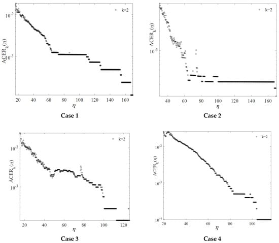
Figure 34.
Plot of barrier levels η versus ACER functions εk(η) for k = 2 on the logarithmic scale for different ice management schemes.
When the Gumbel distribution is considered an appropriate approximation for the extreme value distribution, the ACER and BM methods should, in theory, yield comparable results if properly implemented. However, in instances of limited data, significant uncertainty is associated with the estimates obtained from these various methods. Due to the BM method’s straightforward application and its confirmed applicability to our dataset, we have selected it as the reference method for this study.
5. Discussion
5.1. Probabilistic Assessment of Fixed Offshore Structures
Sea ice properties inherently exhibit significant uncertainty. The wide range between maximum and minimum parameter values used in calculating ice loading suggests that correlations between these parameters—whether high–high, high–low, or low–low—are likely to have a notable impact, a factor addressed in this study. It identified correlations among critical design parameters for both vertical and sloping structures. To integrate this understanding into our probabilistic assessment, it employs multivariate probability density functions with explicit correlation coefficients, alongside MCS techniques. This approach enables us to quantify how these correlations affect computed ice loads as per the ISO standard formulation. To ensure computational robustness, correlation coefficients range from −0.9 to 0.9, encompassing the full spectrum of possible values from strongly negative to strongly positive.
5.1.1. Vertical Structures
The level of uncertainty associated with ice loads is quantified using standard deviation, SD, where higher SD values indicate greater uncertainty. Additionally, the shapes of PDFs and CDFs provide insights into uncertainty levels; flatter PDFs and gentler CDF slopes suggest higher uncertainty.
5.1.2. Sloping Structures
In the case of sloping structures, parameters such as level ice thickness, rubble pile-up height, and flexural strength become crucial for estimating ice loading, particularly in scenarios involving thin ice, narrow structures, and no snow cover. This study utilized empirical formulas derived from data collected at the Kemi Lighthouse and Confederation Bridge to estimate the PDFs of accumulated rubble pile-up heights based on level ice thickness. Consequently, these conservative values from the Confederation Bridge data were adopted to compute global forces.
5.2. Extreme Value Analysis of Mooring Lines for Stationary Keeping in Ice
According to the offshore standard DNV-OS-H101 [39], for general marine operations, the design return period accepted depends on the reference period of field operations. For our current experiment, we focused on a one-week operation for the full-scale test, excluding installation, dynamic positioning tests, and others. The minimum accepted design return period for a one-week operation is three months, utilized specifically for short-term extreme value analysis. However, it is important to note that this offshore standard was initially designed for operations conducted in open water.
For a three-month return period, considering a reduction factor R corresponding to an operation frequency of 0.375, case 4 (representing the linear updrift scheme) resulted in the highest extreme mooring forces: 320 tons for POT, 318 tons for ACER, and 298 tons for BM. These values exceed both the load cell capacity (150 tons) and the minimum breaking load (MBL = 223 tons) of the steel wire. Conversely, the lowest extreme mooring load occurred in case 3, the circular updrift pattern, yielding estimates of 227 tons for POT, 225 tons for ACER, and 274 tons for BM. To align with the load cell capacity and the steel wire’s minimum breaking load, reduction factors R of approximately 0.0025 and 0.05 are necessary, respectively.
Notably, during case 2, the recorded maximum ice load exceeded 150 tons when an ice ridge passed the supply vessel, as depicted in Figure 28’s time series data. During this period, mooring relied on the vessel’s thrusters. This underscores the inadequacy of the current low value of the operational reduction factor R, particularly for scenarios lacking thruster assistance.
The findings reveal that the highest efficiency of IM operations when considering average unit ice momentum occurs in case 3: the circular updrift pattern. This observation aligns with the relative efficiency determined by considering only the ice thickness/draft. However, the efficiency for case 1, the square updrift pattern, increases when momentum is taken into account due to the highest ice drift speed in this scenario, which elevates the average sea ice momentum. Conversely, the lowest efficiency for the momentum criterion is observed in case 2, which slightly diverges from the results obtained by solely considering the ice thickness/draft.
In case 2, where the icebreaker follows a round circular pattern, it covers the entire vicinity around the supply vessel, MV. As a result, the effectiveness of icebreaking in the upstream direction of the ice drift decreases due to the shorter distance over which the sea ice is cut. This reduction in travel distance tends to lower the efficiency of the ice management operation. However, the round circular pattern offers advantages in regions characterized by rapidly changing directions of ice drift.
The short-term extreme mooring loads estimated by the POT, ACER, and BM methods for each IM scheme are normalized based on the maximum observed mooring load, as shown in Figure 35. The highest normalized values were observed for case 4, the linear updrift pattern, resulting in 3.1, 3.0, and 2.8 for the POT, ACER, and BM methods, respectively. Typically, the maximum loads derived from simulations of severe environmental conditions are used for mooring system designs. The normalization results suggest a notable increase in long-term extreme values compared to maximum loads observed during short-term operations.
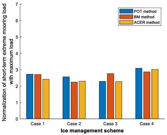
Figure 35.
Normalization of Extreme Loading by maximum observed force during the tests [40].
Typically, there are several international standards for mooring design, such as DNVGL (DNVGL, 2015), GL Noble Denton (Denton, 2013), American Bureau of Shipping (ABS) (ABS, 2018), Bureau Veritas (Veritas, 2005), etc. The safety factors in the international design standards are introduced in order to cover the uncertainty related to the estimated extreme loads and structural resistance.
Usually, there exist multiple global standards governing mooring design, such as DNVGL [41], American Bureau of Shipping (ABS) [42], GL Noble Denton [43], Bureau Veritas [44], etc. The safety margins prescribed by international design standards serve to mitigate uncertainties linked to estimated extreme loads and structural resilience.
Moreover, the mooring system includes a weak link at the load cell and a safety wire intended to disengage in uncontrollable scenarios, thus bolstering operational safety. It is noteworthy that extreme value analysis is pivotal in mooring system design for forecasting the maximum expected loading conditions during operations.
This study quantifies safety factors in terms of reserve strength capacity, defined as the ratio between the minimum breaking load (MBL = 611 tons) of the main mooring chain (76 mm type R4) and the maximum extreme mooring load. The mooring line exhibits a reserve strength of approximately 1.9 (MBL/maximum extreme mooring load = 611 tons). It is observed that the reserve strength capacity of the main mooring chain falls slightly below the safety factors stipulated by key design standards such as DNVGL (safety factor = 1.9), ABS (safety factor = 2.25), GL Noble Denton (safety factor = 1.67), and Bureau Veritas (safety factor = 1.67). For longer return periods (e.g., 1 year), this suggests the necessity for stronger mooring lines.
6. Conclusions
A probabilistic evaluation of ice-structure interaction loads, employing MCS methods, was undertaken based on the ISO standard formula. The study encompassed two structural configurations: vertical and sloping. Correlation coefficients between the ice strength coefficient and ice thickness, and between flexural strength and ice thickness, were estimated to assess their impact on uncertainties associated with ice loads across varying correlation coefficient values.
The analysis demonstrated that increasing correlation coefficients substantially heightened both global ice forces and associated uncertainties compared to scenarios with zero correlation:
- For vertical structures, a transition from a correlation coefficient of 0 to 0.9 resulted in approximately 10% and 40% increases in mean values and standard deviations.
- Sloping structures showed approximately 20% and 60% increases in mean value and standard deviation of horizontal and vertical global forces, respectively, as correlation coefficients increased from 0 to 0.9.
- Higher sloping angles correlated with an increased standard deviation (uncertainty) of global forces.
- Changes in slope angle exerted a more pronounced effect on mean values and standard deviations of global forces in the horizontal direction compared to the vertical direction.
Short-term analysis of extreme mooring loads from full-scale measurements under various ice management strategies was undertaken. These strategies encompass square updrift, round circle, circular updrift, and linear updrift patterns. The experiment monitored mooring line tension via a load cell, with continuous recording of measurements. The analysis focuses on peaks in the mooring load time series using POT and BM methods to ascertain the statistical properties of short-term extreme mooring loads.
- The results are notably sensitive to the POT threshold and the time window width applied in the BM method.
- Extreme mooring loads estimated for a three-month return period, adjusted with a reduction factor R for an operational frequency of 0.375, exhibit consistent agreement across all methods.
- Differences among results from the various methods do not exceed 20%, primarily influenced by variability in peak mooring loads (also correlating with total ice loads on the MV supply vessel).
- Case 3, employing the circular updrift pattern, demonstrates the highest efficiency among the ice management schemes, followed by case 4 utilizing the linear updrift pattern. Case 2, employing the round circular pattern, displays the lowest efficiency.
In conclusion, rigorous analysis of extreme mooring loads is essential for designing mooring systems to ensure adequate safety and operational integrity, particularly for temporary operations in Arctic environments.
As for future work, it is suggested that more effort should be assigned to the data from full-scale measurements to enhance the accuracy of the probabilistic models. This is important to ensure that sufficient safety and integrity levels of these structures can be maintained throughout the lifetime of their operation. More attention should also be paid to the uncertainty of ice load estimation.
Author Contributions
Conceptualization, C.S., B.J.L. and K.V.H.; methodology, C.S., W.C., A.N. and S.K.; software, C.S., A.N. and W.C.; validation, C.S. and W.C.; formal analysis, C.S.; investigation, C.S., B.J.L. and K.V.H.; resources, K.V.H.; data curation, C.S. and W.C.; writing-original draft preparation, C.S., B.J.L. and W.C.; writing-review and editing, C.S., B.J.L. and W.C.; visualization, S.K., C.C., I.S. and S.X.; supervision, B.J.L., K.V.H., A.N. and S.K.; project administration, B.J.L., K.V.H. and S.K.; funding acquisition, B.J.L., K.V.H. and S.K. All authors have read and agreed to the published version of the manuscript.
Funding
This work is supported by the NTNU Oceans Pilot Project Risk, Reliability and Ice Data in Arctic Marine Environments. This research is partially supported by the NSRF through the Program Management Unit for Human Resources & Institutional Development, Research, and Innovation [grant number B39G660028]. This work is supported by the Department of Civil Engineering, Faculty of Engineering, Chiang Mai University. This research was partially supported by Chiang Mai University.
Institutional Review Board Statement
Not applicable.
Informed Consent Statement
Not applicable.
Data Availability Statement
Data are contained within the article.
Conflicts of Interest
The authors declare no conflict of interest.
References
- Pfaffling, A.; Haas, C.; Reid, J.E. Direct helicopter EM—Sea-ice thickness inversion assessed with synthetic and field data. Geophysics 2007, 72, F127–F137. [Google Scholar] [CrossRef]
- Li, H.; Bjerkås, M.; Høyland, K.V.; Nord, T. Panel loads and weather conditions at Norströmsgrund lighthouse. In Proceedings of the 23rd IAHR International Symposium on Ice, Ann Arbor, MI, USA, 31 May–3 June 2016. [Google Scholar]
- Zvyagin, P. A method for the probabilistic modelling of ice pressure. Cold Reg. Sci. Technol. 2015, 118, 112–119. [Google Scholar] [CrossRef]
- ISO19906:2010; Petroleum and Natural Gas Industries–Arctic Offshore Structures. ISO: Geneva, Switzerland, 2010.
- Ranta, J.; Polojärvi, A.; Tuhkuri, J. Ice loads on inclined marine structures-Virtual experiments on ice failure process evolution. Mar. Struct. 2018, 57, 72–86. [Google Scholar] [CrossRef]
- Sinsabvarodom, C.; Chai, W.; Leira, B.J.; Høyland, K.V.; Naess, A. Uncertainty assessments of structural loading due to first year ice based on the ISO standard by using Monte-Carlo simulation. Ocean Eng. 2020, 198, 106935. [Google Scholar] [CrossRef]
- Lemström, I.; Polojärvi, A.; Puolakka, O.; Tuhkuri, J. Load distributions in the ice-structure interaction process in shallow water. Ocean Eng. 2022, 258, 111730. [Google Scholar] [CrossRef]
- Hamilton, J.; Holub, C.; Blunt, J.; Mitchell, D.; Kokkinis, T. Ice management for support of arctic floating operations. In Proceedings of the OTC Arctic Technology Conference, Houston, TX, USA, 5–7 November 2018. [Google Scholar]
- Gürtner, A.; Baardson, B.H.H.; Kaasa, G.-O.; Lundin, E. Aspects of importance related to Arctic DP operations. In Proceedings of the International Conference on Offshore Mechanics and Arctic Engineering, Rio de Janeiro, Brazil, 1–6 July 2012; American Society of Mechanical Engineers: New York, NY, USA, 2012; pp. 617–623. [Google Scholar]
- American Petroleum Institute. Recommended Practice for Design and Analysis of Stationkeeping Systems for Floating Structures; American Petroleum Institute: Washington, DC, USA, 1996. [Google Scholar]
- Liferov, P.; McKeever, T.; Scibilia, F.; Teigen, S.H.; Kjøl, A.; Almkvist, E.; Lindvall, J.K. Station-keeping trials in ice: Project overview. In Proceedings of the ASME 2018 37th International Conference on Ocean, Offshore and Arctic Engineering, Madrid, Spain, 17–22 June 2018; American Society of Mechanical Engineers: New York, NY, USA, 2018; p. V008T007A029. [Google Scholar]
- Croasdale, K.R.; Cammaert, A.B. An improved method for the calculation of ice loads on sloping structures in first-year ice. Hydrotech. Constr. 1994, 28, 174–179. [Google Scholar] [CrossRef]
- Brown, T.G.; Määttänen, M. Comparison of Kemi-I and Confederation Bridge cone ice load measurement results. Cold Reg. Sci. Technol. 2009, 55, 3–13. [Google Scholar] [CrossRef]
- Riska, K. Performance of Merchant Vessels in Ice in the Baltic; Sjöfartsverket: Norrkoping, Sweden, 1997. [Google Scholar]
- Erceg, S.; Ehlers, S. Semi-empirical level ice resistance prediction methods. Ship Technol. Res. 2017, 64, 1–14. [Google Scholar] [CrossRef]
- Sinsabvarodom, C.; Leira, B.J.; Høyland, K.V.; Næss, A.; Chai, W. A generalized ice drift spectrum based on measurements in the Beaufort Sea. Ocean Eng. 2024, 296, 116832. [Google Scholar] [CrossRef]
- Riska, K. Design of Ice Breaking Ships. 2011. Available online: https://www.eolss.net/sample-chapters/C05/E6-178-45-00.pdf (accessed on 24 July 2024).
- Kämäräinen, J. Evaluation of Ship Ice Resistance Calculation Methods. Licentiate Thesis, Helsinki University of Technology, Otaniemi, Finland, 1993. [Google Scholar]
- Ionov, B. Ice Resistance and Its Composition; Arctic and Antarctic Research Institute: Saint Petersburg, Russia, 1988. [Google Scholar]
- Lindquist, A. Straightforward method for calculation of ice resistance of ships. In Proceedings of the 10th International Conference, Port and Ocean Engineering under Arctic Conditions, POAC’89, Luleaa, Sweden, 12–16 June 1989. [Google Scholar]
- Mellor, M. Ship resistance in thick brash ice. Cold Reg. Sci. Technol. 1980, 3, 305–321. [Google Scholar] [CrossRef]
- Kuuliala, L.; Kujala, P.; Suominen, M.; Montewka, J. Estimating operability of ships in ridged ice fields. Cold Reg. Sci. Technol. 2017, 135, 51–61. [Google Scholar] [CrossRef]
- Hopkins, M.A.; Hibler, W., III; Flato, G. On the numerical simulation of the sea ice ridging process. J. Geophys. Res. J. Geophys. Res. Ocean. 1991, 96, 4809–4820. [Google Scholar] [CrossRef]
- Liu, P.-L.; Der Kiureghian, A. Multivariate distribution models with prescribed marginals and covariances. Probabilistic Eng. Mech. 1986, 1, 105–112. [Google Scholar] [CrossRef]
- Goda, Y. On the methodology of selecting design wave height. Coast. Eng. 1989, 1988, 899–913. [Google Scholar]
- Far, S.S.; Wahab, A.K.A. Evaluation of peaks-over-threshold method. Ocean Sci. Discuss. 2016, 2016, 1–25. [Google Scholar]
- Næss, A.; Gaidai, O. Estimation of extreme values from sampled time series. Struct. Saf. 2009, 31, 325–334. [Google Scholar] [CrossRef]
- Naess, A.; Gaidai, O.; Karpa, O. Estimation of extreme values by the average conditional exceedance rate method. J. Probab. Stat. 2013, 2013, 797014. [Google Scholar] [CrossRef]
- El Bakkay, B.; Coche, E.; Riska, K. Efficiency of Ice Management for Arctic Offshore Operations. Int. Conf. Offshore Mech. Arct. Eng. 2014, 45561, V010T007A041. [Google Scholar] [CrossRef]
- Kjøl, A.; Liferov, P.; Almkvist, E.; Lindvall, J.K.; McKeever, T. Station-keeping trials in ice: Marine spread. In Proceedings of the International Conference on Offshore Mechanics and Arctic Engineering, Madrid, Spain, 17–22 June 2018; American Society of Mechanical Engineers: New York, NY, USA, 2018; p. V008T007A023. [Google Scholar]
- Neville, M.; Almkvist, E.; Scibilia, F.; Lindvall, J.K.; Liferov, P. Station-keeping trials in ice: Overview of ice management support. In Proceedings of the ASME 2018 37th International Conference on Ocean, Offshore and Arctic Engineering, Madrid, Spain, 17–22 June 2018; American Society of Mechanical Engineers: New York, NY, USA, 2018; p. V008T007A027. [Google Scholar]
- Sinsabvarodom, C.; Leira, B.J.; Chai, W.; Naess, A. Extreme Value Estimation of Mooring Loads Based on Station-Keeping Trials in Ice. In Proceedings of the ASME 2020 39th International Conference on Ocean, Offshore and Arctic Engineering, Online, 3–7 August 2020; American Society of Mechanical Engineers: New York, NY, USA, 2020. [Google Scholar]
- Teigen, S.H.; Lindvall, J.K.; Samardzija, I.; Hansen, R.I. Station-keeping trials in ice: Ice and metocean conditions. In Proceedings of the ASME 2018 37th International Conference on Ocean, Offshore and Arctic Engineering, Madrid, Spain, 17–22 June 2018; American Society of Mechanical Engineers: New York, NY, USA, 2018; p. V008T007A030. [Google Scholar]
- Sinsabvarodom, C.; Chai, W.; Leira, B.J.; Høyland, K.V.; Naess, A. Probabilistic Assessment of Ice Rose Diagrams for Ice Drift in the Beaufort Sea. In Proceedings of the 25th International Conference on Port and Ocean Engineering under Arctic Conditions, Delft, The Netherlands, 9–13 June 2019. [Google Scholar]
- Fenz, D.; Younan, A.; Piercey, G.; Barrett, J.; Ralph, F.; Jordaan, I. Field measurement of the reduction in local pressure from ice management. Cold Reg. Sci. Technol. 2018, 156, 75–87. [Google Scholar] [CrossRef]
- Suyuthi, A.; Leira, B.J.; Riska, K. Non Parametric Probabilistic Approach of Ice Load Peaks on Ship Hulls. In Proceedings of the ASME 2012 31st International Conference on Ocean, Offshore and Arctic Engineering, Rio de Janeiro, Brazil, 1–6 July 2012; pp. 415–423. [Google Scholar]
- Chai, W.; Leira, B.J.; Naess, A. Probabilistic methods for estimation of the extreme value statistics of ship ice loads. Cold Reg. Sci. Technol. 2018, 146, 87–97. [Google Scholar] [CrossRef]
- Ronkainen, I.; Lehtiranta, J.; Lensu, M.; Rinne, E.; Haapala, J.; Haas, C. Interannual sea ice thickness variability in the Bay of Bothnia. Cryosphere 2018, 12, 3459–3476. [Google Scholar] [CrossRef]
- DNV-OS-H101; Marine Operations, General. October 2011. Available online: https://rules.dnv.com/docs/pdf/dnvpm/codes/docs/2011-10/Os-H101.pdf (accessed on 2 July 2024).
- Sinsabvarodom, C.; Leira, B.J.; Chai, W.; Næss, A. Short-term extreme mooring loads prediction and fatigue damage evaluation for station-keeping trials in ice. Ocean Eng. 2021, 242, 109930. [Google Scholar] [CrossRef]
- DNVGL-OS-E301; Position Mooring. DNV GL: Oslo, Norway, 2015.
- ABS. Guide for Position Mooring Systems; American Bureau of Shipping Incorporated by Act of Legislature of the State of New York: New York, NY, USA, 2018.
- GL Noble Denton. Technical Policy Board Guidelines for Moorings, GL Noble Denton 0032/ND; GL Noble Denton: Loughborough, UK, 2013. [Google Scholar]
- NR493; Classification of Mooring Systems for Permanent and Mobile Offshore Units. Bureau Veritas Marine & Offshore: Paris, France, 2005.
Disclaimer/Publisher’s Note: The statements, opinions and data contained in all publications are solely those of the individual author(s) and contributor(s) and not of MDPI and/or the editor(s). MDPI and/or the editor(s) disclaim responsibility for any injury to people or property resulting from any ideas, methods, instructions or products referred to in the content. |
© 2024 by the authors. Licensee MDPI, Basel, Switzerland. This article is an open access article distributed under the terms and conditions of the Creative Commons Attribution (CC BY) license (https://creativecommons.org/licenses/by/4.0/).

