Abstract
The global transition to renewables in response to climate change has largely been supported by the expansion of wind power capacity and improvements in turbine technology. This is being made possible mainly due to improvements in the design of highly efficient turbines exceeding a 10 MW rated power. Apart from power efficiency, wind turbines must withstand the mechanical stress caused by wind–hydro conditions. Such comprehensive structural analysis has rarely been performed previously, especially for large-scale wind turbines under real environmental conditions. The present work analyzes the energy production and structural performance of an NREL-IEA 15 MW wind turbine using measured wind and hydro data. First of all, an optimum operating range is determined in terms of the wind speed and blade pitch angle to maximize the power coefficient. Then, at this optimum range, a detailed breakdown of the forces and moments acting on different components of the wind turbine is presented. It was found that wind speeds of 9 to 12 m/s are best suited for this wind turbine, as the power coefficient is at its maximum and the mechanical loads on all components are at a minimum. The loads are at a minimum due to the optimized blade pitch angle. The bending force on a monopile foundation (fixed on the seabed) is found to be at a maximum and corresponds to nearly 2000 kN. The maximum blade force is nearly 700 kN, whereas on the tower it is almost 250 kN. The maximum force on the tower occurs at a point which is found to be undersea, whereas above-sea, the maximum force on the tower is nearly 20% less than the undersea maximum force. Finally, seasonal and annual energy production is also estimated using locally measured wind conditions.
1. Introduction
Fixed offshore wind farms are a promising breakthrough technology for wind energy harvesting due to their ability to produce power at nearshore depths between 25 and 40 m, resulting in a large capacity [1,2]. The most common fixed-type offshore foundation is a monopile foundation [1]. A report by the Commission of the European Union [2] emphasizes the importance of utilizing fixed offshore energy to achieve renewable energy targets. Installing floating turbines in deep oceans away from the coast offers various challenges, including increased water depth and high wave turbulence intensity [3]. In energy systems with a high green energy penetration, these components are crucial to wind turbine installation costs.
Bento and Fontes [3] identified high costs and underdeveloped technology as major impediments to floating wind development. According to sources within the industry, floating wind turbines are more expensive per operational kW than fixed-bottom wind turbines or land-based wind turbines [4]. Experts estimate a reduction of forty percent in median costs by 2050 [5]. The panel noted that cost reductions were primarily driven by advancements in monopile foundation design and manufacture, transportation and installation, and efficiencies of scale. In fixed-bottom offshore and wind farm projects, increased turbine capacity is the primary savings factor. Fixed wind power may benefit from economies of scale, as demonstrated by a past study [5]. Larger and taller rotors not only increase gross load factors, but also have a significant impact on the floating platform and installation costs per kW. Offshore operations allow for the installation of huge machines without constraints on transportation. Manufacturers are designing blades in the 12–15 MW output range, and existing blades are becoming larger [3,6]. The process of “upscaling” involves increasing size to reduce the Levelized Cost of Energy (LCOE). Upscaling offers an opportunity to reduce the LCOE, especially in offshore operations where turbine sizes are typically bigger [4]. According to references [3,5], the learning rates for floating offshore projects range between 15 and 20%. Kikuchi and Ishihara [7] discovered that utilizing a design model to scale up a 2 MW floating offshore wind turbine to 10 MW can lower capital expenses per kilowatt by as much as 57%. Longer blades that cross the boundary layer of the atmosphere in the top portion of each revolution may impact preventative care methods for offshore uses, according to the latest research [8,9]. An increasing blade size is going to have an impact on deployment. Jiang et al. [10] found that fixed-bottom turbines may experience worsened blade assembly issues. It is important to note that FOWTs are frequently set up in harbors [11] before they are taken to the deployment location. Improving infrastructure and procedures to handle larger wind turbines is currently one of the most important issues.
Literature Survey
To develop novel rotor designs, an upscaling technique is typically used as a starting point for improvement. For example, the DTU10 MW Reference Wind Turbine (RWT) [12] has become widely used. An increased rotor size presents known problems, including increased mass and load [13]. Technological developments in rotor design can minimize the LCOE by embracing modern design trends like a high swept area and low area-specific power. Ashuri [14] found a less-than-square trend between rotor power and diameter. In FOWTs, expanding can be used to create support platforms for larger wind turbines. Leimeister et al. [15] address the issues of scaling FOWT semi-submersible-type floaters. Ferri et al. [16] suggested an optimization approach that can minimize the peak response amplitude operator (RAO) in pitch by up to 50% compared to typical scaling based on the turbine power ratio square root. Kikuchi and Ishihara [7] compared two upscaling strategies for FOWT platforms and proposed a third. The authors found that using the recommended methodologies results in a support structure that can withstand overturning thrust pressures while significantly lowering the per kW costs.
FOWTs have more complicated loading patterns than stationary or onshore wind turbines. Mounting a turbine on a floating base may result in increased gravitational and inertial forces [17]. In a Horizontal Axis Wind Turbine (HAWT), the rotor and hub mass are elevated above the level of the ocean. The turbine’s “inverted pendulum” behavior creates additional loading on its components, particularly the tower [18]. This impact is widely known. According to Jonkman and Matha [19], installing turbine components on a spar-type or barge-type floating platform increases both the ultimate and fatigue loads. The impact is also observed on semi-submersible platforms, as reported in [20]. Increases in weight, rotary covered area, and tower height can cause significant weights and instability moments [21], posing a serious problem in terms of load escalation.
The NREL-IEA fifteen megawatt has been utilized as a case study in the present work [22,23]. Researchers have examined many floater theories over time [24]. Barge-type layouts can cause significant sea-to-land stress multiplication on turbines [18,24]. However, alternative floater types, such as spar floaters, tension-leg systems, and semi-submersibles, possess distinct benefits. Monopile foundations are gaining popularity due to their ease of transport, short draft, and durability in wind and wave situations [25].
There are numerous studies which focus on either the field testing or experiment-based performance evaluation of large-scale horizontal axis wind turbines (HAWTs). For example, the Model Rotor Experiment in Controlled Conditions (MEXICO) and the Unsteady Aerodynamics Experiment (UAE) constitute two of the most important HAWT investigations. NREL completed the UAE in stages. While Stages I–IV were field investigations from 1989 to 1997 [26,27], Stage VI was a wind tunnel test conducted in 2000. A two-bladed rotor with a diameter of ten meters was carefully equipped and deployed in the NASA Ames wind tunnel for testing [28]. The MEXICO trial was carried out in 2006 at the German–Dutch Wind Tunnel (DNW). Detailed aerodynamics measurements, including pressure, loads, and three-dimensional flow field characteristics, were collected using particle image velocimetry (PIV) on a three-bladed rotor with a diameter of 4.5 m [29,30]. The follow-up initiative called “New Mexico” was launched in 2014 to collect new data [31]. The findings from these two experimental campaigns were thoroughly examined and utilized to validate and calibrate simulation tools with varied fidelity levels. Schepers and Schreck [32] provide a detailed assessment of the literature relating to these two research studies. Following the success of the preceding two experiments, the present databases were enlarged by conducting additional tests on scaled copies of the two rotors. Xiao et al. [33] investigated the wake of a 1:8 sized replica of the UAE Phase VI rotor using the PIV. Cho and Kim [34] from the Korean Aerospace Research Institute (KARI) investigated the influence of the Reynolds number on both power and torque using a 1:5 size replica of the UAE Phase VI turbine. The same team conducted comparable studies on a smaller-scale version of the MEXICO rotor (2:4.5) [35]. The Spanish National Institute for Aerospace Technology (INTA) developed a 1:4 size MEXICO rotor. Schepers et al. [36] compared the scaled model results with the original MEXICO data from IEA Project 29.
In addition to laboratory experiments, HAWTs are comprehensively studied utilizing computational models. Several reference wind turbine (RWT) prototypes have been built over the last decade to allow comparisons between different simulation programs and to promote collaboration between academic and industrial investigations, including the National Renewable Energy Laboratory five megawatt RWT [22], the Denmark Technical University ten megawatt RWT [12], and the International Energy Agency’s fifteen megawatts RWT [23]. While such freely available reference models do not include operational wind turbines, they accurately reflect current HAWT technological advances and improvements. Wind tunnel tests were conducted using scaled prototypes of these benchmark wind turbines to obtain experimental results that may be utilized to validate numerical calculations. Berger et al. [37] created a prototype turbine modeled on the NREL five megawatt RWT, which has since been utilized to investigate dynamic inflow issues related to pitch changes [38] and interactions between fluids and structures using photography [39,40]. Fontanella et al. [41] conducted experiments on a downsized DTU ten-megawatt wind turbine that simulated the movements of a floating offshore wind turbine (FOWT). Along with the load cell data on the wind turbine, the wake was described by PIV data. Taruffi et al. [42] also conducted similar tests, increasing the imitated floater motions to six degrees of freedom with greater amplitudes and frequency. Fontanella et al. [43] carried out more trials on a one hundred sized prototype of the IEA 15 MW RWT produced by Allen et al. [44]. Rotor loads were captured with load cells, and the aftermath was described with hot-wire acceleration observations. Kimball et al. [45] investigated a 1:70 sized prototype of the IEA fifteen megawatt, with a focus on verifying the force and torque profiles and confirming the pitch actuator. While these investigations on smaller versions of RWTs provide useful information about rotor-level aerodynamics, they require more detailed knowledge about blade dynamics.
Discreet measurement methods like laser Doppler velocimetry (LDV) and stereoscopic particle image velocimetry (SPIV) can be used to gather such blade-level information. Phengpom et al. [46,47,48] used LDV to investigate the flow field near the blade. Akay et al. [49] investigated the vortex structure surrounding the blade’s base of a two-bladed wind turbine having a diameter of two meters using SPIV observations. Similarly, Lignarolo et al. [50] investigated the wake evolution of a smaller model (two blades, 0.6 m diameter), focusing on tip vortices. Micallef et al. [51,52] expanded on this line of research by studying the production of the tip vortex in greater detail on a separate two-bladed wind turbine replica of two meters in diameter. In addition, and most pertinent to the current work, del Campo et al. [53,54] employed SPIV to calculate the longitudinally blade distribution of loads in an HAWT for radial and yawed inflow.
The present study analyzes the performance of the NREL-IEA 15 MW wind turbine on a monopile foundation, i.e., installed in shallow waters and with a foundation fixed on the seabed, utilizing measured wind and wave data. The current literature lacks such work in which the energy and structural performance of large-scale wind turbines are investigated together in detail using measured wind and wave data. This work aims to fulfil that gap in the literature which will help to design optimum wind farms using large-scale wind turbines such as the NREL-IEA 15 MW. The methodology and results presented in the current work can be unanimously adopted for any other local geographical, hydro, wind, and/or environmental conditions. The flowchart shown in Figure 1 briefly explains the main contents of the present paper.
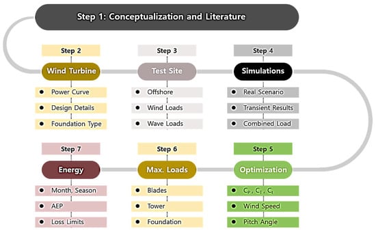
Figure 1.
Technical schematics and main contents of the present study.
2. Materials and Methods
2.1. Wind Turbine Model
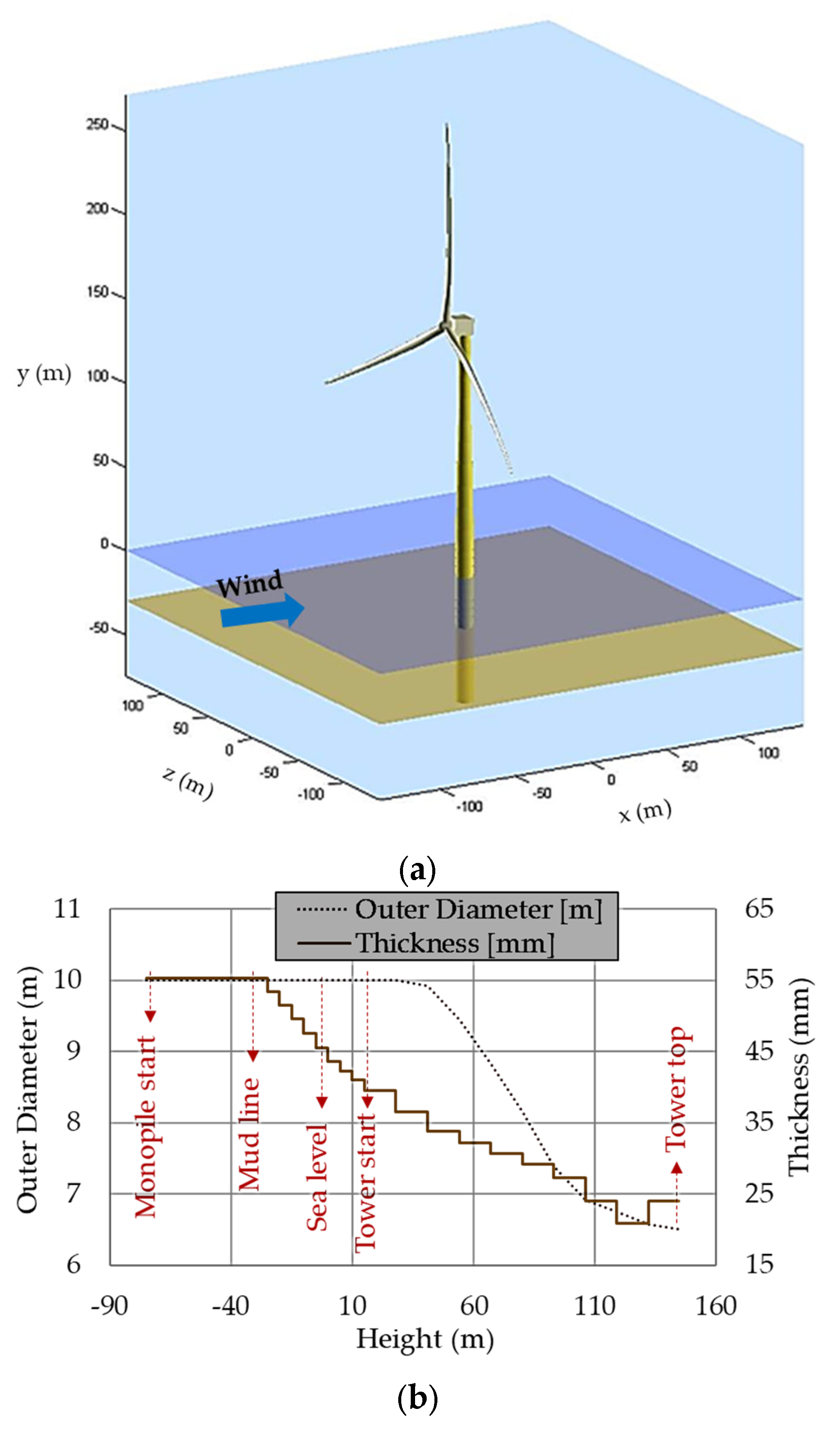
The wind turbine model selected for extreme analysis is the NREL-IEA 15 MW. There are a few reasons for selecting this wind turbine model. One is that, as explained above, large-size wind turbines are more energy-efficient and have a relatively higher power coefficient. The second reason is that almost all of the features and characteristics of this wind turbine model are publicly available. The latter mentioned reason is very crucial as the present study requires such detailed information for comprehensive load and energy analysis. The prominent design features and properties of this wind turbine model are mentioned in Figure 2.
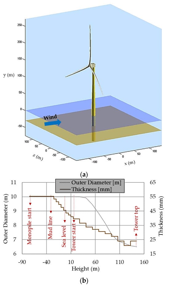
Figure 2.
NREL-IEA 15 MW wind turbine: (a) BLADED model; (b) monopile and tower dimensions.
In the present study, the wind turbine model has been analyzed in commercial software named BLADED. Figure 2 shows the geometry and dimensions of the modeled wind turbine. The dimensions are exactly the same as mentioned by NREL and also summarized in Reference [55].
2.2. Data Site
The offshore site that has been chosen for this study is called “Buan” in South Korea. The wind and wave characteristics of this site are mentioned in Table 1. There are several reasons for choosing this site as a study area in the present work. Some of these reasons are as follows.

Table 1.
Wind and wave data site details.
- This site is completely offshore having extremely dynamic wind and wave conditions.
- The wave angle is very important for the structural integrity of the wind turbine tower and monopile foundation. Buan is one of very few sites where the wave angle data were available as measured by KMA.
- The South Korean government is interested in developing a large wind farm on the south-west coast of the country. Therefore, the present study analysis will help many stakeholders in the country.
- The proposed wind farm site has potential for monopile foundations in shallow waters not exceeding 30 m in depth.
2.3. Mathematical Modeling
Probability density functions (PDFs) are used to calculate wind energy potential and assess wind properties. There are various numerical approaches for estimating wind potential at a desired location. Recent research indicates that Weibull and Rayleigh distribution algorithms are most effective for estimating wind potential [56,57,58]. According to Hennessey [59], the Weibull model not only accurately analyzes the variation in wind speeds but additionally estimates both the mean and the standard deviation of the total wind energy density. Corotis et al. [60] compared the Chi-squared and Weibull distributions for assessing wind speed distributions. Both methods accurately predicted wind speed distributions, although the Weibull distributional model excelled at representing wind speed histograms. Justus et al. [61] found that the Weibull distributional theory produces lower root-mean-square errors (RMSEs) when fitting anticipated wind speed curves to real data. Deaves and Lines [62] found that the Weibull distribution may be applied to wind speed data recorded by sonic anemometers across the whole range, provided that high-quality data are available. Garcia et al. [63] evaluated the Weibull and Lognormal distribution equations for assessing wind speed measurements. The study found that the Weibull model accurately describes the distribution of wind speeds and provides a viable tool for estimating wind energy potential. Carta et al. [64] analyzed the adaptability and applicability of 12 distributions of probability models. The Weibull distribution algorithm has multiple benefits over other models of distribution studied.
The present study uses a lot of different mathematical models and algorithms to compute the optimized results. Therefore, it is necessary to mention these models briefly. As mentioned above, two most useful statistical parameters are the Weibull probability density function (PDF) and the cumulative distribution function (CDF), which can be mathematically defined as below:
where, c, k, and v are the Weibull scale factor, shape parameter, and wind speed, respectively. For determining k and c, generally an empirical method is used with the following set of equations:
where,, , and are the mean wind speed, standard deviation, and gamma function, respectively. Similarly, the most probable wind speed () and wind speed carrying maximum energy () can also be defined mathematically as follows, respectively.
Estimation of the average power production () of the wind turbine is one of the most important yet complex processes. The power curve provided by the manufacturer is usually estimated in steady conditions. But the real field environment, as is the case in the present work, is very complicated and highly transient. Therefore, the actual power production of the wind turbine in a real environment is quite different from what stated in the power curve. The present study uses the simplified equation involving the wind speed frequency () at the real site and the wind turbine’s rated power () according to each wind speed as provided by the manufacturer via the power curve. With all this information, the following equation determines .
Similarly, the annual energy production () can be determined as follows with time being expressed in years (the same equation can also be used to determine the energy production during any period of time , e.g., days, months, seasons, etc.).
As mentioned above, wind data are measured at a 10 m height only, whereas the hub height is 150 m. Most of the time, measured wind data at hub height are not available. Therefore, it is necessary to extrapolate the available measured wind data to the hub height of the wind turbine. There are many models to extrapolate wind characteristics at a different height than the measured data height. But, the following power law extrapolation function is commonly used due to its robustness and solid understanding among the scientific community.
where is the height at which the wind data needed to be extrapolated (150 m), is the reference height (10 m), is the measured wind speed at the reference height, is the extrapolated wind speed at the desired height, and is known as the wind shear exponent. The determination of is very complicated and it depends on many parameters such as the terrain type, temperature, wind speed, and many other variables. The present study will use 0.1 as the value of as mentioned in references for offshore terrains [65].
3. Results
3.1. Environemt Conditions
3.1.1. Wind Characteristics
The wind load on the wind turbine rotor, tower, and support structure is the most important and basic force when it comes to the optimized structural design of a wind energy generation system. Wind loads are generally estimated at the hub height of the wind turbine. But in case wind data are not available at the reference hub height, then an appropriate extrapolation algorithm (generally referred to as a wind extrapolation power law) can be used to extrapolate the wind data from the measured height to the reference hub height. In the present study, wind data are originally measured at a 10 m height and then extrapolated to a 150 m hub height.
Table 2 summarizes the wind data measured at a 10 m height on an annual basis from 2017 to 2023. The maximum wind speed corresponding to a value of 14.01 m/s occurs during 2020. The mean wind speed is roughly 5 m/s throughout the seven years (2017–2023). The main wind direction varies from 175 to 200 degrees. The turbulence intensity (TI) of wind greatly affects the stability of wind turbine structures. TI is around 0.50 which is considered to be a medium level of TI. The Weibull parameters along with the most probable wind speed and the wind speed carrying the maximum energy are also included in Table 2.
Table 2.
Measured wind speed at 10 m height (yearly basis).
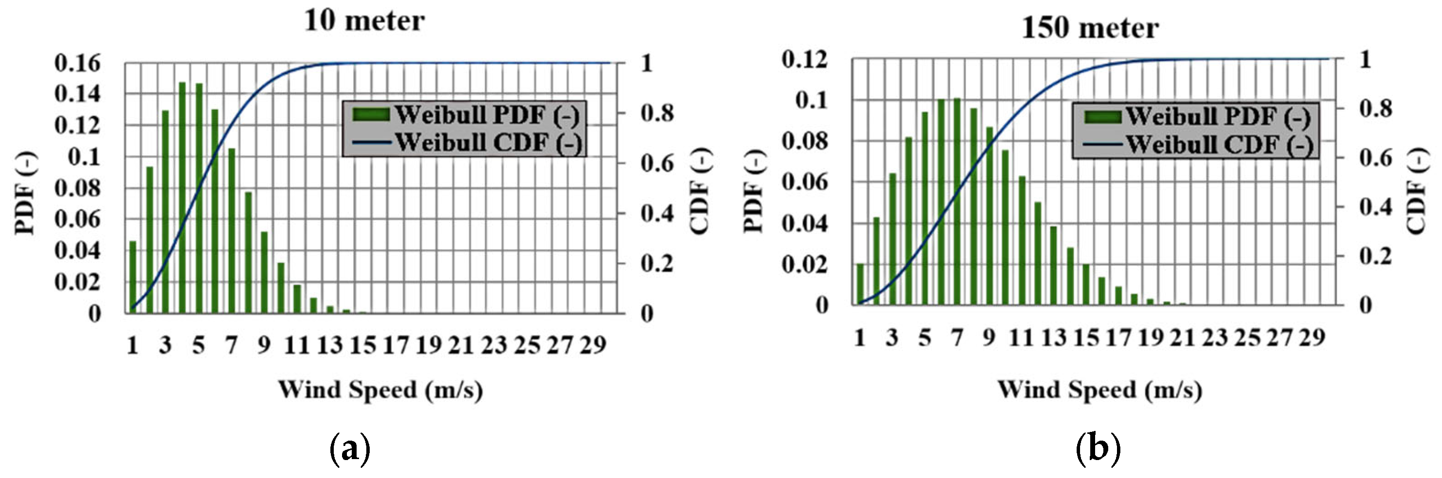
The Weibull algorithm explains the wind speed distribution in a very comprehensive and robust manner. Figure 3 show the wind speed distribution, as explained by the Weibull algorithm, at two different heights, i.e., 10 and 150 m (measured and extrapolated heights, respectively). Figure 3a confirms that the mean wind speed is nearly 5 m/s at 10 m height, as was also concluded from Table 2. Figure 3b shows that the mean wind speed is nearly 8 m/s at a 150 m height. The maximum wind speed reaches almost 21 m/s at a 150 m height as can also be concluded from Figure 3b.
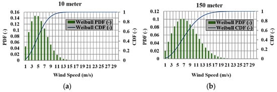
Figure 3.
Wind speed frequency: (a) 10 m; (b) 150 m (note: PDF denotes the probability density function and CDF the cumulative distribution function).
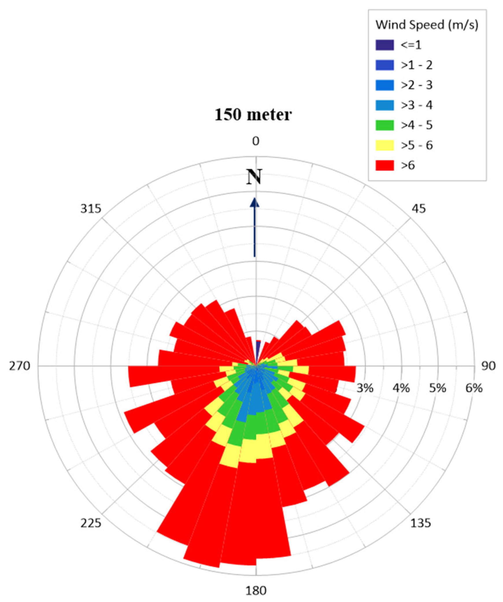
A wind rose is a type of figure that explains the wind speed distribution along with the wind direction. Figure 4 shows the wind rose diagram at the 150 m height of the specified wind data site. The wind speeds greater than 6 m/s usually come from the south and south-west directions. As shown in Figure 4, over 50% of the wind speeds are larger than 6 m/s with the maximum wind speed reaching up to approximately 21 m/s as also shown in Figure 3b.
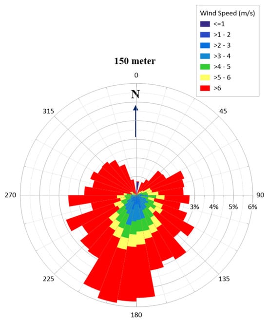
Figure 4.
Wind speed distribution according to wind direction.
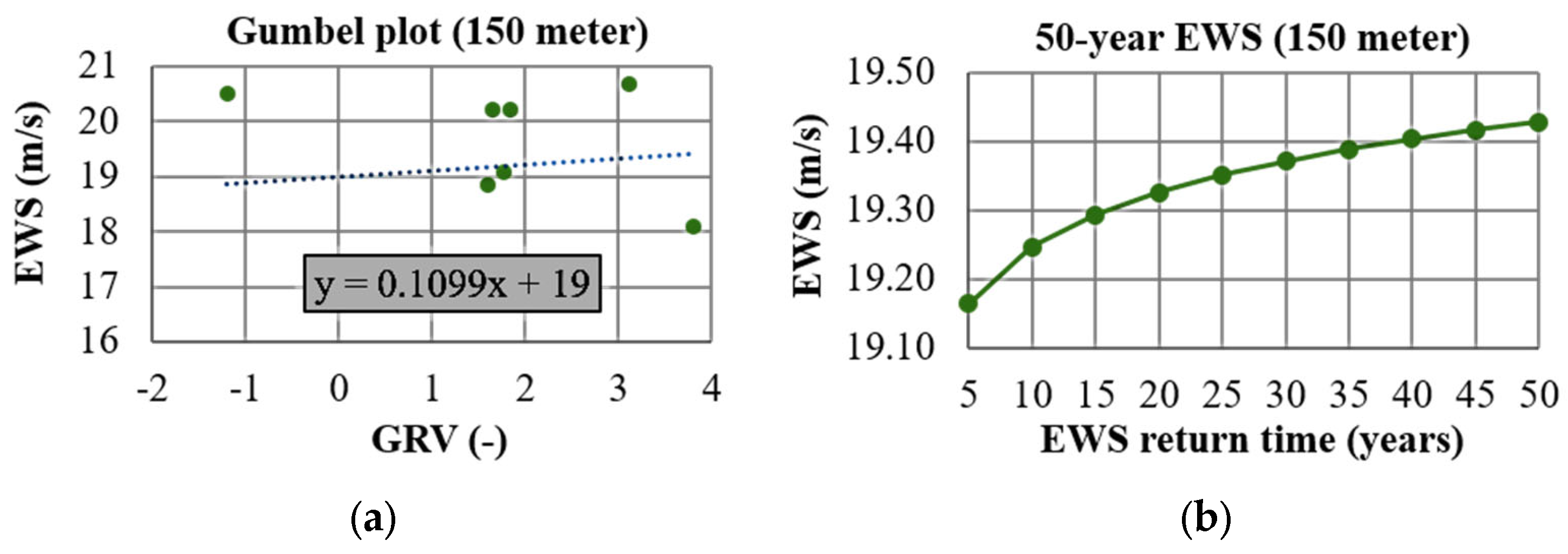
The wind data shown above were measured for seven years, i.e., from 2017 to 2023. But the actual wind power generation systems are usually designed for 20 years approximately. Therefore, the wind data for upcoming years must also be estimated using the available wind data measured at the reference hub height. In order to predict the wind data over the next 50 years, usually the Gumbel distribution is used [66]. More details about the Gumbel distribution and associated parameters can also be found in Reference [66]. Figure 5 shows the 50-year extreme wind speed (EWS) as predicted by the Gumbel distribution when applied to the available measured wind data sets. The 50-year EWS gust return can reach up to 20 m/s as shown in Figure 5b as well.
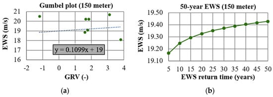
Figure 5.
Estimation of 50-year extreme wind speed: (a) Gumbel plot (note: GRV stands for Gumbel reduced variate); (b) 50-year EWS.
3.1.2. Hydro Characteristics
Similar to wind loads, hydro loads can also significantly affect the structural integrity of wind turbines (though wind loads are important for both, i.e., structure and power generation). But wind loads are most crucial in the rotor area, whereas hydro loads largely affect the monopile foundation and support structure. Hydro loads are much more impactive and impulsive than wind loads. Therefore, it is very important to determine the hydro loads in advance at the proposed wind farm site.
The present study uses the seven years (2017–2023) of measured data to determine the hydro loads at the chosen site, and the results are summarized in Table 3. The significant wave height (HS) is at a maximum during December and it is 7.4 m. Overall, HS is relatively higher during the winter season as compared to other seasons. The wave cycle (TP) on the other hand is at a maximum during the summer season and it is 11.9 s in April to be more specific. Both the significant wave height and wave cycle on the selected offshore site are generally on the higher level, as is also apparent from Table 3.
Table 3.
Measured wave data (monthly basis from 2017 to 2023).
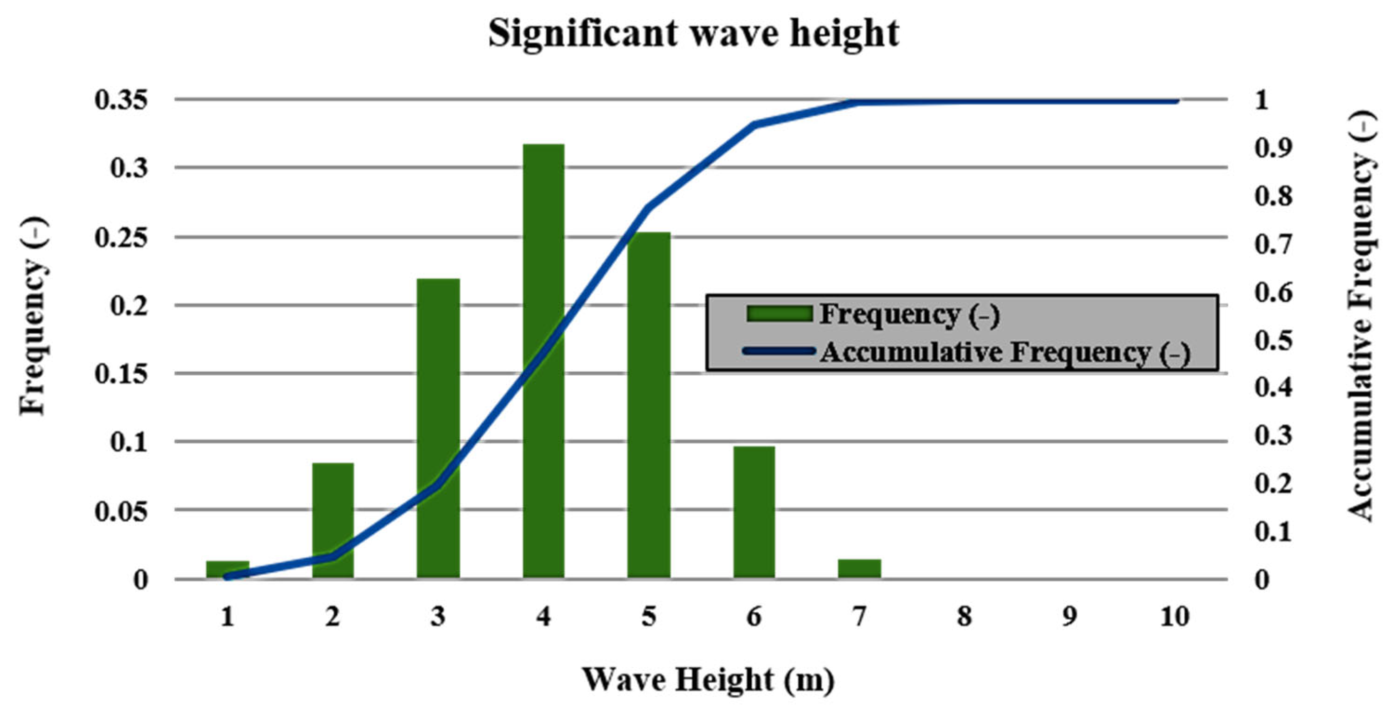
Figure 6 shows the significant wave height distribution in terms of frequency and accumulative frequency. It can be concluded from Figure 6 that 4 m is the most probable significant wave height which is quite high. It is also important to note that the maximum value of HS can reach up to as high as 7 m which can have a severe impact on the wind turbine tower and support structure as well.

Figure 6.
Significant wave height frequency distribution.
Similar to the wind rose diagram, a 360-degree chart explaining the significant wave height variation with the wave angle has also been prepared, and the results are shown in Figure 7. As can be observed in this figure, most of the waves are between 225 and 315 degrees of wave angle. The waves having a significant wave height above 6 m or so can be observed to be generally coming from the north-west side (315 degrees). Waves having a significant wave height between 2 and 3 m are the most frequent waves. Determining the appropriate wave angle along with the significant wave height is very significant for the structural health of an offshore wind turbine.
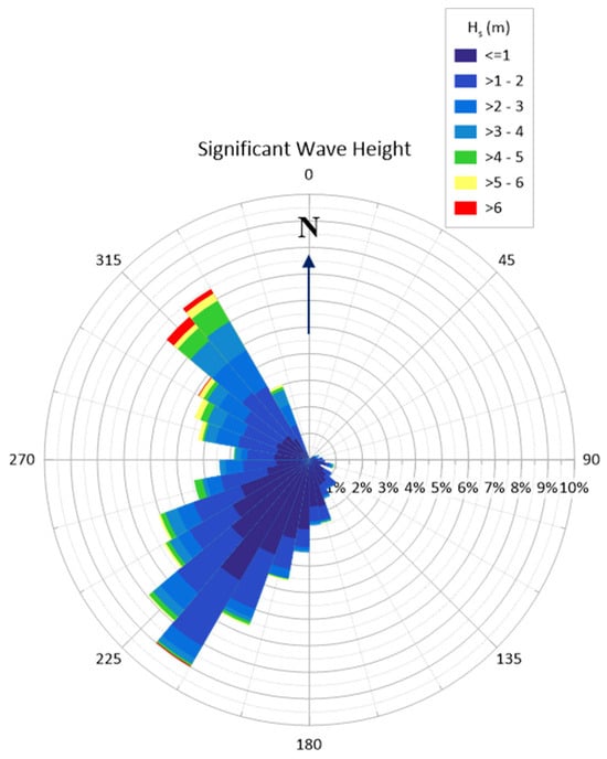
Figure 7.
Significant wave height distribution according to the wave direction.
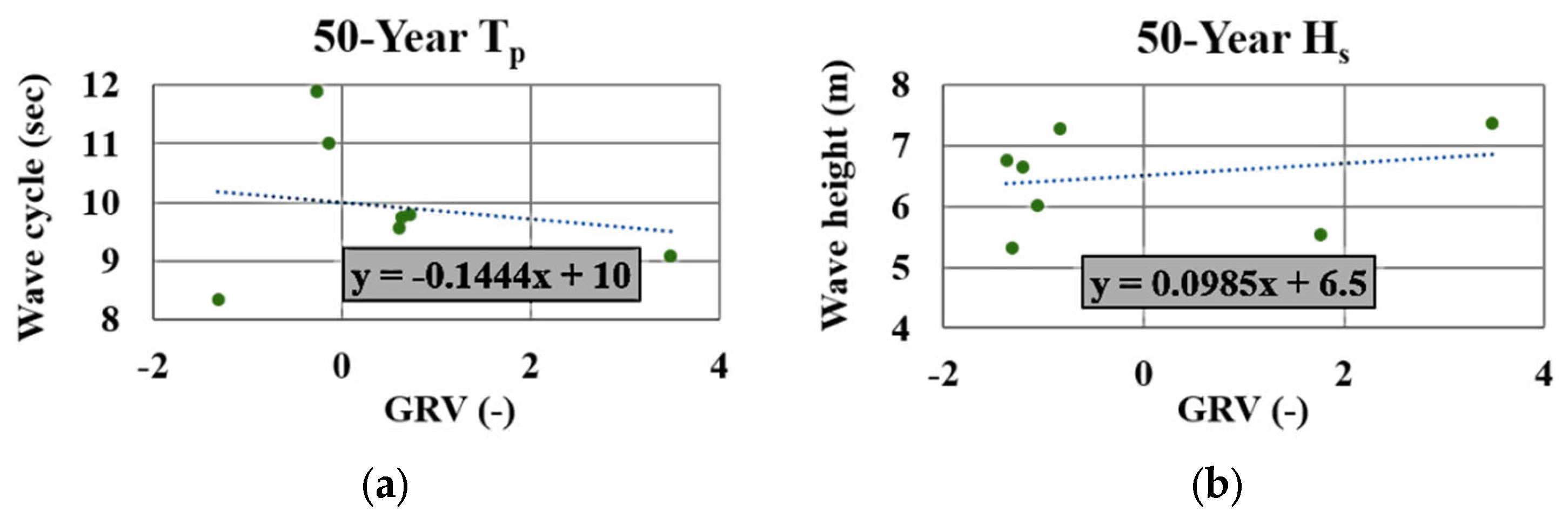
The prediction of a 50-year wave cycle (TP) and significant wave height (HS) also requires a lot of preciseness and available test or experimental data. Similar to EWS prediction, 50-year extreme TP and HS values can also be predicted using the Gumbel distribution. In this regard, Figure 8 shows the Gumbel plots for TP and HS which are usually drawn before predicting the 50-year extreme data. The slope of a Gumbel plot determines the level of extremeness that will be present in the future predicted 50-year wave data.
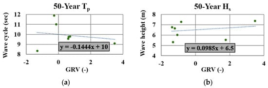
Figure 8.
Gumbel plots: (a) wave cycle; (b) significant wave height.
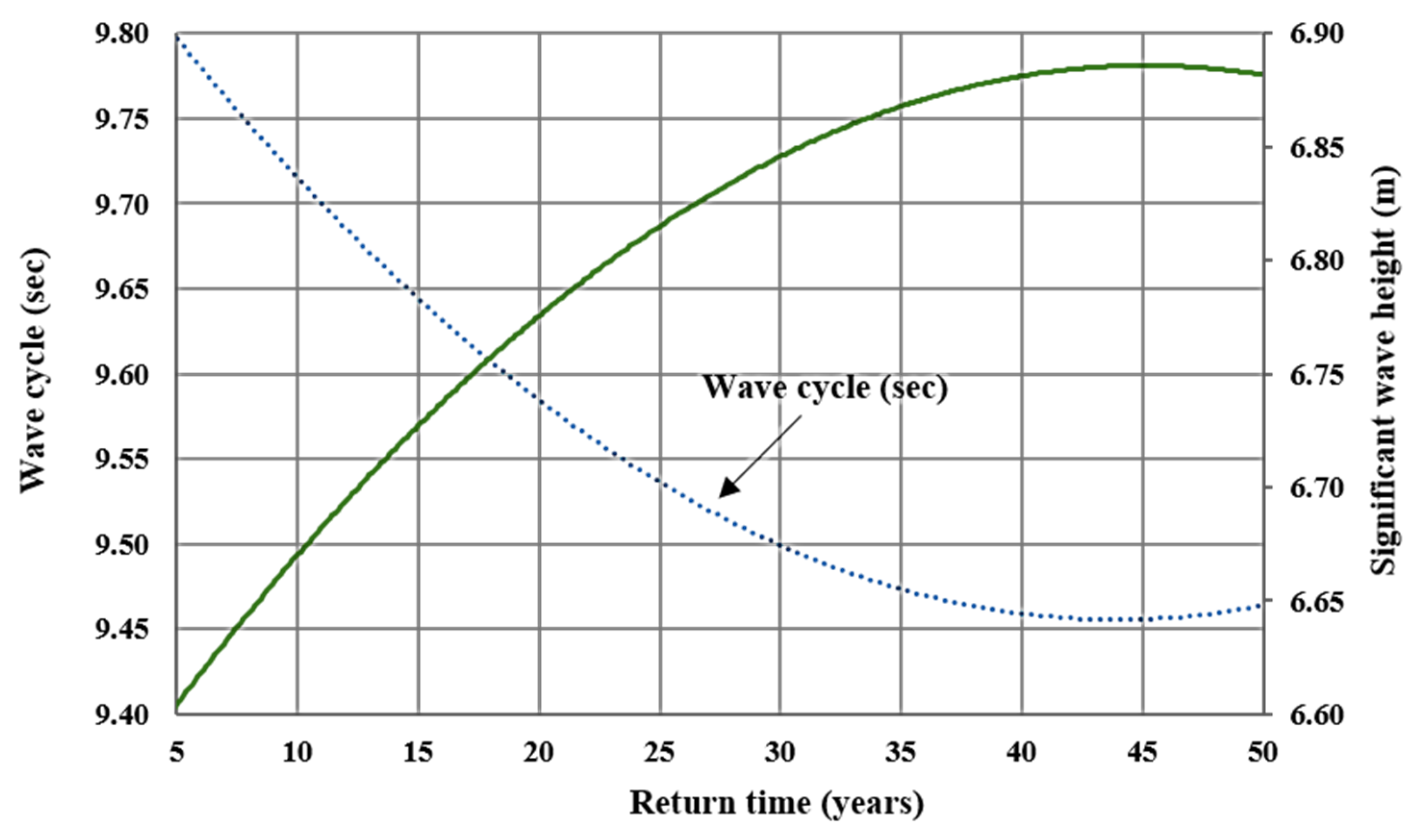
Figure 9 shows the 50-year extreme TP and HS wave data as predicted by the Gumbel distribution. The wave cycle is decreasing over time which means that more waves are expected to load on the wind turbine’s support structure in less time during future years. The decreasing trend of the wave cycle is due to the negative slope in the Gumbel plot as is also apparent from Figure 8a. As is apparent from Figure 9, the significant wave height is expected to range between 5 and 7 m during the next 50 years.
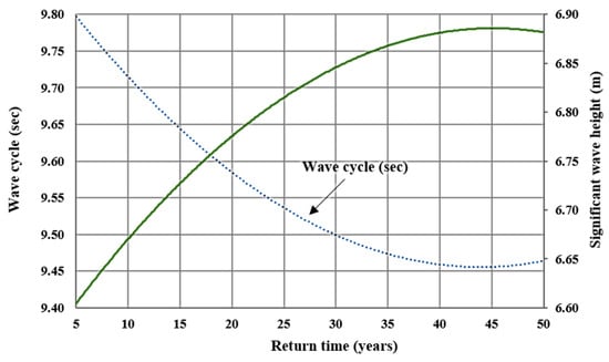
Figure 9.
Estimation of the 50-year extreme wave cycle and significant wave height.
3.2. Performance Coefficients
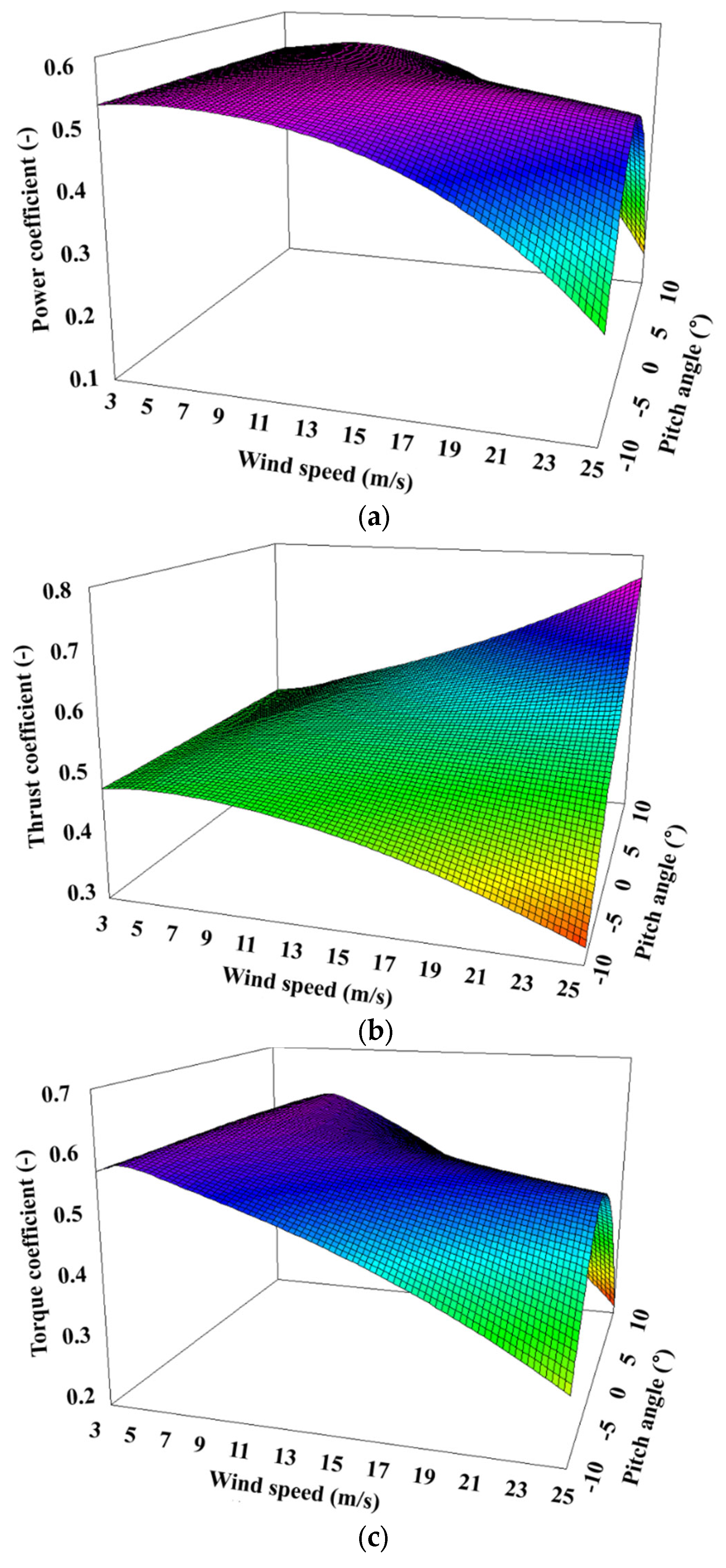
Before analyzing the structural and energy production performance of the wind turbine in specific conditions, it is important to determine the range of operating variables at which an optimized power performance is achieved. In order to fulfil this goal, Figure 10 have been prepared. These figures are 3D contour plots of three important parameters, i.e., power, thrust, and the torque coefficient of the wind turbine against the wind speed and blade pitch angle, respectively.
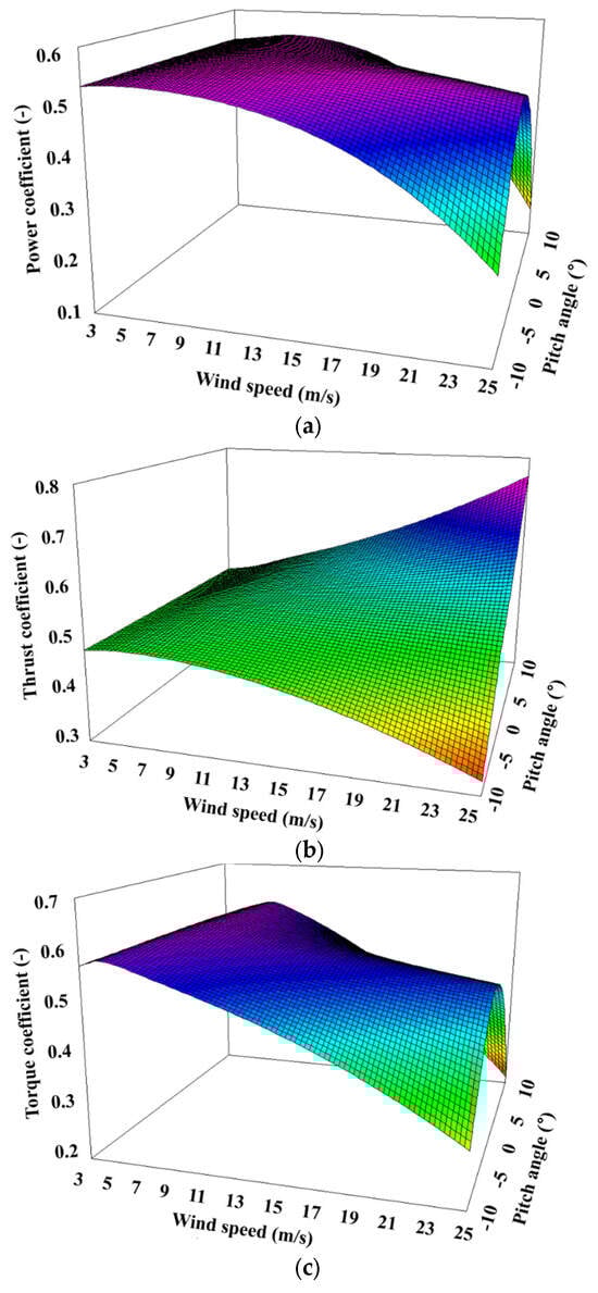
Figure 10.
Wind turbine performance coefficients against wind speed and blade pitch angle: (a) power coefficient; (b) thrust coefficient; (c) torque coefficient.
As can be observed in Figure 10, the optimum pitch angle and wind speed are 0 degrees and 11 m/s, respectively. The power coefficient is slightly higher at a pitch angle of 10 degrees and a wind speed of almost 11 m/s. But it can be observed in Figure 10b as well that the thrust coefficient is at a maximum at a pitch angle of 10 degrees, and it is the minimum at a pitch angle of −10 degrees. Ideally, the thrust coefficient should be minimum in order to avoid the impulsive aerodynamic loads which can cause severe damage to all components of the wind turbine including the rotor, tower, and support structure.
But it can be observed in Figure 10a,c that both the power and torque coefficients are at a minimum at −10 degrees, as well as 10 degrees of pitch angle, specifically at higher wind speeds. Therefore, it is a trade-off between power performance and structural health when it comes to choosing an optimum value or range of pitch angle. In such a scenario, a middle value of pitch angle would be more appropriate at which the thrust coefficient is not too high and neither the power nor torque coefficients are very low. Therefore, such a pitch angle is 0 degrees, which will be considered as an optimum value and will be used for analysis in rest of this study.
Along with determining the optimum pitch angle, it is also very important to determine an optimum range of wind speed where the power or torque coefficient are at a maximum along with minimum thrust coefficients. Figure 10 again is greatly beneficial for this purpose too. After analyzing Figure 10, it can be concluded that a wind speed range of 8 to 14 m/s is best-suited for analyzing the energy and structural performance of the wind turbine. This range of wind speed is only chosen because all three coefficients, i.e., power, thrust, and the torque coefficient, are optimized according to the same criteria as defined for optimizing the blade pitch angle.
3.3. Structural Loads
3.3.1. Monopile Foundation
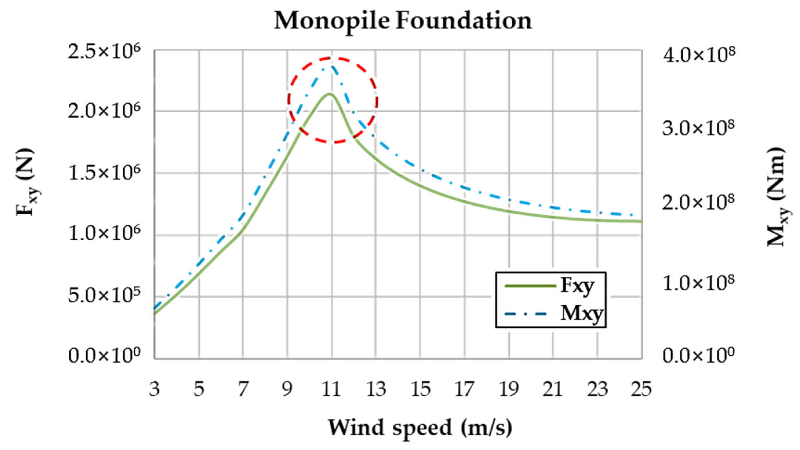
From here onwards, the main results and analysis of the present study will be discussed in detail. The monopile foundation of a fixed-type offshore wind turbine receives the most loads and moments. The present study uses the simple monopile foundation as explained above. Figure 11 shows the two-directional resultant reaction forces and moments acting on the monopile foundation of the wind turbine against the full wind speed scale considered in the present study.
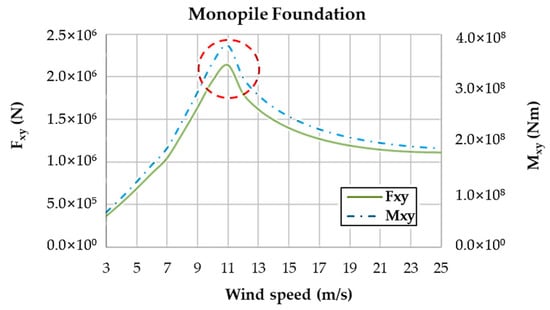
Figure 11.
Forces and moments on the monopile foundation according to wind speed (note: loads occur at a point which is 45 m above the monopile foundation base (joint point of the monopile foundation top and the sub-structure bottom as shown in Figure 2b as well). Please also note that the red-dashed circular area is the most critical due to maximum forces and moments).
As can be observed in Figure 11, the resultant moment acting on the monopile foundation is much larger in magnitude as compared to the resultant acting force (the x- and y-directions have already been defined above). In this figure, exactly the same pattern of wind speed optimization can be observed again, exactly as concluded above, i.e., 11 m/s is the most critical wind speed. The reaction forces increase until 11 m/s after which both forces start to drop rapidly. It should be noted that at 11 m/s, the power coefficient was also at a maximum as concluded above. From now onwards, concluding from Figure 11, it is decided to carry out the further analysis in the present study only between 8 and 14 m/s. It is worth mentioning that the results shown in Figure 11 are prepared at 0 degrees of blade pitch angle.
Table 4 summarizes the peak forces and moments on the monopile foundation at the selected critical wind speeds.
Table 4.
Force and moment matrix.
3.3.2. Tower
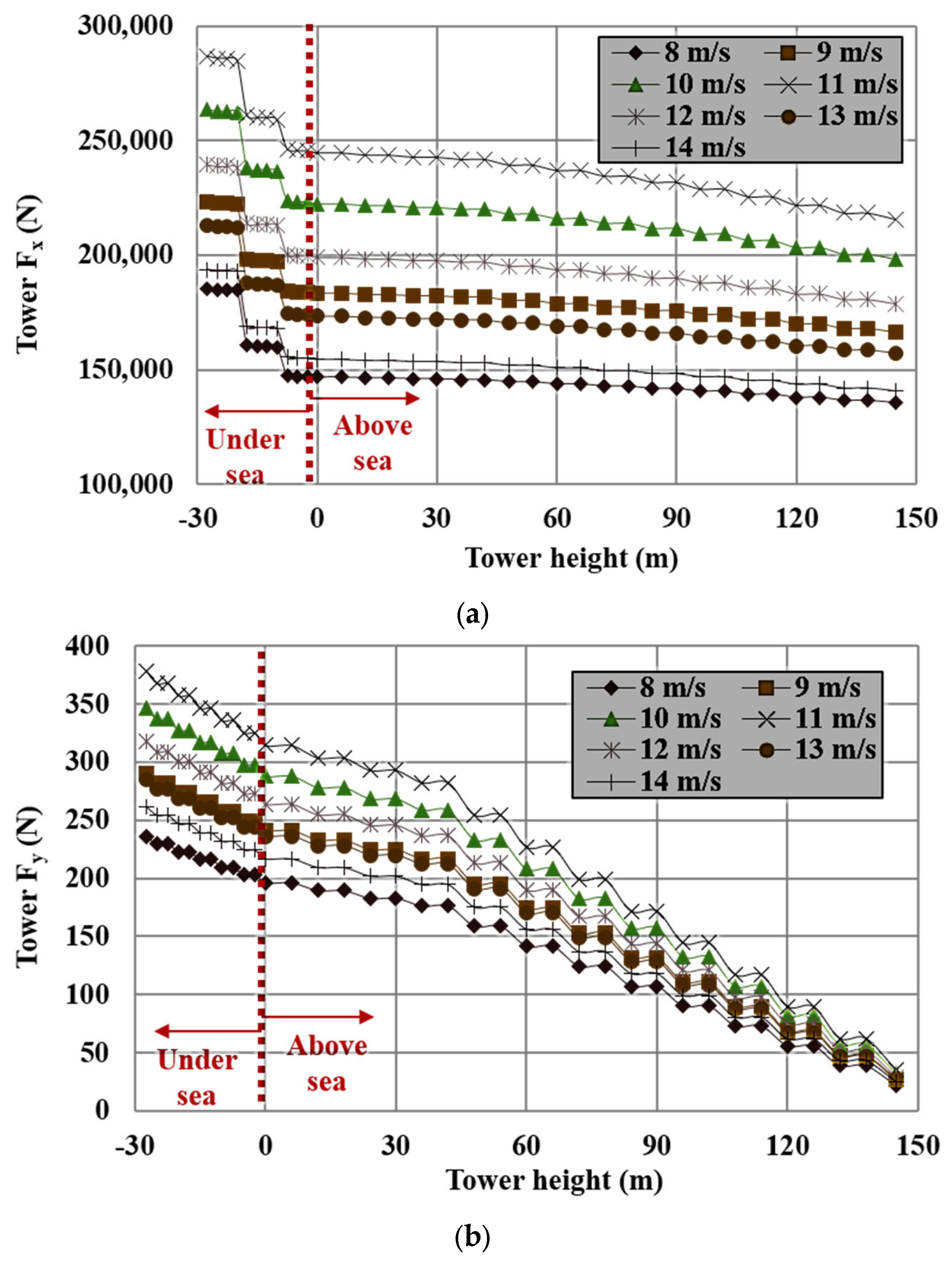
Figure 12 shows the x and y-direction forces acting on the tower, and the results are shown against the tower height. The tower can be divided into two parts: one which is under the sea (30 m), and the other one which is above-sea standing in the air (150 m). The results are prepared only for 8 to 14 m/s of wind speed as discussed above. The tower cross-section is circular and its diameter decreases from bottom (foundation) to top (nacelle position). The exact dimensions of the tower and other geometrical properties can be found on the NREL website.
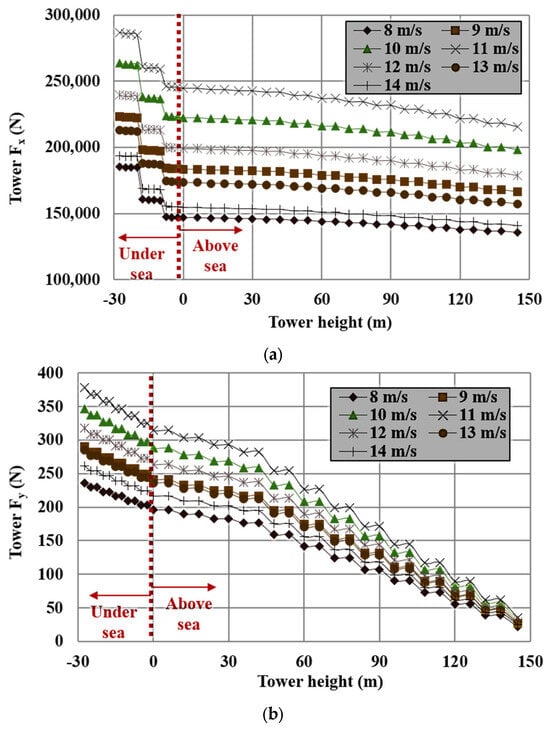
Figure 12.
Forces on the tower according to tower height: (a) Fx; (b) Fy.
There are many interesting and distinct phenomena that can be noticed in Figure 12. First, the x-direction force magnitude is much higher than the y-direction force magnitude. Second, the maximum force acting on the tower is almost 300 kN which is approximately six times less than the maximum force acting on the monopile foundation. Third, the maximum force acting on the tower is at the bottom. Fourth, the maximum force occurs at 11 m/s of wind speed in both cases, i.e., the x- and y-directions. Fifth, the two forces (x and y) are reducing from bottom to top. Sixth, the undersea forces in Figure 12a,b are much larger than the forces acting on that part of tower which is in the air. The reason for the undersea forces being larger than the above-sea forces is that the undersea forces are combinedly due to rotor aerodynamics and tower hydro forces, whereas the above-sea forces are due to rotor aerodynamics combined with tower aerodynamics forces. In general, the hydro load is much more than the aero load. Seventh, the hydro forces (undersea) acting on the tower are decreasing sharply with a significant step size, whereas the aero forces (above-sea) are smoothly diminishing with tower height. The possible reason might be wave currents, which change their amplitude and frequency over time. Therefore, waves colliding with the tower have different characteristics over time as is also apparent from Figure 12.
3.3.3. Blades
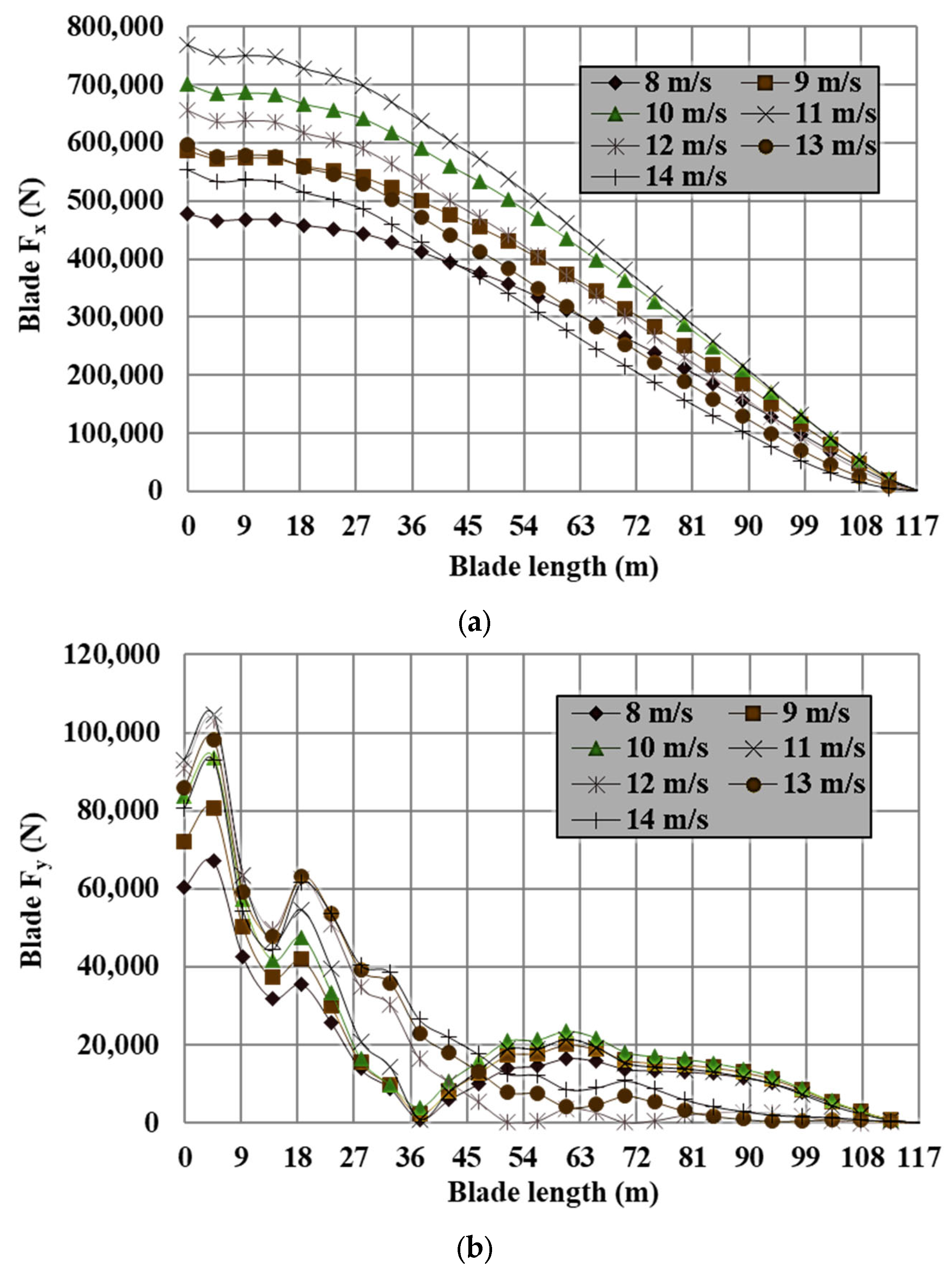
Similar to the forces acting on the tower, the forces acting on blades have also been numerically estimated, and the results are shown in Figure 13. Unlike the tower forces, the force experienced by the blades in the y-direction is also quite significant. Although the y-direction force is almost seven times less than the x-direction force, it is still very impactive. The forces are calculated over the entire blade length at 8 to 14 m/s of wind speed.
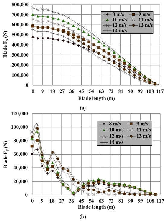
Figure 13.
Forces on the blade according to blade length: (a) Fx; (b) Fy.
Both forces (x and y) decrease with blade length from the hub to the tip of the blade. The maximum x-direction force is nearly 769 kN, whereas the maximum y-direction force is almost 105 kN. Both maximum forces correspond to 11 m/s of wind speed and are acting on the bottom of the blade attached to the hub. The maximum force acting on the blade is nearly three times larger than the maximum force acting on the tower, and it is 2.5 times less than the maximum force acting on the monopile foundation.
It is important to mention that the blade forces are due to the generation of two fundamental aerodynamics forces, i.e., lift and drag. The x-direction force on the blade is due to drag, whereas the y-direction force on the blade is due to lift. From Figure 13, it can be concluded that the drag force is almost eight times higher than the lift force. Both drag and lift largely depend on the blade pitch angle because the blade pitch angle controls how much wind will pass over the surface of the blades. That is why the blade pitch angle was first optimized as described above earlier. The drag force on the blade is generally more complex and transient as compared to the lift force. The forces acting on the blade are the most important and effective forces as compared to the rest of the forces acting on any other component of the wind turbine because the blade forces affect the structure of the wind turbine and all its components from top to bottom. For example, the x-direction force acting on the tower is partially generated due to the blades’ x-direction force. Similarly, y-direction blades’ force (lift) also increases the weight of the rotor (though this aerodynamic weight changes with time and wind speed). It should be noted that the results shown in Figure 13 and Figure 14 are only for a single blade.
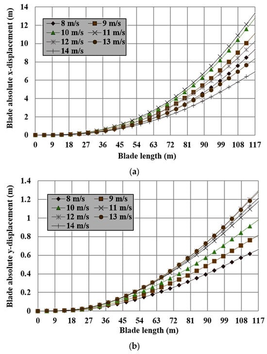
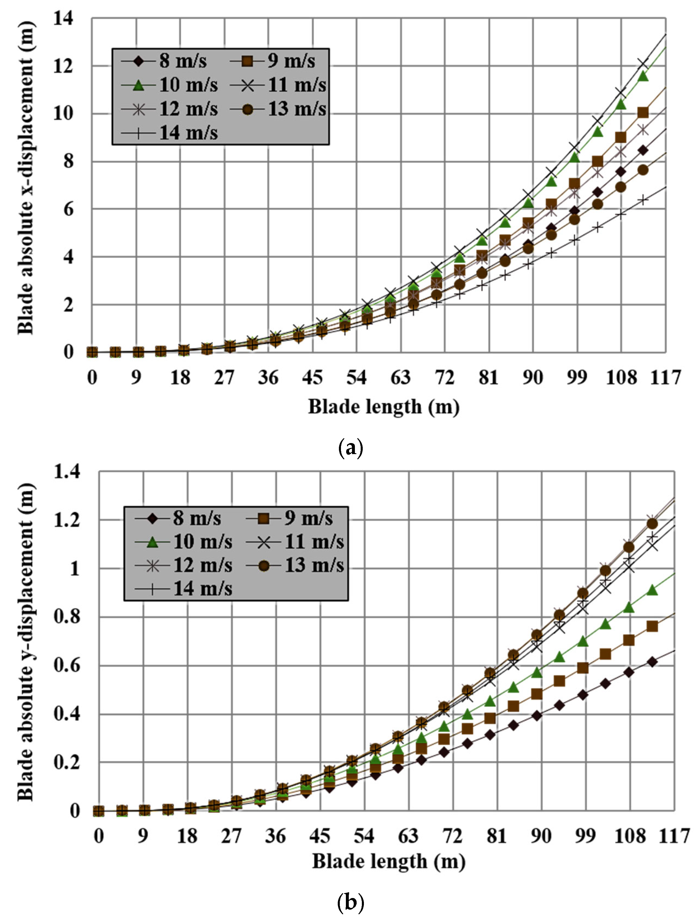
Figure 14.
Blade absolute displacement according to blade length: (a) x-displacement; (b) y-displacement.
Figure 14 show the absolute x and y-direction blade displacement alongside blade length for 8 to 14 m/s of wind speed. Both displacements are increasing with blade length for all wind speeds due to reduced blade mass over its length. The maximum x-direction displacement is nearly 13 m on the tip of the blade at 11 m/s of wind speed. This maximum value is nearly 10 times more than the y-direction displacement on the blade. The reason behind such a large difference between the x- and y-direction displacements is the corresponding large difference between the drag and lift forces as concluded and described above as well.
3.4. Energy Production
3.4.1. Monthly Basis
Along with loading and displacement analysis, analysis of the energy production from a wind turbine is also critically important. In this regard, Figure 15, Figure 16, Figure 17 and Figure 18 have been prepared to estimate the energy production from the wind turbine on a monthly, seasonal, and annual basis, respectively. These results are computed using the wind data measured at the mentioned site from 2017 to 2023. Seven years of measured wind data can be considered as a medium level of available wind information at the selected site. Therefore, all energy results presented in Figure 15, Figure 16, Figure 17 and Figure 18 can be considered as generalized at the mentioned test site. Almost the same amount of energy production can even be assumed for many years to come (let’s assume 20 years).
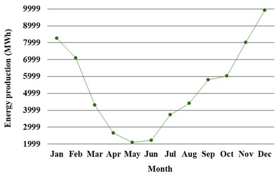
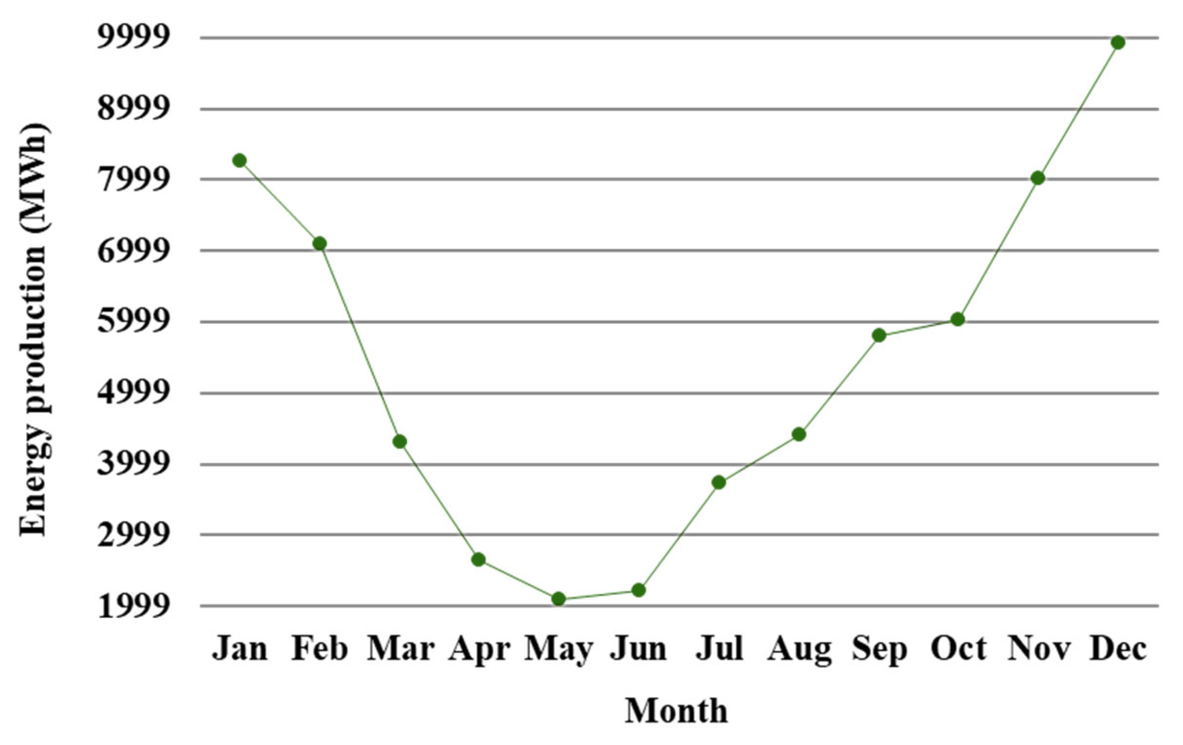
Figure 15.
Monthly energy generation (in MWh).
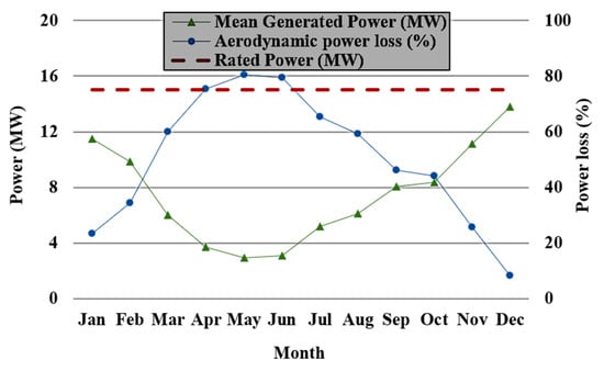
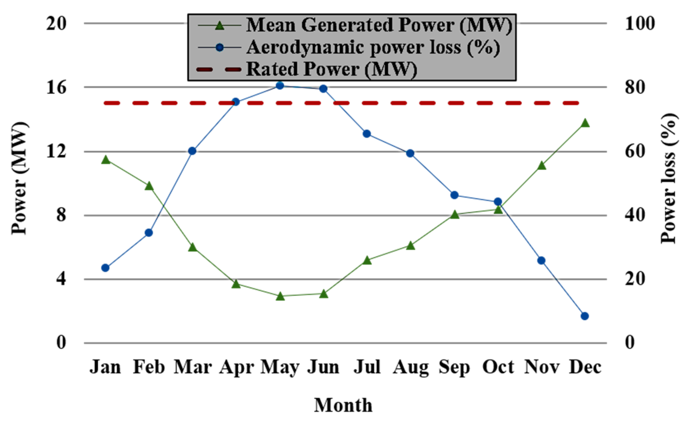
Figure 16.
Monthly average power production (in MW).
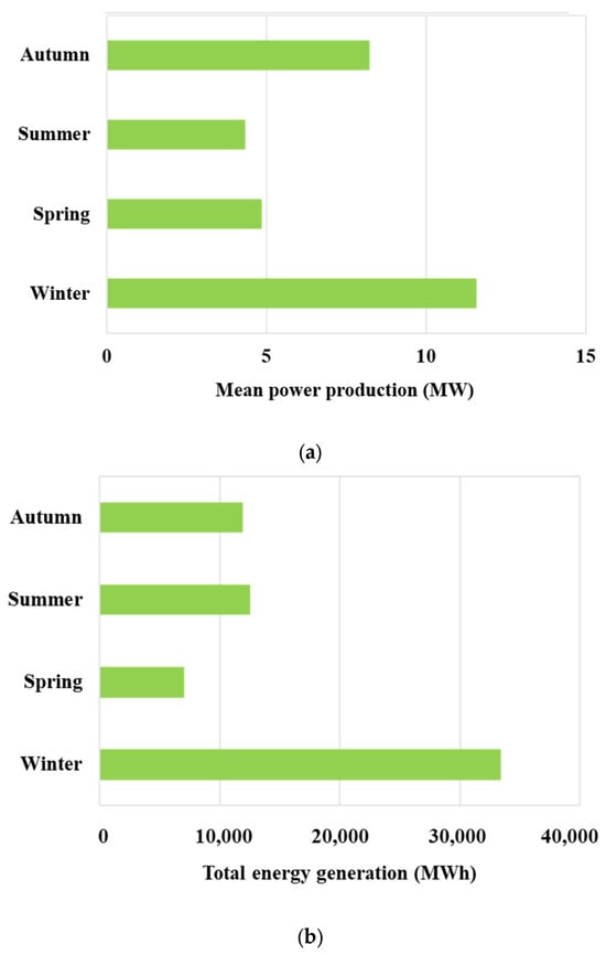
Figure 17.
Seasonal energy analysis: (a) mean power production; (b) total energy generation.
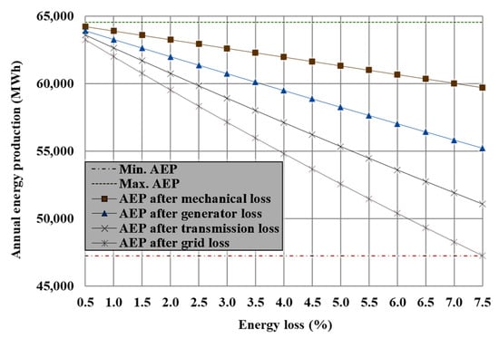
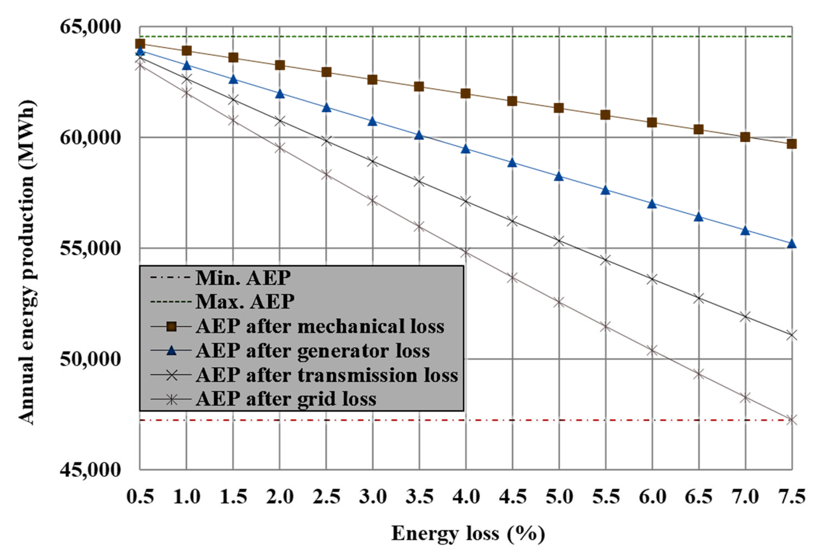
Figure 18.
Annual energy production including different loss rates.
Figure 15 shows the energy production in MWh on a monthly basis. A total of 10 GWh energy can be produced only during the month of December, and this is the highest energy production as compared to any other month. The highest wind speed during December is the obvious reason behind the maximum energy production. But another minor reason is the relatively high momentum of wind during December due to the low air temperature and high air density. The lowest energy production is during May, which is almost 2 GWh.
Figure 16 shows the average power production from the wind turbine (in MW) on a monthly basis. It should be noticed that Figure 15 presents the accumulative wind energy generation, whereas Figure 16 presents the average power production which was used to estimate energy generation. Figure 16 reveals the same pattern as can be observed in Figure 15 as well. This figure also shows the monthly aerodynamic loss which is nothing but the difference between the wind turbine rated power and the average power produced. During May only, a maximum of 80% power loss can be noticed. During December, the wind turbine produces power on an average scale of 14 MW which is the highest among all of the months.
3.4.2. Season Basis
Along with monthly energy production estimations, another important parameter that needed to be estimated was the seasonal energy production from the wind turbine. Figure 17 shows the mean power production and accumulative energy generation during the four seasons, i.e., autumn, summer, spring, and winter, respectively. Figure 17 concludes that winter is the best season for harvesting energy at the test site using the NREL-IEA 15 MW wind turbine. During the entire winter season, the wind turbine produces power at the rate of roughly 12 MW which is the highest among all seasons. It should be clarified that the four seasons have been defined as follows:
- Autumn: September to October;
- Summer: May to August;
- Spring: March to April;
- Winter: November to February.
A detailed analysis of Figure 17 reveals that although spring is not the season of minimum power production (Figure 17a), the energy production is the lowest during this season (Figure 17b). This is because of the fact that Figure 17a is based on the average data, whereas Figure 17b is based on accumulative data integrated over the entire time period of the season. Figure 17b shows less energy generation during spring only due to the fact that the spring season has only two months as defined above. Therefore, it can be concluded that summer is the season which has the lowest wind potential compared to the other seasons as also apparent from Figure 17a.
3.4.3. Annual Energy Production (AEP)
Lastly, the most important parameters related to wind turbine power production, i.e., AEP, have also been estimated and the results are presented in Table 5. The wind turbine will produce a total of 64.54 GWh of aerodynamic energy at the rate of 7.47 MW annually. It is nearly 50% of the rated power of the chosen wind turbine model.
Table 5.
Annual energy production.
Figure 18 presents very interesting scenarios about the net power production and energy loss rates. Actually, the AEP mentioned in Table 5 is purely mechanical or aerodynamic power. It does not include any losses or other factors. That is the maximum possible energy that can be generated. But the net AEP includes losses of many types, e.g., generator and grid loss, etc. Figure 18 comprehensively shows the net AEP after including all types of losses. The range of each loss has been taken from 0.5 to 7.5%. The minimum possible energy that can be stored in the electric grid is around 47 GWh which is almost 73% of the maximum possible AEP. This minimum possible AEP has been estimated by considering a constant value for each loss rate of 7.5%, which is the maximum loss rate considered in the present study.
4. Discussion and Future Recommendations
The results presented in the current study are very useful for future wind farms’ planners especially and the research community in general. This study also provides a comprehensive framework for analyzing the performance of large-scale wind turbines in a multi-dimensional manner. The present work is based on numerical calculations; therefore, the results should be verified using other experimental and/or published results. There are very few experimental results available in this regard, e.g., [67,68]. The study conducted by Nicole et al. [67] can be used very well for this purpose. The experimental x-direction force on the tower top, as mentioned in this lab-scale mock-up study, is nearly 240 kN, whereas it is 225 kN in the current work (a 6.25% absolute difference). The results of the present study are also verified by a study conducted by Fritz et al. [68].
The long-term and accurate determination of wind speed and direction at the planned wind farm site is very important for the optimal sitting of wind turbines. The current study used the measured wind data for analyzing the wind turbine performance, and the wind characteristics are very similar to the usual Korean wind conditions as mentioned in previous works [69,70,71]. Similarly, wave characteristics play an important role in determining the fatigue and remaining useful life of the tower and monopile foundation. As mentioned by Yu et al. [72] in an experimental study, even the smallest waves with a wave height of 28 mm and a wave cycle of 1 s can produce tower displacement.
It should also be mentioned that the structural results presented in the current work were computed at optimized operating conditions in terms of the maximum power and torque coefficient. If the conditions are different, then the results (specifically the structural results) might not have been identical to the current scenario. The pitch angle plays a vital role, not only in controlling the power production of the wind turbine but also for the foundation and tower loads which largely depend on it. In the present study, a pitch angle of 0° was chosen because of the maximum power production and lower loads on the structure. However, for different scenarios and situations, where the final goals might be different, a different set of operating conditions must be optimized. The study conducted by Papi and Bianchini [73] mentioned pitch angle optimization for an IEA 15 MW reference wind turbine. However, they only optimized the pitch angle for different wind speeds rather than optimizing for torque or power production as performed in the current study. They also found that 10 or 11 m/s is the most critical wind speed for this specific wind turbine, as is also one of the conclusions of the current work. Similarly, a very recent paper published by Lapa et al. [74] also found that the maximum blade displacement was 15.0 (flap-wise) and 1.5 (edgewise) meters, estimated using the prestigious GIRAFFE program. This also validates and strengthens the outcomes of the current study, where it is 13.5 (flap-wise) and 1.3 (edgewise) meters, respectively. Therefore, in both of these studies, the blade flap-wise displacement is nearly 10% of the blade length which is 117 m as prescribed by IEA.
Another important discussion point is that this study investigated maximum average wind speed values ranging from 12.27 m/s to 14.01 m/s, representing a non-extreme wind loading scenario. Climate change and global warming in combination with other underlying meteorological phenomena are known to increase the intensity of tropical cyclones.
Some recent typhoons making landfall in South Korea with their wind speeds at 10 m height are as follows:
- Typhoon Khanun (2023): Winds up to 43.89 m/s.
- Typhoon Hinnamnor (2022): Maximum sustained winds around 43.61 m/s.
- Typhoon Maysak (2020): Maximum sustained winds around 43.06 m/s.
- Typhoon Haishen (2020): Winds up to 44.44 m/s.
More studies on the structural design of wind turbine foundations are needed to investigate these new normal extreme wind conditions. A foundation designed to 14.01 m/s may not withstand typhoon wind forces.
Also, since 2021, many manufacturers of wind turbines (including Siemens-Gamesa, Vestas, General Electric, and others) have obtained the certification of IEC T-class typhoon-proof turbines [75,76,77]. Future studies may also investigate the state of art in commercial wind turbines.
Finally, the jacket foundation design may be better suited for T-class wind conditions [77].
Further structural analysis research is required considering alternative types of foundation.
5. Conclusions
There are very few studies available in the literature which have analyzed both the power and structural performance of large-scale horizontal axis wind turbines such as the NREL-IEA 15 MW wind turbine. The present work analyzes the energy production and structural performance of the NREL-IEA 15 MW wind turbine using measured wind and hydro data. First of all, optimum operating ranges are determined in terms of wind speed and blade pitch angle to maximize the power coefficient. Then, at these optimum ranges, a detailed breakdown of the forces and moments acting on different components of the wind turbine is being presented. It was found that 9 to 12 m/s of wind speed is most suitable for this wind turbine as the power coefficient is at a maximum, as well as the loads being at a minimum on all components. The loads found to be at a minimum due to the optimized blade pitch angle. The force on the monopile foundation is found to be at a maximum and it corresponds to nearly 2000 kN. The maximum blade force is nearly 700 kN, whereas on the tower it is almost 250 kN. The maximum force acting on the tower occurs at a point which is found to be undersea, whereas above-sea the maximum force on the tower is nearly 20% less than the undersea maximum force.
Using field-measured wind data, the power production performance of the wind turbine is also analyzed on a monthly, seasonal and annual basis. The winter season, in particular the month of December, is found to be the optimum period for maximum energy harvesting, which corresponds to a maximum of 10,000 MWh; in contrast, May is found to be the least energy productive month as only 2000 MWh of energy can be produced during this month. The total annual energy production corresponds to over 64,000 MWh (the exact number is 64,540 MWh).
Author Contributions
Conceptualization, S.A. and D.L.; methodology, S.A.; software, S.A.; validation, S.A. and H.P.; formal analysis, S.A.; investigation, S.A.; resources, S.A.; data curation, D.L.; writing—original draft preparation, S.A.; writing—review and editing, D.L.; visualization, H.P.; supervision, D.L.; project administration, D.L.; funding acquisition, D.L. All authors have read and agreed to the published version of the manuscript.
Funding
1. This work was supported by the Human Resources Development of the Korea Institute of Energy Technology Evaluation and Planning (KETEP) grant funded by the Korean government Ministry of Trade, Industry & Energy (No. 20214000000180). 2. This research was supported by the Basic Science Research Program through the National Research Foundation of Korea (NRF) funded by the Ministry of Education (NRF2021R1A6A1A03045185).
Institutional Review Board Statement
Not applicable.
Informed Consent Statement
Not applicable.
Data Availability Statement
The data presented in this study are available on request from the corresponding author.
Acknowledgments
The authors would like to express their gratitude to KMA for providing the wind and wave data sets.
Conflicts of Interest
The authors declare no conflicts of interest.
References
- Sánchez, S.; López-Gutiérrez, J.S.; Negro, V.; Esteban, M.D. Foundations in offshore wind farms: Evolution, characteristics and range of use. Analysis of main dimensional parameters in monopile foundations. J. Mar. Sci. Eng. 2019, 7, 441. [Google Scholar] [CrossRef]
- Dromant Bellver, B. An EU Strategy to Harness the Potential of Offshore Renewable Energy for a Climate Neutral Future. Available online: https://roderic.uv.es/items/9fdb5f40-edbd-410e-912c-25d8234547a1 (accessed on 12 July 2024).
- Bento, N.; Fontes, M. Emergence of floating offshore wind energy: Technology and industry. Renew. Sustain. Energy Rev. 2019, 99, 66–82. [Google Scholar] [CrossRef]
- Duffy, A.; Hand, M.; Wiser, R.; Lantz, E.; Dalla Riva, A.; Berkhout, V.; Stenkvist, M.; Weir, D.; Lacal-Arántegui, R. Land-based wind energy cost trends in Germany, Denmark, Ireland, Norway, Sweden and the United States. Appl. Energy 2020, 277, 114777. [Google Scholar] [CrossRef]
- Li, X.; Wu, Z.; Su, D.; Zhang, L. Reliability analysis of offshore monopile foundations considering multidirectional loading and soil spatial variability. Comput. Geotech. 2024, 166, 106045. [Google Scholar] [CrossRef]
- Shields, M.; Beiter, P.; Nunemaker, J.; Cooperman, A.; Duffy, P. Impacts of turbine and plant upsizing on the levelized cost of energy for offshore wind. Appl. Energy 2021, 298, 117189. [Google Scholar] [CrossRef]
- Kikuchi, Y.; Ishihara, T. Upscaling and levelized cost of energy for offshore wind turbines supported by semi-submersible floating platforms. J. Phys. Conf. Ser. 2019, 1356, 012033. [Google Scholar] [CrossRef]
- Veers, P.; Dykes, K.; Lantz, E.; Barth, S.; Bottasso, C.L.; Carlson, O.; Clifton, A.; Green, J.; Green, P.; Holttinen, H.; et al. Grand challenges in the science of wind energy. Science 2019, 366, eaau2027. [Google Scholar] [CrossRef]
- Ren, Z.; Verma, A.S.; Li, Y.; Teuwen, J.J.; Jiang, Z. Offshore wind turbine operations and maintenance: A state-of-the-art review. Renew. Sustain. Energy Rev. 2021, 144, 110886. [Google Scholar] [CrossRef]
- Jiang, Z.; Gao, Z.; Ren, Z.; Li, Y.; Duan, L. A parametric study on the final blade installation process for monopile wind turbines under rough environmental conditions. Eng. Struct. 2018, 172, 1042–1056. [Google Scholar] [CrossRef]
- Chitteth Ramachandran, R.; Desmond, C.; Judge, F.; Serraris, J.J.; Murphy, J. Floating offshore wind turbines: Installation, operation, maintenance and decommissioning challenges and opportunities. Wind Energy Sci. Discuss. 2021, 2021, 903–924. [Google Scholar]
- Bak, C.; Zahle, F.; Bitsche, R.; Kim, T.; Yde, A.; Henriksen, L.C.; Hansen, M.H.; Blasques, J.P.; Gaunaa, M.; Natarajan, A. The DTU 10-MW Reference Wind Turbine; Danish Wind Power Research: Fredericia, Denmark, 2013. [Google Scholar]
- Sieros, G.; Chaviaropoulos, P.; Sørensen, J.D.; Bulder, B.H.; Jamieson, P. Upscaling wind turbines: Theoretical and practical aspects and their impact on the cost of energy. Wind Energy 2012, 15, 3–17. [Google Scholar] [CrossRef]
- Ashuri, T. Beyond Classical Upscaling: Integrated Aeroservoelastic Design and Optimization of Large Offshore Wind Turbines; NARCIS: The Hague, The Netherlands, 2012. [Google Scholar]
- Leimeister, M.; Bachynski, E.E.; Muskulus, M.; Thomas, P. Rational upscaling of a semi-submersible floating platform supporting a wind turbine. Energy Procedia 2016, 94, 434–442. [Google Scholar] [CrossRef]
- Ferri, G.; Marino, E.; Borri, C. Optimal dimensions of a semisubmersible floating platform for a 10 MW wind turbine. Energies 2020, 13, 3092. [Google Scholar] [CrossRef]
- Butterfield, S.; Musial, W.; Jonkman, J.; Sclavounos, P. Engineering Challenges for Floating Offshore Wind Turbines; National Renewable Energy Lab. (NREL): Golden, CO, USA, 2007.
- Jonkman, J.M. Loads Analysis of a Floating Offshore Wind Turbine Using Fully Coupled Simulation; National Renewable Energy Lab. (NREL): Golden, CO, USA, 2007.
- Jonkman, J. Influence of control on the pitch damping of a floating wind turbine. In Proceedings of the 46th AIAA Aerospace Sciences Meeting and Exhibit, Reno, NV, USA, 7–10 January 2008; p. 1306. [Google Scholar]
- Liu, Y.; Li, S.; Yi, Q.; Chen, D. Developments in semi-submersible floating foundations supporting wind turbines: A comprehensive review. Renew. Sustain. Energy Rev. 2016, 60, 433–449. [Google Scholar] [CrossRef]
- Zhao, Z.; Wang, W.; Shi, W.; Li, X. Effects of second-order hydrodynamics on an ultra-large semi-submersible floating offshore wind turbine. Structures 2020, 28, 2260–2275. [Google Scholar] [CrossRef]
- Offshore Wind Website. Available online: https://www.offshorewind.biz/2020/02/14/nrel-unveils-15mw-reference-offshore-wind-turbine/ (accessed on 14 August 2024).
- Gaertner, E. Definition of the IEA 15-Megawatt Offshore Reference Wind; National Renewable Energy Laboratory: Golden, CO, USA, 2020.
- Jonkman, J.M.; Matha, D. Dynamics of offshore floating wind turbines—Analysis of three concepts. Wind Energy 2011, 14, 557–569. [Google Scholar] [CrossRef]
- Jiang, Z. Installation of offshore wind turbines: A technical review. Renew. Sustain. Energy Rev. 2021, 139, 110576. [Google Scholar] [CrossRef]
- Butterfield, C.P.; Musial, W.P.; Simms, D.A. Combined Experiment Phase 1. Final Report; National Renewable Energy Lab. (NREL): Golden, CO, USA, 1992.
- Simms, D.A.; Hand, M.M.; Fingersh, L.J.; Jager, D.W. Unsteady Aerodynamics Experiment Phases II–IV Test Configurations and Available Data Campaigns; National Renewable Energy Lab. (NREL): Golden, CO, USA, 1999.
- Hand, M.M.; Simms, D.A.; Fingersh, L.J.; Jager, D.W.; Cotrell, J.R.; Schreck, S.; Larwood, S.M. Unsteady Aerodynamics Experiment Phase VI: Wind Tunnel Test Configurations and Available Data Campaigns; National Renewable Energy Lab. (NREL): Golden, CO, USA, 2001.
- Schepers, J.G.; Snel, H. Model Experiments in Controlled Conditions; ECN Report: ECN-E-07-042; Energy Research Center of the Netherlands (ECN): Petten, The Netherlands, 2007.
- Boorsma, K.; Schepers, J.G. Description of Experimental Set-Up; Mexico Measurements; ECN: Petten, The Netherlands, 2009.
- Boorsma, K.; Schepers, J.G. Description of Experimental Setup, New Mexico Experiment; Technical Report ECN-X–15-093; ECN: Petten, The Netherlands, 2015.
- Schepers, J.G.; Schreck, S.J. Aerodynamic measurements on wind turbines. Wiley Interdiscip. Rev. Energy Environ. 2019, 8, e320. [Google Scholar] [CrossRef]
- Xiao, J.P.; Wu, J.; Chen, L.; Shi, Z.Y. Particle image velocimetry (PIV) measurements of tip vortex wake structure of wind turbine. Appl. Math. Mech. 2011, 32, 729–738. [Google Scholar] [CrossRef]
- Cho, T.; Kim, C. Wind tunnel test for the NREL phase VI rotor with 2 m diameter. Renew. Energy 2014, 65, 265–274. [Google Scholar] [CrossRef]
- Cho, T.; Kim, C. Wind tunnel test results for a 2/4.5 scale MEXICO rotor. Renew. Energy 2012, 42, 152–156. [Google Scholar] [CrossRef]
- Schepers, J.G.; Boorsma, K.; Cho, T.; Gomez-Iradi, S.; Schaffarczyk, P.; Jeromin, A.; Shen, W.Z.; Lutz, T.; Meister, K.; Stoevesandt, B.; et al. Analysis of Mexico Wind Tunnel Measurements: Final Report of IEA Task 29, Mexnext (Phase 1); Energy Research Center of the Netherlands (ECN): Petten, The Netherlands, 2012.
- Berger, F.; Kröger, L.; Onnen, D.; Petrović, V.; Kühn, M. Scaled wind turbine setup in a turbulent wind tunnel. J. Phys. Conf. Ser. 2018, 1104, 012026. [Google Scholar] [CrossRef]
- Berger, F.; Onnen, D.; Schepers, J.G.; Kühn, M. Experimental analysis of radially resolved dynamic inflow effects due to pitch steps. Wind Energy Sci. Discuss. 2021, 2021, 1341–1361. [Google Scholar] [CrossRef]
- Langidis, A.; Nietiedt, S.; Berger, F.; Kröger, L.; Petrović, V.; Wester, T.T.; Gülker, G.; Göring, M.; Rofallski, R.; Luhmann, T.; et al. Design and evaluation of rotor blades for fluid structure interaction studies in wind tunnel conditions. J. Phys. Conf. Ser. 2022, 2265, 022079. [Google Scholar] [CrossRef]
- Nietiedt, S.; Wester, T.T.; Langidis, A.; Kröger, L.; Rofallski, R.; Göring, M.; Kühn, M.; Gülker, G.; Luhmann, T. A Wind Tunnel Setup for Fluid-Structure Interaction Measurements Using Optical Methods. Sensors 2022, 22, 5014. [Google Scholar] [CrossRef]
- Fontanella, A.; Bayati, I.; Mikkelsen, R.; Belloli, M.; Zasso, A. UNAFLOW: A holistic experiment about the aerodynamics of floating wind turbines under imposed surge motion. Wind Energy Sci. Discuss. 2021, 2021, 1169–1190. [Google Scholar] [CrossRef]
- Taruffi, F.; Novais, F.; Viré, A. An experimental study on the aerodynamic loads of a floating offshore wind turbine under imposed motions. Wind Energy Sci. 2024, 9, 343–358. [Google Scholar] [CrossRef]
- Fontanella, A.; Facchinetti, A.; Di Carlo, S.; Belloli, M. Wind tunnel investigation of the aerodynamic response of two 15 MW floating wind turbines. Wind Energy Sci. Discuss. 2022, 2022, 1711–1729. [Google Scholar] [CrossRef]
- Allen, C.; Viscelli, A.; Dagher, H.; Goupee, A.; Gaertner, E.; Abbas, N.; Hall, M.; Barter, G. Definition of the UMaine VolturnUS-S Reference Platform Developed for the IEA Wind 15-Megawatt Offshore Reference Wind Turbine; National Renewable Energy Lab. (NREL): Golden, CO, USA; University of Maine: Orono, ME, USA, 2020.
- Kimball, R.; Robertson, A.; Fowler, M.; Mendoza, N.; Wright, A.; Goupee, A.; Lenfest, E.; Parker, A. Results from the FOCAL experiment campaign 1: Turbine control co-design. J. Phys. Conf. Ser. 2022, 2265, 022082. [Google Scholar] [CrossRef]
- Phengpom, T.; Kamada, Y.; Maeda, T.; Murata, J.; Nishimura, S.; Matsuno, T. Study on blade surface flow around wind turbine by using LDV measurements. J. Therm. Sci. 2015, 24, 131–139. [Google Scholar] [CrossRef]
- Phengpom, T.; Kamada, Y.; Maeda, T.; Murata, J.; Nishimura, S.; Matsuno, T. Experimental investigation of the three-dimensional flow field in the vicinity of a rotating blade. J. Fluid Sci. Technol. 2015, 10, JFST0013. [Google Scholar] [CrossRef]
- Phengpom, T.; Kamada, Y.; Maeda, T.; Matsuno, T.; Sugimoto, N. Analysis of wind turbine pressure distribution and 3D flows visualization on rotating condition. IOSR J. Eng. 2016, 6, 18–30. [Google Scholar]
- Akay, B.; Ragni, D.; Simão Ferreira, C.J.; Van Bussel, G.J. Experimental investigation of the root flow in a horizontal axis wind turbine. Wind Energy 2014, 17, 1093–1109. [Google Scholar] [CrossRef]
- Lignarolo, L.E.; Ragni, D.; Krishnaswami, C.; Chen, Q.; Ferreira, C.S.; Van Bussel, G.J. Experimental analysis of the wake of a horizontal-axis wind-turbine model. Renew. Energy 2014, 70, 31–46. [Google Scholar] [CrossRef]
- Micallef, D.; Akay, B.; Ferreira, C.S.; Sant, T.; van Bussel, G. The origins of a wind turbine tip vortex. J. Phys. Conf. Ser. 2014, 555, 012074. [Google Scholar] [CrossRef]
- Micallef, D.; Ferreira, C.S.; Sant, T.; Bussel, G.V. Experimental and numerical investigation of tip vortex generation and evolution on horizontal axis wind turbines. Wind Energy 2016, 19, 1485–1501. [Google Scholar] [CrossRef]
- Del Campo, V.; Ragni, D.; Micallef, D.; Akay, B.; Diez, F.J.; Simão Ferreira, C. 3D load estimation on a horizontal axis wind turbine using SPIV. Wind Energy 2014, 17, 1645–1657. [Google Scholar] [CrossRef]
- Del Campo, V.; Ragni, D.; Micallef, D.; Diez, F.J.; Ferreira, C.S. Estimation of loads on a horizontal axis wind turbine operating in yawed flow conditions. Wind Energy 2015, 18, 1875–1891. [Google Scholar] [CrossRef]
- NREL Wind Turbines. Available online: https://www.nrel.gov/docs/fy20osti/75698.pdf (accessed on 7 June 2024).
- Akdağ, S.A.; Dinler, A. A new method to estimate Weibull parameters for wind energy applications. Energy Convers. Manag. 2009, 50, 1761–1766. [Google Scholar] [CrossRef]
- Akgül, F.G.; Şenoğlu, B.; Arslan, T. An alternative distribution to Weibull for modeling the wind speed data: Inverse Weibull distribution. Energy Convers. Manag. 2016, 114, 234–240. [Google Scholar] [CrossRef]
- Carneiro, T.C.; Melo, S.P.; Carvalho, P.C.; Braga, A.P. Particle swarm optimization method for estimation of Weibull parameters: A case study for the Brazilian northeast region. Renew. Energy 2016, 86, 751–759. [Google Scholar] [CrossRef]
- Hennessey, J.P., Jr. Some aspects of wind power statistics. J. Appl. Meteorol. Climatol. 1977, 16, 119–128. [Google Scholar] [CrossRef]
- Corotis, R.B.; Sigl, A.B.; Klein, J. Probability models of wind velocity magnitude and persistence. Sol. Energy 1978, 20, 483–493. [Google Scholar] [CrossRef]
- Justus, C.G.; Hargraves, W.R.; Mikhail, A.; Graber, D. Methods for estimating wind speed frequency distributions. J. Appl. Meteorol. 1978, 17, 350–353. [Google Scholar] [CrossRef]
- Deaves, D.M.; Lines, I.G. On the fitting of low mean windspeed data to the Weibull distribution. J. Wind Eng. Ind. Aerodyn. 1997, 66, 169–178. [Google Scholar] [CrossRef]
- Garcia, A.; Torres, J.L.; Prieto, E.; De Francisco, A. Fitting wind speed distributions: A case study. Sol. Energy 1998, 62, 139–144. [Google Scholar] [CrossRef]
- Carta, J.A.; Ramirez, P.; Velazquez, S. A review of wind speed probability distributions used in wind energy analysis: Case studies in the Canary Islands. Renew. Sustain. Energy Rev. 2009, 13, 933–955. [Google Scholar] [CrossRef]
- Bañuelos-Ruedas, F.; Angeles-Camacho, C.; Rios-Marcuello, S. Analysis and validation of the methodology used in the extrapolation of wind speed data at different heights. Renew. Sustain. Energy Rev. 2010, 14, 2383–2391. [Google Scholar] [CrossRef]
- Pinheiro, E.C.; Ferrari, S.L. A comparative review of generalizations of the Gumbel extreme value distribution with an application to wind speed data. J. Stat. Comput. Simul. 2016, 86, 2241–2261. [Google Scholar] [CrossRef]
- Mendoza, N.; Robertson, A.; Wright, A.; Jonkman, J.; Wang, L.; Bergua, R.; Ngo, T.; Das, T.; Odeh, M.; Mohsin, K.; et al. Verification and Validation of Model-Scale Turbine Performance and Control Strategies for the IEA Wind 15 MW Reference Wind Turbine. Energies 2022, 15, 7649. [Google Scholar] [CrossRef]
- Fritz, E.; Ribeiro, A.; Boorsma, K.; Ferreira, C. Aerodynamic characterisation of a thrust-scaled IEA 15 MW wind turbine model: Experimental insights using PIV data. Wind Energy Sci. 2024, 9, 1173–1187. [Google Scholar] [CrossRef]
- Ali, S.; Lee, S.M.; Jang, C.M. Techno-economic assessment of wind energy potential at three locations in South Korea using long-term measured wind data. Energies 2017, 10, 1442. [Google Scholar] [CrossRef]
- Ali, S.; Lee, S.M.; Jang, C.M. Determination of the most optimal on-shore wind farm site location using a GIS-MCDM methodology: Evaluating the case of South Korea. Energies 2017, 10, 2072. [Google Scholar] [CrossRef]
- Ali, S.; Lee, S.M.; Jang, C.M. Statistical analysis of wind characteristics using Weibull and Rayleigh distributions in Deokjeok-do Island–Incheon, South Korea. Renew. Energy 2018, 123, 652–663. [Google Scholar] [CrossRef]
- Hu, Y.; Yang, J.; Baniotopoulos, C.; Wang, X.; Deng, X. Dynamic analysis of offshore steel wind turbine towers subjected to wind, wave and current loading during construction. Ocean Eng. 2020, 216, 108084. [Google Scholar] [CrossRef]
- Papi, F.; Bianchini, A. Technical challenges in floating offshore wind turbine upscaling: A critical analysis based on the NREL 5 MW and IEA 15 MW Reference Turbines. Renew. Sustain. Energy Rev. 2022, 162, 112489. [Google Scholar] [CrossRef]
- Lapa, G.V.; Neto, A.G.; Franzini, G.R. Effects of blade torsion on IEA 15MW turbine rotor operation. Renew. Energy 2023, 219, 119546. [Google Scholar] [CrossRef]
- Riviera Maritime Webpage. Available online: https://www.rivieramm.com/news-content-hub/news-content-hub/second-siemens-gamesa-turbine-certified-lsquotyphoon-resistantrsquo-66444 (accessed on 24 July 2024).
- Vestas Wind Turbines. Available online: https://www.vestas.com/content/dam/vestas-com/global/en/sustainability/environment/LCA%20of%20Electricity%20Production%20from%20an%20offshore%20V236-15MW.pdf.coredownload.inline.pdf (accessed on 12 August 2024).
- NREL Website. Available online: https://www.nrel.gov/docs/fy24osti/88195.pdf (accessed on 12 August 2024).


Disclaimer/Publisher’s Note: The statements, opinions and data contained in all publications are solely those of the individual author(s) and contributor(s) and not of MDPI and/or the editor(s). MDPI and/or the editor(s) disclaim responsibility for any injury to people or property resulting from any ideas, methods, instructions or products referred to in the content. |
© 2024 by the authors. Licensee MDPI, Basel, Switzerland. This article is an open access article distributed under the terms and conditions of the Creative Commons Attribution (CC BY) license (https://creativecommons.org/licenses/by/4.0/).