Abstract
In the field of offshore engineering, the prediction of the crack propagation behavior of metals is crucial for assessing the residual strength of structures. In this study, fatigue experiments were conducted for large-scale T-pipe joints of Q235 steel using the automatic machine learning (AutoML) technique to predict crack propagation. T-pipe specimens without initial cracks were designed for the study, and fatigue experiments were conducted at a load ratio of 0.067. Data such as strain and crack size were monitored by strain gauges and Alternating Current Potential Drop (ACPD) to construct a dataset for AutoML. Using the AutoML technique, the crack propagation rate and size were predicted, and the root mean square error (RMSE) was calculated. The prediction accuracy of the AutoML ensemble learning approach and the machine learning foundation model were evaluated. It was found that when the strain decreases by more than 3% compared to the initial value, crack initiation may occur in the vicinity of the monitoring point, at which point targeted measurements are required. In addition, the AutoML model utilizes ensemble learning techniques to show higher accuracy than a single machine learning model in the identification of crack initiation points and the prediction of crack propagation behavior. In the crack size prediction in this paper, the ensemble learning approach achieves an accuracy improvement of 5.65% over the traditional machine learning model. This result significantly enhances the reliability of crack prediction and provides a new technical approach for the next step of fatigue crack monitoring of large-scale T-tube joint structures in corrosive environments.
1. Introduction
The fatigue strength of offshore structures is critical to their reliability and safety. With the development of various new types of offshore structures such as floating offshore wind turbines and wave power generators, the stress concentration phenomenon of floating structures will increase significantly, which in turn will easily lead to fatigue damage in the stress concentration region. The moment of crack initiation is an important topic in assessing fatigue strength, which is usually predicted using S-N curves and Palmgren–Miner linear cumulative damage theory [1,2,3]. However, the fatigue life corresponding to the time of crack generation in a structure only represents the duration required for crack initiation and does not express the subsequent propagation of the crack and its effect on the residual strength. It has been shown that information on crack size is critical for determining the residual strength of floating structures [4,5,6,7].
At present, metal fatigue of marine structures is mainly studied by experimental methods [8,9,10], but most of the fatigue experiments carried out for a long time still stay at the level of standard specimens, and many simplifications have been made to the experimental objects. In contrast, fatigue experiments with large-scale models can more realistically reflect the fatigue performance of marine structures [11] and provide original experimental data closer to the reality for the fatigue design of the structure. Therefore, large-scale fatigue experimental testing is an important method to study the crack propagation phenomenon, as well as an important means to obtain monitoring data of crack propagation. Yang [12] studied the fatigue performance and design method of the node under in-plane bending moment based on the hot spot stress method using the high strength steel of the T-joint as the research object. The fatigue life of the pipe joint and the stiffness change of the specimen during fatigue damage were obtained. Dou [13] conducted fatigue experiments on T-pipe joints in air by applying axial and in-plane moment cyclic loads on the brace, from which S-N curves were fitted in the paper. Ahmadi [14] investigated the probability distributions of DoB, Yc, and Yg for tubular K-joints under balanced axial loads, determined the parameters using the maximum likelihood method, and verified the fit with the Kolmogorov–Smirnov test. Ahmadi [15] investigated the stress concentration factor of K-T joints by finite element and experiments, and in this paper, the inverse Gaussian model was identified as the best probability density function fit. Although there have been many studies conducting fatigue experiments on large-scale welded structural components, in the fatigue experiments of the above studies, more experimental emphasis is placed on the fatigue life of the specimen versus the S-N curve or the stress intensity factor of the specimen and so on. They did not carry out an in-depth study on the prediction of the fatigue crack propagation process. As a matter of fact, the stage of crack propagation affects the fatigue life to a great extent, so it is particularly important to accurately predict the crack propagation results.
Currently, there are two general methods for predicting fatigue crack propagation in metals: Firstly, numerical methods such as the finite element method (FEM) and the extended finite element method (XFEM) are used for the simulation of crack propagation, so as to predict the subsequent propagation of the cracks [16,17,18]. For example, Xie [19] proposed a crack propagation analysis method based on adaptive extended finite elements, which uses the crack tip reinforcement function and interaction integrals to predict the direction of crack propagation. LV [20] proposed an XFEM algorithm to evaluate the effect of the initial crack size on the fatigue life by simulating the crack propagation in T-joints. Overall, the XFEM captures the discontinuities at the crack tip by introducing a reinforcement function and describes the crack using a level set approach, which demonstrates significant advantages when dealing with crack problems. However, when applied to actual fractured structures, the computational accuracy of XFEM often struggles to meet high requirements [21,22].
Machine learning constitutes another important method for predicting crack propagation [23,24,25]. In recent years, advances in artificial intelligence have enabled machine learning to demonstrate efficiency in feature extraction and handling complex nonlinear relationships. These techniques are now being applied to improve the accuracy of fatigue crack propagation prediction. Wang [26] developed an artificial neural network (ANN) model that predicted the propagation paths and the expected lifetimes of different fatigue cracks by training the crack tip to vary in stress and position during the propagation process. Do [27] combined long short-term memory network (LSTM) and multi-layer neural network techniques to predict the path of crack propagation in engineering structures. Dung [28] explored the application of transfer learning in crack propagation prediction. Directly constructed convolutional neural networks (CNN) were compared with the VGG16 network architecture pre-trained on the ImageNet dataset, and their performance in predicting crack propagation paths and evaluating structural lifespan was also analyzed. Fang [29] proposed a machine learning method to calibrate the model with real crack data, which effectively improved the accuracy of fatigue crack propagation prediction. The literature [23,24] points out that current machine learning models have limitations in crack propagation prediction, although they are widely used. For example, ANN relies on additional empirical formulations or numerical techniques. LSTM ignores the effect of structural features on fatigue cracking. CNN lacks time series analysis, although it takes structural factors into account, and its training requires huge computational resources.
Although machine learning has shown potential for crack propagation prediction, its engineering applications still face the challenges of lack of generalizability, high data requirements, and high learning costs. AutoML, on the other hand, improves efficiency and accuracy by automating key steps and lowers the technical threshold. Fatigue performance studies of large-scale T-pipe joints in corrosive environments are necessary, but there are limitations in current fatigue crack size measurement techniques. Whether by visual inspection or methods such as ACPD, the accuracy of real-time monitoring in particular is significantly affected by corrosion.
Therefore, in this study, an AutoML-based crack propagation prediction model has been developed for fatigue experimental data of large-scale T-pipe joints in air, which integrates the effects of strain and the number of load cycles on the rate and size of crack propagation. The model aims to provide a fast, accurate, and adaptable crack propagation prediction method to improve the prediction accuracy and provide a new way for structural health monitoring. A follow-up study will utilize AutoML to compare and validate the crack propagation data in corrosive environments.
2. AutoML Model and Dataset
AutoML technology, as an innovative branch in the field of artificial intelligence, possesses the ability to automatically perform model architecture and hyper-parameter optimization, thus significantly improving the efficiency of model training and prediction accuracy. In this study, we use the AutoML framework to predict the dynamic process of crack propagation, including the evolution of crack propagation rate and crack depth, in order to achieve more accurate and efficient prediction results.
2.1. AutoML Model
Traditional machine learning requires a large number of manual operations such as feature engineering, model selection, and hyper-parameter tuning. The development of AutoML technology aims to automate these core aspects, thus reducing the reliance on manual operations. By achieving intelligence in the process of model selection, feature optimization, and evaluation, machine learning models are pushed towards greater efficiency and autonomy.
From the perspective of machine learning, AutoML represents an innovative branch in the field of artificial intelligence. It significantly enhances the efficiency and prediction accuracy of model training by optimizing model architectures and parameters in an automated way. At the core of AutoML is a powerful learning system that enables excellent learning and generalization on specific data and tasks. Its design philosophy emphasizes user-friendliness, making it easy for non-expert users to apply. At the automation level, AutoML achieves automatic parameter tuning and configuration optimization of machine learning models through a series of high-level control mechanisms as shown in Figure 1, which reduces manual operations and improves the adaptivity and usefulness of the models [30].
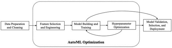
Figure 1.
Workflow of automatic machine learning.
AutoGluon, as an outstanding representative of the AutoML framework, has demonstrated its excellent prediction efficacy in several disciplines. In this study, AutoGluon is applied for the first time to the problem of structural crack propagation prediction in marine engineering to explore its potential application in this field. AutoGluon was chosen due to its advanced performance in automated feature engineering, model selection, and hyper-parameter optimization. The framework supports diverse machine learning models, including decision trees, random forests, gradient boosters, and neural networks, and is capable of automatically searching for optimal model architectures and parameter settings. AutoGluon achieves remarkable results thanks to its key technological strategies of model integration and multi-level stacking. The key technologies of AutoGluon are mainly the following three [31]:
(1) Stacking. This technique trains several different types of models on the same dataset, including, but not limited to, K-nearest neighbors (KNN), decision trees, and neural networks. The predicted outputs of these base models are combined into a single linear model, and the outputs of each model are weighted and summed through an ensemble learning technique, and a final prediction is generated.
(2) K-fold cross-bagging technique. As a form of ensemble learning, bagging reduces variance by constructing multiple models and averaging their predictions. These models may be based on different initial conditions or subsets of data. K-fold cross-bagging inherits the core idea of K-fold cross validation, i.e., the dataset is divided into K subsets, each of which is rotated as the validation set and the rest as the training set.
(3) Multi-level stacking technique. By integrating the predictions of multiple base models, the stacking method is applied again to form a higher-level model collection, and finally, the predictions are output via a linear model, the process is shown in Figure 2. In order to control overfitting, this technique is often used in combination with K-fold cross-bagging.
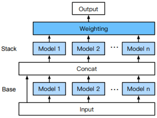
Figure 2.
AutoGluon’s multi-layer stacking strategy.
AutoGluon is suitable for all kinds of machine learning users due to its simplicity and efficiency and is able to realize model construction and automatic parameter tuning through minimal code [32], e.g., the prediction model in this paper has less than 20 lines of code. In view of this, AutoGluon is used as a research tool for crack propagation prediction in this study, as shown in the flow chart in Figure 3.
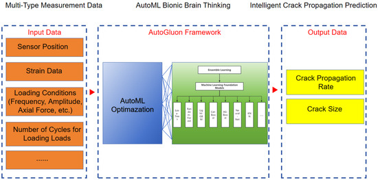
Figure 3.
Automatic machine learning based crack propagation prediction process.
2.2. Constructing Datasets Based on Fatigue Experiments
The literature [33] shows that structural strain measurements can accurately predict crack propagation. A study by Liang [21] further revealed the relationship between displacement field and fatigue crack propagation characteristics. Based on this, in this study, data such as the number of load cycles, strain, and crack dimension are collected through fatigue experiments on large-scale T-joints to form a dataset for AutoML. In this process, the input and output data mainly include the following:
- (1)
- Input data:
- Strain data.
- Cycle count.
- Loading conditions.
- Sensor position.
- (2)
- Output data:
- Crack propagation length or propagation rate.
The actual input data will be customized according to the experimental design, model selection, and application requirements, and the output data will be optimized for prediction purposes and user needs. The following section describes the specific methodology used to construct the dataset for this study.
2.2.1. Fatigue Experiment Materials
In this study, fatigue experiments were carried out for Q235B steel T-pipe joints, and specimens were manufactured by the shipyard of China Shipbuilding Group Co. The weld quality of the specimens was officially verified by the China Classification Society (CCS). As shown in Figure 4 and Table 1, the geometrical dimensions and key parameters of the experimental materials are listed, and the chemical composition and mechanical property data are displayed in Table 2 and Table 3, respectively. The T-joint members are welded by the chord and the brace, and the welding process follows the standard of the American Welding Society (AWS, 2008) [34]; the physical figure is shown in Figure 5. By comparing the experimental data from the literature [35,36], the specimens designed in this study are expanded in size by a factor of 1.6 to 2.7, respectively. This expansion helps to exclude boundary effects, i.e., the potential interference of the loading equipment on the experimental results.
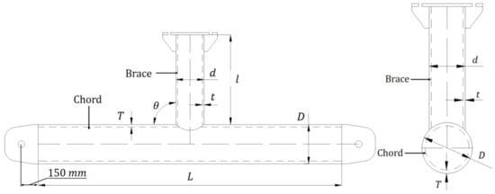
Figure 4.
Geometry and parameter definition of T-pipe joint specimen.

Table 1.
Geometric dimensions and parameters of T-joint specimens.
Table 2.
Chemical composition of specimen materials.
Table 3.
Main mechanical property parameters of specimen materials.
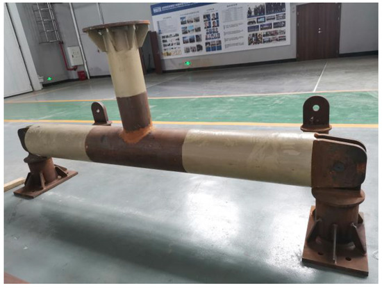
Figure 5.
Physical drawing of T-joint specimen.
2.2.2. Experimental Plan
In marine platform structures, T-joints are often exposed to complex multi-axial loading effects, of which axial loading is often the main form of loading [37]. Based on the above, this study focuses on such T-joints under axial tension, and the test setup together with the support frame is shown in Figure 6.
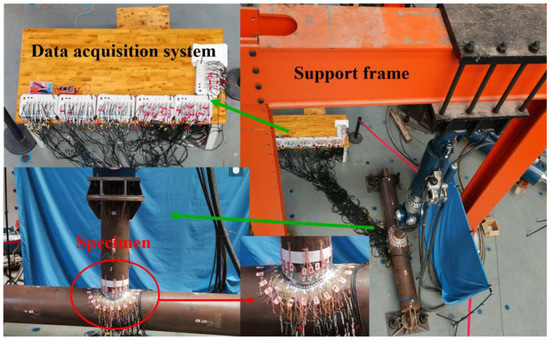
Figure 6.
Overall view of the T-joint experimental loading device.
The experiment was conducted at the Structural Engineering Laboratory. The experimental setup consists of an actuator (electro-hydraulic servo loading system), reaction frame, and anchoring screws. Each end of the specimen’s chord is equipped with side eye plates, which are connected to the central eye plate at the top of the pedestal via pin. The left and right pedestals are secured by two anchoring screws at their bottoms. The top of the brace is connected to the actuator via a flange, and the actuator is vertically fixed on the reaction frame to apply axial load to the brace. The actuator used in this experiment is a high-tonnage electro-hydraulic servo loading system manufactured by Servotest Testing Systems Ltd., Egham Surrey, UK, with the following main technical parameters: Test force: ±500 kN; Test frequency range: 0~20 Hz; Maximum test speed: 0.36 m/s; Actuator stroke: ±250 mm.
In order to ensure the effectiveness of the actuator load output, the maximum value of the fatigue load should not be less than 50% of the actuator loading capacity. In addition, according to the Steel Structure Design Standard (GB 50017-2017) [38], for T-tube joints subjected to axial tensile load at the end of the brace, the tensile load capacity should not exceed the calculated value of Equation (1).
where Ψd = 0.069 + 0.93β, β = 0.698, D = 351 mm, t = 14 mm, θ = 90°, Ψn = 1 (both sides of the chord are tensile), and f is the tensile strength of the chord material, which is taken to be 490.3 MPa.
In this experiment, a sinusoidal waveform was used for fatigue loading, with a set peak value of 300 kN, a valley value of 20 kN, an amplitude of 280 kN, a load ratio of 0.067, and a loading frequency of 0.6 Hz. The specific parameters are shown in Table 4, and the fatigue loading is shown in Figure 7.
Table 4.
Loading scheme for fatigue experiment.
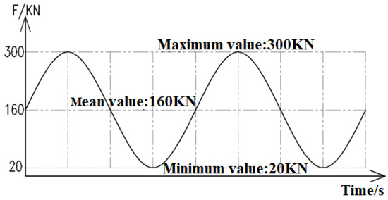
Figure 7.
Schematic fatigue load.
2.2.3. Dataset for Crack Measurement
In previous studies [11,12,35,36], high-speed/high-definition video cameras have been widely used to capture crack propagation in specimens. However, due to the tiny initial crack size and the possible corrosion on the surface of offshore structures, it is often difficult to obtain ideal results for observing surface cracks using this method. According to the research of Lv [39] and Shao [40], the ACPD technique can effectively monitor the crack propagation process in welded structures. Therefore, this study mainly adopts the ACPD method for quantitative measurement of crack propagation.
The ACPD method works as follows: the principle of skinning effect of high-frequency alternating current flowing through a ferromagnetic material is utilized to measure the depth of cracks on the surface of a metallic structure [40].
As shown in Figure 8, a current is passed through the surface of a metallic structure with a surface crack, ΔR is the reference probe spacing, ΔC is the spacing of the surface containing the crack (i.e., the working probe spacing), and in general, it can be made so that ΔC = ΔR. The potential falloff between ΔR is VR, the potential falloff between ΔC is VC, and d1 is the depth of the crack. The potential drop is proportional to the distance the current has traveled, then there is:
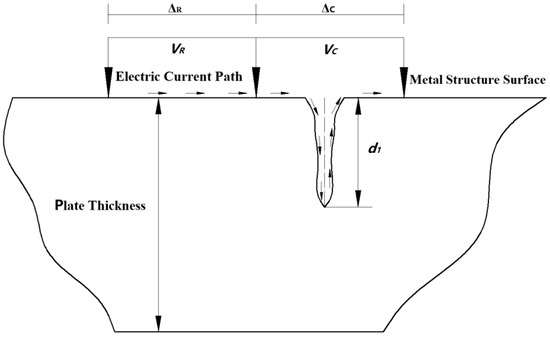
Figure 8.
Principle of ACPD method for measuring surface cracks.
Further, the crack depth can be derived as follows:
From Equation (4), it can be seen that the only external parameter related to the crack depth d1 is the reference probe distance ΔR, and ΔR is relatively easy to make accurate measurements in the experiment.
Based on the previous reasons, this experiment starts from the change of structural strain in the stage of crack initiation and proposes a method to precisely locate the position and moment of crack initiation by monitoring the strain response at each measurement point in the coherent loop direction of the pipe joint. Theoretically, if a crack does not appear at a point on the surface of the structure, the strain value at that point should remain stable under constant load. On the contrary, the appearance of cracks will cause significant fluctuations in the strain value. Accordingly, the monitoring of strain variations can be used to identify the exact location of crack initiation and to target the measurement of crack depth in that region. Currently, digital image correlation (DIC) techniques, fiber grating sensors, and conventional resistive strain gauges can be used for strain monitoring [41]. In this study, resistive strain gauges were selected for strain monitoring for the convenience of experimental operation.
From the literature [2], it can be seen that there exists a local peak value of hot spot stress amplitude between the chord saddle point and crown point of each specimen, and the extreme value is located from 90~180 degrees. Therefore, the extreme value of the hot spot stress amplitude and the neighboring areas are the key areas for strain monitoring. In addition, strain monitoring is also carried out in the vicinity of the local peak of each hot spot stress amplitude, as well as at the saddle point and crown point of the chord/brace. Taking specimen No. 3 as an example, its chord strain monitoring program and physical diagram are shown in Figure 9. The numbers from 0° to 355° in Figure 9 correspond to the positions of all strain gauge sensors, where the interval of the key monitoring area is 5° and the non-key monitoring area is 15°, so the density of the intervals of the lines in Figure 9a is not the same.
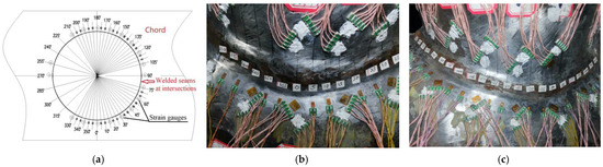
Figure 9.
String strain monitoring program and physical diagrams (Specimen #3): (a) Monitoring plan; (b) Physical diagram: 330° to 30°; (c) Physical diagram: 105° to 210°.
Cracks can be categorized into penetrating cracks, deeply embedded cracks, and surface cracks based on their geometrical properties. In the existing fatigue experimental studies, penetrating cracks are usually the main focus of research, and their length measurement methods have been thoroughly explored [42,43,44]. However, for marine structures, fatigue failures are often caused by the emergence and propagation of surface cracks. Therefore, fatigue experiments on tube nodes should not only observe the development of surface cracks but also make accurate quantitative measurements of their depths and lengths in order to fully understand the fatigue performance of pipe joints.
In this experiment, we used a handheld crack depth measuring instrument developed based on the ACPD principle to determine the crack depth. The specific appearance of the device is shown in Figure 10, and its main technical parameters are listed in Table 5.
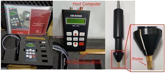
Figure 10.
Physical diagram of the crack depth gauge.
Table 5.
Main technical parameters of crack depth gauge.
In this study, the key data such as strain, number of load cycles, and crack depth are divided into the training set (80% of the data) and the test set (20% of the data). The training set is used for AutoGluon model construction and training, while the stability and generalization ability of the model is evaluated by the K-fold cross-bagging method. The hyper-parameter optimization of the model is done with the help of the Bayesian optimization technique embedded in AutoGluon. In order to verify the generalization performance of the model, crack depth data under different conditions are selected for testing.
2.2.4. Principle of Crack Propagation Rate Calculation
The fatigue crack propagation rate is the amount of fatigue crack propagation for one load cycle, and the crack propagation rate is closely related to the range of stress intensity factor at the crack tip. In general, the da/dN-ΔK curve can be divided into three regions: region I is the slow crack propagation region, region II is the stable crack propagation region, and region III is the unstable crack propagation region. The fatigue life of the structure basically depends on the crack propagation in region II. The relationship between da/dN and ΔK in this region can be expressed as the Paris equation [45]:
where a is the crack size, which is usually the crack depth or half width for surface cracks, and N is the number of fatigue loading cycles. The coefficients C and m are the fatigue crack propagation constants, which are obtained by the experiment. ΔK is the stress intensity factor range, which is expressed as:
where Y is the crack geometry correction factor and Δσ is the hot spot stress range.
The standard BS 7910 [46] expresses ΔK as primary and secondary stress components as follows:
where (YΔσ)P and (YΔσ)S are the initial stress range and secondary stress range components, respectively, considering the crack geometry correction factor Y.
Only the initial stress component is taken into account in the fatigue crack propagation calculations, which are formulated as follows:
where M is the expansion correction factor and fw is the crack surface correction factor, which are calculated as shown in Annex M of [46]. Mm, Mb, Mkm, and Mkb are the stress amplification factors, which are calculated as shown in Annexes M and B of [46]. Ktm and Ktb are the membrane stress and bending stress concentration factors, respectively, which are taken as the corresponding stress concentration factors of the T-pipe joints at the location of the cracks in the present calculations. Km is the stress amplification factor due to structural misalignment, which is calculated in Annex D of [46]. Δσm and Δσb are the membrane stress range and bending stress range, respectively.
Membrane stress and bending stress components can be obtained from hot spot stress calculations according to the literature [46]:
where Ω is the pipe joint curvature, which is a physical parameter describing the ratio of bending stress to membrane stress applied to the pipe joint and can be calculated according to the fitting formula given in the literature [46].
Due to space limitations, this paper only lists the bending degree calculation formula for the ratio of bending stress to total stress under axial load for the hot spot stress of the chord, as follows:
where α, β, γ, τ, θ are the specimen geometric parameters, which are defined as shown in Table 1.
Similarly, in the fatigue crack propagation calculation, if the fatigue hot spot stress range is Δσhs, the membrane stress range and bending stress range are as follows:
2.3. Evaluation Metrics for AutoML
When evaluating the prediction accuracy of a model, its performance metrics on the test set need to be calculated. For classification tasks, common metrics include accuracy, precision, recall, and F1-Score, while in regression tasks, metrics such as mean-square error (MSE), root mean square error (RMSE), mean absolute error (MAE), or coefficient of determination (R2 score) can be used. Given that the crack propagation prediction in this study is essentially a regression problem, and referring to the studies of Liang (2024) and Fang (2022), we mainly adopt the root mean square error (RMSE) as the evaluation criterion of the AutoML model, and supplement it with other metrics to fully demonstrate the prediction efficacy of the model when necessary.
Root mean square error (RMSE) is a statistical metric that measures the degree of deviation of the predicted value from the actual value. In this study, RMSE is mainly used to quantify the average deviation between the predicted data and the experimental data, which is calculated as follows [27]:
where m is the sample number, is the sample of the test set, and is the predicted outcome of the model.
3. Results and Discussion
The combination of strain monitoring and crack measurement techniques allows us to obtain the data needed to predict crack propagation. According to the fatigue cumulative damage theory, crack initiation on the structural surface is triggered by the continuous accumulation of fatigue damage, and the crack will continue to propagate under cyclic loading. Figure 11 shows a schematic diagram of the complete process of crack propagation for specimens 1 to 3. The crack propagation process in the figure refers to the location where the crack appears under the corresponding number of cycles. That is, the different arcs indicate the location and length of the crack under the number of cycles, as shown in Figure 11.
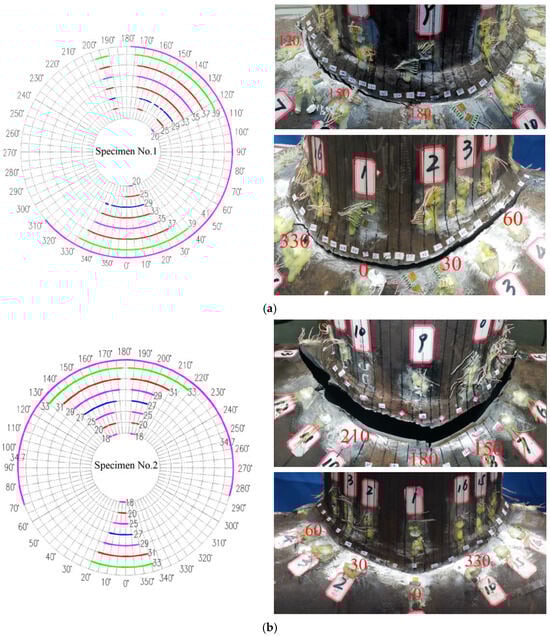
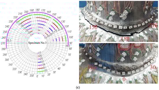
Figure 11.
Schematic diagram of the whole process of crack propagation: (a) Schematic diagram of crack propagation process and final state of specimen No. 1 (20~41 is the number of load cycles, unit: 10,000 times); (b) Schematic diagram of crack propagation process and final state of specimen No. 2 (18~34.7 is the number of load cycles, unit: 10,000 times); (c) Schematic diagram of crack propagation process and final state of specimen No. 3 (17~35.3 is the number of load cycles, unit: 10,000 times).
From Figure 11a, it can be seen that the crack propagation of specimen No. 1 mainly starts from the vicinity of 132.5 degrees and 7.5 degrees, and at 7.5 degrees, the cracks basically propagate uniformly left and right along the coherent line. From Figure 11b, it can be seen that the crack propagation of specimen No. 2 mainly starts near 5 degrees, 160 degrees, and 190 degrees, and the cracks at these three positions basically expand uniformly along the coherent line left and right. From Figure 11c, it can be seen that the crack extension process of specimen No. 3 is generally more similar to that of specimen No. 2. For specimen No. 3, the vicinity of 5 degrees, 140 degrees, 172.5 degrees, and 205 degrees are the main crack initiation points and the starting points of subsequent crack propagation.
Due to space limitations, only specimen No. 1 is described in detail in this paper. In Figure 11a, the crack propagation analysis of specimen No. 1 shows that two crack initiations were observed at 200,000 cycles (N = 200,000). As the number of cycles increased to 250,000 and 290,000, the number of cracks increased and showed interrupted lines with multiple cracks expanding simultaneously. By 330,000 cycles (N = 330,000), the multiple crack propagation terminated, and a single main crack was formed. After 390,000 cycles, crack penetrations occurred in the specimen at approximately 132.5 degrees and 7.5 degrees.
Taking specimen No. 3 as an example, Table 6 and Figure 12 record the strain changes and crack depth data during crack initiation and propagation. The data in Table 6 show that at the crack initiation point or its neighboring region, there is a tendency for the strain value to decrease with the increase in the number of load cycles. In the monitoring of this large-scale T-pipe joint fatigue experiment, we arranged strain gauges at 5-degree intervals in the critical region. According to experience, when the strain value decreases beyond a certain threshold (usually 3% or more), it indicates that crack initiation may have occurred at the monitoring point or in the neighboring area, and more detailed measurements are required at this time. For example, at the monitoring location of 170° in this study, the first cracks appeared at 172° based on the change in strain.
Table 6.
Strain and crack depth monitoring results at crack initiation stage.
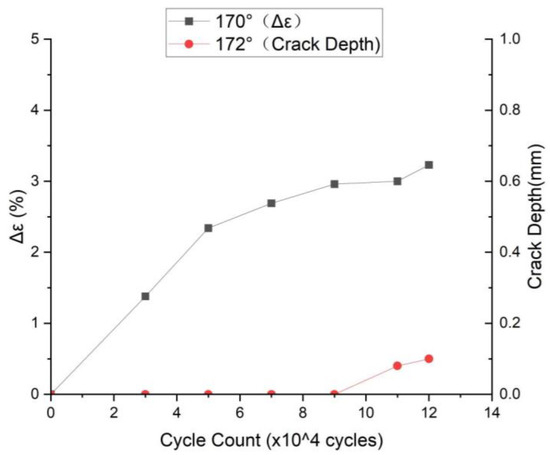
Figure 12.
Strain rate of change at the monitoring point and depth of crack initiation.
In this paper, taking specimen No. 3 in this experiment as an example, the crack depth values of 0.4 mm to 0.55 mm can be measured at 172.5 degrees by using the ACPD crack depth gauge when a strain drop of 3% (number of cycles N = 110,000) and 3.23% (N = 120,000), respectively, is observed at the 170-degree position. It is important to note, however, that the ACPD method has been shown to be effective in measuring metal crack depth, and especially in the measurement of shallow cracks, where there are limitations in accuracy and sensitivity [47]. Therefore, when the strain change rate is less than 3%, it does not mean that there is no crack initiation. However, based on experience and existing crack size measurement techniques, when the rate of strain change is close to 3%, it may indicate initial crack formation. It can be seen that the strain monitoring method can provide a quick and accurate prediction of the crack initiation point or region, which helps to pinpoint and capture the moment of crack initiation in time and is a recommended monitoring tool.
3.1. Prediction and Analysis of Crack Propagation Rate Based on AutoML
Based on the experimental measurements, we were able to directly derive curves describing the relationship between the crack depth and the number of load cycles N, as well as the relationship between the crack width (half-width) c and the number of load cycles N. These curves provide us with a quantitative description of the crack propagation behavior.
Crack propagation data for three specimens in a specific angular range were selected for this study: the region from 40° to 330° for specimen No. 1, the region from 130° to 170° for specimen No. 2, and the region from 150° to 190° for specimen No. 3. Based on these data, a-N curves were plotted as well as c-N, and the graphs of these curves are shown in Figure 13. In particular, it is noted that Figure 13 takes the data at crack depths up to approximately 1 mm as the starting point for the analysis and does not take into account the data at the stage of smaller crack depths in an attempt to reduce the element of uncertainty in the data.
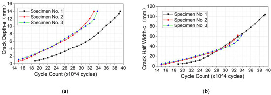
Figure 13.
Curve of crack size vs. number of load cycles: (a) a~N curve; (b) c~N curve.
As can be observed from Figure 13, the a-N curves and c-N curves of each specimen exhibit similar general trends. Specifically, specimen No. 1 recorded the highest number of maximum load cycles and the corresponding maximum crack half-width for each specimen when the crack depth fully penetrated the 14 mm wall thickness. In contrast, the number of load cycles corresponding to crack depth penetration through the wall thickness for specimens No. 2 and No. 3 were similar to each other, and their final crack half-widths also showed a high degree of consistency. These observations suggest that the load cycling capacity and crack size of different specimens show a certain regularity when the crack extends to a certain critical depth.
The crack propagation rate at each point on the curve can be obtained from the a~N and c~N curves. In this paper, the incremental polynomial method is used to process the a~N data of the test to determine the fatigue crack depth expansion rate da/dN and the fitted value of crack depth ai. A quadratic polynomial in the form of Equation (16) is used to fit the derivatives for any data points i and n before and after the experiment, for a total of 2n + 1 consecutive data points, and n is taken as 3 in this paper.
where , , and . b0, b1, and b2 are regression parameters determined by the least squares method over the interval. The fitted values ai are the fitted crack depths corresponding to the number of cycles Ni. The crack depth propagation rate at Ni is:
The fitted crack depth ai at Ni is then used to calculate the stress intensity factor range (ΔK)ai value corresponding to the (da/dN)ai value, and the crack propagation rate da/dN versus ΔK curve can be obtained.
Furthermore, taking logarithms on both sides of Equation (16), we have:
It can be seen that lg(da/dN) is linearly related to lg(ΔK), and C and m can be obtained by linear regression of the data using the least squares method. The crack width propagation rate (dc/dN) versus ΔK at each point on the c~N curve can also be calculated and fitted using the method described above.
The training set was first constructed with the da/dN data of specimen No. 2 and specimen No. 3, and the da/dN of specimen No. 1 was predicted. Then the data of specimen No. 1 and specimen No. 3 were set as the training set, and the prediction of specimen No. 2 was made. The prediction results are shown in Figure 14. The AutoML model prediction results of specimen No. 1 are compared and analyzed with the actual experimental data, and the results show a high consistency between them. The overall trend of the prediction results of specimen No. 2 is basically consistent with the experimental results, except that there are some data points with differences, which is due to the relatively small amount of training data. On the whole, the crack propagation process can be divided into two stages, and the crack propagation rate and the stress intensity factor magnitude (ΔK) in each stage show a significant linear correlation. The first stage mainly corresponds to crack initiation and initial propagation, when the magnitude of the stress intensity factor is low and the crack propagation rate is correspondingly slow. When the magnitude of the stress intensity factor reaches a certain critical value, the crack propagation enters the second stage, at which the magnitude of the stress intensity factor increases rapidly, and the crack propagation rate is accelerated accordingly.
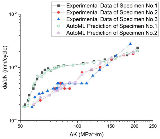
Figure 14.
Crack propagation rate vs. stress intensity factor for all specimens.
In the AutoGluon framework, the regression evaluation metrics can be calculated by writing the corresponding code; the specific code and calculation process are shown in Figure 15, and the results of the evaluation metrics are shown in Table 7. Given that these metrics are essentially loss functions, the evaluation criterion is that the smaller the value, the better the performance of the model. According to the data in Table 7, the values of the three regression evaluation metrics used in this study are quite low, ranging from 5.46 × 10⁻⁴ to 2.99 × 10⁻⁷, which indicates that the results of AutoML in predicting the rate of node crack propagation of large-scale T-joints are satisfactory.
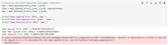
Figure 15.
Results of evaluation metrics for predicting crack propagation rate in AutoGluon.
Table 7.
Evaluation metric results for crack propagation stage.
In the previous section, a preliminary evaluation of the performance of the AutoML model has been made by comparing the results of the various regression evaluation metrics. Further, if we need to obtain the accuracy ranking similar to that in the classification problem, we can refer to the score_val column in the leaderboard, which demonstrates the value of the loss function. In AutoGluon’s AutoML framework, the leaderboard serves as a comprehensive evaluation tool that presents the performance of different models on specific datasets by visual means, which facilitates researchers to compare, select, and optimize the system. This function not only enhances the transparency and repeatability of the model selection process but also provides a standardized evaluation benchmark for the machine learning field, thus improving the efficiency and accuracy of the automated design and evaluation process.
Therefore, the “predictor.leaderboard()” code can be used to show the performance of different machine learning models on the crack propagation prediction task, and the specific results are shown in Figure 16. In this evaluation system, the closer the value is to 0 (i.e., the smaller the absolute value of the loss function value is), it means that the model performs better on the validation set. For regression problems, such as crack propagation prediction, score_val usually represents the negative root mean square error (RMSE) or other similar loss function values. The results of the score_val columns shown in Figure 16 reveal that on the validation set, the AutoGluon ensemble learning approach (WeightedEnsemble) exhibits better performance compared to single machine learning models such as random forests and neural networks, suggesting that AutoGluon has a stronger predictive capability in such prediction tasks.
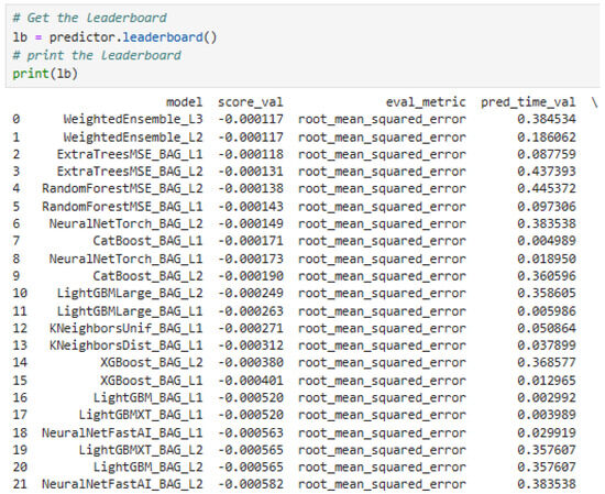
Figure 16.
Leaderboard results for predicting crack propagation rate.
3.2. Prediction and Analysis of Crack Geometric Dimensions Based on AutoML
According to the previous analysis, the strain rate of change () at the monitoring points is closely related to the state of crack initiation and propagation and can be used as a key characteristic index for predicting the size of crack propagation. In this study, taking specimen No. 3 as an example, the training and testing dataset of the AutoML model was constructed based on the strain change rate of each monitoring point and its measured crack depth value under a different number of load cycles. The feature values mainly include the location of the monitoring point, the number of load cycles, and the corresponding strain values, while the regression prediction targets the crack depth in and around the monitoring point. Figure 17 shows the relationship between crack depth and strain change rate for some of the monitoring points of specimen No. 3, and, due to space limitations, only the data of the monitoring points from 170° to 210° in the core area of crack propagation are shown.
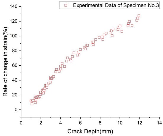
Figure 17.
Crack depth versus strain change rate at different monitoring points (Specimen No. 3).
Figure 18 illustrates a schematic of the depth of crack propagation for specimen No. 3 at position 172° as the number of cycles of different loads increases. Experimental values and AutoGluon’s predicted values are included in the figure.
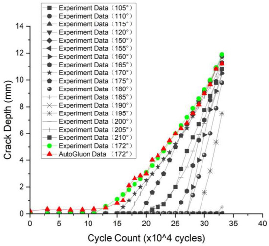
Figure 18.
Relationship between crack propagation depth and different numbers of load cycles (Specimen No. 3).
Figure 18 shows that, in general, the crack depth trends predicted by AutoML are generally consistent with the fatigue experimental measurements. However, there is a certain deviation between the AutoML predicted values and the experimental values at the crack initiation stage of specimen No. 3, i.e., when the number of load cycles is in the interval of 0 to 110,000 cycles. This paper analyzes that this deviation may be caused by the following two factors: First, the amount of experimental data is insufficient, resulting in the training model not being able to fully capture the real process of crack propagation. Second, in the fatigue crack sizing assessment of metallic structures, the alternating current potential drop (ACPD) technique, although excellent in detecting deep cracks, may face challenges of accuracy and sensitivity in identifying shallow cracks. Although the ACPD technique may not be able to detect the phenomenon of tiny crack initiation at strain change rates below 3% (i.e., crack sizes less than 0.5 mm), based on experience and available experimental data on fatigue crack propagation, the initial formation of cracks can be observed when the strain change rate is near or above this threshold. This extrapolation based on experience and the scientific method provides a more rigorous and logical way to identify and monitor cracks at an early stage.
In agreement with the previously described methodology, the evaluation metrics obtained from AutoGluon calculations were used to measure the model performance in this study, and the detailed evaluation results are shown in Table 8 and Figure 19. The data in Table 8 show that the regression evaluation metrics used to predict the crack depths have relatively low values, which are distributed in the range from 0.11 to 0.33. Although the values of these metrics are higher than the evaluation metrics for the crack propagation rate of large-scale T-joints, considering that crack depths are usually small in size during the initiation stage and that there may be some accuracy limitations in the ACPD measurement technique, this study still concludes that the use of AutoML for predicting the crack propagation depths in metal fatigue experiments of large-scale T-joints is reliable.
Table 8.
Results of evaluation metrics for crack depth prediction.
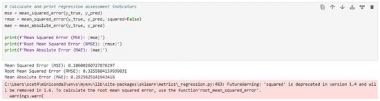
Figure 19.
Results of regression evaluation metrics for crack depth prediction in AutoGluon.
In the process of using AutoML techniques for crack depth prediction, this study utilizes the leaderboard function of AutoGluon to compare and analyze the performance of the integrated model with that of a single machine learning model. The leaderboard not only demonstrates the performance metrics of the final integrated model, but also lists in detail the performance of the individual base models contributing to the integration process performance. Figure 20 shows the leaderboard results for AutoML crack propagation prediction, while Figure 21 further presents the loss function values of each model when predicting crack depth, thus providing an intuitive reference for evaluating the prediction effectiveness of different models.
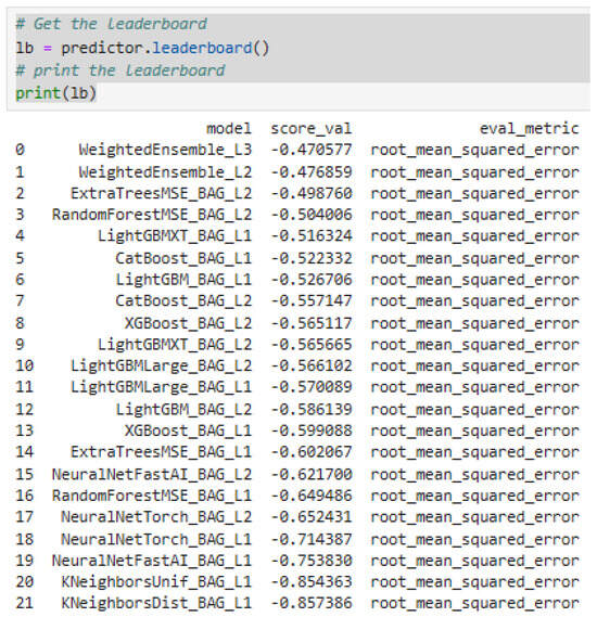
Figure 20.
Leaderboard results for crack depth prediction.
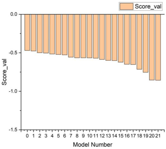
Figure 21.
Loss function values for crack depth prediction.
In the results shown in Figure 20, WeightedEnsemble usually refers to the integrated model, while RandomForest, LightGBMXT, KNeighbors, etc. represent the base models that make up the integrated model. The figure clearly shows the score_val performance metrics of each model on the validation set. Further observation of Figure 21 shows that the score_val of the integrated model is generally better than that of the single base model. The WeightedEnsemble_L3 model after 3-fold cross-bagging, for example, significantly exceeds the performance of the other foundation models. For example, in crack size prediction, WeightedEnsemble_L3’s loss function (−0.470577) has a 5.65% accuracy improvement over the foundation model ExtraTreesMSE_BAG_L2 (−0.49876), which has the best prediction results. This result indicates that AutoGluon is able to achieve more accurate prediction results by integrating multiple models, thus significantly improving the accuracy of crack depth prediction.
4. Conclusions
This study proposes a metal fatigue crack propagation prediction method based on AutoML. By comparing its performance with a single machine learning model, an efficient ensemble learning prediction model is established, and its accuracy is verified by experimental data of a large-scale T-joint. The conclusions obtained are as follows:
(1) AutoGluon was able to significantly improve the accuracy of crack propagation prediction compared to a single machine learning model through ensemble learning. In the large-scale T-pipe joint crack size prediction, the integrated learning is 5.65% more accurate than the foundation model with the best prediction results. Meanwhile, the appropriate amount of stacking and cross-bagging is essential to enhance the predictive performance of the model. However, the use of these methods needs to be balanced between improving performance and controlling computational costs.
(2) As the number of load cycles increases, the strain at the crack initiation point or its neighboring region usually shows a decreasing trend, and when the strain decreases by more than 3% compared to the initial value, crack initiation may occur in the vicinity of the monitoring point, and then targeted measurements are required. Compared to the accuracy of traditional crack measurement techniques, the prediction method using AutoML is able to identify the initial crack initiation point more efficiently, thus providing a significant advantage in the early stages of crack propagation.
(3) The AutoML-based crack propagation rate prediction method proposed in this study is able to accurately identify the two main stages of the crack propagation process and reveals a significant linear correlation between the da/dN and the magnitude of the ΔK within each stage. In the initial stage, the cracks mainly experience initiation and slow propagation when ΔK is relatively low, resulting in a correspondingly slow da/dN. With the increase of ΔK reaching a critical value, the crack propagation enters into an accelerated phase, where ΔK increases rapidly and da/dN accelerates significantly.
(4) Although the prediction results at the initial stage of crack depth prediction have some deviation from the experimental values, the prediction results are basically consistent with the experimental values at other propagation stages. The main reason for the initial prediction deviation may be related to the insufficient amount of crack depth data measured during the crack initiation stage. This may be a limitation of the ACPD technique in terms of detection accuracy. Therefore, in order to improve the measurement accuracy at the crack initiation stage, it is necessary to develop higher-precision crack measurement methods.
In the future work, attention will be focused on the following directions: first, the development of crack measurement techniques with high accuracy. Second, to study the fatigue crack propagation of large-scale T-pipe joints in corrosion environments, so as to construct more accurate prediction models.
Author Contributions
Conceptualization, P.L., Y.Y. and C.C.; methodology, P.L. and Y.Y.; software, P.L.; validation, P.L. and Y.Y.; formal analysis, P.L.; investigation, P.L., Y.Y. and C.C.; resources, C.C.; data curation, P.L. and Y.Y.; writing—original draft preparation, P.L. and Y.Y.; writing—review and editing, P.L., Y.Y. and C.C.; visualization, P.L. and Y.Y.; supervision, C.C.; project administration, C.C.; funding acquisition, C.C. All authors have read and agreed to the published version of the manuscript.
Funding
This research was funded by the Key-Area Research and Development Program of Guangdong Province, China (Grant No. 2021B0707040002), the National Natural Science Foundation of China (Grant No. 51979111), and the project of New Energy Joint Laboratory of China Southern Power Grid Corporation (GDXNY2022KF03).
Institutional Review Board Statement
Not applicable.
Informed Consent Statement
Not applicable.
Data Availability Statement
The original contributions presented in the study are included in the article, further inquiries can be directed to the corresponding authors.
Conflicts of Interest
The authors declare no conflicts of interest.
References
- DNV GL. Fatigue Assessment of Ship Structures. In DNV GL Class Guideline DNVGL-CG-0129; DNV GL: Oslo, Norway, 2018; pp. 48–52. [Google Scholar]
- Chen, C.-H.; Yang, Y.-F.; Li, P.; Jiao, J.-L. Review of Corrosion Damage and Corrosion Fatigue Evaluation Methods for Marine Structures. J. Ship Mech. 2023, 27, 1413–1429. [Google Scholar] [CrossRef]
- Adilah, A.; Iijima, K. A Spectral Approach for Efficient Fatigue Damage Evaluation of Floating Support Structure for Offshore Wind Turbine Taking Account of Aerodynamic Coupling Effects. J. Mar. Sci. Technol. 2021, 27, 408–421. [Google Scholar] [CrossRef]
- Song, Y.; Xu, Z.; Zhang, J.; Li, G.; Yang, P. Experimental Study of Low-Cycle Fatigue Crack Propagation in Hull Stiffened Plates with Symmetric and Asymmetric Cracks. Ocean Eng. 2024, 299, 117303. [Google Scholar] [CrossRef]
- Shi, X.H.; Zhang, J.; Soares, C.G. Numerical Assessment of Experiments on the Residual Ultimate Strength of Stiffened Plates with A Crack. Ocean Eng. 2019, 171, 443–457. [Google Scholar] [CrossRef]
- Hu, K.; Yang, P.; Xia, T.; Song, Y.; Chen, B. Numerical Investigation on the Residual Ultimate Strength of Cracked Stiffened Plates Under Extreme Cyclic Loads. Ocean Eng. 2022, 244, 110426. [Google Scholar] [CrossRef]
- Yu, C.-L.; Chen, Y.-T.; Yang, S.; Liu, Y.; Lu, G.C. Ultimate Strength Characteristic and Assessment of Cracked Stiffened Panel under Uniaxial Compression. Ocean Eng. 2018, 152, 6–16. [Google Scholar] [CrossRef]
- Dong, Z. Fatigue Crack Propagation at Typical Details of Hull under Low Temperature Environment; Harbin Engineering University: Harbin, China, 2023; pp. 69–74. [Google Scholar]
- Chen, Z.; Liu, Y.; Qian, H.; Wang, P.; Liu, Y. Effect of Repair Welding on the Fatigue Behavior of AA6082-T6 T-Joints in Marine Structures Based on FFS and Experiments. Ocean Eng. 2023, 281, 114676. [Google Scholar] [CrossRef]
- Tu, W.; Yue, J.; Xie, H.; Tang, W. Fatigue Crack Propagation Behavior of High-Strength Steel under Variable Amplitude Loading. Eng. Fract. Mech. 2021, 247, 107642. [Google Scholar] [CrossRef]
- Zhang, Z. Research on Fatigue Behaviour of Stainless Steel Welded Tubular T-Joints; Hefei University of Technology: Hefei, China, 2021; pp. 42–64. [Google Scholar]
- Yang, Z. Fatigue Behavior of CHS T-Joints with High Strength Steel Q460C under Cyclic In-Plane Bending; Chongqing University: Chongqing, China, 2018; pp. 11–38. [Google Scholar]
- Dou, R.; Li, H. Experimental Study on Static Force and Fatigue of Large-Scale T-welded Pipe Nodes on Offshore Platforms. China Offshore Platform. 1994, Z1, 232–239. [Google Scholar]
- Ahmadi, H.; Ghaffari, A. Probabilistic analysis of stress intensity factor (SIF) and degree of bending (DoB) in axially loaded tubular K-joints of offshore structures. Lat. Am. J. Solids Struct. 2015, 12, 2025–2044. [Google Scholar] [CrossRef]
- Ahmadi, H.; Mousavi Nezhad Benam, M.A. Probabilistic analysis of stress concentration factors in unstiffened gap tubular KT-joints of jacket structures under the out-of-plane bending moment loads. Adv. Struct. Eng. 2017, 20, 595–615. [Google Scholar] [CrossRef]
- Li, Z.; Han, F. The Peridynamics-Based Finite Element Method (PeriFEM) with Adaptive Continuous/Discrete Element Implementation for Fracture Simulation. Eng. Anal. Bound. Elem. 2023, 146, 56–65. [Google Scholar] [CrossRef]
- Ilie, P.; Ince, A. Three-Dimensional Fatigue Crack Growth Simulation and Fatigue Life Assessment Based on Finite Element Analysis. Fatigue Fract. Eng. Mater. Struct. 2022, 45, 3251–3266. [Google Scholar] [CrossRef]
- Bordas, S.-P.-A.; Rabczuk, T.; Hung, N.-X.; Nguyen, V.P.; Natarajan, S.; Bog, T.; Hiep, N.V. Strain Smoothing in FEM and XFEM. Comput. Struct. 2010, 88, 1419–1443. [Google Scholar] [CrossRef]
- Xie, G.; Zhao, C.; Li, H.; Liu, J.; Zhong, Y.; Du, W.; Lv, J.; Wu, C. An Adaptive Extended Finite Element Based Crack Propagation Analysis Method. Mech. Technol. 2024, 30, 74–82. [Google Scholar] [CrossRef]
- Lv, W.; Ding, B.; Zhang, K.; Qin, T. High-Cycle Fatigue Crack Growth in T-Shaped Tubular Joints Based on Extended Finite Element Method. Buildings 2023, 13, 2722. [Google Scholar] [CrossRef]
- Xie, G.; Jia, H.; Li, H.; Zhong, Y.; Du, W.; Dong, Y.; Wang, L.; Lv, J. A Life Prediction Method of Mechanical Structures Based on the Phase Field Method and Neural Network. Appl. Math. Model. 2023, 119, 782–802. [Google Scholar] [CrossRef]
- Bashiri, A.-H.; Alshoaibi, A.-M. Adaptive finite element prediction of fatigue life and crack path in 2D structural components. Metals 2020, 10, 1316. [Google Scholar] [CrossRef]
- Liang, J.; Yu, Y.; Hu, W. Prediction of Fatigue Crack Growth in Metal Materials via Spatiotemporal Neural Network. J. Shanghai Jiao Tong Univ. (Sci.) 2024, 1–17. [Google Scholar] [CrossRef]
- Strohmann, T.; Starostin, P.-D.; Breitbarth, E.; Requena, G. Automatic Detection of Fatigue Crack Paths Using Digital Image Correlation and Convolutional Neural Networks. Fatigue Fract. Eng. Mater. Struct. 2021, 44, 1336–1348. [Google Scholar] [CrossRef]
- Feng, S.-Z.; Han, X.; Li, Z.; Incecik, A. Ensemble Learning for Remaining Fatigue Life Prediction of Structures with Stochastic Parameters: A Data-Driven Approach. Appl. Math. Model. 2022, 101, 420–431. [Google Scholar] [CrossRef]
- Wang, B.; Xie, L.; Song, J.; Zhao, B.; Li, C.; Zhao, Z. Curved Fatigue Crack Growth Prediction under Variable Amplitude Loading by Artificial Neural Network. Int. J. Fatigue 2021, 142, 105886. [Google Scholar] [CrossRef]
- Do, D.; Lee, J.; Nguyen-Xuan, H. Fast Evaluation of Crack Growth Path Using Time Series Forecasting. Eng. Fract. Mech. 2019, 218, 106567. [Google Scholar] [CrossRef]
- Dung, C.-V.; Sekiya, H.; Hirano, S.; Okatani, T.; Miki, C. A Vision-Based Method for Crack Detection in Gusset Plate Welded Joints of Steel Bridges Using Deep Convolutional Neural Networks. Autom. Constr. 2019, 102, 217–229. [Google Scholar] [CrossRef]
- Fang, X.; Liu, G.; Wang, H.; Xie, Y.; Tian, X.; Leng, D.; Mu, W.; Ma, P.; Li, G. Fatigue Crack Growth Prediction Method Based on Machine Learning Model Correction. Ocean Eng. 2022, 266, 112996. [Google Scholar] [CrossRef]
- Waring, J.; Lindvall, C.; Umeton, R. Automated Machine Learning: Review of the State-of-the-Art and Opportunities for Healthcare. Artif. Intell. Med. 2020, 104, 101822. [Google Scholar] [CrossRef]
- Erickson, N.; Mueller, J.; Shirkov, A.; Zhang, H.; Larroy, P.; Li, M.; Smola, A. Autogluon-Tabular: Robust and Accurate AutoML for Structured Data. arXiv 2020, arXiv:2003.06505. [Google Scholar]
- Li, P.; Chen, C.-H. Damage Identification of Mooring System for Offshore Structure with Automated Machine Learning. In Proceedings of the International Ocean and Polar Engineering Conference, Shanghai, China, 6–10 June 2022. ISOPE-I-22-221. [Google Scholar]
- Katsikeros, C.-E.; Labeas, G.-N. Development and Validation of a Strain-Based Structural Health Monitoring System. Mech. Syst. Signal Proc. 2009, 23, 372–383. [Google Scholar] [CrossRef]
- American Welding Society (AWS). Structural Welding Code-Steel; American Welding Society: Miami, FL, USA, 2008; pp. 163–186. [Google Scholar]
- Zhang, Z. Study on High Cycle Fatigue Behavior of T-shaped Circular Steel Pipe Joints under Marine and Atmospheric Environment; China University of Mining and Technology: Xuzhou, China, 2019; pp. 49–63. [Google Scholar]
- Zhang, S. Study on Static and Dynamic Mechanical Properties of Corroded CHS T-Joints; China University of Mining and Technology: Xuzhou, China, 2021; pp. 32–86. [Google Scholar]
- Gan, J. Research on Key Technologies for Muliti-Purpose Jack-Up Platform Structure Design; Wuhan University of Technology: Wuhan, China, 2012; pp. 104–108. [Google Scholar]
- GB 50017-2017; Code for Design of Steel Structures. China Standards Press: Beijing, China, 2017; pp. 126–142.
- Lv, Y.; Shao, Y. Measurement of the Development of Fatigue Crack in Tubular Joints Using ACPD Technique. Ind. Constr. 2006, 442–444. Available online: https://kns.cnki.net/kcms2/article/abstract?v=6TwuVQQ8bf8VGrvvZYF_qFmDtiuxbDA5dJNWWLMwYQKCWV_e_oDyqb1WxJ-RJ4KW9LDIIpHBIxRFEiXQKYorzeocF0arOWr4ipVih9QIoFRivD0iUJ38iCg8wMn27SpCQA0G70g0MfmjsCZnOAcPMsBtHTH3WXtN9PoHe9qr6ktxhnqlCuem3q2bly2vqurQeFS_tWSv2PvGJ6RsHtuvLg==&uniplatform=NZKPT&language=CHS (accessed on 27 July 2024).
- Shao, Y. Measuring Crack Propagation of Welded Tubular Joints by Using ACPD Technique. Struct. Res. 2010. Available online: https://kns.cnki.net/kcms2/article/abstract?v=6TwuVQQ8bf9YxlfSoHhlcgoNt_Fn3BvnC1l-3d6SbZKj25jeGuaxNU3N7Z664P1qTAaGphi2LipNGZ_X1YB6JI78rx_KwH6lHeU5pWTAUUfcm5PD8c4nky_Pe6mx7c-ZR-vuT11RkzzguhPJtm4IpIj_3K0Cimgz4tWRn7UdpzyLCXv6OqFF3qtmyvNBl-ZRDn4M4ng1JNk=&uniplatform=NZKPT&language=CHS (accessed on 27 July 2024).
- Chandra, V.; Chakraborty, P. Automated Crack Extension Measurement Method for Fracture and Fatigue Analysis Using Digital Image Correlation. Eng. Fract. Mech. 2024, 305, 110182. [Google Scholar] [CrossRef]
- Wang, Y.-T.; Feng, G.-Q.; Li, C.F.; Lin, Y. Crack Propagation Rate Tests of Marine Steel Q235. J. Harbin Eng. Univ. 2015, 36, 1302–1306. [Google Scholar]
- Chen, Y.-Q. Experimental Research on Crack Length Measurement Method of Three Point Bending Specimen; Dalian University of Technology: Dalian, China, 2016; pp. 33–47. [Google Scholar]
- Huang, X.-W.; Shan, X.-F.; Gao, H.-L.; Chen, W. Fatigue Crack Length Measurement Method Based on Edge Detection and DIC. Acta Armamentarii 2022, 43, 940–951. [Google Scholar]
- Yin, Z. Structural Fatigue and Fracture, 1st ed.; Northwestern Polytechnical University Press: Xi’an, China, 2012; pp. 154–196. [Google Scholar]
- BS 7910; Guide to Methods for Assessing the Acceptability of Flaws in Metallic Structures. British Standard Institution: London, UK, 2013; pp. 134–150.
- Li, Y.; Gan, F.; Wan, Z.; Liao, J.; Li, W. Novel Method for Sizing Metallic Bottom Crack Depth Using Multi-Frequency Alternating Current Potential Drop Technique. Meas. Sci. Rev. 2015, 15, 268. [Google Scholar] [CrossRef]


Disclaimer/Publisher’s Note: The statements, opinions and data contained in all publications are solely those of the individual author(s) and contributor(s) and not of MDPI and/or the editor(s). MDPI and/or the editor(s) disclaim responsibility for any injury to people or property resulting from any ideas, methods, instructions or products referred to in the content. |
© 2024 by the authors. Licensee MDPI, Basel, Switzerland. This article is an open access article distributed under the terms and conditions of the Creative Commons Attribution (CC BY) license (https://creativecommons.org/licenses/by/4.0/).