Predictions of the Effect of Non-Homogeneous Ocean Bubbles on Sound Propagation

Abstract

In the ocean, bubbles rarely appear alone and are often not evenly distributed, which makes it complicated to predict the effect of ocean bubbles on sound propagation. To solve this problem, researchers have tried to use approximations such as equivalent and multiple scattering models, but these approximations are accompanied by large errors. Therefore, we propose a semi-numerical and semi-analytical calculation method for underwater sound fields containing non-homogeneous bubbles in this paper. Based on the attenuation cross section and scattering cross section of a single bubble, the non-homogeneous medium is divided into multiple layers of uniform medium. Each layer of the bubble group is regarded as a whole, which can fully reflect the influence of bubble group vibration and scattering on sound wave propagation and is conducive to faster calculation of the sound field of non-homogeneous bubbly liquids. Compared with the classic coupling model, the calculation process of this method is simpler and faster, which solves the problem of fast calculation of sound fields in bubbly liquids and simulation of distributed bubble groups containing non-homogeneous distributed bubbles.

1. Introduction

The presence of bubbles strongly affects the propagation of sound waves in water. The problem is further complicated by the fact that the bubbles gather into a structured whole, forming a cluster consisting of only a few bubbles, filaments extending to a bubble screen, and a densely arranged bubble cloud. In seawater containing bubble groups, there is a large sound attenuation. At the same time, bubbles, as resonance cavities, produce strong scattering of incident sound waves.

K.W. Commander established a model for sound wave propagation in bubbly liquids that can simulate the mixing of bubbles of various radii [1,2]. D. Sornette studied the propagation of sound waves in periodic or random one-dimensional bubbling fluids [3]. A. Prosperetti established a model for sound wave propagation in bubbly liquids, studied the active and passive acoustic behaviors of bubbles, gave the corresponding scattering sound pressure expression of the bubble group, and subsequently expanded it to bubble groups of several different shapes [4,5]. A.P. Lyons established a bubble scattering response model for bubble-containing sediment layers. The model takes into account the attenuation of the medium and the effects of the attenuation and scattering of the bubble group [6]. Z. Ye studied the multiple scattering problem of bubbly liquids, considered the interaction between bubbles, and obtained the correction of dispersion and sound velocity in bubbly liquids [7]. V.Sh. Shagapov mainly studied some characteristics of pressure wave dynamics in bubbly liquids and described the evolution of linear and nonlinear waves in bubbly liquids [8,9]. C. Vanhille et al. studied the propagation of ultrasound in homogeneous media and established an interaction model between ultrasound and bubble vibration by coupling the wave and bubble dynamic equations [10,11,12,13]. K.J.Y. Chong proposed a theoretical model to predict the dynamics of bubble clusters of any size and numerically solved the coupled Keller–Miksis–Parlitz equations [14]. Zhang Yuning proposed a generalized equation for the scattering cross section of a spherical bubble oscillating in a liquid under acoustic excitation that can improve the calculation accuracy of the acoustic scattering cross section in the near-resonance region and the upper-resonance region at high ambient pressure. He also proposed a model for simulating the interaction between bubbles, incorporating the influence of liquid compressibility into the modeling of the interaction force [15,16,17,18]. The research on the acoustic reflection and scattering characteristics of the bubble layer has also received widespread attention [19,20,21]. D.A. Gubaidullin proposed a model of the interaction between sound waves and bubble layers. Through the equivalent impedance of the bubble layer, the reflection and transmission coefficients of the bubble layer were calculated, and this model was extended to non-homogeneous bubble layer media [22,23,24,25].

There have been several studies recently evaluating the acoustic properties of seawater bubble clouds based on the experimental data obtained from the acoustic scattering of bubbles in the upper layer of the sea [26,27]. The acoustic characteristics of gassy intertidal marine sediments has also received extensive attention [28,29,30,31]. In recent years, the acoustic properties of seawater containing non-homogeneous bubbles have attracted more and more attention. Therefore, the establishment of a simulation model of the sound field of water containing non-homogeneous bubbles has important significance and application value [32,33].

In this paper, we start from the attenuation cross section and scattering cross section of a single bubble, the non-homogeneous medium is divided into multiple layers of homogeneous medium. Each layer of the bubble group is regarded as a whole and performs sound pressure scattering in the form of a point sound source. Section 2 introduces the basic theory of the model. Section 3 simulates the model and gives the sound field distribution under the influence of different distributions of bubbles. Finally, Section 4 summarizes the main results of this work.

2. Theory

A single bubble is the basis and starting point for describing more complex collections of bubbles in the forms of clusters, screens, and clouds. In this section, starting from the attenuation cross section and scattering cross section of a single bubble, the medium is divided into multiple layers. Each layer of the bubble group is regarded as a whole, and the sound pressure is scattered in the form of a point sound source. The backscattered sound pressure calculation of non-homogeneous distributed bubbles can be obtained.

2.1. Single Bubble

For a single bubble, the attenuation cross section is often used to describe the attenuation ability of the bubble as a scatterer to sound waves. Under the excitation of frequency f, the attenuation cross section of a single bubble with radius $R_0$ derived by Wildt can be expressed as [34]

$${\sigma }_e={\displaystyle \frac{4\pi R_0^2\left(\delta /\phantom{\delta {\delta }_r}{\delta }_r\right)}{{\left[{\left(f_a/\phantom{f_{a}f}f\right)}^2-1\right]}^2+{\delta }^2}},$$

(1)

where $\delta$ is the viscous damping coefficient, ${\delta }_r=k{R}_0$ is the radiation damping coefficient, $k=2\pi f/\phantom{2\pi f{c}_l}{c}_l$ is the wave number, $c_l$ is the sound speed in a pure water medium, $f_a=\sqrt{3\gamma p_g/{\rho }_l{R}_0^2}/\phantom{\sqrt{3\gamma p_g/{\rho }_l{R}_0^2}2\pi }2\pi$ corresponds to the resonance frequency of the bubble, $\gamma$ is the specific heat ratio of air, ${\rho }_l$ is the density of water in equilibrium, $p_g={\rho }_g{c}_g^2/\gamma$ is the atmospheric pressure, ${\rho }_g$ is the density of air in equilibrium, and $c_g$ is the low amplitude sound speed of air. According to Medwin’s theory, the damping coefficient is expressed as

$$\delta ={\displaystyle \frac{2{\eta }_s}{\pi {\rho }_l{R}_0^{2}f}}+{\displaystyle \frac{3(\gamma -1)}{X}}\xi \left(X\right){\displaystyle \frac{K}{4{\pi }^2{f}^2}}+{\delta }_r,$$

(2)

where ${\eta }_s$ is the shear viscosity coefficient, $K\approx 4{\pi }^2{f}_a^2$ is the stiffness coefficient of the bubble, X is the thermal diffusion ratio,

$$\xi \left(X\right)\equiv {\displaystyle \frac{sinhX+sinX-2(coshX-cosX)/X}{coshX-cosX+3(\gamma -1)(sinhX-sinX)/X}},$$

(3)

$$X\equiv {\displaystyle \frac{R_0}{\sqrt{K_g/\phantom{K_{g}2w{\rho }_g{C}_P}2w{\rho }_g{C}_P}}},$$

(4)

where $K_g$ is the thermal conductivity, and $C_P$ is the specific heat capacity at constant pressure.

Meanwhile, the scattering cross section of a single bubble with radius $R_0$ derived by Wildt can be expressed as

$${\sigma }_s={\sigma }_e{\displaystyle \frac{{\delta }_r}{\delta }}={\displaystyle \frac{4\pi R_0^2}{{\left[{\left(f_a/\phantom{f_{a}f}f\right)}^2-1\right]}^2+{\delta }^2}}.$$

(5)

2.2. Coupling Model

Coupling the second-order volume vibration equation of the bubble with the wave equation, we have [13]

$$\left({\nabla }^2-{\displaystyle \frac{1}{c_l^2}}{\displaystyle \frac{{𝜕}^2}{𝜕t^2}}\right)p\left(z,t\right)=-{\rho }_{l}N{\displaystyle \frac{{𝜕}^2}{𝜕t^2}}v\left(z,t\right)x\in \Omega ,t\in T,$$

(6)

and

$$\begin{array}{c}{\displaystyle \frac{{𝜕}^2}{𝜕t^2}}v\left(z,t\right)+{\omega }_0^{2}v\left(z,t\right)+\delta {\omega }_0{\displaystyle \frac{𝜕}{𝜕t}}v\left(z,t\right)+\epsilon p\left(z,t\right)=\hfill \\ a{\left(v\left(z,t\right)\right)}^2+b\left({\left({\displaystyle \frac{𝜕}{𝜕t}}v\left(z,t\right)\right)}^2+2v\left(z,t\right){\displaystyle \frac{{𝜕}^2}{𝜕t^2}}v\left(z,t\right)\right)\hfill \end{array}x\in \Omega ,t\in T,$$

(7)

where ${\nabla }^2$ is the Laplacian operator, $\Omega =\left[0,L\right]$ is the spatial computing domain, L is a constant, $T=\left[0,t_{max}\right]$ is the time limit, $p\left(z,t\right)$ is the sound pressure, $v=V-v_0$, V and $v_0=4\pi R_0^3/\phantom{4\pi R_0^{3}3}3$ are the instantaneous and initial state volumes of the bubble, N is the number of bubbles per unit volume, $\delta =4v_w/\phantom{4v_w\left({\omega }_0{R}_0^2\right)}\left({\omega }_0{R}_0^2\right)$ is the viscous damping coefficient, and $v_w$ is the cinematic viscosity of water. ${\omega }_0=2\pi f_a$ corresponds to the resonance angular frequency of the bubble, $\epsilon =4\pi R_0/\phantom{4\pi R_0{\rho }_0}{\rho }_0$, $a=\left(\gamma +1\right){\omega }_0^2/\phantom{\left(\gamma +1\right){\omega }_0^{2}2v_0}2v_0$, $b=1/\phantom{16v_0}6v_0$.

To solve these two coupled differential equations, it is now discretized by using the finite-difference time domain method, the computational domain is divided into grids according to the time step ${\epsilon }_t$ and the space step ${\epsilon }_z$ in the z direction. $N_t$ and $N_z$ are the numbers of points in each direction of the grid. The values of p and v at space grid point $n_z$ at time point $n_t$ are represented by $p_{n_z}^{n_t}$ and $v_{n_z}^{n_t}$. The differential form we use can be written as:

$$\left\{\begin{array}{c}{\displaystyle \frac{{𝜕}^{2}p}{𝜕t^2}}={\displaystyle \frac{p_{n_z}^{n_t}-2p_{n_z}^{n_t-1}+p_{n_z}^{n_t-2}}{{\epsilon }_t^2}},{\displaystyle \frac{𝜕p}{𝜕t}}={\displaystyle \frac{p_{n_z}^{n_t}-p_{n_z}^{n_t-1}}{{\epsilon }_t}}\hfill \\ {\displaystyle \frac{{𝜕}^{2}p}{𝜕z^2}}={\displaystyle \frac{p_{n_z+1}^{n_t-1}-2p_{n_z}^{n_t-1}+p_{n_z-1}^{n_t-1}}{{\epsilon }_z^2}},{\displaystyle \frac{𝜕p}{𝜕z}}={\displaystyle \frac{p_{n_z}^{n_t}-p_{n_z-1}^{n_t}}{{\epsilon }_z}}\hfill \\ {\displaystyle \frac{{𝜕}^{2}v}{𝜕t^2}}={\displaystyle \frac{v_{n_z}^{n_t}-2v_{n_z}^{n_t-1}+v_{n_z}^{n_t-2}}{{\epsilon }_t^2}},{\displaystyle \frac{𝜕v}{𝜕t}}={\displaystyle \frac{v_{n_z}^{n_t-1}-v_{n_z}^{n_t-2}}{{\epsilon }_t}}\hfill \\ v=v_{n_z}^{n_t-1},p=p_{n_z}^{n_t-1}\hfill \end{array}\right..$$

(8)

By rewriting the differential terms in the wave equation and the second-order vibration equation of the bubble volume into the differential form of Equation (8), the differential system can be obtained:

$$p_{n_z}^{n_t}={\displaystyle \frac{c_0^2{\epsilon }_t^2}{{\epsilon }_z^2}}{p}_{n_z+1}^{n_t-1}+\left(2-{\displaystyle \frac{2c_0^2{\epsilon }_t^2}{{\epsilon }_z^2}}\right)p_{n_z}^{n_t-1}+{\displaystyle \frac{c_0^2{\epsilon }_t^2}{{\epsilon }_z^2}}{p}_{n_z-1}^{n_t-1}-p_{n_z}^{n_t-2}-2{\rho }_{0}N{c}_0^2{v}_{n_z}^{n_t-1}$$

(9)

and

$$v_{n_z}^{n_t}=\left({\overline{A}}_v{v}_{n_z}^{n_t-1}+{\overline{B}}_v{v}_{n_z}^{n_t-2}+{\overline{C}}_v{\left(v_{n_z}^{n_t-1}\right)}^2+{\overline{D}}_v{\left(v_{n_z}^{n_t-2}\right)}^2+{\overline{E}}_v{p}_{n_z}^{n_t-1}\right)/\phantom{\left({\overline{A}}_v{v}_{n_z}^{n_t-1}+{\overline{B}}_v{v}_{n_z}^{n_t-2}+{\overline{C}}_v{\left(v_{n_z}^{n_t-1}\right)}^2+{\overline{D}}_v{\left(v_{n_z}^{n_t-2}\right)}^2+{\overline{E}}_v{p}_{n_z}^{n_t-1}\right)\left(1-2b{v}_{n_z}^{n_t-1}\right)}\left(1-2b{v}_{n_z}^{n_t-1}\right)$$

(10)

where ${\overline{A}}_v=2-\delta {\omega }_0{\epsilon }_t-{\omega }_0^2{\epsilon }_t^2$, ${\overline{B}}_v=\delta {\omega }_0{\epsilon }_t-1$, $C_v=a{\epsilon }_t^2-3b$, $D_v=b$, $E_v=-\epsilon {\epsilon }_t^2$. According to Equations (9) and (10), the values of p and v at all space grid points and all time points can be calculated.

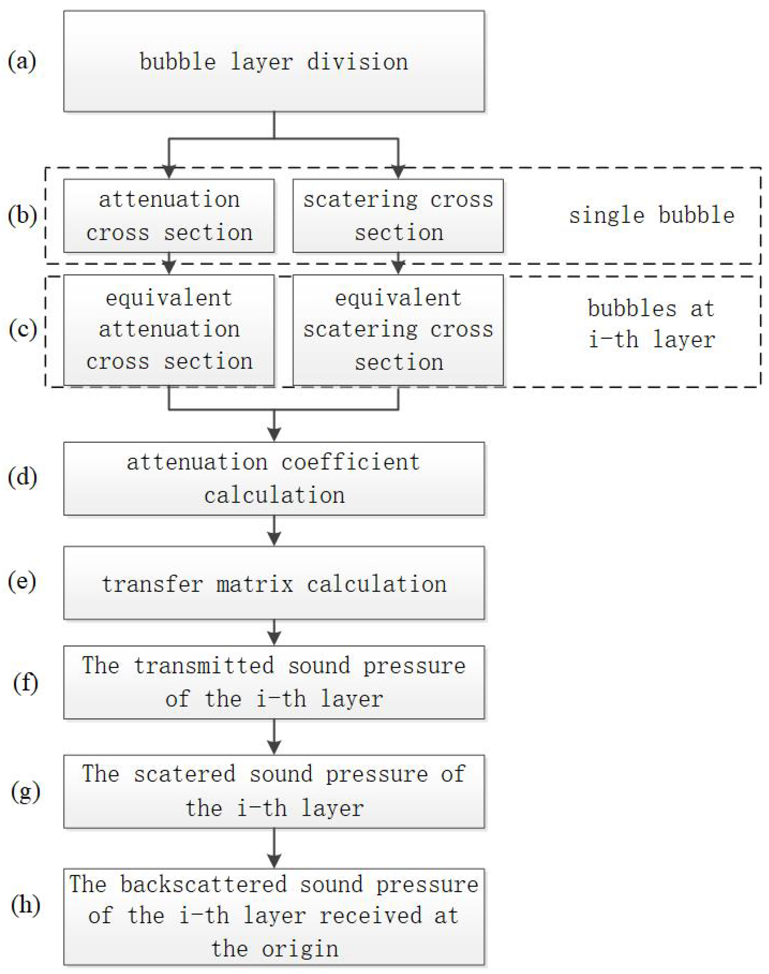
2.3. Multiple Bubble Layer Model

For non-homogeneous ocean bubbles, we assume that the scattering of each bubble is isotropic, and all calculations are performed in the frequency domain. In the bubbly liquids with non-homogeneous distributed bubbles, as shown in Figure 1, the bubble layer is divided by the layer thickness of $\Delta z$, and a total of $N_i$ layers are divided. Each bubble group is regarded as a whole, and the bubble radius is distributed in $R=\left[\begin{array}{cccccc}{R}_1& R_2& \cdots & R_j& \cdots & R_M\end{array}\right]$. The number of bubbles with a radius of $R_j$ in the ith layer is represented as $n\left(i,R_j\right)$, $1\le i\le N_i$. The sound source position is taken as the origin. The one-dimensional case is considered, that is, plane wave propagation. Furthermore, only the scattering in the axial direction is considered, i.e., forward scattering and backward scattering.

Then, the equivalent attenuation cross section $S_e\left(i,f\right)$ of the i-th bubble can be written in the form of a matrix as

$$\left[\begin{array}{c}{S}_e\left(1,f\right)\\ S_e\left(2,f\right)\\ ⋮\\ S_e\left(N_i,f\right)\end{array}\right]=\left[\begin{array}{cccc}n\left(1,R_1\right)& n\left(1,R_2\right)& \cdots & n\left(1,R_M\right)\\ n\left(2,R_1\right)& n\left(2,R_2\right)& \cdots & n\left(2,R_M\right)\\ ⋮& ⋮& \ddots & ⋮\\ n\left(N_i,R_1\right)& n\left(N_i,R_2\right)& \cdots & n\left(N_i,R_M\right)\end{array}\right]\left[\begin{array}{c}{\sigma }_e\left(R_1,f\right)\\ {\sigma }_e\left(R_2,f\right)\\ ⋮\\ {\sigma }_e\left(R_M,f\right)\end{array}\right].$$

(11)

Similarly, the equivalent scattering cross section $S_s\left(i,f\right)$ of the i-th bubble can be written as

$$\left[\begin{array}{c}{S}_s\left(1,f\right)\\ S_s\left(2,f\right)\\ ⋮\\ S_s\left(N_i,f\right)\end{array}\right]=\left[\begin{array}{cccc}n\left(1,R_1\right)& n\left(1,R_2\right)& \cdots & n\left(1,R_M\right)\\ n\left(2,R_1\right)& n\left(2,R_2\right)& \cdots & n\left(2,R_M\right)\\ ⋮& ⋮& \ddots & ⋮\\ n\left(N_i,R_1\right)& n\left(N_i,R_2\right)& \cdots & n\left(N_i,R_M\right)\end{array}\right]\left[\begin{array}{c}{\sigma }_s\left(R_1,f\right)\\ {\sigma }_s\left(R_2,f\right)\\ ⋮\\ {\sigma }_s\left(R_M,f\right)\end{array}\right].$$

(12)

In the i-th layer, the relationship between the attenuation coefficient caused by bubbles and the equivalent attenuation cross section is written as

$${\alpha }_b\left(i,f\right)=4.34S_e\left(i,f\right)\left(\mathrm{dB}/\mathrm{m}\right).$$

(13)

The attenuation coefficient in the ocean has an empirical formula

$${\alpha }_f\left(f\right)={\displaystyle \frac{0.109f^2}{1+f^2}}+{\displaystyle \frac{40.7f^2}{4100+f^2}}+3.01\times {10}^{-4}{f}^2\left(\mathrm{dB}/\mathrm{km}\right).$$

(14)

Assuming that the sound pressure amplitude of the i-th layer is $P\left(i,f\right)$, the relationship between the bubble scattering sound pressure and the equivalent scattering cross section is

$$P_s\left(i,f\right)={\displaystyle \frac{S_s\left(i,f\right)P\left(i,f\right)}{4\pi }}.$$

(15)

Define the transfer matrix as

$$P_s\left(i,f\right)=\lambda \left(i,f\right)P\left(i,f\right).$$

(16)

Furthermore, substituting Equation (16) into Equation (15), we can obtain the transfer matrix as

$$\lambda \left(i,f\right)={\displaystyle \frac{S_s\left(i,f\right)}{4\pi }}.$$

(17)

Then, the sound pressure reaching the i-th layer can be expressed as the sum of the transmitted sound pressure and the scattered sound pressure of the $\left(i-1\right)$-th layer, written as

$$P\left(i,f\right)=P\left(i-1,f\right)\left[e^{-{\alpha }_f\left(f\right)}{10}^{-{\alpha }_b\left(m,f\right)/\phantom{-{\alpha }_b\left(m,f\right)20}20}+\lambda \left(i,f\right)\right].$$

(18)

Define $P\left(0,f\right)$ as the excitation sound pressure at the origin, iterate Equation (18), and write

$$P\left(i,f\right)=P\left(0,f\right)\underset{m=1}{\overset{i}{\Pi }}\left[e^{-{\alpha }_f\left(f\right)}{10}^{-{\alpha }_b\left(m,f\right)/\phantom{-{\alpha }_b\left(m,f\right)20}20}+\lambda \left(m,f\right)\right].$$

(19)

Therefore, the backscatter of the i-th layer can be written as

$$P_s\left(i,f\right)=P\left(i,f\right)\lambda \left(i,f\right).$$

(20)

Furthermore, substituting Equations (17) and (19) into Equation (20), we have

$$P_s\left(i,f\right)=P\left(0,f\right)\lambda \left(i,f\right)\underset{m=1}{\overset{i}{\Pi }}\left[e^{-{\alpha }_f\left(f\right)}{10}^{-{\alpha }_b\left(m,f\right)/\phantom{-{\alpha }_b\left(m,f\right)20}20}+\lambda \left(m,f\right)\right].$$

(21)

Each layer of bubbles can be regarded as a whole, and the scattering of it propagates in the form of a point source. Therefore, the backscatter of the i-th layer received at the origin is

$${\widehat{P}}_s\left(i,f\right)={\displaystyle \frac{P_s\left(i,f\right)}{i\Delta z}}\underset{m=1}{\overset{i}{\Pi }}\left[e^{-{\alpha }_f\left(f\right)}{10}^{-{\alpha }_b\left(m,f\right)/\phantom{-{\alpha }_b\left(m,f\right)20}20}+\lambda \left(m,f\right)\right].$$

(22)

Moreover, substituting Equation (21) into Equation (22),

$${\widehat{P}}_s\left(i,f\right)={\displaystyle \frac{P\left(0,f\right)\lambda \left(i,f\right)}{i\Delta z}}{\left(\underset{m=1}{\overset{i}{\Pi }}\left[e^{-{\alpha }_f\left(f\right)}{10}^{-{\alpha }_b\left(m,f\right)/\phantom{-{\alpha }_b\left(m,f\right)20}20}+\lambda \left(m,f\right)\right]\right)}^2.$$

(23)

3. Simulation

From the above theory, we can know that the simulation process is shown in Figure 2.

The common parameters of bubbly liquids used in the simulation are shown in

Table 1. The common parameters of bubbles and media.

Parameter	Value	Definition
$c_l$	1480 $\mathrm{m}/\phantom{\mathrm{m}\mathrm{s}}\mathrm{s}$	sound speed in a pure water
$c_g$	340 $\mathrm{m}/\phantom{\mathrm{m}\mathrm{s}}\mathrm{s}$	sound speed of air
$\gamma$	1.4	the specific heat ratio of air
${\rho }_l$	998 $\mathrm{g}/\phantom{\mathrm{g}\mathrm{c}{\mathrm{m}}^3}\mathrm{c}{\mathrm{m}}^3$	the density of water
${\rho }_g$	1.29 $\mathrm{g}/\phantom{\mathrm{g}\mathrm{c}{\mathrm{m}}^3}\mathrm{c}{\mathrm{m}}^3$	the density of air
${\eta }_s$	$1\times {10}^{-3}$ $\mathrm{Pa}\times \mathrm{s}$	the shear viscosity coefficient
$K_g$	$5.6\times {10}^{-5}$	the thermal conductivity
$C_P$	0.24 $\mathrm{J}/\phantom{\mathrm{J}\left(\mathrm{kg}\times \mathrm{K}\right)}\left(\mathrm{kg}\times \mathrm{K}\right)$	the specific heat capacity

.

In this section, we consider the propagation of single frequency sound waves in bubbly liquids. In the computational domain, it is considered to be excited at a pure frequency f; f is set to sweep from 20 kHz to 180 kHz. The initial pressure $p_0=10$ kPa, and the sound pressure level is 200 dB.

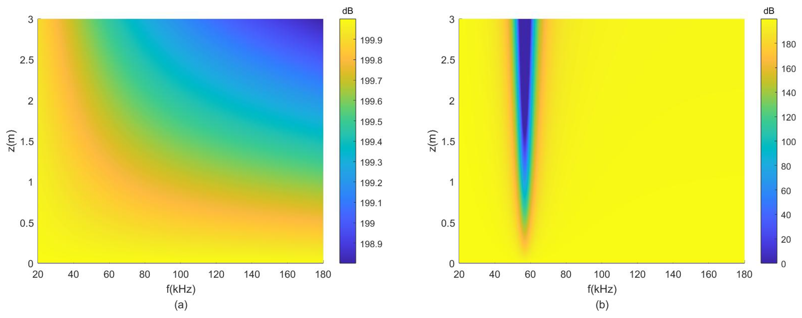
3.1. Homogeneous Bubbles

For homogeneous bubbles, we set the bubble radius $R_0$ = 60 $\mathsf{\mu }$m, and the volumetric void fraction is $Z=1\times {10}^{-6}$, which means the percentage of gas in the mixture. The comparison between the multiple bubble layer model and the results of the coupling model is shown in Figure 3. We can see that the difference between the multiple bubble layer model and the coupling model is less than 2 dB. Compared with the numerical method used in the coupling model, the multiple bubble layer model is a semi-numerical and semi-analytical method. The computational costs of the multiple bubble layer model and the coupling model are shown in

Table 2. Computational cost of the multiple bubble layer model and the coupling model.

Model	Distance (m)	Calculation Time (s)	Required Memory (GB)
the multiple bubble layer model	6	0.47	0.1083
the coupling model	6	1.34	0.1194
the multiple bubble layer model	60	3.83	1.0826
the coupling model	60	1597.19	11.9226

. When the calculation distance is 6 m, the calculation speed of the multiple bubble layer model is 2.85 times that of the coupling model, and the difference in calculation speed is greater with the increase in distance. Moreover, the memory occupied by the multiple bubble layer model is proportional to the distance, while the memory occupied by the coupling model is proportional to the square of the calculated distance. Therefore, the calculation process of the multiple bubble layer model is simpler, and the calculation speed is greatly accelerated, and a longer distance can be calculated in the simulation without occupying much computing memory.

Keeping the volumetric void fraction $Z=1\times {10}^{-6}$ and changing the bubble radius, the attenuation coefficients of bubble layers with different radii under different frequency excitations can be obtained, as shown in Figure 4. It can be seen from the Figure 4 that the attenuation coefficient of the bubble layer reaches its maximum value at the resonance frequency; the highest can reach 350 dB/m. This is because the bubbly liquids have high sound absorption attenuation; bubbles compress and expand under the action of sound waves, causing the temperature inside bubbles to rise and fall, and exchanging heat energy with the surrounding medium, thus converting acoustic energy into heat energy and consuming it. In addition, the viscous effect of bubbly liquids on the compression and expansion of bubbles also loses some energy. In addition, as a resonant cavity, bubbles strongly scatter the incident sound waves, resulting in the obvious attenuation of the incident sound energy. However, in pure water, the attenuation coefficient is a function of frequency, and below 180 kHz, the attenuation coefficient is less than 1 dB. This is also one of the important reasons why bubbly liquids have attracted attention. As the bubble radius increases, the resonance frequency gradually decreases. When the volumetric void fraction remains unchanged, the layer containing larger bubbles have a smaller attenuation coefficient. Moreover, there is still a large attenuation coefficient in the range of 10 kHz near the resonant frequency, which shows that ignoring the influence of non-resonant bubble vibration in classical theory will lead to large errors, and the multiple bubble layer model solves this problem very well.

When the bubble radius $R_0$ = 60 $\mathsf{\mu }$m, the volumetric void fraction is $Z=1\times {10}^{-6}$. The results of the multiple bubble layer model are shown in Figure 5b, where colors mean amplitudes. The results are compared with those in the case of $Z=0$, in the case of pure water, as shown in Figure 5a. Combined with Figure 4, we can see that adding a small amount of bubbles can greatly increase the attenuation coefficient of the medium at a specific frequency, while at other excitations far from the resonant frequency, the attenuation is the same as pure water. This is the effect of bubble vibration, which is a characteristic of the bubble layer.

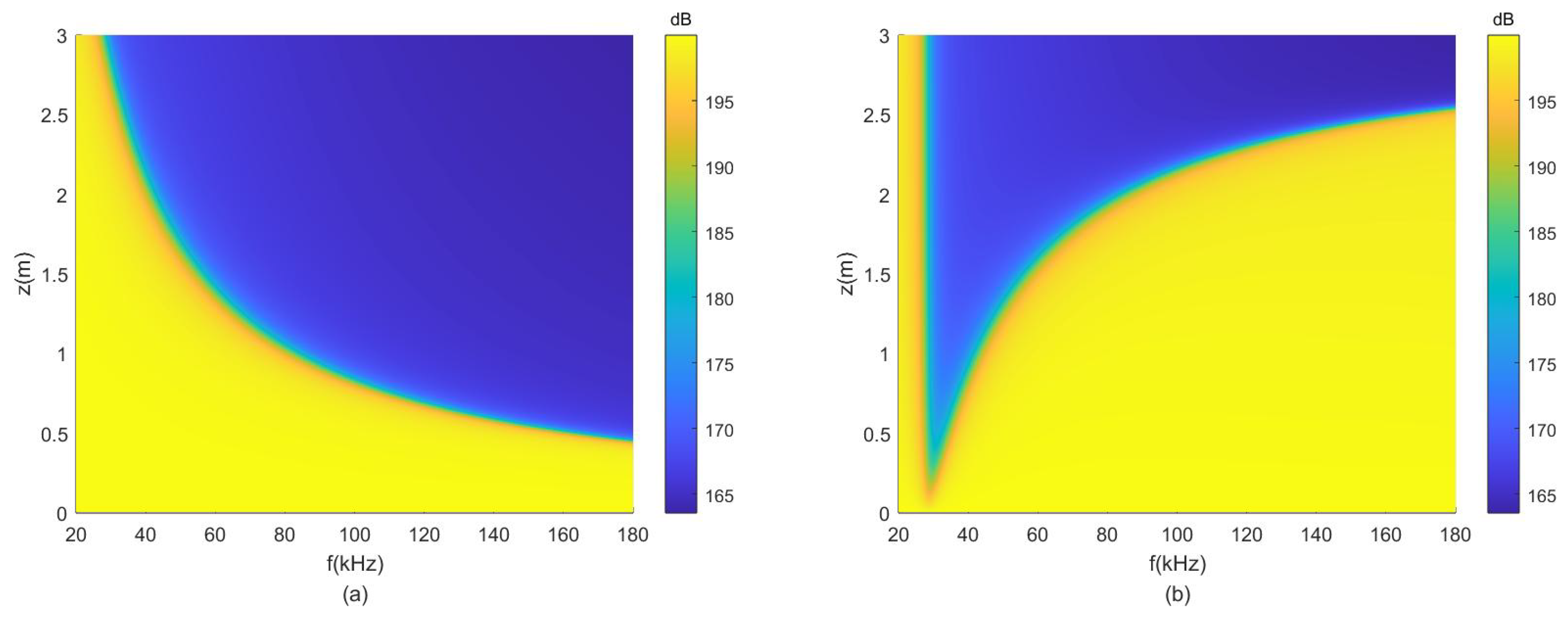
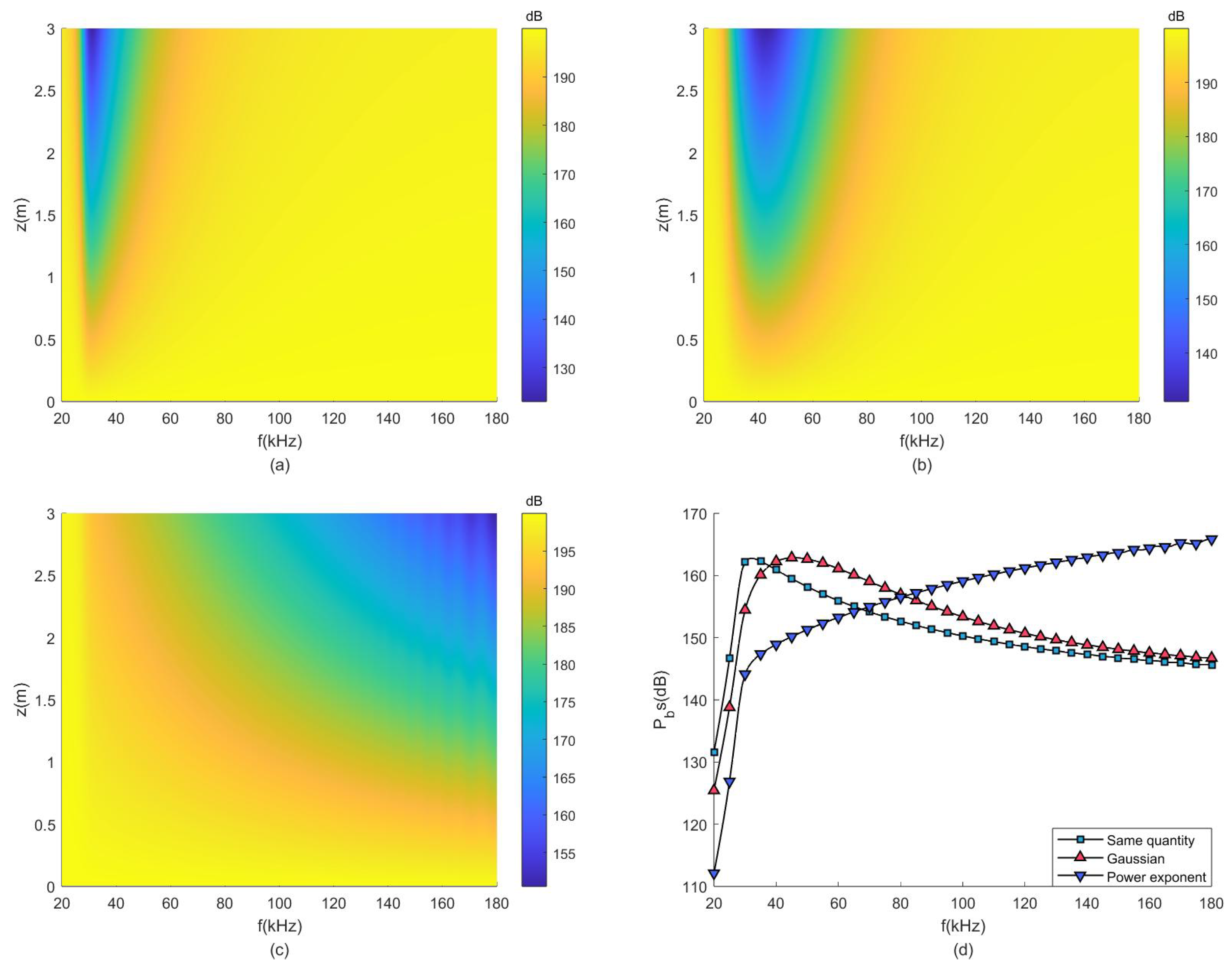
3.2. Non-Homogeneous Bubbles

For non-homogeneous bubbles, first, we set them to gradient bubble layers. The volumetric void fraction $Z=1\times {10}^{-6}$. In the first case, the bubble radius gradually increases, and the result is shown in Figure 6a. In the second case, the bubble radius gradually decreases, and the result is shown in Figure 6b. The volumetric void fraction is kept constant for comparison purposes in this paper. Compared with Figure 4, even if the volumetric void fraction is the same, the difference in bubble distribution will seriously affect the distribution of the sound field. However, since the bubble layer structures of the increasing and decreasing distributions are the same, the positions of the bubble layers are different, and the total attenuation differs by less than 5 dB. This result shows that the position of the bubble layer affects the spatial distribution of the sound pressure but has no obvious effect on the overall attenuation of the bubbly liquids. This result also proves that the classic equivalent medium method has wide applicability and accuracy in the attenuation calculation of linear acoustics.

In order to demonstrate the influence of the bubble layer structure, we set up three bubble distributions here.

1.

Same quantity distribution;

$$n\left(R\right)=A_1.$$

(24)

2.

Gaussian distribution;

$$n\left(R\right)={\displaystyle \frac{A_2}{\sqrt{2\pi }\sigma }}{e}^{-{\displaystyle \frac{{(R-r_0)}^2}{2{\sigma }^2}}},$$

(25)

where $r_0$ = 60 $\mathsf{\mu }$m, $\sigma =0.4r_0$.

3.

Power exponent distribution.

$$n\left(R\right)=A_3{R}^m,$$

(26)

where m represents the power index, here, we set $m=-4$.

The following is the discussion of the relationship between the bubble distribution and the acoustic field distribution. The volumetric void fraction is also kept $Z=1\times {10}^{-6}$ here. In Figure 7, the acoustic field distribution under three bubble distributions is simulated, respectively. The multiple bubble layer model regards each layer of bubbles as a point source, so the value of the backscatter can be further calculated. Finally, the backscatter received at the origin is shown in Figure 7d. Among the three distributions, same quantity distribution has the largest attenuation coefficient and has a greater attenuation for low frequencies. Meanwhile, power exponent distribution has the smallest attenuation coefficient, which differs from Same quantity distribution by more than 20 dB, and has a greater attenuation for high frequencies. Gaussian distribution is similar to the single distribution, but the resonant frequency of the bubble layer is shifted toward low frequencies, compared to the resonant frequency corresponding to the radius of the concentrated distribution of the bubble layer. From 20 kHz to 30 kHz, the bubble backscattering increases with increasing frequency. The resonant frequencies of the bubble layers of the same quantity and gaussian distribution are both at low frequencies, resulting in the maximum backscattering of the bubbles at low frequencies and the minimum transmission. The backscattering of the bubble layer of power exponent distribution gradually increases with increasing frequency while the transmission gradually decreases.

4. Conclusions

A semi-numerical and semi-analytical calculation method for underwater sound fields containing non-homogeneous bubbles is proposed in this paper. Compared with the numerical method used in the coupling model, the accuracy of the model has been proven. From the simulation results, it can be seen that

• Adding a small amount of bubbles can greatly increase the attenuation coefficient of the medium at a specific frequency;
• The position of the bubble layer affects the spatial distribution of the sound pressure but has no obvious effect on the overall attenuation of the bubbly liquids;
• Bubble distribution is the main factor affecting sound propagation. Under the same volumetric void fraction, the same quantity and Gaussian-distributed bubbles have the largest backscattering and the smallest transmittance at low frequencies. The backscattering of the power exponentially distributed bubble layer increases with the increase in frequency, and the transmittance decreases gradually.

The beneficial effects of this model can be summarized as follows:

1.

It can adapt to various conditions of the non-homogeneous distribution of bubbles, providing strong support for the subsequent study of the spatial propagation law of sound waves in underwater non-homogeneous bubble sound fields;

2.

The attenuation of the medium itself and the attenuation caused by bubble vibration work together, and the influence of bubble scattering is added to the forward propagation, which is more realistic than the previous simulation model under ideal conditions and corrects the errors caused by ignoring these effects;

3.

As a special underwater scatterer, bubbles are propagated in the form of point sound sources in this model, which can better reflect the influence of bubble group vibration and scattering on sound wave propagation and realize the calculation of backscattered sound pressure of non-homogeneous distributed bubbles;

4.

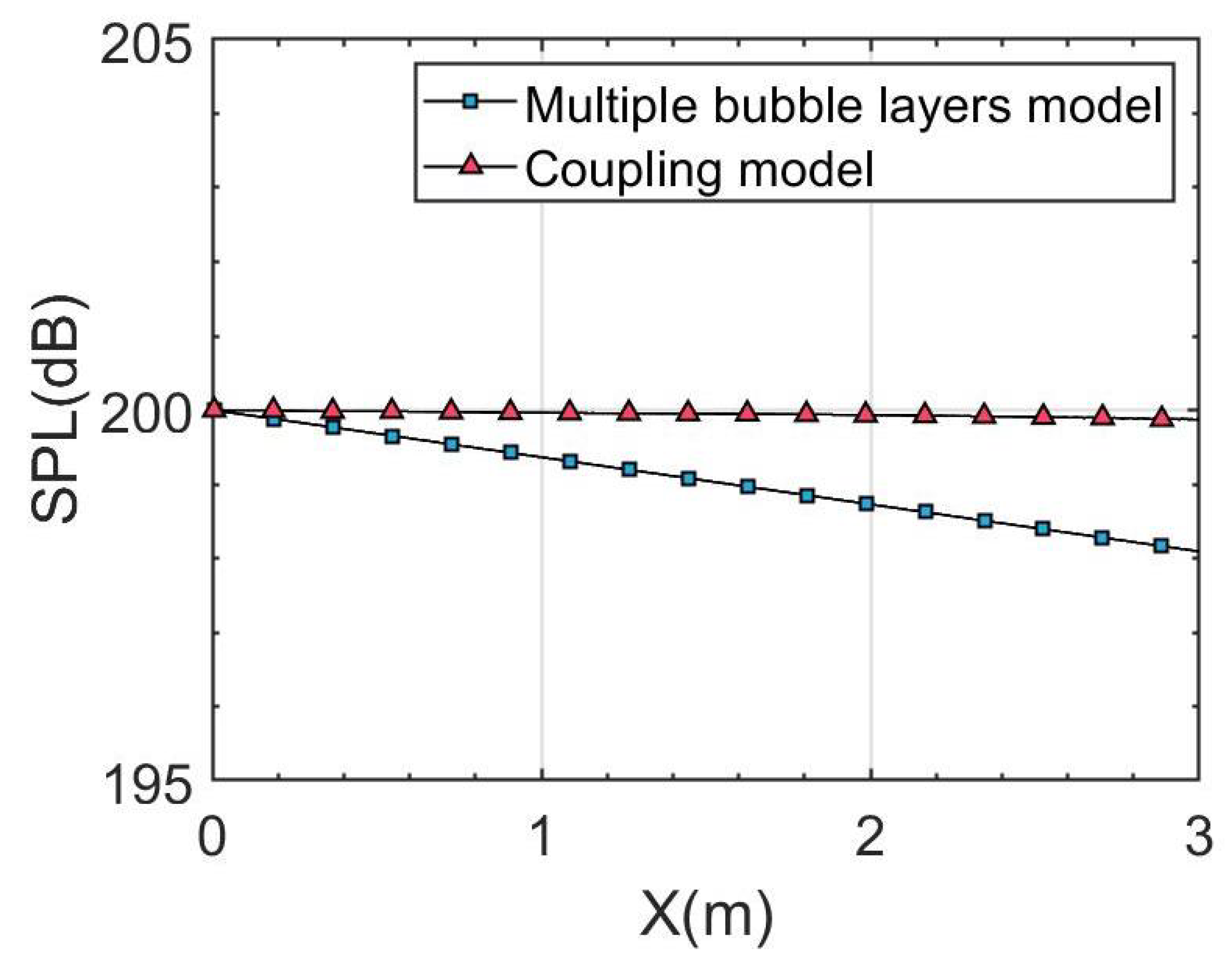
When the calculation distance is 6 m, the calculation speed of the multiple bubble layer model is 2.85 times that of the coupling model, and the difference in calculation speed is greater with the increase in distance. Moreover, the memory occupied by the multiple bubble layer model is proportional to the distance, while the memory occupied by the coupling model is proportional to the square of the calculated distance.

References

- Commander, K.W. Linear pressure waves in bubbly liquids: Comparison between theory and experiments. J. Acoust. Soc. Am. 1989, 85, 732–746. [Google Scholar] [CrossRef]
- Commander, K.W. Off-resonance contributions to acoustical bubble spectra. J. Acoust. Soc. Am. 1989, 85, 2665–2669. [Google Scholar] [CrossRef]
- Sornette, D. Acoustic wave propagation in one-dimensional stratified gas–liquid media: The different regimes. J. Acoust. Soc. Am. 1991, 92, 296–308. [Google Scholar] [CrossRef]
- Prosperetti, A. Active and passive acoustic behavior of bubble clouds at the ocean’s surface. J. Acoust. Soc. Am. 1993, 93, 3117–3127. [Google Scholar] [CrossRef]
- Prosperetti, A. A general derivation of the subharmonic threshold for non-linear bubble oscillations. J. Acoust. Soc. Am. 2013, 133, 3719–3726. [Google Scholar] [CrossRef]
- Lyons, A.P. Predictions of the acoustic response of free-methane bubbles in muddy sediments. J. Acoust. Soc. Am. 1994, 96, 3217–3218. [Google Scholar] [CrossRef]
- Ye, Z. Acoustic dispersion and attenuation relations in bubbly mixture. J. Acoust. Soc. Am. 1995, 98, 1629–1636. [Google Scholar] [CrossRef]
- Shagapov, V.S.H. Acoustic waves in a liquid with a bubble screen. Shock Waves 2003, 13, 49–56. [Google Scholar] [CrossRef]
- Shagapov, V.S.H. Refraction and reflection of sound at the boundary of a bubbly liquid. Acoust. Phys. 2015, 61, 37–44. [Google Scholar] [CrossRef]
- Vanhille, C. Nonlinear ultrasonic waves in bubbly liquids with nonhomogeneous bubble distribution: Numerical experiments. Ultrason. Sonochem. 2009, 16, 669–685. [Google Scholar] [CrossRef]
- Vanhille, C. Simulation of nonlinear ultrasonic pulses propagating through bubbly layers in a liquid: Filtering and characterization. J. Comput. Acoust. 2011, 18, 47–68. [Google Scholar] [CrossRef]
- Vanhille, C. Two-dimensional numerical simulations of ultrasound in liquids with gas bubble agglomerates: Examples of bubbly-liquid-type acoustic metamaterials (blamms). Sensors 2017, 17, 173. [Google Scholar] [CrossRef]
- Vanhille, C. Numerical simulations of the nonlinear interaction of a bubble cloud and a high intensity focused ultrasound field. Acoustics 2019, 1, 825–836. [Google Scholar] [CrossRef]
- Chong, K.J.Y. The effects of coupling and bubble size on the dynamical-systems behaviour of a small cluster of microbubbles. J. Sound Vib. 2010, 329, 687–699. [Google Scholar] [CrossRef]
- Zhang, Y. A generalized equation for scattering cross section of spherical gas bubbles oscillating in liquids under acoustic excitation. J. Fluids Eng. 2013, 135, 091301. [Google Scholar] [CrossRef]
- Zhang, Y. Effects of mass transfer on damping mechanisms of vapor bubbles oscillating in liquids. Ultrason. Sonochem. 2018, 40, 120–127. [Google Scholar] [CrossRef]
- Zhang, Y. Influences of bubble size distribution on propagation of acoustic waves in dilute polydisperse bubbly liquids. J. Hydrodyn. 2019, 31, 50–57. [Google Scholar] [CrossRef]
- Zhang, Y. Interior non-uniformity of acoustically excited oscillating gas bubbles. J. Hydrodyn. 2019, 31, 725–732. [Google Scholar] [CrossRef]
- Zhao, J. Study on the Acoustic Reflection Characteristics of Underwater Bubble Layer. Master’s Thesis, Harbin Engineering University, Harbin, China, 2014. [Google Scholar]
- Sun, J. Study on the Acoustic Transmission Characteristics of Underwater Bubble Curtain. Master’s Thesis, Harbin Engineering University, Harbin, China, 2015. [Google Scholar]
- Leighton, T.G. Acoustic propagation in gassy intertidal marine sediments: An experimental study. J. Acoust. Soc. Am. 2021, 150, 2705–2716. [Google Scholar] [CrossRef]
- Gubaidullin, D.A. Reflection of an acoustic wave from a bubble layer of finite thickness. Dokl. Phys. 2016, 61, 499–501. [Google Scholar] [CrossRef]
- Gubaidullin, D.A. Acoustic wave incidence on a multilayer medium containing a bubbly fluid layer. Fluid Dyn. 2017, 52, 107–114. [Google Scholar] [CrossRef]
- Gubaidullin, D.A. Interaction of acoustic waves with bubbly layer with uneven distribution of bubbles. Lobachevskii J. Math. 2019, 40, 751–756. [Google Scholar] [CrossRef]
- Gubaidullin, D.A. Reflection and transmission of acoustic wave through a multifractional bubble layer. High Temp. 2020, 58, 97–100. [Google Scholar] [CrossRef]
- Liu, R. The effects of bubble scattering on sound propagation in shallow water. J. Mar. Sci. Eng. 2021, 9, 1441. [Google Scholar] [CrossRef]
- Bulanov, V.A. On sound scattering and acoustic properties of the upper layer of the sea with bubble clouds. J. Mar. Sci. Eng. 2022, 10, 872. [Google Scholar] [CrossRef]
- Gusev, V.A. Nonlinear sound in a gas-saturated sediment layer. Acoust. Phys. 2015, 61, 152–164. [Google Scholar] [CrossRef]
- Mantouka, A. Modelling acoustic scattering, sound speed, and attenuation in gassy soft marine sediments. J. Acoust. Soc. Am. 2016, 140, 274–282. [Google Scholar]
- Zheng, G. Sound speed, attenuation, and reflection in gassy sediments. J. Acoust. Soc. Am. 2017, 142, 530–539. [Google Scholar] [CrossRef]
- Li, J. Acoustic and optical determination of bubble size distributions—Quantification of seabed gas emissions. Int. J. Greenh. Gas Control 2021, 108, 103313. [Google Scholar] [CrossRef]
- Kanagawa, T. Nonlinear wave equation for ultrasound beam in nonuniform bubbly liquids. J. Fluid Sci. Technol. 2011, 6, 279–290. [Google Scholar] [CrossRef]
- Lesnik, S. Modeling acoustic cavitation with inhomogeneous polydisperse bubble population on a large scale. Ultrason. Sonochem. 2022, 89, 106060. [Google Scholar] [CrossRef] [PubMed]
- Wildt, R. (Ed.) Acoustic theory of bubbles. In The Physics of Sound in the Sea; NDRC Summary Technical Report Div. 6 8; US Navy: Washington, DC, USA, 1946. [Google Scholar]