In Situ Measurement of Deep-Sea Salinity Using Optical Salinometer Based on Michelson Interferometer

Abstract

Ocean salinity plays an important role in oceanographic research as one of the fundamental parameters. An optical salinometer based on the Michelson interferometer (MI) suitable for in situ measurement in deep-sea environments is proposed in this work, and it features real-time calibration and multichannel multiplexing using the frequency modulated continuous wave (FMCW) technique. The symmetrical sapphire structure used to withstand deep-sea pressure can not only achieve automatic temperature compensation, but also counteract the changes in optical path length under deep-sea pressure. A model formula suitable for optical salinity demodulation is proposed through the nonlinear least squares fitting method. In vertical profile testing, the optical salinometer demonstrated remarkable tracking performance, achieving an error of less than 0.001 psu. The sensor displays a stable salinity demodulation error within ±0.002 psu during a three-month long-term test at a depth of 4000 m. High stability and resolution make this optical salinometer have broad development prospects in ocean observation.

1. Introduction

Salinity, being a pivotal parameter of seawater, plays a crucial role in various scientific inquiries, including the examination of the exploration of marine biological activities, the monitoring of seawater quality, and the modeling of ocean dynamics and climate change [1,2,3]. The change in seawater salinity is closely related to natural phenomena. In circumstances where precipitation exceeds evaporation, a reduction in salinity is observed. In high-latitude waters, the formation of ice excludes salt from the water, thereby increasing the salinity of the remaining seawater. Furthermore, the monitoring of salinity is of significant interest. The long-term monitoring of seawater salinity allows us to gain deep insights into the complex interplay of physical, chemical, and biological processes within marine environments. This effort aids in assessing the health of marine ecosystems, enabling the timely identification of ecological issues and the implementation of protective measures. Additionally, the quantitative planning of areas for the exploitation of fishery resources can enhance the efficiency of the desalination process, thereby promoting the sustainable development of the marine economy. The advancement in salinity sensing technology has spanned from the calorimetric salinity method [4] to the Practical Salinity Scale established in 1978 [5], ultimately culminating in the TEOS-10 equation of state for seawater [6]. In the field of oceanography, salinity is further divided into absolute salinity (S_A) and practical salinity (S_P), with their units being grams per kilogram (g/kg) and Practical Salinity Unit (psu), respectively. In order to establish a connection with previous data, the correlation between practical salinity and absolute salinity was established by introducing the reference salinity (S_R) [7], as demonstrated in Equations (1) and (2). This methodology enables the conversion between psu and g/kg.

$$S_R=(35.16504/35.000)S_P \mathrm{g}/\mathrm{kg}$$

(1)

$$S_A=S_R+\delta S_A=S_A(S_P,\phi ,\varphi ,p)$$

(2)

where $\phi$ is longitude, $\varphi$ is latitude, p is the seawater pressure at the sampling depth, and $\delta S_A$ is absolute salinity deviation [8].

While the multi-electrode conductivity method, grounded in the Practical Salinity Scale-1978 (PSS-78), has been extensively employed for salinity measurements, it nonetheless has encountered challenges. The calculation of salinity by conductivity is confined to measuring ionized substances present in seawater, thereby partially neglecting non-conductive dissolved substances [7]. This includes dissolved inorganic compounds [8], as well as dissolved organic matter (DOM) [9] and dissolved organic nitrogen (DON) [10]. This means that salinity measurements based on conductivity methods may not accurately sense the salinity of seawater.

Recent advancements in empirical formulas (M-S equation) that correct the optical temperature, salinity, depth, wavelength, and refractive index (RI) [11] have paved the way for optical-based salinity sensing. However, the challenging high-pressure environment of the deep sea poses significant obstacles for sophisticated optical instrumentation [12]. Furthermore, studies in the western North Pacific have shown very small changes in salinity of around 2 × 10⁻⁴ g/kg in 100 km [13]. Therefore, the advancement of deep-sea exploration has underscored the necessity for sensors that exhibit long-term stability and precision in measuring seawater salinity [14,15].

Fiber optic RI sensors have been widely developed in recent years. They hold promising potential as RI sensors for ocean salinity measurements [16,17,18,19,20]. However, they encounter significant challenges under the extreme pressures prevalent in such settings, ultimately leading to compromised accuracy [12].

In the realm of technology for measuring seawater salinity utilizing optical RI, free spatial optics has emerged as a superior approach, demonstrating exceptional applicability both theoretically during the design and practically during marine testing. Compact RI sensors employing the total internal reflection method have been developed, achieving a resolution of 1.17 × 10⁻⁵ RIU for salinity sensing in shallow waters during ship cruising [21]. However, these sensors exhibit low sensitivity and are unable to withstand the high-pressure environment of the deep sea. A refractometer based on the V-block principle [22] was proposed to measure the RI of seawater with a resolution of approximately ±4 × 10⁻⁷ RIU, which is equivalent to a salinity resolution of ±0.002 g/kg. Furthermore, a sea trial of 2000 m was conducted and exhibited salinity measurements with a resolution of 0.001 g/kg [23]. A salinity sensor based on the principle of optical interference has been proposed [13], utilizing silica glass as the reference path and a high-resolution commercial thickness gauge as the demodulation system. However, the asymmetric interference arms formed by seawater and quartz might need complex temperature and pressure compensations, due to the large different thermal optical coefficients between seawater and quartz, as well as the pressure-induced stress on the quartz. An optical salinometer, relying on the self-calibration of standard seawater, has demonstrated a salinity resolution of 0.0003 psu in a laboratory pressure tank [12]. While exhibiting pressure-resistant attributes, this approach also faces challenges in terms of synchronization of temperature response time in the two arms. We previously demonstrated a salinity sensor based on a Fabry–Perot interferometer, which uses a laser dithering frequency-locking technique to precisely lock the laser frequency at the peak resonance [24,25]. However, the method of adjusting the wavelength of the laser by applying a feedback voltage to the laser does not allow for simultaneous multiplexed sensing and is not conducive to the integration of salinity sensors with temperature and pressure sensors.

Certainly, despite progress in spatial optical RI-based seawater salinity measurement, attaining high precision, stability, and long-term reliability in the deep sea faces daunting obstacles due to its extreme conditions. To address these challenges, ocean sensor design should prioritize the following aspects: (1) enhancing pressure resistance and corrosion resistance; (2) improving sensor sensitivity and resolution; (3) enabling multi-parameter synchronous measurement; (4) ensuring long-term stability and reliability.

We introduce a novel free spatial-based optical Michelson interferometer (MI) salinity sensor designed to withstand the extreme pressures encountered in deep-sea environments. In order to evaluate the structural pressure resistance of the probe, simulations were conducted utilizing COMSOL6.0 software to model the deformation of its optical sapphire window under simulated deep-sea pressure conditions. Furthermore, Fluent 2019R2 software was employed to simulate the flow velocity of surrounding seawater during the vertical descent profile of the salinometer, thereby providing theoretical guidance for the exchange of seawater in the flow channel of the probe. An accurate salinity demodulation model was developed through the application of the nonlinear least squares fitting method. The overall performance of this optical pressure-resistant salinity sensor was subjected to rigorous evaluation across the full ocean depth range through the implementation of sea trials.

2. Design and Simulations of the MI Probe

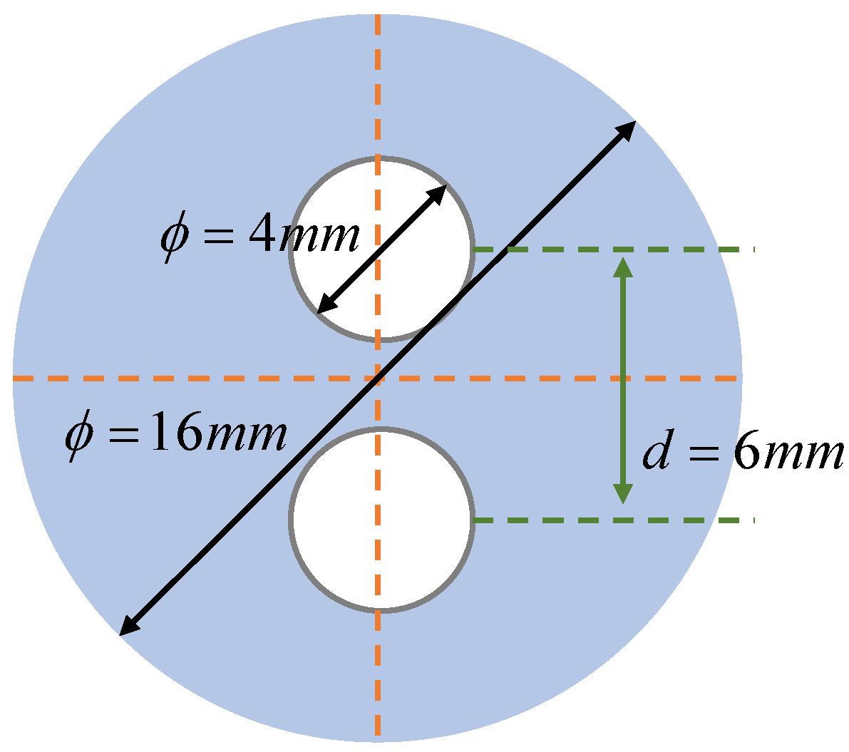
2.1. Design of the MI Probe

The probe is depicted in Figure 1a,b, which exhibit the probe’s 3D appearance and internal details. Stainless steel 2205 was chosen as the encapsulation material due to its resistance to seawater corrosion and its high Young’s modulus. Optical windows were made of sapphire with high transmittance and were able to withstand deep-sea pressure and water tightness. The MI operates on the principle of double-beam interference, which provides a unique advantage for ocean salinity sensing, such as a dual-channel sapphire symmetric self-compensating structure used to mutually cancel out optical path difference (OPD) variations caused by changes in ambient temperature and pressure.

In Figure 1c, L₁ + L₅ and L₂ + L₆ represent the lengths of the air in the two optical paths, respectively, while L₃ and L₄ represent the lengths of the liquids in the optical paths. The OPD expression for MI is shown in Equation (3).

$$OPD=2[n_{air}(L_1+L_5-(L_2+L_6))+n_{\mathrm{sea}}\cdot (L_3-L_4)]$$

(3)

where n_sea is the RI of seawater, n_air is the RI of air, and $L_i$ (i = 1, 2, 3, 4, 5, 6) is identified in Figure 1c.

The relationship between OPD and resonant wavelength is

$$m\cdot \lambda =OPD$$

(4)

Here, m represents the interference order, and $\lambda$ represents the resonant wavelength. The wavelength Free Spectral Range (FSR) is calculated as follows:

$$FS{R}_{\lambda }\approx {\displaystyle \frac{{\lambda }^2}{OPD}}$$

(5)

It is evident that the FSR mainly depends on the OPD. The OPD can be adjusted by varying the length difference between the two optical paths, either in air or seawater. To ensure proper information acquisition and operation of the laser FMCW and cross-correlation demodulation system, the probe signal must have at least two complete interference signals, equivalent to 1–2 FSRs, at a modulation depth of 0.8 V (corresponding to a wavelength change of 0.4 nm). If the FSR were adjusted solely based on the OPD created by the length of the liquid, it would require approximately 5 mm. This could result in excessive depth of small sapphires in mechanical components, leading to localized stagnant water, which is not conducive to the rapid sensing of liquid environments. Therefore, the presence of air gaps is essential. The sensitivity of an optical salinity sensor is primarily affected by the difference in liquid lengths of the two paths [26]. The sensitivity of the optical salinity sensor designed in this work exhibits a positive correlation with the liquid length difference. By adjusting the liquid length difference, the sensitivity of the system can be increased, thereby improving its ability to detect and measure changes in liquid RI. A greater difference leads to improved sensitivity but concurrently poses challenges, such as the difficulty in liquid flow within the structure. Drawing from extensive practical engineering experience, an optimal air gap length of approximately 9 ± 1 mm was determined, while the liquid length difference was set to −1.6 ± 0.02 mm. These settings strike a balance between sensitivity and liquid flow ease, ensuring optimal performance of the sensing system. The precision of salinity sensing is directly influenced by the consistency of the properties of the seawater clusters examined through the dual optical path. Consequently, we have opted to utilize optics with the smallest feasible dimensions and maintain the radial distance of the dual optical path within a range of 6–8 mm. This compact dual-beam configuration not only maximizes spatial efficiency but also minimizes the potential influence of temperature and salinity gradients on sensing performance, thereby enhancing the overall accuracy and reliability of the sensing system.

2.2. Deformation Simulations of Sapphire Window in Deep Sea

Sapphire is not only part of the pressure-resistant structure, but also part of the optical path as an optical window. Whether sapphire will affect OPD when deformed under pressure is an important question. Two sizes of sapphire (Φ4 × 10 mm and Φ16 × 10 mm) were used in this study. The side view of its placement is shown in Figure 2. Its symmetrical structure can automatically compensate for the optical path difference of sapphire at different temperatures. The finite element method (FEM) by COMSOL6.0 software is used to simulate the compressive deformation of sapphire at the extreme case of 120 MPa, and the simulation results are shown in Figure 3. The compressive deformation is centrally symmetrical, and the contour lines are distributed in a circular ring as shown in Figure 3a. The deformation of the anterior and posterior surfaces, as depicted in Figure 3b, falls within the micrometer scale under compression. The symmetrical structure still satisfies the symmetry condition after compression, thus automatically compensating for the changes in the length of the optical path caused by deformation.

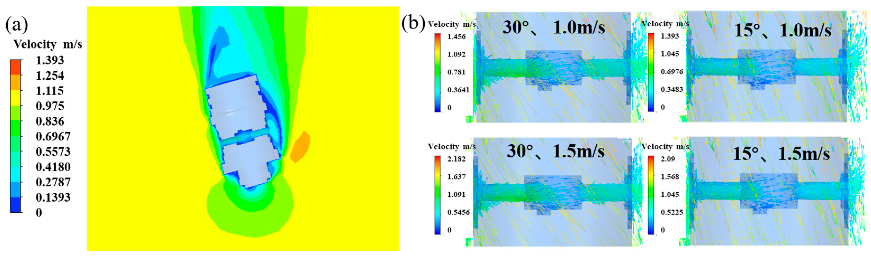
2.3. Simulation of Seawater Flow during Descent Profile

During vertical profiling sea trials, it is intuitive that the ability to exchange fluids quickly has an impact on the performance of the sensors. The uniformity of the measurement samples of the optical and comparison sensors is also a major source of error in the demodulation. Therefore, we constructed the flow model of the sensor during the ocean profile by using Fluent 2019R2 software, and considering the complex shape of the probe structure, we used tetrahedra to divide the fluid region. Since the friction and viscosity of the fluid in the wall region will make the flow much more complicated, a five-layer mesh (with a growth rate of 1.2) is added to the boundary layer of the wall to improve the solution accuracy.

Figure 4a illustrates the flow velocity distribution in the flow field for an inclination angle of 15° and a descent velocity of 1.5 m/s. The distribution of flow velocity in the flow channel at different velocities and inclination angles is shown in Figure 4b, and it can be seen that the flow velocities in the flow channel can all reach one-half of the profile velocity. Assuming that the distance between the tested seawater and the probe is within 10 cm, the liquid exchange time is less than 100 ms. This indicates that the optical salinometer is capable of timely liquid exchange in profile sea trials and can achieve in situ measurements.

3. FMCW System and Calibration of Mathematical Models

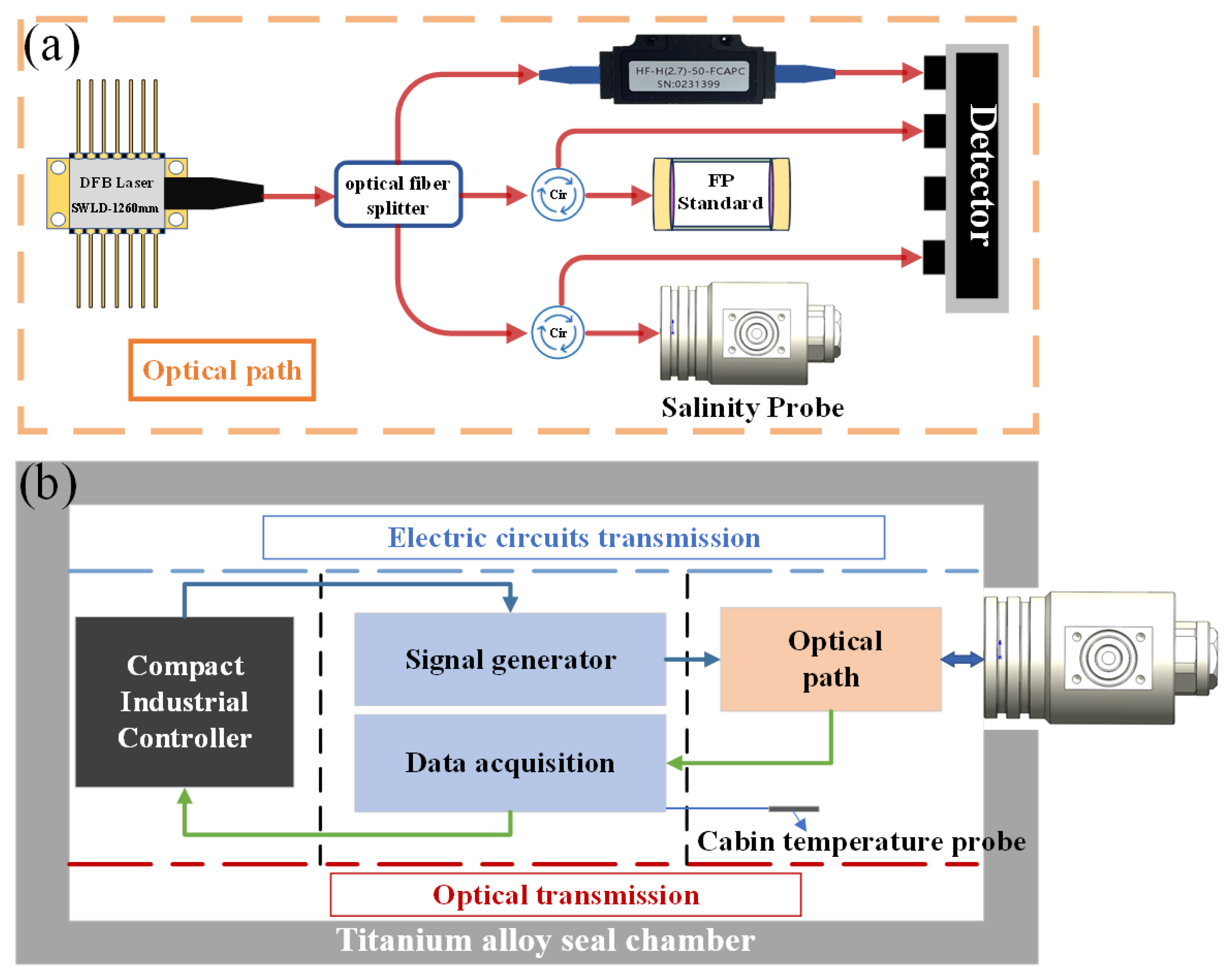
3.1. FMCW System

The FMCW-based MI salinity sensing system is depicted in Figure 5, with Figure 5a presenting the system test interface, Figure 5b outlining the comprehensive optical path of the salinity sensor. Under the precise control of an integrated microcomputer, a signal generator provides a periodic oblique triangular wave signal to modulate the DFB laser, resulting in the emission of a narrow linewidth laser spectrum that varies dynamically over time. The central wavelength of the DFB laser used in this work is 1260 nm with a continuous tuning range of 80 GHz. The laser passes through an optical beam splitter to produce three laser beams with the same wavelength–time relationship. Five percent of the laser intensity is directed towards the HF gas cell; the gas absorption peak was used to serve as a reliable frequency standard for the real-time calibration of the laser’s spectral frequency. Simultaneously, another 5% of the laser intensity enters an FP standard fixture, supported by indium steel material. The selection of low-thermal-expansion materials and their temperature compensation with in-cabin platinum resistors reduce its effect on the system to negligible. As the lasers traversing the gas absorption cell, the FP standard fixture, and the probe share an identical wavelength–time relationship, a cross-correlation algorithm was used to accurately determine the positional difference between the measurement peak and the reference peak [27,28]. This approach effectively reflects changes in the RI of the liquid. The specific demodulation process of the FMCW system is detailed in reference [26]. Figure 6 presents the signal spectra of the essential components. The black solid line illustrates the transmission spectrum of the absorption cell containing HF gas molecules, whereas the red dashed line represents the FP standard fixture. Additionally, the blue dashed line depicts the interference spectrum of an optical salinity probe.

3.2. Sea Trial Equipment and Mathematical Models

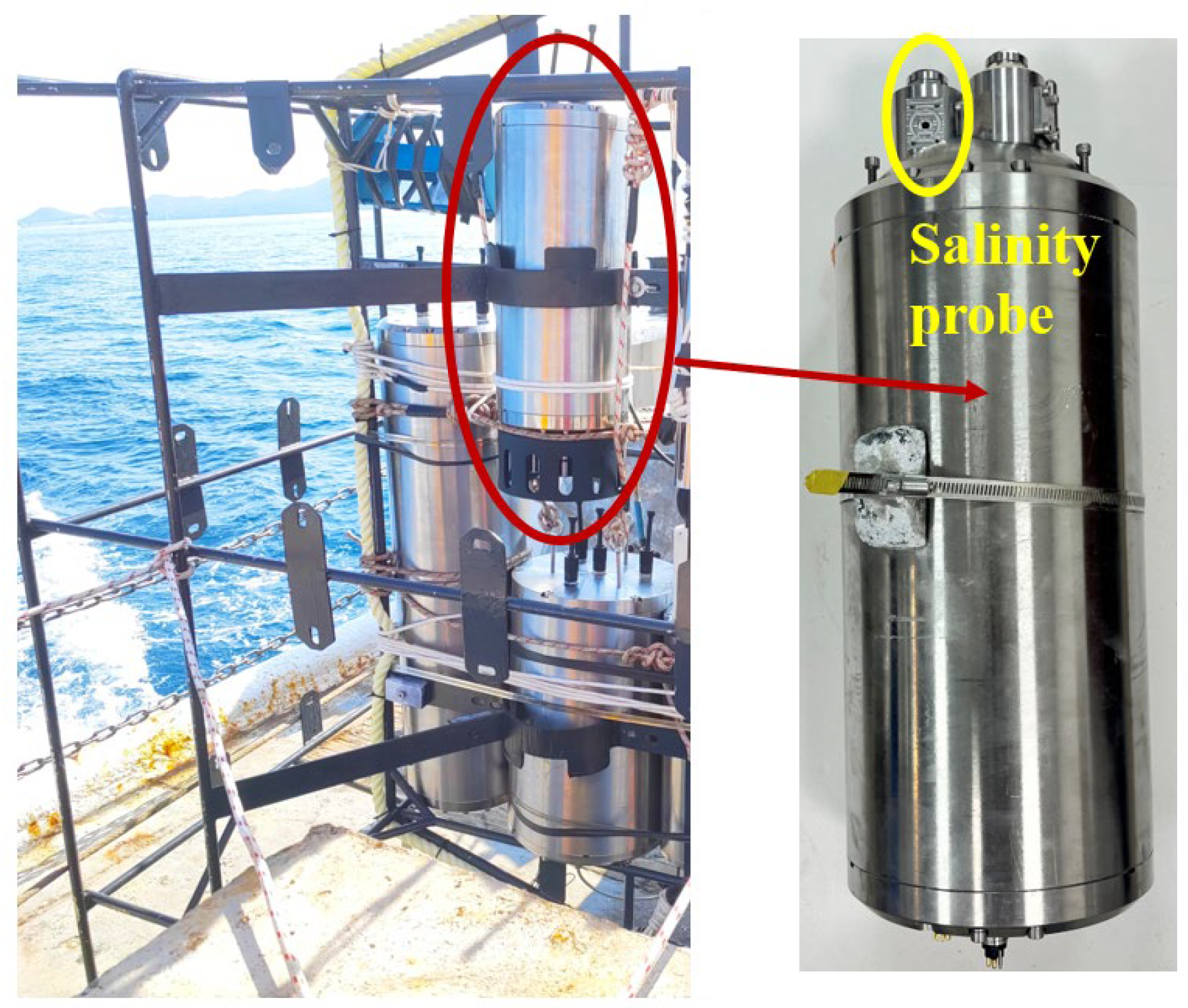
3.2.1. Sea Trial Equipment

The optical salinometer was deployed for a sea trial in the South China Sea with a depth of around 4000 m. The left side of Figure 7 shows the shelf configured for sea trials of the optical sensors. The laser FMCW technique has the characteristic of multiplexing, which can simultaneously measure multiple parameters. The right-hand side in Figure 7 depicts the titanium tank, integrating temperature, salinity, and depth measurements. Notably, the salinity sensor probe is highlighted. The optical salinity sensor was calibrated and tested at the location with a depth of 4000 m in the South China Sea. Before deployment, floating balls and a heavy object were attached to the instrument frame, which then sank to a depth of 4000 m due to the weight of the heavy object. After the test was completed, the acoustic release device sent a signal to disconnect the instrument frame from the heavy object, allowing the frame to float to the surface by the buoyancy provided by the floating balls. For the convenience of long-term underwater testing, the sensor designed in this work is self-contained. The battery uses FANSO’s disposable lithium battery, with the parameters of each battery listed in

Table 1. Battery parameters.

Capacity	Open-Circuit Voltage	Maximum Continuous Discharge Current	Operation Temperature	Size
14,000 mAh	3.66 V	1800 mA	−55 ~ +80 °C	$\varphi$34 × 62 mm

. Among them, $\varphi$ represents the diameter of the battery. To ensure the system’s operation, a configuration of 4 batteries in series and 16 sets of batteries in parallel was employed.

The optical salinity sensor was calibrated by SBE37 during the descent from 200 to 4000 m in depth. After calibration, the optic salinity sensor was examined by comparison with SBE 37 during the ascent from 4000 m depth to the sea surface, with ten-hour and three-month deployments on the sea floor (4000 m). During the sea trial, temperature, salinity, depth, and optical original values were variable quantities, resulting in a complex four-dimensional relationship that is not intuitively representable. Therefore, time is uniformly employed as the horizontal coordinate in the following figures. Furthermore, in order to show the details of the sea trial process, the temperature, salinity, and depth of the SBE37 over time are given separately throughout the trial.

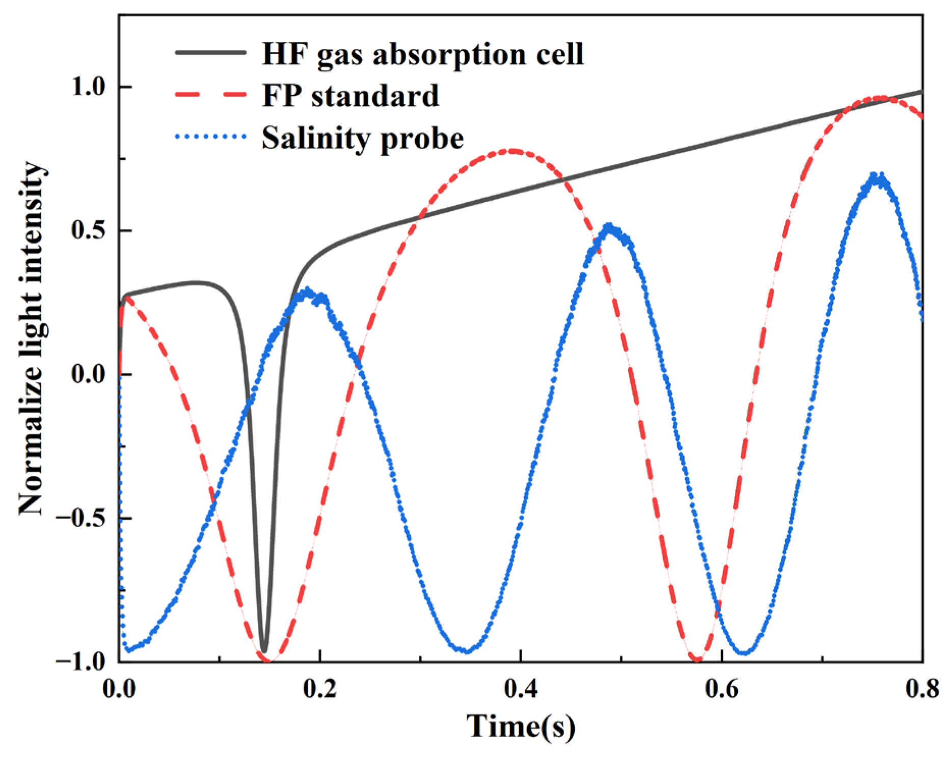
3.2.2. Mathematical Models

Despite the complexity of salinity in the shallow sea, the initial stages of the sea entry were challenging due to the uncontrolled descent speed and significant stirring of the seawater. These issues could potentially result in inconsistencies in the water characteristics measured by the optical salinity probe and SBE 37, preventing the completion of high-precision comparative measurements. The temperature, depth, and salinity measurement results from SBE37 are depicted in Figure 8a–c, respectively. The salinity sensor begins descending uniformly at a rate of approximately 1.1 m/s at a depth exceeding 200 m. Notably, within the descending depth range from 200 to 1500 m, which includes the thermocline of the seawater, the temperature rapidly decreases from 20 °C to 3 °C. Subsequently, between 1500 and 4000 m, the temperature change of the seawater tends to vary very slowly. During the profiling test conducted at various ocean depths, as shown in Figure 8c, the salinity exhibits a pattern of first decreasing and then increasing when passing through the intermediate water layer at depths of 200–1000 m. The primary reason for this phenomenon is that the intermediate water in the South China Sea primarily originates from the North Pacific Intermediate Water (NPIW) masses, which are formed at mid to high latitudes in the North Pacific. These water masses can spread and enter the South China Sea during colder periods. Since NPIW naturally has lower salinity, its intrusion directly causes a decrease in the salinity of the intermediate waters in the South China Sea [29,30].

This RI is a complex function influenced by temperature, salinity, and depth [31]. In this study, the M-S equation was deployed to establish the mathematical relationship between the sensor’s original output value (ΔZ) and oceanic parameters: temperature (T), salinity (S), and depth (P). To determine the coefficients of this equation, the nonlinear least squares fitting method was utilized, resulting in the derivation of Equation (6). Equation (2) is applicable to depths ranging from 200 to 4000 m. As depicted in Figure 8d, the sensor’s original output (ΔZ) closely aligns with the fitted results based on temperature, salinity, and depth, with a maximum error of less than 0.12%. Salinity measurements were obtained by solving the inverse function of Equation (6). The results of salinity calculations are shown in Figure 8e. It is evident that the optical salinity sensor demonstrated superior tracking performance. Notably, the maximum salinity demodulation error occurred within the thermocline layer, amounting to 0.005 psu.

$$\begin{array}{l}\Delta Z=a_1\cdot T+a_2\cdot T^2+a_3\cdot T^3+a_4\cdot T^4+a_5\cdot T\cdot \lambda +a_6\cdot T^2\cdot \lambda +a_7\cdot \lambda \cdot T^3+a_8\cdot S\\ +a_9\cdot S/{\lambda }^2+a_{10}\cdot S\cdot T+a_{11}\cdot S\cdot T^2+a_{12}\cdot S\cdot T^3+a_{13}\cdot S\cdot T\cdot \lambda +a_{14}\cdot P+a_{15}\cdot P^2\\ +a_{16}\cdot P/{\lambda }^2+a_{17}\cdot P\cdot T+a_{18}\cdot P\cdot T^2+a_{19}\cdot P^2\cdot T^2+a_{20}\cdot P\cdot S+a_{21}\cdot P\cdot S\cdot T\end{array}$$

(6)

The observed error is primarily attributed to two key factors. Firstly, salinity errors might arise from the asynchronous timing of temperature and conductivity measurements performed by the SBE37 during its fast descent through the thermocline [10]. Secondly, the position difference between the optical salinity sensor and SBE 37 on the brackets led to a temperature difference of about 3–4 mK during the descending process, which could lead to a fitting bias of optical salinity sensor about 0.002 psu. As the depth exceeded 1500 m, the demodulation error decreased significantly to be less than 0.0005 psu, indicating a remarkable level of sensing accuracy.

4. Experiment Results and Discussion

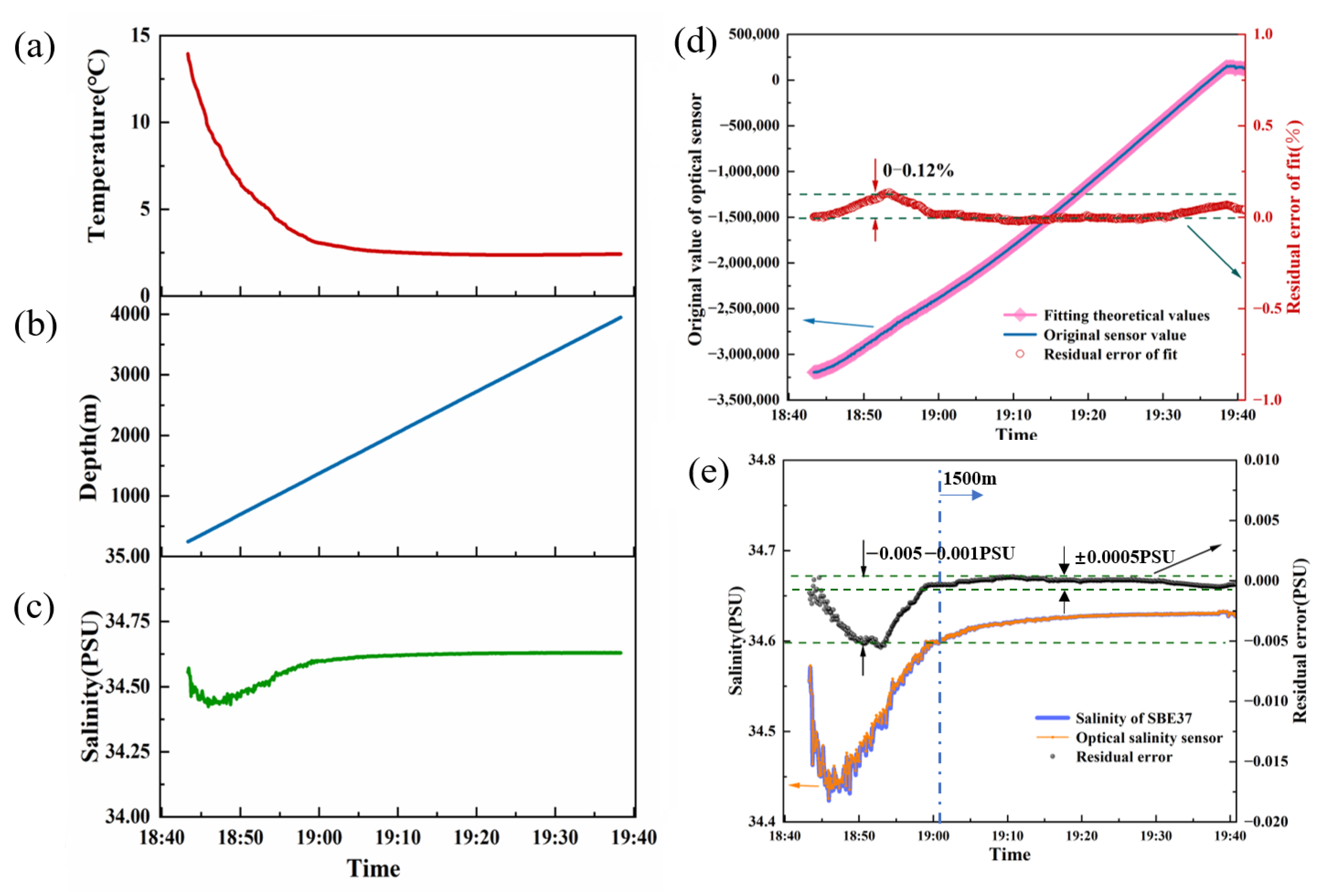
4.1. In Situ Sensing Ability of Salinity in Profiles

During the descending ocean profiling in the South China Sea, data were collected by SBE 37 and utilized as a fitting reference to calibrate and fit the optical salinity sensor. This approach established a relationship between salinity, temperature, pressure, and the sensor’s original output. Ten hours later, the sensors were ascending from the bottom of the ocean, and the data collected during the upwelling process were used to assess the performance of the optical salinity sensor. Though optical temperature and pressure sensors were also integrated with this optical salinity sensor and included in the same titanium tank during this sea trial, and obtained good results in comparison with those of SBE 37, in this work, the temperature and pressure data from SBE 37 were used instead of those of the optical data, for the consideration of consistency with the calibration result obtained from the descending data.

The temperature, salinity, and pressure profiles of the SBE 37 during the ascending process are depicted in Figure 9a–c, respectively. In Figure 9c, it is noteworthy that the optical salinity sensor demonstrates a high degree of consistency with the results obtained from the SBE37. This correlation indicates the good accuracy of the optic salinity sensor after calibration by SBE37 using the data of the descending process. As the sensors traversed the thermocline layer, the drastic temperature change resulted in a discrepancy of 0.005 psu between the optical salinity sensor and SBE 37. The percentage of differences between the optical salinity sensor and the SBE 37 in the range of ±0.002 psu during the upswing is about 95%.

4.2. In Situ Deep-Sea Salinity Sensing

The salinity versus time curves of the optic salinity sensor and SBE37 obtained during the ten-hour seabed exploration are depicted in Figure 10a. The overlap between the two datasets is excellent, with a fitting error of less than ±0.0005 psu, indicating a high degree of agreement and the reliability of both measurement systems. In order to further evaluate the performance of the salinity sensor, ten hours of stability data were analyzed for Allan deviation. The lowest point of Allan’s deviation occurred after 25 min, with a salinity resolution of 1.89 × 10⁻⁵ psu, as shown in Figure 10b.

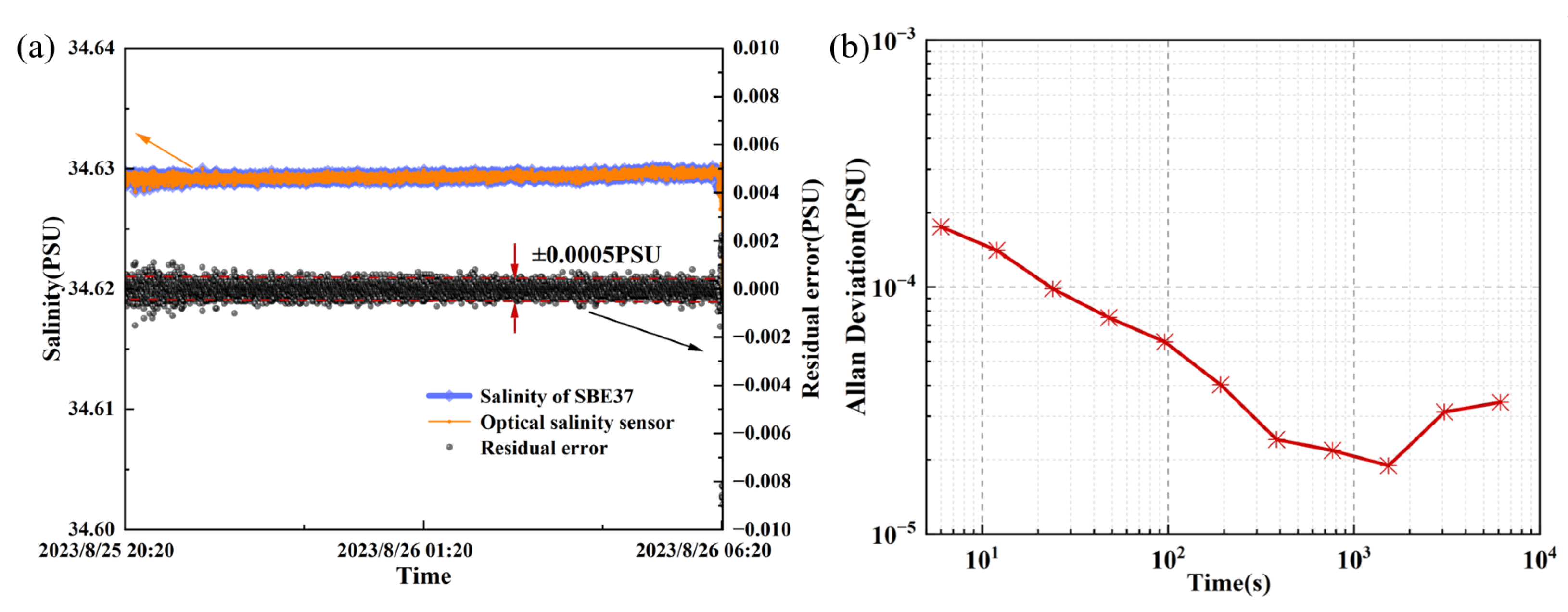
4.3. In Situ Long-Term Salinity Sensing

After the descending and ascending profiling tests were completed, the optic salinity sensor and SBE37 were dropped into the deep sea (4000 m) for a three-month long-term deployment. For the sake of power saving, the optical salinity sensor was set to operate five minutes every three hours at a sampling frequency of 0.5 Hz for the three-month period. Meanwhile, the SBE 37 was configured to sample every 10 min for uninterrupted operation. The average of the 5 min measurements from the original optical system data was used as the initial value for the optical salinity sensor. Temperature and depth data were similarly taken at 3 h intervals, selected from SBE37 data from a time period close to the optical sensor tests. Figure 11 depicts the salinity data measured by the optical salinity sensor and SBE37, as well as their discrepancy, which is within ±0.002 psu. In a comparison of the salinity sensing data between the first and last day of testing, as shown in

Table 2. Percentage of error.

	Salinity of SBE37/Psu	Salinity of the Sensor/Psu	Error/Psu	Percentage of Error
First day	34.6003	34.59947	8.35957 × 10−4	0.00242%
Last day	34.600013	34.59936	7.6885 × 10−4	0.00222%

, the salinity errors are 8.35957 × 10⁻⁴ psu and 7.6885 × 10⁻⁴ psu, respectively. The difference is 6.7107 × 10⁻⁵ psu, which is a good demonstration of the stability of the salinity sensor during three months of seabed testing. This result confirms the accuracy and stability of the optic salinity sensor in deep-sea operation.

4.4. Comparison and Analysis

Table 3. Performance comparison of salinity sensors based on different principles.

Sensing Principle	Core Component	Resolution /Psu	Advantages and Disadvantages
Electrical conductivity [SBE37]	Conductivity cell	0.002	Broadly applied in ocean observation, but ignores non-conductive substances in seawater
Total internal reflection [21]	CCD	0.05	Compact structure, but only suitable for surface seawater measurement with low resolution
V-block refraction [22]	PSD	0.001	Simple structure and small size, but not suitable for deep sea
Optical interferometer [13]	Thickness meter	0.00015	High resolution, but complex demodulation system, lack of structural stability in deep sea
Michelson interferometer	FMCW	0.0000189	High resolution, simple modulation system, long-term stability in deep sea

compares salinity sensors based on different principles. Conductivity-based salinity sensors, represented by the SBE37, have been widely used in marine research for two decades. They measured seawater salinity based on the contribution of the conductive substance in seawater, but ignored the contribution of non-conductive substances. RI-based salinity measurement was either low-resolution or not suitable for deep-sea application in a high-pressure environment. Previously reported salinity sensors based on optical interferometers have the advantage of high sensitivity, but may require additional temperature compensation due to the use of hetero-media with different thermal optical coefficients in the two interference arms. The optical Michelson interferometer salinometer proposed in this article not only has high resolution, but also has a symmetrical interference arm that has demonstrated long-term stability in seabed tests.

5. Conclusions

An optical salinometer based on a Michelson interferometer is proposed and experimentally demonstrated in a deep-sea environment in this work. The optic salinity sensor is based on an FMCW-modulated DFB laser with a wavelength of 1260 nm, deploying an HF gas absorption peak for in situ calibration of the laser wavelength drift in real time and using a cross-correlation demodulation algorithm. After an FEM simulation, the feasibility of the optical structure was verified. The optic salinity sensor was calibrated and tested at the location with a depth of 4000 m in the South China Sea. The optic salinity sensor was calibrated by SBE37 during the descending process from 200 to 4000 m in depth. After calibration, the optic salinity sensor was examined by comparison with SBE 37 during the ascending process from 4000 m depth to the sea surface, with ten-hour and three-month seafloor (4000 m) deployments. It has been demonstrated that the optical salinity sensor has a resolution of 1.89 × 10⁻⁵ psu and an accuracy of ±0.002 psu during a three-month comparison with SBE37.

References

1. Gu, L.; He, X.; Zhang, M.; Lu, H. Advances in the technologies for marine salinity measurement. J. Mar. Sci. Eng. 2024, 10, 2024. [Google Scholar] [CrossRef]
2. Li, G.; Cheng, L.; Zhu, J.; Trenberth, K.E.; Mann, M.E.; Abraham, J.P. Increasing ocean stratification over the past half-century. Nat. Clim. Change 2020, 10, 1116–1123. [Google Scholar] [CrossRef]
3. Evans, T.G.; Kültz, D. The cellular stress response in fish exposed to salinity fluctuations. J. Exp. Zool. Part A 2020, 333, 421–435. [Google Scholar] [CrossRef]
4. Forch, C.; Knudson, M.; Sorensen, S. Reports on the determination of the constants for compilation of hydrographic tables. Det K. Dan. Vidensk. Selsk. Skrifter. Naturvidenskabelig Og Math. Afd. 1902, 6, 1–151. [Google Scholar]
5. Lewis, E. The practical salinity scale 1978 and its antecedents. IEEE J. Ocean. Eng. 1980, 5, 3–8. [Google Scholar] [CrossRef]
6. IOC; SCOR; IAPSO. The International Thermodynamic Equation of Seawater-2010: Calculation and Use of Thermodynamic Properties; Intergovernmental Oceanographic Commission: Paris, France, 2010. [Google Scholar]
7. Millero, F.J.; Feistel, R.; Wright, D.G.; McDougall, T.J. The composition of standard seawater and the definition of the reference-composition salinity scale. Deep-Sea Res. Pt. I 2008, 55, 50–72. [Google Scholar] [CrossRef]
8. Mcdougall, T.J.; Jackett, D.R.; Millero, F.J.; Pawlowicz, R.; Barker, P.M. A global algorithm for estimating Absolute Salinity. Ocean. Sci. 2012, 8, 1123–1134. [Google Scholar] [CrossRef]
9. Zhang, C.; Xiao, Y.; Gao, W.; Fu, Y.; Zhou, Z.; Chen, S.; Su, J.; Wu, C.; Wu, A. Contribution of dissolved organic matter to seawater salinity measured by optic refractometer: A case study of DOM extracted from aoshan bay. Front. Mar. Sci. 2023, 10, 1142718. [Google Scholar] [CrossRef]
10. Su, J.; Xiao, Y.; Chen, S.; Zhang, C.; Gao, W.; Fu, Y.; Bai, X.; Wu, C. Comparison of Salinity Measurement Based on Optical Refractometer and Electric Conductivity: A Case Study of Urea in Seawater. IEEE Sens. J. 2024, 24, 2172–2179. [Google Scholar] [CrossRef]
11. Millard, R.C.; Seaver, G. An index of refraction algorithm for seawater over temperature, pressure, salinity, density, and wavelength. Deep-Sea Res. Pt. A 1990, 37, 1909–1926. [Google Scholar] [CrossRef]
12. Wang, X.; Bai, X.; Zhang, M. Optical salinity sensing based on Michaelson interferometer under water pressure up to 11,500 meters. Ocean Eng. 2024, 299, 117307. [Google Scholar] [CrossRef]
13. Uchida, H.; Kayukawa, Y.; Maeda, Y. Ultra high-resolution seawater density sensor based on a refractive index measurement using the spectroscopic interference method. Sci. Rep. 2019, 9, 15482. [Google Scholar] [CrossRef] [PubMed]
14. Held, P.; Kegler, P.; Schrottke, K. Influence of suspended particulate matter on salinity measurements. Cont. Shelf Res. 2014, 85, 1–8. [Google Scholar] [CrossRef]
15. Friedman, A.R.; Reverdin, G.; Khodri, M.; Gastineau, G. A new record of Atlantic sea surface salinity from 1896 to 2013 reveals the signatures of climate variability and long-term trends. Geophys. Res. Lett. 2017, 44, 1866–1876. [Google Scholar] [CrossRef]
16. Tian, P.; Zhu, Z.; Wang, M.; Ye, P.; Yang, J.; Shi, J.; Yang, J.; Guan, C.; Yuan, L. Refractive Index Sensor Based on Fiber Bragg Grating in Hollow Suspended-Core Fiber. IEEE Sens. J. 2019, 19, 11961–11964. [Google Scholar] [CrossRef]
17. Zhang, X.; Peng, W. Temperature-Independent Fiber Salinity Sensor Based on Fabry-Perot Interference. Opt. Express 2015, 23, 10353–10358. [Google Scholar] [CrossRef]
18. Lin, Z.; Lv, R.; Zhao, Y.; Zheng, H.; Wang, X. High-Sensitivity Special Open-Cavity Mach-Zehnder Structure for Salinity Measurement Based on Etched Double-Side Hole Fiber. Opt. Lett. 2021, 46, 2714–2717. [Google Scholar] [CrossRef]
19. Zhao, Y.; Zhao, J.; Wang, X.; Peng, Y.; Hu, X. Femtosecond Laser-Inscribed Fiber-Optic Sensor for Seawater Salinity and Temperature Measurements. Sens. Actuators B Chem. 2022, 353, 131134. [Google Scholar] [CrossRef]
20. Wang, X.; Wang, J.; Wang, S.; Liao, Y. Fiber-optic salinity sensing with a panda-microfiber-based multimode interferometer. J. Light. Technol. 2017, 35, 5086–5091. [Google Scholar] [CrossRef]
21. Chen, J.; Guo, W.; Xia, M.; Li, W.; Yang, K. In situ measurement of seawater salinity with an optical refractometer based on total internal reflection method. Opt. Express 2018, 26, 25510–25523. [Google Scholar] [CrossRef]
22. Malardé, D.; Wu, Z.Y.; Grosso, P.; de la Tocnaye, J.-L.d.B.; Le Menn, M. High-resolution and compact refractometer for salinity measurements. Meas. Sci. Technol. 2009, 20, 015204. [Google Scholar] [CrossRef]
23. Menn, M.L.; de la Tocnaye, J.-L.d.B.; Grosso, P.; Delauney, L.; Podeur, C.; Brault, P.; Guillerme, O. Advances in measuring ocean salinity with an optical sensor. Meas. Sci. Technol. 2011, 22, 115202. [Google Scholar] [CrossRef]
24. Li, G.; Li, G.; Yang, S.; Ji, L.; Sun, Q.; Su, J.; Wu, C. A novel salinity sensor with high-resolution and large dynamic range based on optical Fabry-Pérot cavity. Sens. Actuator A Phys. 2022, 347, 113970. [Google Scholar] [CrossRef]
25. Li, G.; Yang, S.; Wu, C. Seeing more clearly: Improving the resolution of ocean salinity measurements using a Fabry-Perot resonant cavity. Opt. Laser Eng. 2024, 181, 108356. [Google Scholar] [CrossRef]
26. Yang, S.; Ji, L.; Zhao, S.; Sun, Q.; Xu, J.; Wu, C. High-resolution Michelson Salinometer Based on Frequency-modulated Continuous-wave Interferometry. IEEE Sens. J. 2024. early access. [Google Scholar] [CrossRef]
27. Ji, L.; Zhao, S.; Sun, Q.; Yang, S.; Bai, X.; Zhao, P.; Su, J.; Wu, C. Seawater Temperature Measurement System Based on Wavelength Sweeping and Cross Correlation Algorithm. IEEE Sens. J. 2023, 23, 9280–9286. [Google Scholar] [CrossRef]
28. Ji, L.; Sun, Q.; Zhao, S.; Sun, Q.; Yang, S.; Bai, X.; Zhao, P.; Su, J.; Wu, C. High-resolution fiber grating pressure sensor with in-situ calibration for deep sea exploration. Opt. Express 2023, 31, 10358–10367. [Google Scholar] [CrossRef]
29. Qu, T.D.; Mitsudera, H.; Yamagata, T. Intrusion of the North Pacific waters into the South China Sea. J. Geophys. Res.-Oceans 2000, 105, 6415–6424. [Google Scholar] [CrossRef]
30. You, Y.Z.; Chern, C.S.; Yang, Y.; Liu, C.-T.; Liu, K.-K.; Pai, S.-C. The South China Sea, a cul-de-sac of North Pacific intermediate water. J. Oceanogr. 2005, 61, 509–527. [Google Scholar] [CrossRef]
31. Quan, X.; Fry, E.S. Empirical equation for the index of refraction of seawater. Appl. Opt. 1995, 34, 3477–3480. [Google Scholar] [CrossRef]
Figure 1. Schematic structure of the MI optical salinometer. (a) Three-dimensional appearance of the probe; (b) optical path, sapphire optical window, and titanium tank; (c) schematic of the physical length of the optical path of the probe.
Jmse 12 01569 g001
Figure 2. Side view of sapphire placement.
Jmse 12 01569 g002
Figure 3. (a) Simulation; (b) deformation of sapphire under pressure.
Jmse 12 01569 g003
Figure 4. (a) Flow field distribution during the descent of an optical pressure-resistant probe in seawater at a speed of 1.5 m/s; (b) flow field distribution in the flow channel at different velocities and angles.
Jmse 12 01569 g004
Figure 5. Schematic of the FMCW-based MI salinity sensing system, (a) the optical path of the optical sensor, and (b) the internal wiring of the titanium tank of the optical sensor.
Jmse 12 01569 g005
Figure 6. The black solid line represents the signal obtained from the HF gas absorption cell; the red dashed line depicts the signal from the FP standard fixture; the blue dotted line corresponds to the signal from the optical salinity sensor.
Jmse 12 01569 g006
Figure 7. Titanium tanks and optical pressure-resistant probes and their mounting brackets.
Jmse 12 01569 g007
Figure 8. Optical salinity sensor descending process and curve fitting. (a) Temperature change curve of SBE37 during the sea trial. (b) Depth change curve of SBE37 during the sea trial. (c) Salinity change curve of SBE37 during the sea trial. (d) Fitting of the mathematical relationship between the sensor’s original output value (ΔZ) and oceanic parameters: temperature (T), salinity (S), and depth (P), and the residual error. (e) Measured salinities from the optical salinity sensor and SBE37 during the descending process in the sea trial.
Jmse 12 01569 g008
Figure 9. Measured temperature, salinity, and depth during the ascending process from the seafloor (4000 m) to the sea surface by the optical salinity sensor and SBE 37. (a) Measured temperature from SBE37 during the ascending process in the sea trial. (b) Measured depth from SBE37 during the ascending process in the sea trial. (c) Measured salinities from the optical salinity sensor and SBE37 during the ascending process in the sea trial.
Jmse 12 01569 g009
Figure 10. (a) Ten-hour deep-sea (4000 m) measurement by optic salinity sensor and SBE 37 and (b) Allan deviation.
Jmse 12 01569 g010
Figure 11. A three-month comparison test between the optic salinity sensor and SBE 37 at the seafloor depth of 4000 m.
Jmse 12 01569 g011