A New Insight on the Upwelling along the Atlantic Iberian Coasts and Warm Water Outflow in the Gulf of Cadiz from Multiscale Ultrahigh Resolution Sea Surface Temperature Imagery

Abstract

The ATLAZUL project is an Interreg effort among 18 partners from Spain and Portugal along the Atlantic Iberian coasts. One of its objectives is the development of new methods and data processing for oceanic information to produce useful products for private and public stakeholders. This study proposes a new insight on the sea surface dynamic of the ATLAZUL area based on almost two years of multiscale high resolution sea surface temperature imagery. The use of techniques such as the Karhunen–Loève transform (Empirical Orthogonal Function) and the Maximum Entropy Spectral Analysis were applied to study long- and short-term features in the sea surface temperature imagery. Mathematical Morphology and the Geometrical Theory of Measure are utilized to compute the Medial Axis Transform and the Hausdorff dimension. The results can be summarized as follows: (i) the tow upwelling areas are identified along the Galician–Portugal coast as indicated in the second and third modes of KLT/EOF analysis, and they are partially affected by wind; (ii) the tow warm water outflows from the Bay of Cádiz to the Gulf of Cádiz are identified as the second and third modes of KLT/EOF analysis, which are also influenced by wind; (iii) the skeletons of the surface signature of the upwelling and of the warmer water outflow, along with their fractal dimensions, indicate a chaotic pattern of spatial distribution and (iv) the harmonic prediction model should be combined with the wind prediction.

1. Introduction

ATLAZUL is an Interreg strategic project sponsored by the Junta de Andalucía (Spain) under the first objective of the POCTEP program for the Research + Development + Innovation (see atlazul.eu). One of its objectives is the production of useful information for public and private actors. The ATLAZUL area encompasses the coasts of Galicia (Spain), Portugal and the Gulf of Cádiz (Figure 1). Fishermen’s guilds operating in this region are closely related to the sea surface temperature (SST) as well as City Halls with interest in the coastal zone need for practical products for the management of their activities. This study focuses on examining the variability of the SST field in the ATLAZUL area through the modal decomposition of nearly two years of satellite imagery. Additionally, the feasibility of the long-term harmonic SST prediction model is examined.

SST is the most useful physical parameter for monitoring the occurrence of upwelling and downwelling areas, especially from privileged observational platforms such as artificial satellites. It is well known that the seawater temperature acts as a climate regulator. Because nearly all artificial satellite missions include an SST sensor, space agencies have developed multi-mission products, such as those from the Jet Propulsion Laboratory (JPL). We have used the Multiscale Ultrahigh Resolution Sea Surface Temperature (MUR-SST) dataset. This work takes advantage of the RAIA observatory (https://marnaraia.org, accessed on 5 December 2023) to obtain the wind speed and direction data from the most western station in the Galician coasts, the Boia da Ribeira (Figure 1), and the meteorological station at the Observatorio del Parque Natural Bahía de Cádiz at the Gulf of Cádiz (Figure 1).

The ATLAZUL area has been studied from many perspectives. The plumes and filaments from the upwelling along the Galician and Portuguese coasts were studied highlighting a seasonal behavior [1]. The coastal current system along the Portuguese coasts from a chemical standpoint, as well as its coupling with the upwelling, are detailed in [2]. The use of drifters and altimetry to study the dynamic of the area was carried out in [3]. A review of the oceanic circulation focusing on fronts, eddies and poleward currents can be found in [4]. A more focused review on the marine ecology, relating oceanography and fisheries within the Canary Current and along the Portuguese coasts, is available in [5]. An overview, with many open questions, on the relationship among the processes occurring on the continental shelf, coastal currents, eddies, plumes upwelling, fronts and internal waves in the area can be found in [6]. The common theme in [1,2,3,4,5,6] is that the signature of the cooler waters along the Galician and Portugal coasts exhibits a strong seasonal component. However, the connections between the open sea and the coastal domain, influenced by eddies and coastally trapped waves, are only considered in [6]. Regarding the Gulf of Cádiz, the seasonal and interannual evolution of the surface current between San Vicente Cape and the Strait of Gibraltar, based on a short time series of SST, is the focus in [7], which details the influence of the outflow of the Strait of Gibraltar but not the warmer outflow from the Bay of Cádiz. A complete numerical modeling covering the entire ATLAZUL area, describing the surface currents and reinforcing the seasonal character of the oceanographic phenomena is conducted in [8]. While upwelling along the Galician–Portugal coasts is addressed, there is no mention to the warmer water outflow from the Bay of Cádiz. The influence of the SST, salinity, river discharges, mean sea level and tides on the estuaries along the coasts of the ATLAZUL area is examined in [9]. These works have several common points: they indicate that this is a very complex area with a strong driving seasonal force [1,2,3,4,5,6,7,8], highlight the large variations of the SST in the Galician–Portugal coasts [1,2,3,4,5,6] and emphasize the importance of the inflow–outflow at the Strait of Gibraltar [6,7,8]. However, they overlook the significant warm water outflow from the Bay of Cádiz. This study focuses on the upwelling in the Galician–Portugal coasts and the warmer water outflow in the Gulf of Cádiz.

The study of complex phenomenon, such as the spatiotemporal structure of upwelling from its SST signature, can be simplified using the Karhunen–Loève transform (KLT) [10,11,12,13]. The KLT is a numerical technique close to the Hotelling transform [14], which is known in Physical Oceanography as the Empirical Orthogonal Function [15], with a proper data structure [16,17]. This leads to two main results: the spectrum of the problem and a set of separable spatiotemporal modes in a double-linked basis of spatial and temporal modes. The spectrum of the problem facilitates the selection of the number of modes necessary to explain or reconstruct the phenomenon without the noisier modes or to isolate a given feature. The spatial modes, or spatial weights, give the distribution of the importance of each mode at individual points. Conversely, the temporal modes, or temporal weights, reveal the temporal evolution of each paired spatial mode. These modes can be utilized for harmonic prediction, with maximum entropy spectral analysis as the best option for the estimation of the power spectral density [11,18]. The application of the KLT/EOF approach will allow the definition of nodal lines and the clustering of areas [10,11,12,13].

On the other hand, the digital image processing suffered a major change with the development of the Mathematical Morphology [19,20,21,22]. The use of the morphological operators led to a more effective denoising, as the closing operator, and feature extraction from digital images. The Medial Axis Transform (MAT) reduces the objects to a one-pixel-thick geometrical structure occupying the same place and keeping the dimensions, the skeleton. The way of filling the space of such a new geometrical structure is resumed in the fractal or Hausdorff dimension, D₀. The combination of Mathematical Morphology and the Geometric Theory of the Measure is a very powerful tool to delve deep into the internal organization of the spatial structure [10,11,12,13].

This study focuses on two key regions: the Galician and Portugal coasts and the Gulf of Cádiz. From the combination of physical–mathematical tools—the KLT/EOF, the Maximum Entropy Spectral Analysis, the least squares harmonic prediction, the Medial Axis Transform and the fractal dimension—this work aims to enhance the knowledge of the ATLAZUL area. The goal is to produce valuable products for the different public and private stakeholders such as researchers, universities, governmental offices, city halls and fishermen’s guilds in the area to assist their planning activities.

Our findings indicate that the entire ATLAZUL domain exhibits a strong seasonal component with a highly variable sea surface temperature (SST) along the Galician and Portuguese coasts. The warmer water outflow from the Bay of Cádiz occurs in the summer due to intense solar heating in the region, representing a secondary seasonal phenomenon. The wind influences oceanographic processes significantly, but its effects are episodic, thereby reinforcing other oceanographic phenomena. We also propose that a harmonic prediction model for SST fields in both areas would be beneficial for the planning activities of fishermen’s guilds and other public and private stakeholders.

The organization of this article is as follows: Section 2 is devoted to describing the area, the data and the physical–mathematical tools used in the frame of this study. Results and discussion are combined in Section 3. Finally, conclusions are drawn in Section 4.

2. Materials and Methods

2.1. Satellite Imagery

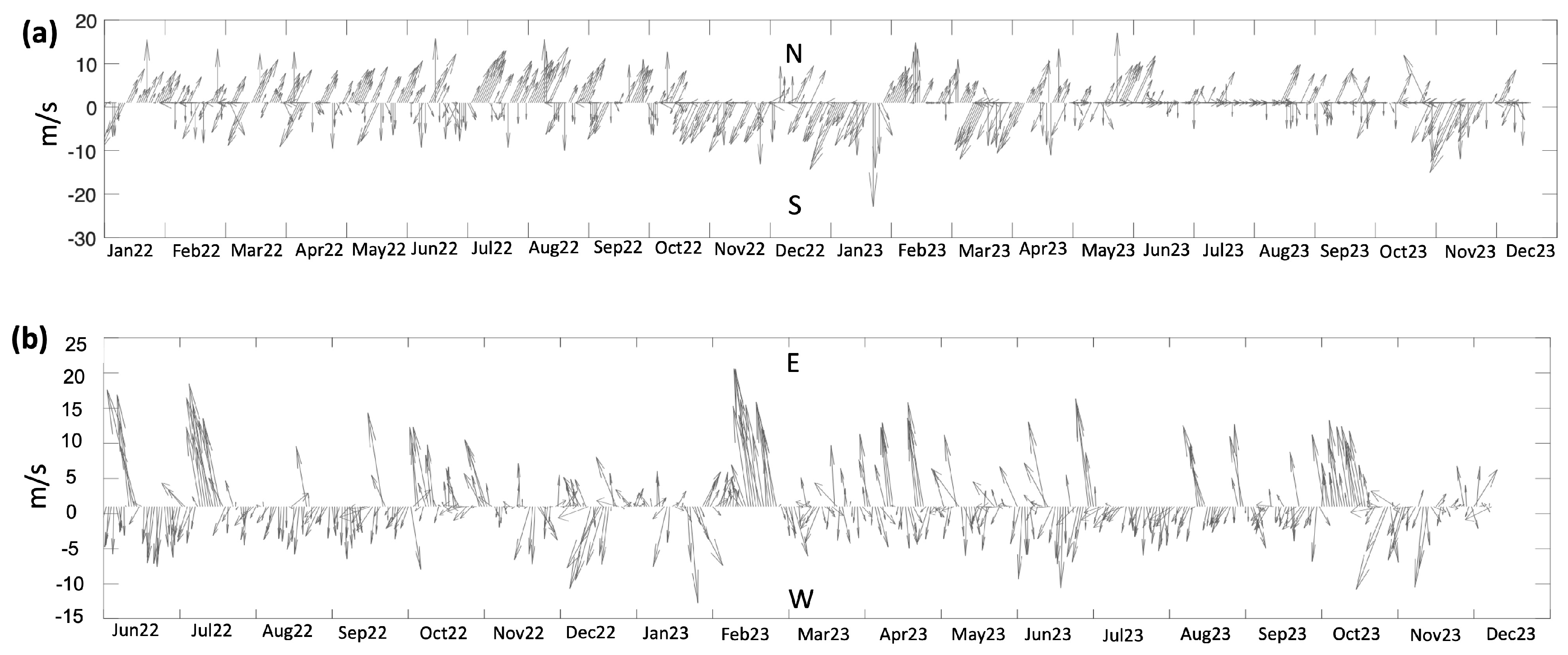
The Multiscale Ultrahigh Resolution imagery for Sea Surface Temperature (MUR-SST) is produced at the Jet Propulsion Laboratory (Pasadena, CA, USA). MUR-SST is a product consisting of daily global SST fields represented on a 0.01° grid with an equatorial spatial resolution of 1.1132 km. The product integrates data from multiple satellite missions with different resolutions over different time scales, combined using multiresolution variational analysis on a specified wavelet basis. MUR-SST combines the SST data from Aqua/MODIS, Aqua/AMSR-E, CORIOLIS/WINDSAT, Terra/MODIS, NOAA-19/AVHRR-3 and GCOM-W1/AMSR2 missions as well as in situ datasets [23]. We take advantage of the daily imagery spanning from 1 January 2022 to 30 November 2023, in two segments. The training segment comprises 638 fields up to 30 September 2023, and October and November 2023 are the second segment, devoted to validating the results.

2.2. Wind Data

Two mean daily wind data time series have been used in the frame of this study. The first one is sourced from the RAIA observatory (https://marnaraia.org). The Boia de Ribeira dataset, in La Coruña at coordinates (−8°56.87′ W, 42°32.98 ′N) (Figure 1), spans from 1 January 2022 to 30 November 2023. The second one, from the Observatorio Ambiental del Parque Natural Bahía de Cádiz (https://widgets.ocean.uca.es/meteodata/, accessed on 5 December 2023), in Cádiz at coordinates (36.5300° N, 6.2120° W) (Figure 1) covers from 1 June 2022 to 30 November 2023.

2.3. The Karhunen–Loève Discret Transform or EOF on Digital Imagery

According to [17,18], the general class of transformations known as Principal Component Analysis (PCA) is referred to as Hotelling’s transform [14]. A special case of Hotelling’s transform is the Karhunen–Loève Discrete Transform (KLT), which was independently proposed by [24,25]. In Physical Oceanography, the KLT is commonly known as the Empirical Orthogonal Function Decomposition (EOF) [16]. The KLT/EOF is applied to a two-dimensional scalar field time series, such as digital images, and decomposes it onto a double empirical linked basis: one comprises two-dimensional spatial modes, or weights, and the other consists of time series for temporal weights. The KLT/EOF has been extensively applied for reducing the complexity of digital images [26], de-noising and facial pattern recognition [27,28,29] and feature extraction [16]. One of the first application of the KLT/EOF on satellite SST imagery to study upwellings was in [10,11,12,13].

In the context of digital image processing for feature extraction, a single scene is referred as “snapshot”, $\mathsf{\Phi }(\underset{\_}{x},t_n)$, where x represents the position vector and t_n is a specific time. The ensemble of the snapshots, $\mathsf{\Phi }\left(\underset{\_}{x},t\right)=\{\mathsf{\Phi }\left(\underset{\_}{x},t_n\right){\}}_{n=1,m}$, is the super-snapshot. The mean field, $\overline{\mathsf{\Phi }}\left(\underset{\_}{x}\right)$, is subtracted before decomposing, so the time series is now the SST anomaly. A snapshot, $\mathsf{\Phi }(\underset{\_}{x},t_n)$, is decomposed onto a sum of m separable products of temporal functions, $\left\{A_i\right(t\left)\right\}$, and spatial modes, $\left\{{\mathsf{\Psi }}_i\right(\underset{\_}{x}\left)\right\}$, with i = 1, m. Each corresponding singular value, M_i, reflects the importance of each mode:

$$\mathsf{\Phi }\left(\underset{\_}{x},t_n\right)={\sum }_i{M}_i{A}_i\left(t_n\right){\mathsf{\Psi }}_i\left(\underset{\_}{x}\right)$$

(1)

The numerical version in terms of the eigenvalue problem is as follows:

$${\lambda }_i{A}_i\left(t\right)={\sum }_{t^{’}}{C}_{t{t}^{’}}{A}_i(t’)$$

(2)

where ${\lambda }_i$ is the i-th eigenvalue and C_tt’ is the covariance matrix for the snapshots. Once the temporal modes are estimated from Equation (2) the i-th spatial mode is given by [30,31]:

$${\mathsf{\Psi }}_i\left(\underset{\_}{x}\right)=M_i{A}_i\left(t\right)\mathsf{\Phi }(\underset{\_}{x},t)$$

(3)

The importance of each mode in terms of the percentage of the explained variance is computed by means of

$${Importance}_i\left(\mathrm{\%}\right)={\displaystyle \frac{{\lambda }_i^2}{\sum {\lambda }_i^2}}·100$$

(4)

The results of the KLT/EOF decomposition include the mean field, the importance of each mode, and both the spatial and temporal modes. The spectrum of the problem indicates how many modes must be considered to explain a percentage of the variance up to the scientist’s discretion. For further details on the application of the KLT on satellite SST imagery, the reader is referred to previous works [11,12,13,14].

2.4. Mathematical Morphology and the Geometric Theory of the Measure

Mathematical Morphology is a physical theory that considers the elements of a digital image as sets and subsets embedded into a topological space. The connectivity of the different elements is the most important feature to apply the morphological operators. The basic operations are the same as in the Theory of Sets [19,20] grouped in morphological operators for digital image processing as noise elimination [32], segmentation (opening, closing, erosion and dilation) [19,20,21,22], contrast enhancing [19,20,32,33] and much more.

The only morphological operator used in this study is a closing operator. Following [19,20,21,22], the closing operator involves the fundamental morphological actions of dilation and erosion. Dilation consists of filling the small background holes in the image, distorting it. Erosion eliminates the undesirable effect of the dilation. Then, the closing operator is a dilation followed by erosion. Its dual operator is the opening: an erosion followed by a dilation, being not commutative. The closing morphological operator reduces the alternating and disperses black and white pixels known as salt and pepper, or impulse, noise. In addition, it smooths very small structures.

Computing the skeleton of any geometrical object is intuitive but not easy. The skeleton is a one-pixel thick geometrical object in the axis of the object and preserves its topology. The skeleton can be computed from several algorithms. The only conditions are that they must preserve place, connectivity and size. It is possible to apply a recursive thinning with a differential treatment to those pixels at the end of the object and to erode only one pixel each time. The process reduces the foreground regions to a skeletal structure, preserving the size and connectivity of the original region. This is known as Medial Axis Transformation or MAT [21,22,34,35].

The recipe to get the skeleton can be as follows. After the proper binarization of the image or object to compute the skeleton, a structural element is defined (i.e., a square of three pixels per side). Then, there is a dilation followed by an erosion, the closing operator, is applied, convoluting it by means of the structural element. Finally, the skeleton is recovered, invoking the black and white morphology and using the structural element. This step requires iterations. The higher the number of iterations, the better quality in the skeleton and the longer the CPU time. However, once the skeleton is obtained, additional iterations have no effect on it [13]. We have applied 300 iterations for the purposes of automation to ensure a high quality skeleton extraction.

The ideal travel companion for the MAT at the time of characterizing a geometrical object is the Geometric Theory of the Measure [10,11,12,13]. Measuring a set by covering it with an already known measure set, say a ε-blanket, leads to the fractal dimension. The covering element of the ε-blanket can have any suitable form, say squares with different sizes. The computation of the fractal or Hausdorff dimension is not easy but if the size of the covering set is small enough, the fractal dimension and the box counting dimension coincide. This is written as follows [34,35]:

$$D_0=\underset{\epsilon \to 0}{\lim }{\displaystyle \frac{\mathrm{l}\mathrm{o}\mathrm{g}\left(N\right(\epsilon \left)\right)}{\mathrm{l}\mathrm{o}\mathrm{g}\left(\epsilon \right)}}$$

(5)

where ε is the length of the ε-blanket elements and N(ε) is the number of elements needed to cover the object. D₀ is the dimension. Keeping the domain, the fractal dimension is unsensitive under rotation and translation. Some applications of the Mathematical Morphology and Geometrical Theory of the Measure can be found in [10,11,12,13]. Some explanation is needed to compute Equation (5). The plot of log(ε) with log(N(ε)) has three regions: a region corresponding to low values of ε, which has no information, an intermediate area named the scaling region and a flat ending region with high values of ε. Only the scaling region is useful for the computation of the fractal dimension.

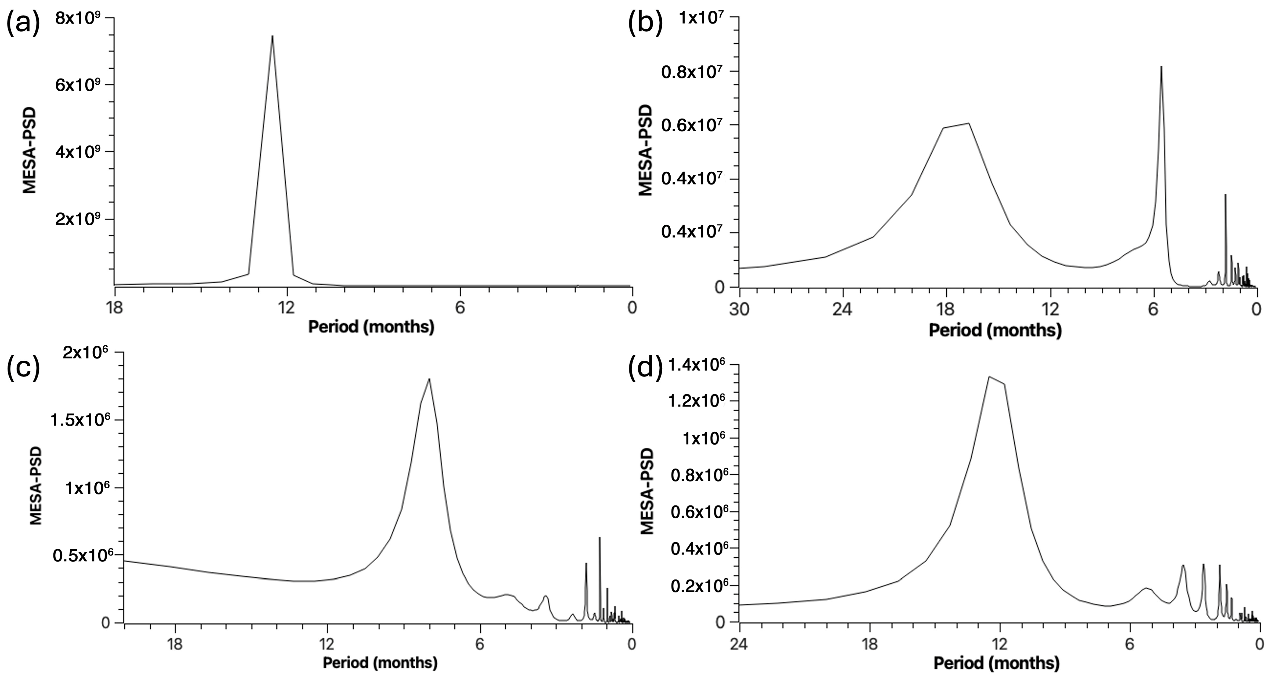
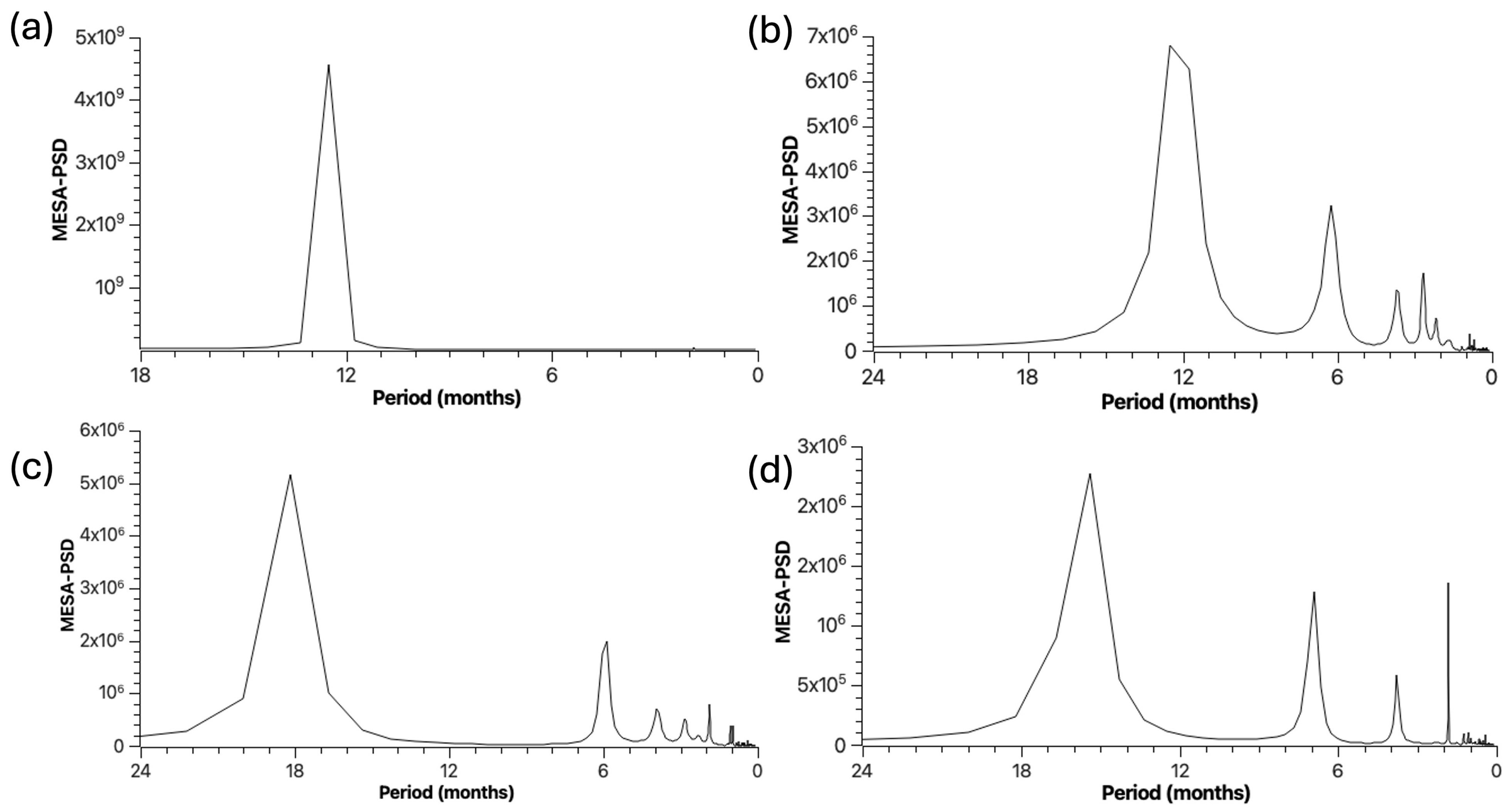
2.5. Maximum Entropy Spectral Analysis and Harmonic Prediction

Following the Box–Jenkins methodology, parametric time series models have been adopted as an advanced tool for the prediction of time series in the Autoregressive (AR) Integrated (I) Moving Averaged (MA) models [36,37]. The MA component is the noisy part, the I component addresses trends, and the autoregressive component (AR) represents what is considered the deterministic part of the model, suitable for stationary processes. Overseeing the parsimony principle, it is sufficient to use an AR model of a high enough order, p. Let a time series x(t) follow an autoregressive model of order p,

$$x\left(t\right)={\sum }_{n=1}^p{\mathrm{a}}_{n}x(t-n)$$

(6)

The coefficients a_n are the autoregressive coefficients, which are efficiently computed by the Burg’s algorithm verifying the Levinson recursion. The Maximum Entropy Spectral Analysis (MESA) involves the model of Equation (6) and its sine–cosine recursion. This results in a Fourier-like decomposition with sharply defined and very well-located peaks in terms of frequency ([18], Chapter 7 for the power spectral density properties and Chapter 8 for Burg’s algorithm). Due to the sharpness of the power spectral density produced by MESA (MESA-PSD), the frequencies use to be accurately estimated. A harmonic least-squares fitting on the time series of the temporal following the model:

$$A\left(t\right)=A_0+{\sum }_{i=1}^m(a_i·\cos \left({\omega }_{i}t\right)+b_i·\mathrm{s}\mathrm{i}\mathrm{n}({\omega }_{i}t\left)\right)$$

(7)

and this leads to the estimates of the cosine and sine amplitudes (a_i, b_i) with no possibility of confusion with the reflection coefficients of Equation (6). For this work, an eleven-terms moving window was used to select the frequencies to be considered in the harmonic fit.

Choosing the order of the AR model is a critical step in the analysis. Various criteria exist for estimating the appropriate order [18], including the Akaike Information Criterion (AIC) and the Minimum Description Length (MDL), both of which adhere to the principle of parsimony. However, according to Wold’s theorem, employing a non-parsimonious AR model can be beneficial, as a sufficiently high order will allow the spectrum to approximate a line spectrum with well-defined peak frequencies. It is inadvisable to use the “all poles method”, where the AR model order is set to half of the available data, due to the spontaneous line splitting. A practical guideline is to consider twice the expected number of components. In the absence of prior information, an initial estimate of one-quarter to one-third of the data length can be utilized. It is important to inspect the results carefully to prevent spontaneous line splitting. In this specific analysis, with a temporal mode length of 600, an AR order of 150 was selected. The MESA-PSD was then checked to ensure that spontaneous line splitting was avoided.

3. Results and Discussion

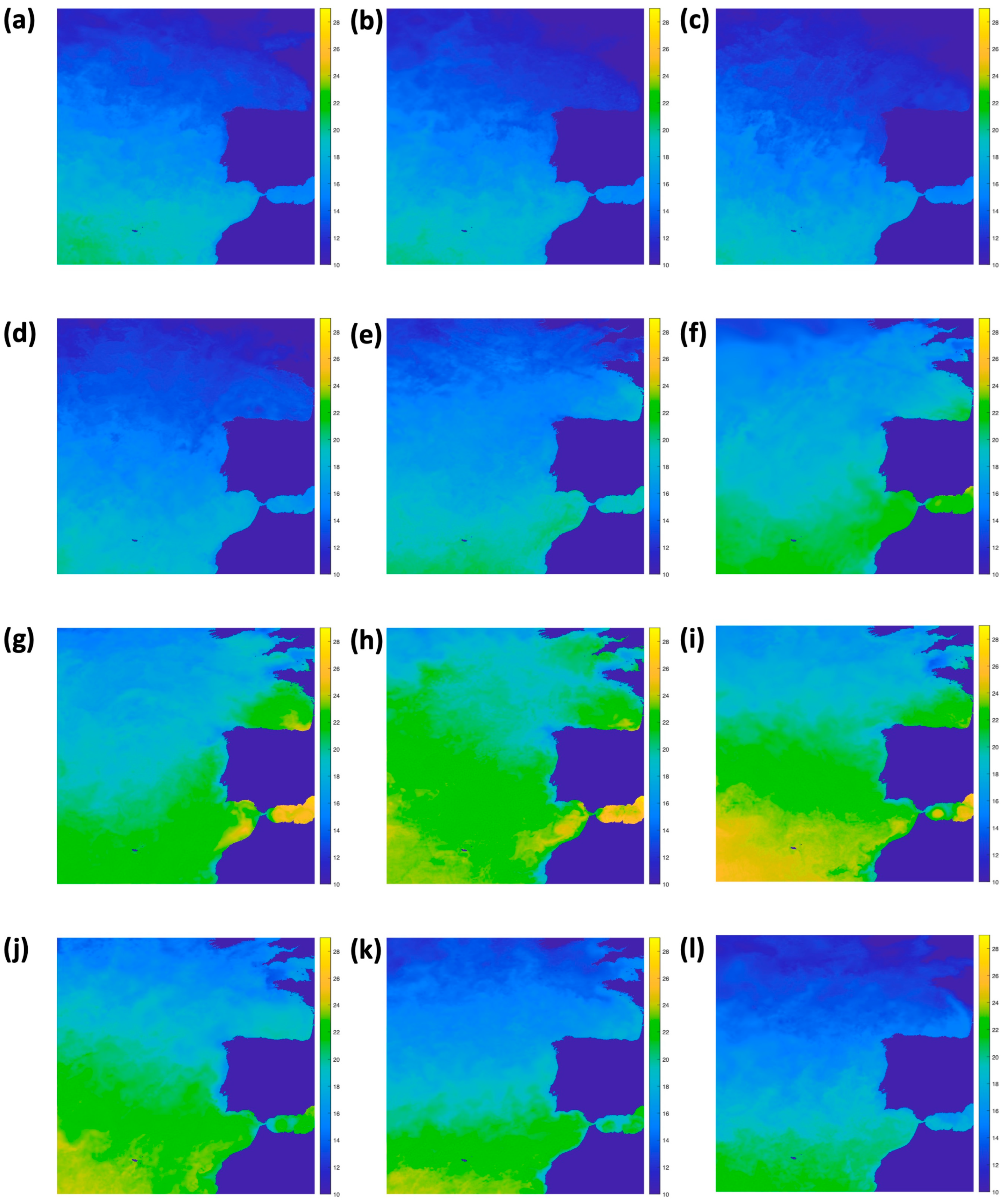
3.1. SST Imagery of the Whole ATLAZUL Area

A time series of the MUR-SST imagery for the entire ATLAZUL area is presented in Figure 2. The months from January to April (Figure 2a–d) exhibit similar patterns, showing cooler structures in the north. A preliminary inspection reveals no signature of cooler waters along the Galician coasts. In May and June (Figure 2e,f), indications of cooler waters begin to appear along the Galician and Portugal coasts. During the summer months, from July to October (Figure 2g–j), the Galician–Portuguese upwelling is observed according to [1,2,3,4,5,6]. In autumn, the cooler temperatures emerge again in November and December (Figure 2k,l), and the upwelling seems to diminish. This sequence shows the high variability in the SST signature, with seasonal changes in extent and values.

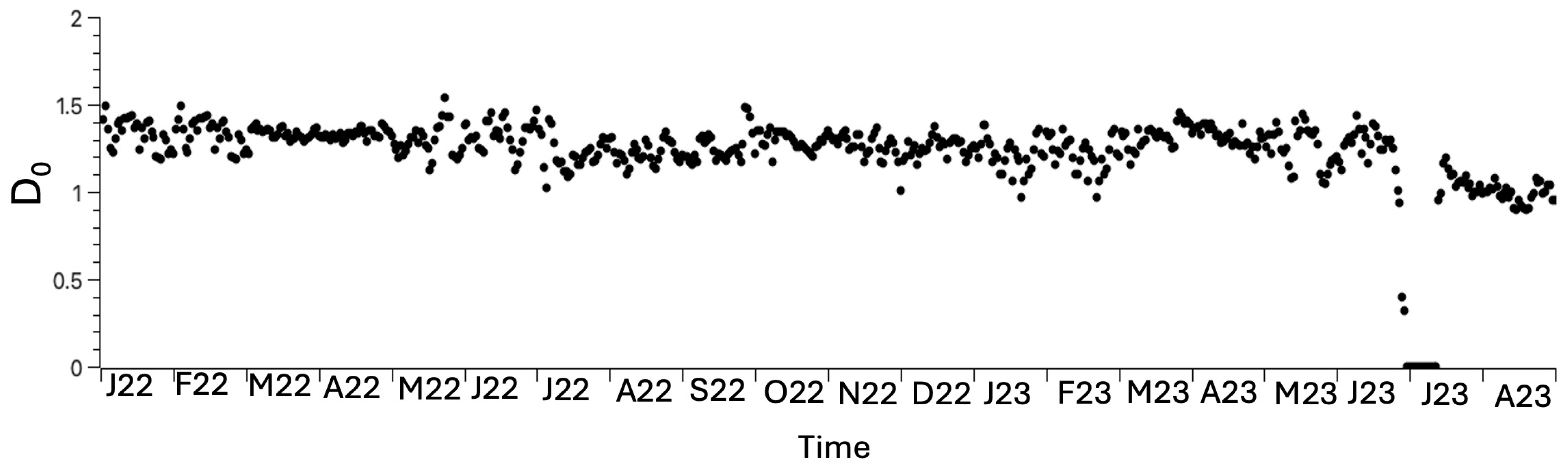
3.2. Area and Fractal Dimension

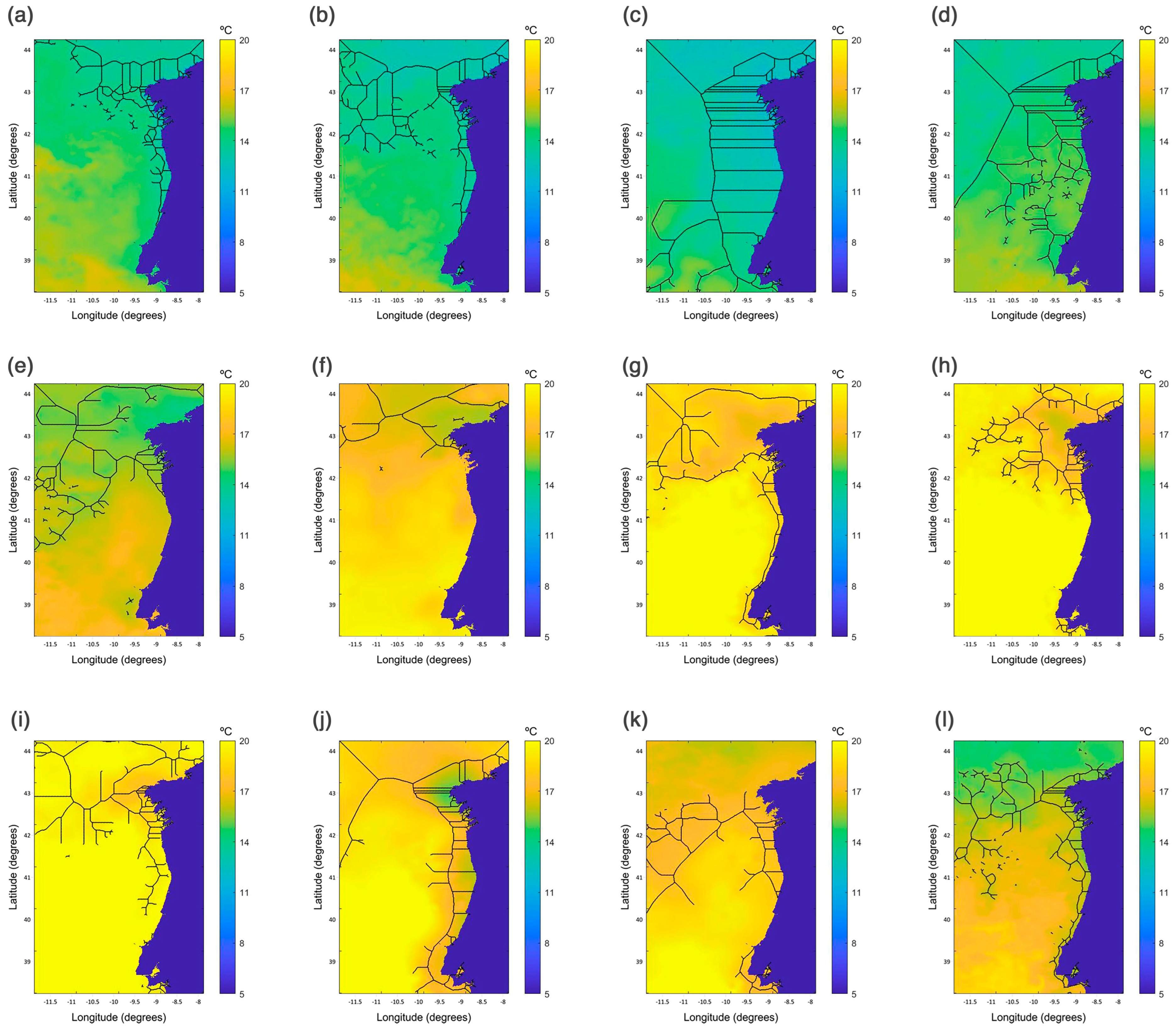
3.2.1. Galician–Portugal Region

The first analysis involves the computation of the area affected by upwelling along the Galician–Portugal coasts (see Figure 1). The north–south upwelling is characterized by surface temperatures ranging from 12 °C to 17 °C [1,6]. To more accurately isolate the SST signature, each image was visually inspected to establish a precise temperature interval for analysis. Following several trials and adjustments, a uniform interval of 12.5 °C to 14.9 °C was determined for all cases. The images were binarized with respect to the new interval of temperature, assigning one to pixels in the specified range and zero outside of it. Land was always excluded from the analysis. The total count of pixels serves as the indicator of the area. The time series of the area in the new range is depicted in Figure 3. The maximum area was observed in March of both 2022 and 2023, with addition peaks in October–November.

The morphological closing operator was applied on the binarized images to eliminate very small spatial structures and the quite common salt and pepper noise. This enhances the quality of the SST signature and facilitates the recovery of the skeleton by means of the Medial Axis Transform. The skeleton can be read as the path where the energy flows [12,13]. The question of how the space is filled, or how ordered/disordered the internal structure of the corresponding SST signature is, must be answered [10,11,12,13,38,39]. Figure 4 presents the skeletons of the SST signature along the Galician–Portugal coasts for the 15th of each month of 2022.

The skeleton position varies, sometimes further north or south, and its development fluctuates between more developed and contracted forms, yet it consistently branches along the coast. In other words, the SST signature between 12.5 °C and 14.9 °C exists throughout the year in the region, with a high variation in extension and intensity. A larger area correlates with a higher number of branches (Figure 4c,d for March and April, respectively, and Figure 3 for the same months in 2022).

The time series of the fractal dimension for the skeletons is presented in Figure 5. This has a consistent value of approximately 1.4. This suggests that the space is chaotically filled with many small-scale structures that can be observed or not.

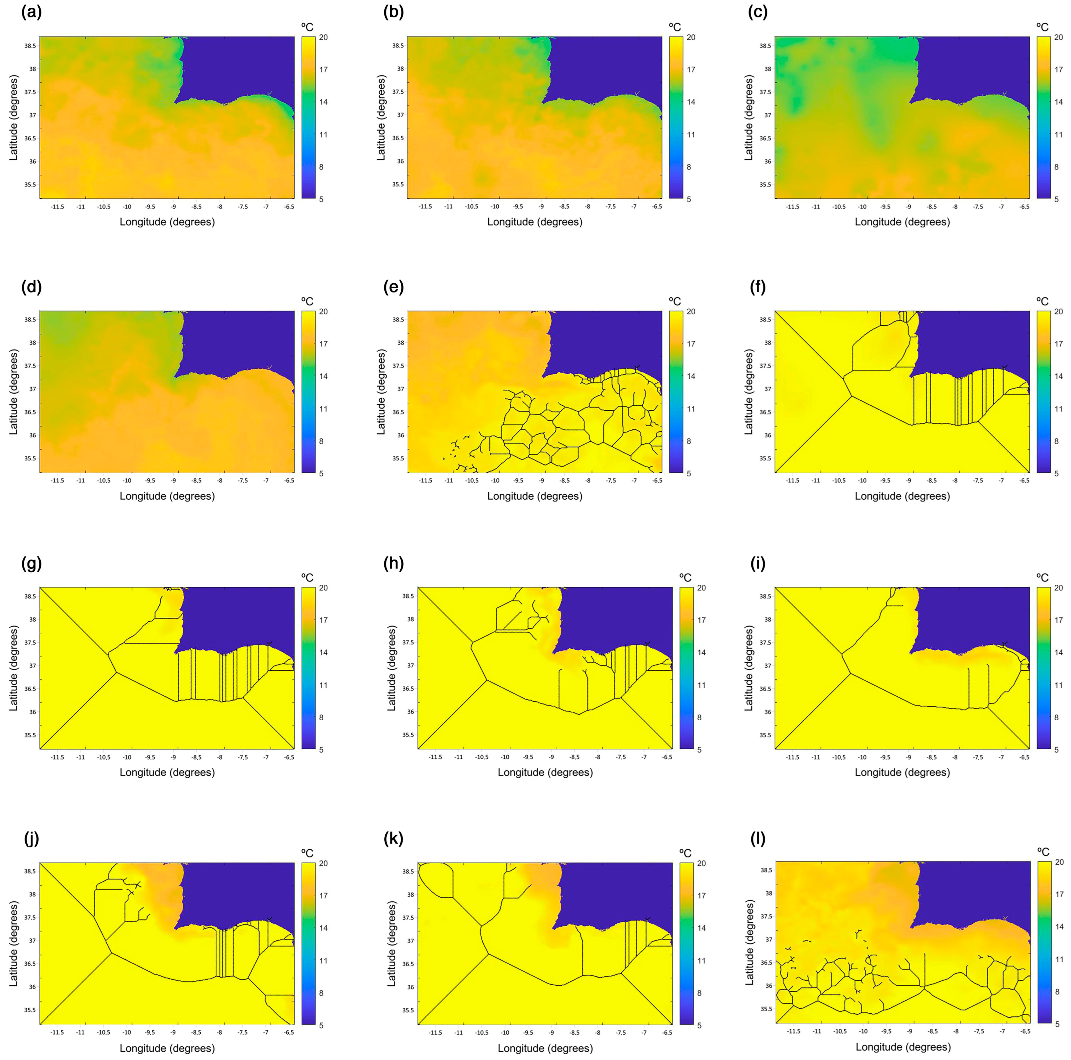
3.2.2. Gulf of Cádiz Region

There is no signature of the warmer water outflow in the Gulf of Cádiz during the months of January to April (Figure 2a–d). In May and June (Figure 2e,f), the Gulf of Cadiz begins to experience rising temperatures. Throughout the summer, from July to October (Figure 2g–j), the warmer waters dominate the entire area, with a distinct outflow signature from the shallow Bay of Cádiz. By autumn, in November and December (Figure 2k,l), the warmer water outflow disappears. As noted, the signature of the SST presents significant variability, with fluctuations in size and SST values across seasons.

The temperature of the warmer water outflow from the Bay of Cádiz to the Gulf typically ranges from 22 °C to 26 °C. Regarding the upwelling along the Galician–Portugal coasts, the area of the warm water outflow in the Gulf of Cádiz (see Figure 1) has been computed using the same methodology. Binarization was performed after a detailed visual inspection of each image, determining an interval for each one. After some trial and error, the resulting new interval was standardized between 20.0 °C and 25.3 °C. Land was also excluded from the analysis. The total pixel count is used as the indicator of the warm water area, and it is presented in Figure 6. There is no evidence of warm water from 22 January to 22 April. The area remains constant between 22 May and 22 December, and then the same values are newly present since 23 June. It is important to highlight the strong annual component in these patterns.

The morphological closing operator was again applied before using the Medial Axis Transform to recover the skeleton of the SST signature. The skeletons of the warmer water at the Gulf of Cadiz for the 15th of each month in 2022 are presented in Figure 7, complementing the analysis shown in Figure 6.

No warmer water signatures are observed from January to April 2022 (Figure 7a–d). Significant signatures appear between May and October (Figure 7e–j). There is a signature still present in 22 December (Figure 7l) attributable to the inflow–outflow dynamics from the Strait of Gibraltar. The fractal dimension remains relatively constant, with exceptions in the first four months (Figure 6) and in January, March and April 2023, during which the warmer water is not detected. The fractal dimension (Figure 8) has a value of 1.2, indicating that it has a little more organized flow while still with a high presence of chaotic structures.

3.2.3. Comparison between the Two Regions

Both ATLAZUL regions are very different in geometry and in influencing surrounding areas. The Galician–Portugal domain is oriented north–south with significant southward currents [1,2,3,4,5,6]. The area of the SST ranging from 12.5 °C to 14.9 °C shows a strong seasonal component (Figure 3) but with considerable variations. The fractal dimension of the skeletons of the SST signature point to a constant value of 1.4, meaning a chaotic way of space filling.

In contrast, the Gulf of Cádiz displays a clearer seasonal variation in the warm water outflow from the Bay of Cádiz (Figure 6). However, the influence of the Strait of Gibraltar can distort the SST signature in the open sea. An example is 22 December (Figure 7l) where the skeleton is due to the Atlantic and Mediterranean waters in the Gulf of Cádiz, with no significant branch observed near the coasts of the Bay of Cádiz. The fractal dimension has a value of 1.2 during the detection of this signature.

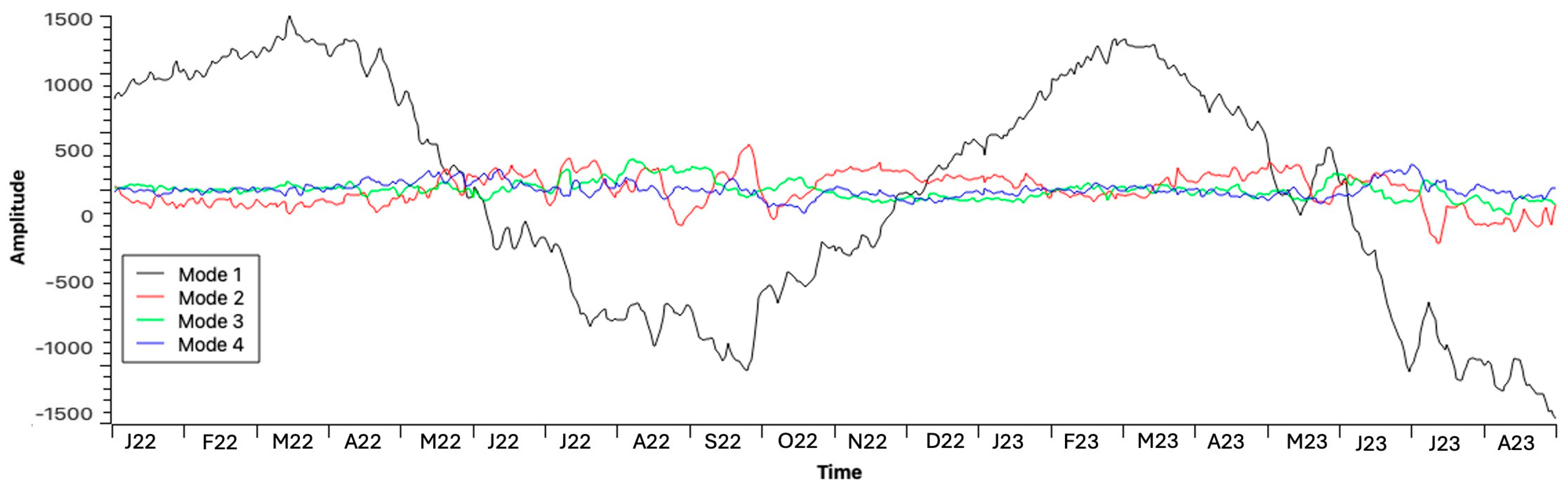
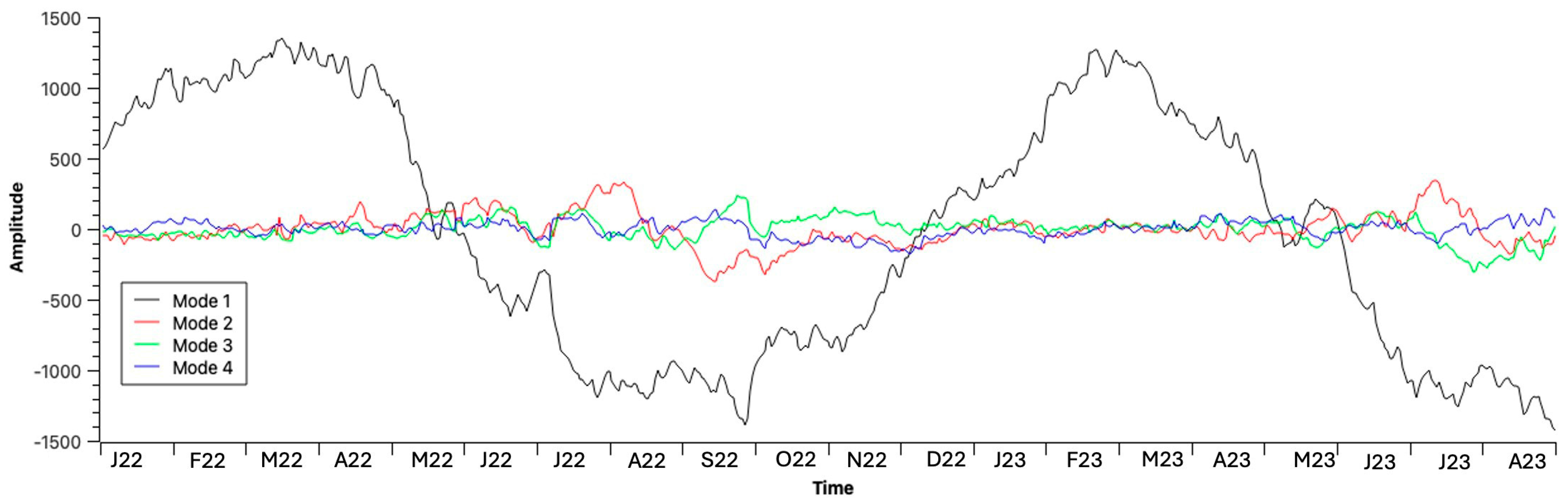
3.3. KLT/EOF Analysis

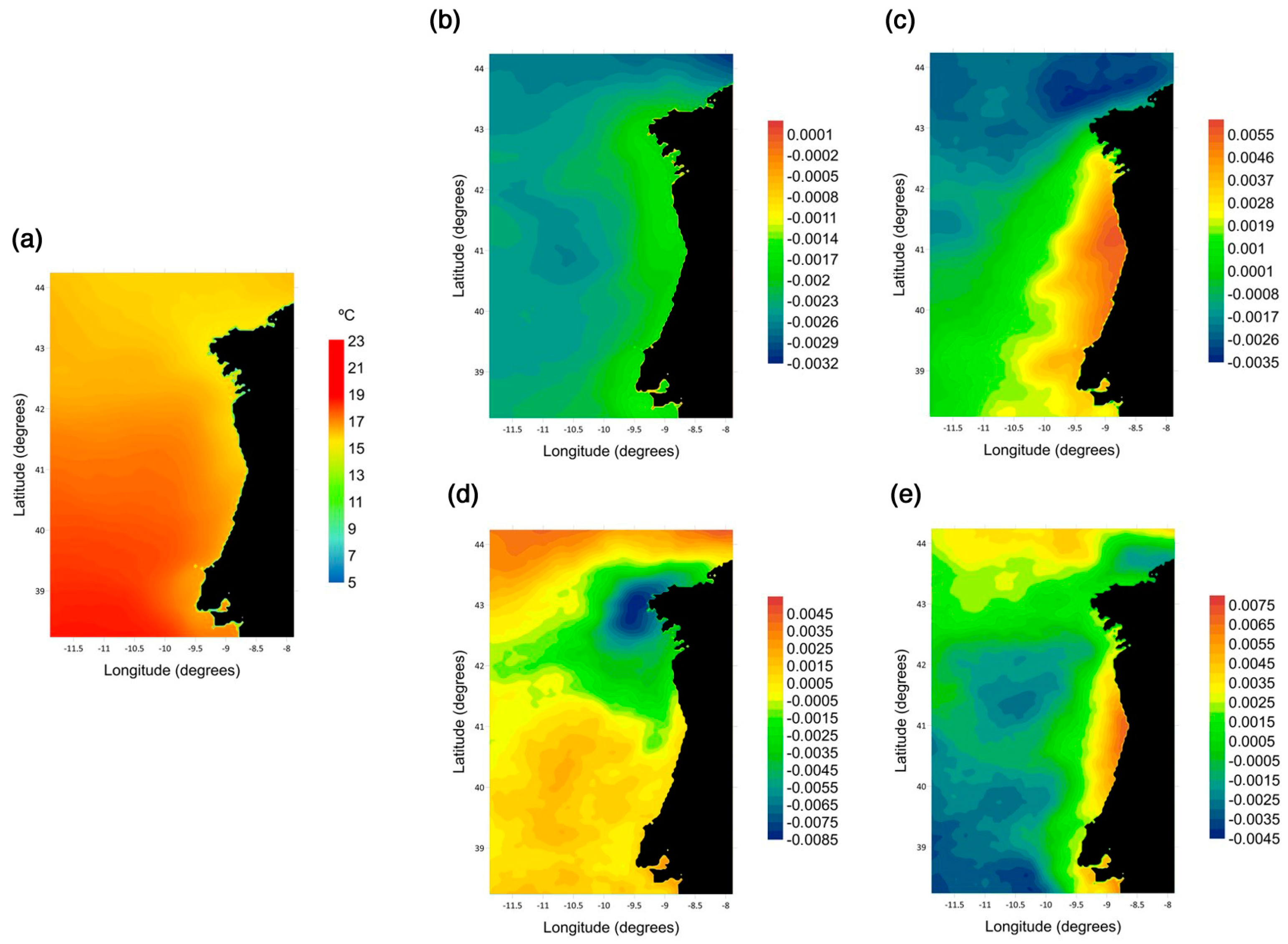
3.3.1. Galician–Portugal Region

By applying the KLT/EOF analysis on the MUR-SST anomaly imagery in the Galician–Portugal ATLAZUL region, the importance of the first four modes, computed from Equation (4), are presented in

Table 1. Importance, or percentage of explained variance, of the first four modes for the Galician–Portugal ATLAZUL region.

Order	Galician–Portugal (%)
1	95.03
2	2.19
3	0.6
4	0.42

.

The mean SST field and the first four spatial modes for the Galician–Portugal region are presented in Figure 9. The SST signature where the upwelling occurs is clearly observed in the mean field (Figure 9a). The first mode (Figure 9b) is quite homogeneous, and the second mode (Figure 9c) allows the establishment of the boundaries of the upwelling as in [6]. The third mode (Figure 9d) is more important around Finisterre Cape (see Figure 1) and the fourth mode (Figure 9e), almost negligible, points to the area where one of the cores of the upwelling happens [1,6].

The corresponding temporal modes are presented in Figure 10. The annual oscillation is clearly observed in the first mode. This represents 95% of the variance (Table 1). The rest of temporal modes have more shorter period components. Remarkable variations can be seen in September 2022, May 2023 and July 2023 in some of the four modes. These point out further work to be done.

The MESA-PSDs of the first four modes for the Galician–Portugal region (Figure 10) are shown in Figure 11. The first mode presents only one peak at the 12-month period with a very sharp peak (Figure 11a). The second one (Figure 11b) is composed by eighteen-, six- and three-month periods. The third one (Figure 11c) has a nine-month component and the rest are negligible. The fourth one (Figure 11d) presents an annual component and the rest of the peaks are very short-period contributions.

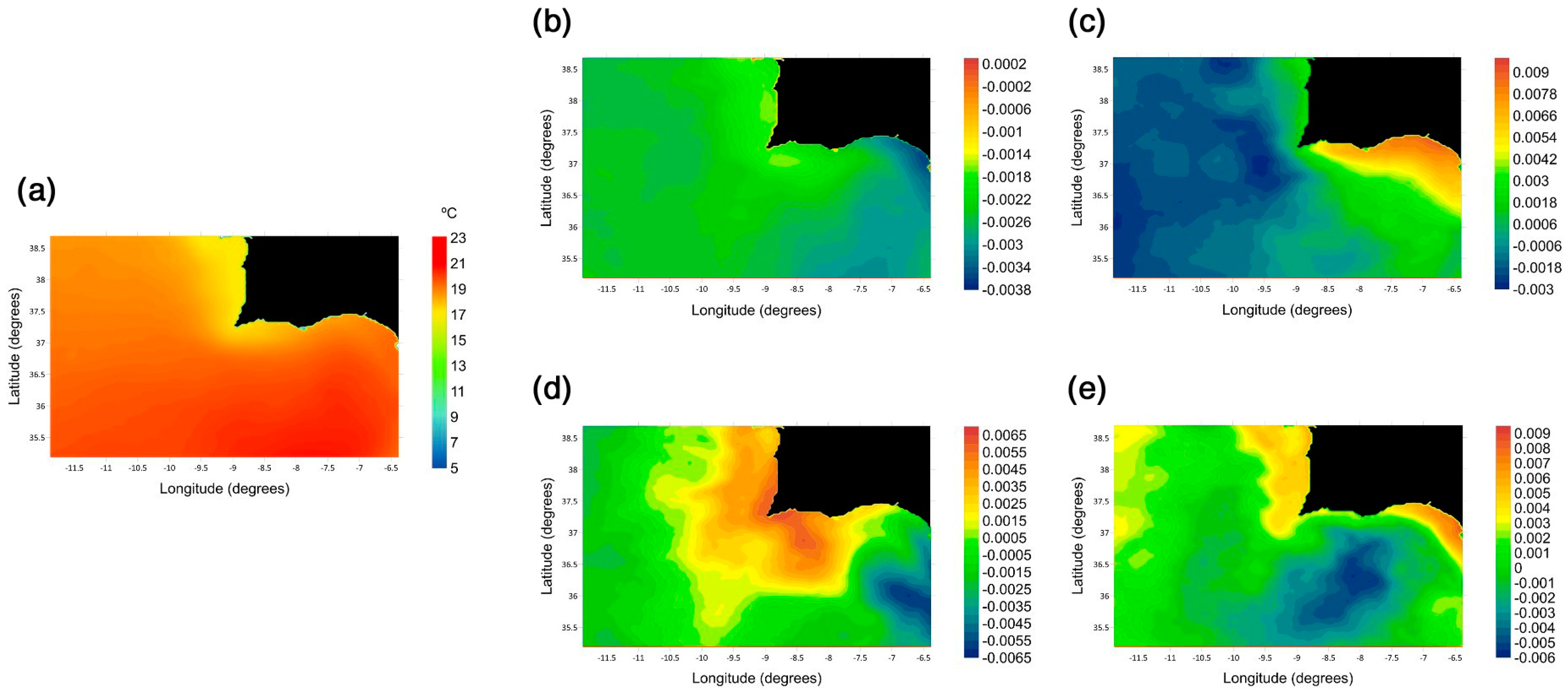
3.3.2. Gulf of Cádiz Region

By applying the KLT/EOF analysis on the MUR-SST anomaly imagery in the Gulf of Cádiz ATLAZUL region, the importance of the first four modes, computed from Equation (4), are presented in

Table 2. Importance, or percentage of explained variance, of the first four modes for the Gulf of Cádiz ATLAZUL region.

Order	Gulf of Cádiz (%)
1	94.81
2	1.77
3	0.88
4	0.41

. The first mode explains almost 95% of the variance and the sum of the other three explains about 3%.

The mean SST field and the first four spatial modes are presented in Figure 12. There is no trace of the warm water outflow from the Bay of Cádiz in the mean field (Figure 12a) nor in the first mode (Figure 12b). The second mode (Figure 12c) points to the separation of the coastal influence. The signature of the warmer outflow is observed in the third mode (Figure 12d), indicating that this is a second-order phenomenon. However, it is important for fisheries and for planning coastal activities, and it must be kept for prediction purposes.

The corresponding temporal modes are presented in Figure 13. The annual oscillation is also clearly observed in the first mode. The contributions from other modes are nosier and specific for each area. Remarkable variations can be seen in August 2022, September 2022 and May 2023 in some of the four modes. These point out further work to be done.

The MESA-PSD of the four first modes are shown in Figure 14 for the Gulf of Cádiz region (Figure 13). The first mode presents only one peak at the 12-month period with a very sharp peak (Figure 14a). The second (Figure 14b) is composed by twelve-, six-, four- and three-month periods. The third one (Figure 14c) has eighteen- and six-month components, and the rest are negligible. The fourth one (Figure 14d) presents sixteen-, seven-, five- and two-month components.

3.3.3. Comparison between the Two Regions

The importance of the modes is quite similar for both ATLAZUL regions (Table 1 and Table 2). The first mode explains about 95% of the variance and the sum of the other three explains about 3%.

The first important difference is in the first spatial mode. While the SST signature of coastal cooler waters in the Galician–Portugal region is present in the mean SST field (Figure 9a), there is no trace of the warm water signature in the mean SST field of the Gulf of Cádiz (Figure 12a). Now, the first modes (Figure 9b and Figure 12b) present the area affected by the upwelling [1] (Figure 9b) and by the warm water outflow (Figure 12b). However, the second modes allow the determination of the borders of the upwelling (Figure 9c) [1,6] and the coastal zone in the Gulf of Cádiz (Figure 12c). The third modes reveal secondary areas in the dynamic of each region, the Finisterre Cape (Figure 1 and Figure 9d) and San Vicente Cape (Figure 12d), but it is in the third mode where some signal of the warm water can be observed, meaning that this is a second-order phenomenon.

Regarding the temporal modes (Figure 10 and Figure 13), the first one is just the same for both ATLAZUL regions, even with the same amplitude. This clearly corresponds to the forcing of the entire ATLAZUL area. The other modes seem to be in antiphase.

It must be noticed that both years, 2022 and 2023, present different evolutions in what the second and third modes concern. The change happened in September 2022. This points out further work to be done.

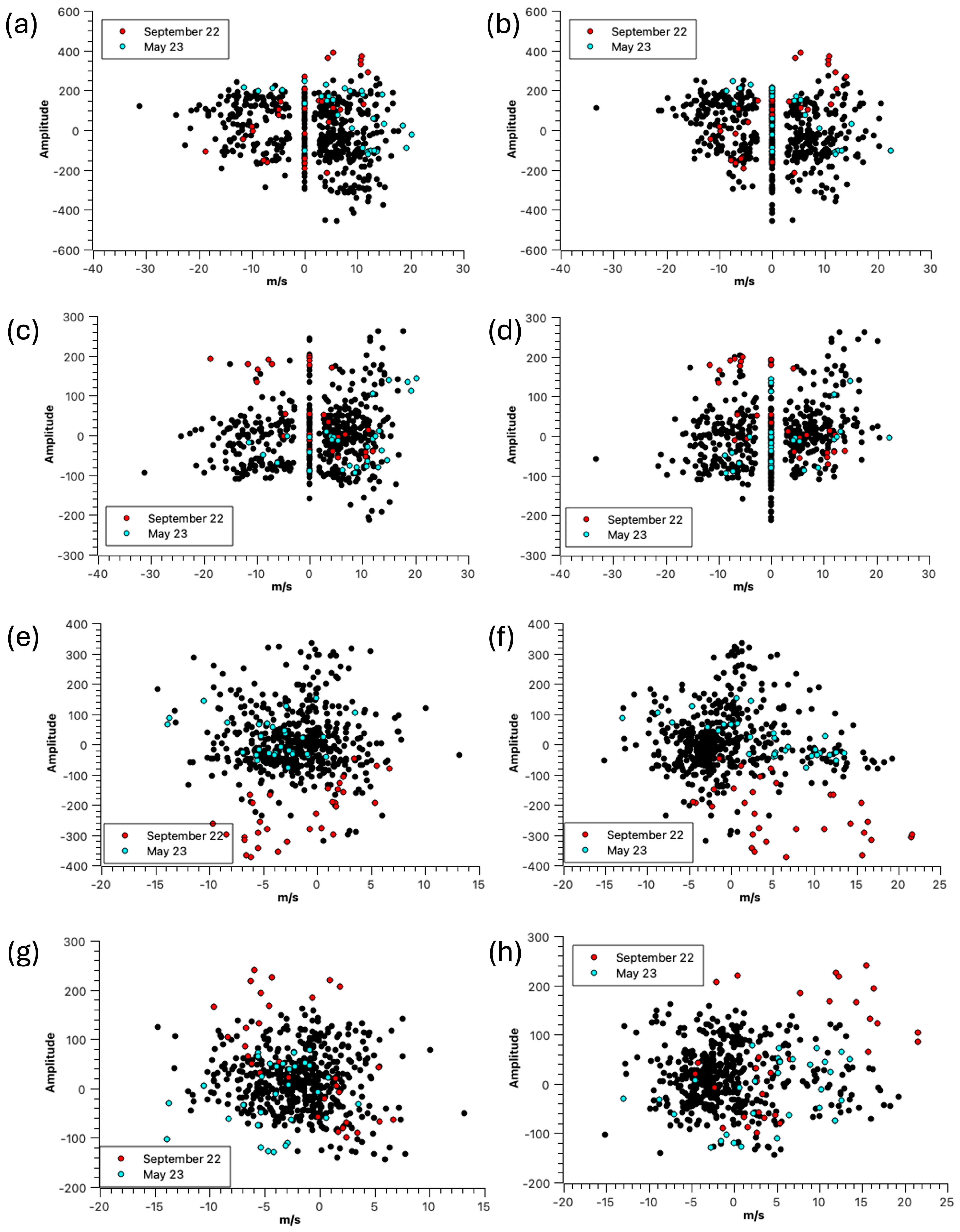
3.4. On the Effect of the Wind

The wind data were averaged to one data per day to be jointly analyzed with the data of the area affected by cooler waters, in the Galician–Portugal coasts, and by the warmer water signature in the Gulf of Cádiz. The vector plot of the wind at the Boya da Ribeira and at the Parque Natural Bahía de Cádiz are presented in Figure 15. The wind along the Portugal coasts blows in the north–south direction (Figure 15a) and in the Gulf of Cádiz is in the east–west direction (Figure 15b). The arrows have been rotated to facilitate the discussion. In any case, the role of the wind must be analyzed in three different ways. The first one is searching for a relationship between the time series of the affected area and the time series of the wind. Then, the comparison of the time series of the wind with the second and third modes of the KLT/EOF analysis is carried out.

3.4.1. Area

The wind in the Galician–Portugal ATLAZUL area mainly blows in the north–south direction. It must be wait that when blowing southward the upwelling be active. From the results of Section 3.2, it seems as if the area affected with an SST signature between 12.5 °C and 14.9 °C is not related to the wind. For example, the maximum area is in March–April 2022 (Figure 3), but in those months the wind is northward (Figure 15a). However, the wind blows southward in October–November 2022 (Figure 15a) when a maximum area occurs (Figure 3), as in March 2023.

We focus the attention on September 2022 and May 2023, when the second and third modes seem to be more variable. The scatter plot between the cross-shore wind and the area of the cooler waters in the Galician–Portugal region is presented in Figure 16a. The denser point concentration is when the velocity is positive, and the area is smaller than half of the maximum. A double point cloud with positive and negative velocities is observed in the case of the along-shore wind (Figure 16b). The data for September 2022 (red dots) and May 2023 (blue dots) are located in the small or half maximum area and cover all of the wind intensities (Figure 16a,b).

The correlation between the components of the wind and the area for the September 2022 and May 2023 are detailed in

Table 3. Correlation between the along-shore and cross-shore components of the wind with the area for the months of September 2022 and May 2023 for the Galician–Portugal region.

Wind Component	Month	Correlation
Along-shore	September 2022	0.9564
Along-shore	May 2023	0.8736
Cross-shore	September 2022	0.9566
Cross-shore	May 2023	0.8716

to quantify their relationships in the Galician–Portugal region. It seems that there is no connection between wind and area (Figure 16a,b) and the zero velocity corresponds to possible instrumental errors when the analysis is focused in a short period. The correlation in September 2022 exceeds 0.95 and it is better than for May 2023 with a value of 0.87. This ensures the relationship between wind and area.

This is clearer for the Gulf of Cádiz. The scatter plot between the along-shore wind and the area of the warmer waters (Figure 16c) shows a dense point cloud with high area values and positive velocities (blowing eastward). It seems to have no relation between the cross-shore wind and the area of the warmer waters (Figure 16d) with a denser point cloud around zero velocity. In addition, while the data for September 2022 (red dots) spread over a variety of wind conditions and the area of the warmer waters, the data of May 2023 are well located in the maximum size. This ensures the relationship between wind and area in that month (Figure 16c,d).

The correlation between the components of the wind and the area for September 2022 and May 2023 are detailed in

Table 4. Correlation between the along-shore and cross-shore components of the wind with the area for the months of September 2022 and May 2023 for the Gulf of Cádiz region.

Wind Component	Month	Correlation
Along-shore	September 2022	0.9989
Along-shore	May 2023	0.999
Cross-shore	September 2022	0.9188
Cross-shore	May 2023	0.9079

for the Gulf of Cádiz to quantify their relationships. The correlation in September 2022 and May 2023 exceeds 0.99 for the along-shore component, but for May 2023 it is around 0.9.

It must be noticed that the wind components are not rotated and both components must present some relationship with the area and these results can be biased due to the presence of the first mode.

3.4.2. The Second and Third Modes

The results of the KLT/OF analysis were presented in Section 3.2. The first temporal mode was identified with the annual period. The second and third modes may be related to smaller spatiotemporal scale phenomena and the fourth mode can be considered negligible.

Concerning the Galician–Portugal ATLAZUL region, and from a visual inspection of the time series of the wind (Figure 15a) with the second and third temporal modes (Figure 10) and the same spatial modes (Figure 9), the temporal modes are quite constant from January–April 2022. When the amplitude of the second temporal mode increases (22 July–September) is when the wind blows northward. Other maxima are in October–November 2022 and the wind blows southward. The corresponding spatial mode has positive weights in those months, increasing the signal. It is remarkable that the third spatiotemporal mode (Figure 9 and Figure 10) has the antiphase behavior with the second mode. Hence, the wind effect is reflected in the second and third modes.

This happens in the same way with the Gulf of Cádiz ATLAZUL region. The difference is that the spatiotemporal modes (Figure 12c,d and Figure 13) present different signs.

The relationships of the cross and along-shore winds with the second and third temporal modes are investigated in Figure 17.

For the Galician–Portugal region, the scatter plot between the cross-shore wind and the second mode is presented in Figure 17a and the along-shore wind with the second mode is presented in Figure 17b. There is not a clear relationship between the amplitude of the second mode and the north–south wind. Focusing the attention on the data for September 2022, these spread all over the range of amplitude and wind but the data corresponding to May 2023 are in the maximum values of the amplitude of the second mode, relating periods of higher amplitude with the north–south wind component (Figure 17a).

The relation of the cross-shore wind with the third mode is presented in Figure 17c and the same, but considering the along-shore current, is shown in Figure 17d. Both point out some weak relationship where the data for September 2022 seems to be related to the higher amplitudes and those for 23 May to the lower amplitudes. However, this is not clear enough due to the variability of the action of the wind in this ATLAZUL region.

On the other hand, there is a relationship between the cross-shore and along-shore wind with the data of 22 September and the second mode for the Gulf of Cádiz region (Figure 17e,f respectively), being especially clear with the along-shore component (Figure 17f). This month corresponds to when the warmer water outflow is established in the Gulf of Cádiz. In the case of 23 May, the cloud point is more spread and corresponds to minimum amplitudes in the second mode. All of this leads to considering some relationship between the wind and the second mode.

The cross-shore wind seems not to be related to the third mode (Figure 17g). However, the along-shore wind is clearly related to the third mode (Figure 17h) with high positive amplitudes and high winds. This can be observed in the distribution of the data of 22 September and 23 May. The first ones had the highest amplitudes, and the last ones had the negative ones. The combined action of the second and third modes in the along-shore wind component seems to be responsible for the warmer water outflow from the Bay of Cádiz.

The linear correlations between the wind components and the amplitudes of the second and third modes for both regions and for the months of September 2022 and May 2023 are presented in

Table 5. Correlation between the along-shore and cross-shore components of the wind and the amplitudes of the second and third modes for the months of September 2022 and May 2023. The first correlation is for September 2022 and the second is for May 2023.

	Wind Component	Mode 2	Mode 3
Galician–Portugal	Along-shore Cross-shore	0.4446/0.4966 0.5639/0.5836	0.5945/0.2137 0.6346/0.1573
Gulf of Cádiz	Along-shore Cross-shore	0.9314/0.1108 0.8908/0.5724	0.5273/0.1012 0.4371/0.2026

. It seems that the area of the cooler waters along the Galician–Portugal coasts is more related to the third mode and to September 2022, being negligible in May 2023. However, the second mode presents some influence.

The warmer water outflow for the Gulf of Cádiz is related to the second mode in both analyzed months, but the third mode must be also considered.

The authors have not seen any relationship (none presented) between the wind components and the fourth mode for either ATLAZUL region.

In summary, while the episodic nature of the wind is complex, there may be potential to utilize the KLT/EOF to search for a further exploration of relationships, mainly focusing on the second and third modes within the ATLAZUL area.

3.5. Prediction

3.5.1. Harmonic Model Prediction

The natural way to take advantage of the results of the KLT/EOF is exploding the harmonic nature of the temporal modes. With this, a harmonic prediction model can be carried out by predicting the temporal modes and reconstructing the SST field at any time.

The harmonic prediction involves the following steps: (i) compute the MESA-PSD for the temporal weights A(t) (Section 2.4); (ii) isolate the peak frequencies identified in the power spectral densities; (iii) perform the harmonic decomposition (sine and cosine amplitudes, Equation (7)) by least squares fitting; (iv) use the derived sine and cosine amplitudes to predict the different temporal modes; (v) reconstruct the SST anomaly fields, adding the SST mean field to obtain the complete the SST prediction; and (vi) compute the correlation between observed and predicted SST fields.

3.5.2. Results and Discussion

Utilizing the peak frequencies identified in Figure 11 and Figure 14, a least square fitting on Equation (6) computes the sine and cosine amplitudes. These are used to predict the temporal weights. Incorporating the mean SST fields to the predicted SST anomaly fields, the prediction of the SST is generated. We have considered the first 600 snapshots as the training field to predict the subsequent 38 fields. The correlations between observed and predicted SST fields are presented in Figure 18 (red line). They are calculated without bias from land influence.

The lowest observed correlation is for the Galician–Portugal region at the beginning of the prediction period (Figure 18). The values rise to approximately 0.9, improving the accuracy for long-term prediction. In contrast, the Gulf of Cádiz presents consistent high correlation values with maxima higher exceeding 0.9 and an average around 0.8. It must be noticed that the long-term prediction is possible due to several reasons. The first mode represents a very high percentage of the variance (Table 1 and Table 2) and it is clearly harmonic (Figure 10, Figure 11, Figure 12, Figure 13 and Figure 14) with a very sharp peak in the power spectral density. The second and the third modes represent about 2.7% but the energy spectra are very well defined. The matrix condition for the different least squares fit on Equation (6) has values of about 2.3 for the first to the third temporal weight and about three for the fourth one, pointing, in general, to the good separability among harmonic components.

The observed SST fields and the spatial distribution of the errors in the prediction for 10, 20, 30 and 38 days ahead for both regions are presented in Figure 19. For the short term, the quality of the prediction is lower for the Galician–Portugal ATLAZUL region; however, the long-term predictions for both regions are quite reliable.

In the Gulf of Cádiz, the errors at time ten of prediction (Figure 19b) underestimate the observed SST (Figure 19a), particularly near the coast, with a correlation about 0.8 (Figure 18). By day 20, the correlation is about 0.85 with a substantial area with near-zero prediction errors (Figure 19c,d). Regions near the coast are underestimated and regions far from San Vicente Cape are overestimated. The same structure is observed for 30 day (Figure 19e,f) and 38 day (Figure 19g,h).

Regarding the Galician–Portugal coasts, the correlation starts with low values (Figure 18), reaching 0.75 by the tenth day, indicating high prediction errors (Figure 19i,j). Something similar is observed at day 20 (Figure 19k,l) and it is slightly improved at day 30 (Figure 19m,n). By day 38, the correlation reaches a value exceeding 0.9 (Figure 18) and the magnitude of the errors decreases compared with earlier forecasts (Figure 19o,p).

The errors between observed and predicted SST fields can be due to the weight of the time series of the second and the third modes. Both have large variability as shown in Figure 9c,d, and are largely affected by wind, for which the effects are not periodic and cannot be easily included in the harmonic prediction model. The inclusion of external bearings in the prediction model is an open task for future work.

4. Conclusions

From the analysis of a time series of digital imagery of SST for the ATLAZUL area, it is possible to conclude that: (i) the tow upwelling areas are identified along the Galician–Portugal coast as the second and third modes of KLT/EOF analysis, and they are partially affected by wind, exhibiting large variations throughout the year; (ii) the tow warm water outflows from the Bay of Cádiz to the Gulf of Cádiz are identified as the second and third modes of KLT/EOF analysis, partially affected by wind as well; (iii) the skeletons of the surface signature of the upwelling and of the warmer water outflow and their fractal dimensions point to a chaotic way to fill the space; and (iv) the harmonic prediction model should be combined with the wind prediction.

The present study provides useful knowledge and products to the public and private actors along the Galician–Portugal and Gulf of Cádiz ATLAZUL regions, and it may be of interest to ocean and coastal waters research groups, for environmental researchers and for fisheries and environmental management in the whole ATLAZUL area.

References

1. Haynes, R.; Barton, E.D.; Pilling, I. Development, persistence and variability of upwelling filaments off the Atlantic coast of the Iberian Peninsula. J. Geophys. Ocean. Res. 1993, 98, 22681–222692. [Google Scholar] [CrossRef]
2. Pérez, F.F.; Castro, C.G.; Álvarez-Salgado, X.A.; Ríos, A.F. Coupling between the Iberian basin-scale circulation and the Portugal boundary current system: A chemical study. Deep. Sea Res. Part I Oceanogr. Res. Pap. 2001, 48, 1519–1533. [Google Scholar] [CrossRef]
3. Martins, C.S.; Hamann, M.; Fiúza, F.F.G. Surface circulation in the eastern North Atlantic from drifters and altimetry. J. Geophys. Ocean. Res. 2002, 107, 3217. [Google Scholar] [CrossRef]
4. Peliz, A.; Dubert, J.; Santos, A.M.P.; Oliveira, P.B.; Le Cann, B. Winter upper ocean circulation in the western Iberia basin- fronts, eddies and poleward flows: An overview. Deep Sea Res. I 2005, 52, 621–646. [Google Scholar] [CrossRef]
5. Arístegui, J.; Álvarez-Salgado, X.A.; Barton, E.D.; Figueiras, F.G.; Hernández-León, S.; Roy, C.; Santos, A.M.P. Oceanography and fisheries od the Canary current/Iberian region of the eastern North Atlantic. In The Sea; Robinson, A., Brink, K.H., Eds.; Harvard University Press: Cambridge, MA, USA, 2004; Volume 14. [Google Scholar]
6. Relvas, P.; Barton, E.D.; Dubert, J.; Oliveira, P.B.; Pleiz, A.; da Silva, J.C.B.; Santos, A.M.P. Physical oceanography of the western Iberia ecosystem: Latest views and challenges. Prog. Oceanogr. 2007, 74, 149–173. [Google Scholar] [CrossRef]
7. Criado-Aldanueva, F.; García-Lafuente, J.; Navarro, G.; Ruiz, J. Seasonal and interanual variability of the Surface circulation in the eastern Gulf of Cádiz (SW Iberia). J. Geophys. Ocean. Res. 2009, 114, C01011. [Google Scholar] [CrossRef]
8. Nolasco, R.; Cordeiro, P.; Cordeiro, N.; Le Cann, B.; Dubert, J. A high-resolution modeling study of the western Iberian margin mean and seasonal upper ocean circulation. Ocean. Dyn. 2013, 63, 1041–1062. [Google Scholar] [CrossRef]
9. Serrano, M.A.; Cobos, M.; Magaña, P.J.; Díez-Minguito, M. Sensitivity of Iberian estuaries to changes in sea water temperature, salinity, river flow, mean sea level and tidal amplitude. Estuar. Coast. Shelf Sci. 2020, 236, 106624. [Google Scholar] [CrossRef]
10. Alonso, J.; Blázquez, E.; Isaza, E.; Vidal, J. Internal structure of the upwelling events at Punta Gallinas (Colombian Caribbean) from MODIS-SST imagery. Cont. Shelf Res. 2015, 109, 127–134. [Google Scholar] [CrossRef]
11. Alonso, J.; Vidal, J.; Blázquez, E. On the prediction of upwelling events at the Colombian Caribbean coasts from MODIS-SST imagery. Sensors 2019, 19, 2861. [Google Scholar] [CrossRef]
12. Blázquez, E.; Alonso, J.; Vidal, J. On the Correlation of Sea Surface Temperature and Chlorophyll in Upwelling Events from Satellite Imagery. Oceanogr. Fish. 2017, 5, 15–18. [Google Scholar] [CrossRef]
13. Blázquez, E.; Alonso, J.; Vidal, J. On the sensitivity of the fractal dimension of the skeleton of sea surface temperature signatures from upwelling events on spatial resolution and threshold: Application on imagery of the Caribbean Sea. Int. J. Remote Sens. 2017, 38, 371–390. [Google Scholar] [CrossRef]
14. Hotelling, H. Analysis of a complex of statistical variables into principal components. J. Educ. Psychol. 1953, 24, 417–441. [Google Scholar] [CrossRef]
15. Thomson, R.E.; Emery, W. Data Analysis Methods in Physical Oceanography, 3rd ed.; Elsevier: New York, NY, USA, 2014. [Google Scholar]
16. Fukunaga, K. Introduction to Statistical Recognition; Academic Press: Cambridge, MA, USA, 1990. [Google Scholar]
17. Orfanidis, S.J. Introduction to Signal Processing; Prentice Hall: Upper Saddle River, NJ, USA, 1996. [Google Scholar]
18. Marple, S.L. Digital Spectral Analysis with Applications; Prentice Hall: Sydney, Australia, 1987. [Google Scholar]
19. Serra, J. Image Analysis and Mathematical Morphology; Academic Press: London, UK, 1982; Volume I. [Google Scholar]
20. Serra, J. Mathematical Morphology and Image Analysis; Academic Press: London, UK, 1988; Volume II. [Google Scholar]
21. Soille, P. Morphological Image Analysis: Principles and Applications, 2nd ed.; Springer: Berlin/Heidelberg, Germany, 2003. [Google Scholar]
22. Soille, P. Morphological Image Analysis; Springer: Berlin/Heidelberg, Germany, 2004. [Google Scholar]
23. Toshio, M.C.; Vazquez, J.; Armstrong, E.M. A multi-scale high-resolution analysis of global sea surface temperature. Remote Sens. Environ. 2017, 200, 154–169. [Google Scholar] [CrossRef]
24. Karhunen, K. Zur Spektraltheorie Stochastischer Prozesse; Annales Academia Science Fennicae: Helsinki, Finland, 1946; p. 37. [Google Scholar]
25. Loève, M.M. Probability Theory; Van Nostrand: Princeton, NJ, USA, 1955. [Google Scholar]
26. Burl, J.B. Reduced-order system identification using the Karhunen-Loève transform. Int. J. Model. Simul. 1993, 13, 183–188. [Google Scholar] [CrossRef]
27. Yamashita, Y.; Ogawa, H. Relative Karhunen-Loève Transform. IEEE Trans. Signal Process. 1996, 44, 371. [Google Scholar] [CrossRef]
28. Kirby, M.; Sirovich, S. Application of the Karhunen-Loève Procedure for the characterization of human faces. IEEE Trans. Pattern Anal. Mach. Intell. 1990, 12, 103–108. [Google Scholar] [CrossRef]
29. Murase, H.; Nayar, S. Visual learning and recognition of 3-D objects from appearance. Int. J. Comput. Vis. 1995, 14, 5–24. [Google Scholar] [CrossRef]
30. Berberian, S.K. Introduction to Hilbert Spaces; Oxford University Press: Oxford, UK, 1961. [Google Scholar]
31. Abellanas, L.; Galindo, A. Espacios de Hilbert; Eudema, S.A., Ed.; Universidad Complutense de Madrid: Madrid, Spain, 1987. [Google Scholar]
32. Maragos, P.; Schafer, R. Morphological filters–part I: Their Set-theoretic Analysis and Relations to Linear Shift-invariant Filters. IEEE Trans. Acoust. Speech Signal Process. 1987, 35, 1153–1169. [Google Scholar] [CrossRef]
33. Mendiola-Santibáñez, J.D.; Terol-Villalobos, I.R. Morphological Contrast Enhancement Using Connected Transformations. Proc. SPIE 2002, 4667, 365–376. [Google Scholar]
34. Falconer, K. The Geometry of Fractal Sets; Cambridge University Press: Cambridge, UK, 1985. [Google Scholar]
35. Falconer, K. Fractal Geometry: Mathematical Foundations and Applications, 2nd ed.; Wiley: Chichester, UK, 2003. [Google Scholar]
36. Peña Sánchez de Rivera, D. Análisis de Series Temporales; Alianza Editorial: Madrid, Spain, 2005; ISBN 978-84-206-9128-2. [Google Scholar]
37. Vandaele, W. Applied Time Series and Box-Jenkins Models; Academic Press: Orlando, FL, USA, 1983; ISBN 0127126503. [Google Scholar]
38. Alonso, J.J. On the Fractal Dimension of Earth Tides and Characterization of Gravity Stations. Bull. D’informations Marees Terr. 1998, 129, 9963–9973. [Google Scholar]
39. Alonso, J.J.; Vidal, J.M.; Blázquez, E. Why Are the High Frequency Structures of the Sea Surface Temperature in the Brazil–Malvinas Confluence Area Difficult to Predict? An Explanation Based on Multiscale Imagery and Fractal Geometry. J. Mar. Sci. Eng. 2023, 11, 1096. [Google Scholar] [CrossRef]
Figure 1. Atlantic Iberian coasts. The ATLAZUL area comprises the Spanish coasts (Galicia and the Gulf of Cádiz) and the coast of Portugal (North, Centre, Lisbon, Alentejo and Algarve). The three more important reference points are the Finisterre and San Vicente Capes and the Strait of Gibraltar. The western limit has been considered at the longitude of Madeira Island. The false color MUR images correspond to 1 August 2022. A signature of cooler water along the Galician and Portuguese coasts is observed along the Galician–Portugal coasts (clear blue) and the warmest water outflow (yellow) in the Gulf of Cádiz. The black solid arrow indicates the location of Boia da Ribeira and the white point indicates the meteorological station located at the Parque Natural Bahía de Cádiz.
Jmse 12 01580 g001
Figure 2. A sequence of the SST fields in the ATLAZUL area for the first day each month in 2022. (a) January to (l) December. Temperature in Celsius degrees. A signature of cooler water is easily seen along the Galician and Portugal coasts (g) to November, (k) with cooler water (in blue) and the warm water output in the Gulf of Cádiz from July (g) to September (in yellow).
Jmse 12 01580 g002
Figure 3. Time series of the area of the upwelling along the Galician–Portugal coasts.
Jmse 12 01580 g003
Figure 4. MUR-SST fields and the skeletons for the Galician–Portugal coasts corresponding to day 15 of each month of 2022 from (a) January to (l) December. Temperature is in Celsius degrees.
Jmse 12 01580 g004
Figure 5. Time series of the fractal dimension of the skeletons along the Galician–Portugal coasts.
Jmse 12 01580 g005
Figure 6. Time series of the area of the warm water output in the Gulf of Cádiz.
Jmse 12 01580 g006
Figure 7. MUR–SST fields and the skeletons for the Gulf of Cádiz corresponding to day 15 of each month of 2022 from (a) January to (l) December. Temperature is in Celsius degrees.
Jmse 12 01580 g007
Figure 8. Time series of the fractal dimension of the warm water output in the Gulf of Cádiz.
Jmse 12 01580 g008
Figure 9. (a) Mean SST field and the first four spatial modes (be), for the ATLAZUL region of Galician–Portugal coasts.
Jmse 12 01580 g009
Figure 10. Temporal weights for the Galician–Portugal ATLAZUL region.
Jmse 12 01580 g010
Figure 11. MESA-PSD of the temporal weights for the first (a) to the fourth (d) mode for the Galician–Portugal region.
Jmse 12 01580 g011
Figure 12. (a) Mean SST field and the first four spatial modes (be), for the ATLAZUL region of the Gulf of Cádiz.
Jmse 12 01580 g012
Figure 13. Temporal weights for the Gulf of Cádiz ATLAZUL region.
Jmse 12 01580 g013
Figure 14. MESA-PSD of the temporal weights for the first (a) to the fourth (d) mode for the Gulf of Cádiz region.
Jmse 12 01580 g014
Figure 15. Vector plot of the daily averaged wind time series taken at (a) Boia da Ribeira, La Coruña, and (b) Observatorio del Parque Natural Bahía de Cádiz.
Jmse 12 01580 g015
Figure 16. Scatter plots between (a) cross-shore wind and the area of the cooler water in the Galician–Portugal region; (b) along-shore wind and the same area; (c) along-shore wind component and the area of warmer waters in the Gulf of Cádiz; and (d) cross-shore wind and the same area. Red dots are data for 22 September and blue dots are for 23 May.
Jmse 12 01580 g016
Figure 17. Scatter plots between (a) cross-shore wind and the second mode for the Galician–Portugal region; (b) along-shore wind and the second mode for the same area; (c) cross-shore wind and the third mode for the Galician–Portugal region; (d) along-shore wind and the third mode for the same region; (e) cross-shore wind and the second mode for the Gulf of Cádiz region; (f) along-shore wind and the second mode for the same area; (g) cross-shore wind and the third mode for the Gulf of Cádiz region; and (h) along-shore wind and the third mode for the same region. Red dots are for September 2022 and blue dots are for May 2023.
Jmse 12 01580 g017
Figure 18. Correlation between the predicted and the observed SST fields for the ATLAZUL regions.
Jmse 12 01580 g018
Figure 19. Observed SST and the spatial distribution of errors in the prediction. (a,c,e,g) are the observed SST fields for the Gulf of Cádiz at 10, 20, 30 and 38 days in the prediction segment. (b,d,f,h) are the predicted fields. (i,k,m,o) are the observed SST fields at the Galician–Portugal coasts at 10, 20, 30 and 38 days in the prediction segment and (j,l,n,p) are the predictions.
Jmse 12 01580 g019